K-essence Models and Cosmic Acceleration in Generalized Teleparallel Gravity

M. Sharif and Shamaila Rani
Department of Mathematics, University of the Punjab,
Quaid-e-Azam Campus, Lahore-54590, Pakistan
msharif.math@pu.edu.pkshamailatoor.math@yahoo.com
Abstract

The generalized teleparallel gravity has been suggested to explain the present cosmic acceleration of the universe. In this paper, we take spatially homogenous and anisotropic Bianchi type I๐ผI universe in the framework of Fโ€‹(T)๐น๐‘‡F(T) gravity. The behavior of accelerating universe is investigated for three purely kinetic k-essence models. We explore equation of state parameter and deceleration parameter for these k-essence models. It is found that all these models exhibit quintessence behavior of the universe.

Keywords: Fโ€‹(T)๐น๐‘‡F(T) gravity; Bianchi type I๐ผI; K-essence.
PACS: 04.50.Kd

1 Introduction

The fact that the universe is expanding at every point in space is a difficult concept to grasp. Cosmological observations from cosmic microwave background radiation (CMBR) [1] reveal that most of the energy in our universe is dark which causes gravitational repulsion and hence accelerates expansion of the universe. [2]. The properties of dark energy (DE) can be specified by energy density ฯ๐œŒ\rho and pressure p๐‘p. These two parameters are responsible for the following three main phases of the universe.

  • โ€ข

    The first phase is referred to as radiation dominated era which occurred just after creation of the universe. At this stage pressure of the radiation is given by one third of its energy density.

  • โ€ข

    The next is matter dominated era which came into being when universe was assumed to be 70,0007000070,000 years old. Its energy density surpassed the energy density of the first phase of the universe until a cosmological constant as a DE candidate was proposed.

  • โ€ข

    The third era is DE dominated era. About 555 billion years ago this phase dominated in the universe as a whole just after the matter dominated era which was dropped to very low concentration [3]. It is mentioned here that the most recent Wilkinson Microwave Anisotropy Probe (WMAP) observations [2] indicate about 74%percent7474\% of DE in the universe.

By the measurements of CMBR, the WMAP satellite indicates that the universe is very close to the flat and to maintain this flatness, the mass/energy density of the universe must be equal to a certain critical density. The total amount of matter in the universe is estimated only 30%percent3030\% of the critical density. For the remaining 70%percent7070\% of critical density, an additional form of energy is required which is termed as DE. There are two proposed forms to discuss DE: one is the modified theories of gravity and the second is the scalar field models. In this connection, single scalar field models attracted many people. K-essence (k stands for kinetic) model [4] is one of the models which can be described by a single real scalar field ฯ•italic-ฯ•\phi with non-canonical kinetic term responsible for negative pressure. This may be taken as the generalization of canonical scalar fields, e.g., quintessence [5] (a time varying quantity).

The Lagrangian with a non-canonical kinetic term was proposed to discuss the early time acceleration named as k-inflation [6]. Nojiri [7] constructed explicitly k-essence DE model to unify the late-time acceleration and inflation in early universe. Matsumoto and Nojiri [8] reconstructed the scalar quintessence model, tachyon DE model, ghost condensation model as the special cases of k-essence. Armendariz-Picon et al. [9] discussed essential features of k-essence and developed some examples. The solution of these examples lead to two results: one in which cosmic acceleration continues forever and the other in which acceleration has finite duration. Bose and Majumdar [10] investigated purely kinetic k-essence and a particular k-essence model with potential term. They concluded that such a model could generate basic features of early inflation and DE observational constraints. Yang and Gao [11] introduced purely kinetic k-essence by means of Lagrangian. They plotted evolutions of equation of state (EoS) and speed of sound for particular cases.

Modified theories also play an important role in explaining DE. There exist many modified gravity theories which may naturally unify inflation in early universe and late-time acceleration [12]. Fโ€‹(T)๐น๐‘‡F(T) gravity [13] is the modified form of teleparallel equivalent of General Relativity [14]. This theory is formed by using Weitzenboยจยจ๐‘œ\ddot{o}ck connection which has no curvature but only torsion and possesses second order set of the field equations.

Myrzakulov [15] proposed some new models of k-essence in the framework of Fโ€‹(T)๐น๐‘‡F(T) gravity. Tsyba et al. [16] investigated purely kinetic k-essence for an explanation of cosmic acceleration. They concluded that for a particular case of scalar field, the modified gravity and purely kinetic k-essence become equivalent. Dent et al. [17] investigated this extended modified gravity at the background and perturbed level and also explored this theory for quintessence scenarios. Karami and Abdolmaleki [18] found that EoS parameter of holographic and new agegraphic Fโ€‹(T)๐น๐‘‡F(T) models always cross the phantom-divide line whereas entropy-corrected model has to experience some conditions on parameters of the model. Most of the above mentioned work has been carried out by using FRW universe for the obvious reasons.

In this paper, we discuss cosmic acceleration by using purely kinetic k-essence and Fโ€‹(T)๐น๐‘‡F(T) gravity with Bianchi type I๐ผI universe. The format of the paper is as follows: In the next section, we present some basics of k-essence model and Fโ€‹(T)๐น๐‘‡F(T) gravity theory. In section 3, the field equations are formulated. Section 4 is devoted to study some k-essence models and also discuss cosmic acceleration. In the last section, some concluding remarks are given.

2 Preliminaries

In this section, we provide basic concepts of k-essence as well as Fโ€‹(T)๐น๐‘‡F(T) gravity.

2.1 K-essence Formalism

There are some scalar fields with non-canonical kinetic terms in particle physics. The k-essence models are described by a single scalar field and a kinetic term. The general k-essence action [6] is of the form

S=โˆซd4โ€‹xโ€‹โˆ’gโ€‹Lโ€‹(ฯ•,X),๐‘†superscript๐‘‘4๐‘ฅ๐‘”๐ฟitalic-ฯ•๐‘‹S=\int d^{4}x\sqrt{-g}L(\phi,X), (1)

where ฯ•italic-ฯ•\phi is the scalar field, g=dโ€‹eโ€‹tโ€‹(gฮผโ€‹ฮฝ)๐‘”๐‘‘๐‘’๐‘กsubscript๐‘”๐œ‡๐œˆg=det(g_{\mu\nu}) and X๐‘‹X is the dimensionless kinetic energy term defined by

X=12โ€‹gฮผโ€‹ฮฝโ€‹ฯ•ฮผโ€‹ฯ•ฮฝ,ฮผ,ฮฝ=0,1,2,3,formulae-sequence๐‘‹12superscript๐‘”๐œ‡๐œˆsubscriptitalic-ฯ•๐œ‡subscriptitalic-ฯ•๐œˆ๐œ‡๐œˆ0123X=\frac{1}{2}g^{\mu\nu}\phi_{\mu}\phi_{\nu},\quad\mu,\nu=0,1,2,3, (2)

where ฯ•ฮผ=โˆ‚ฯ•โˆ‚xฮผ=โˆ‚ฮผฯ•subscriptitalic-ฯ•๐œ‡italic-ฯ•superscript๐‘ฅ๐œ‡subscript๐œ‡italic-ฯ•\phi_{\mu}=\frac{\partial\phi}{\partial x^{\mu}}=\partial_{\mu}\phi. It is mentioned here that a Lagrangian can be a function of any scalar field ฯ•italic-ฯ•\phi and X๐‘‹X, i.e., L=Kโ€‹(ฯ•,X)๐ฟ๐พitalic-ฯ•๐‘‹L=K(\phi,X). Here we consider one of the simplest possible k-essence model, termed as, purely kinetic k-essence with action

S=โˆซd4โ€‹xโ€‹โˆ’gโ€‹Lโ€‹(X),L=Kโ€‹(X).formulae-sequence๐‘†superscript๐‘‘4๐‘ฅ๐‘”๐ฟ๐‘‹๐ฟ๐พ๐‘‹S=\int d^{4}x\sqrt{-g}L(X),\quad L=K(X). (3)

The energy-momentum tensor of k-essence is obtained by varying this action with respect to the metric tensor [6]

Tฮผโ€‹ฮฝ=KXโ€‹ฯ•ฮผโ€‹ฯ•ฮฝโˆ’Kโ€‹gฮผโ€‹ฮฝ,KX=dโ€‹Kdโ€‹X.formulae-sequencesubscript๐‘‡๐œ‡๐œˆsubscript๐พ๐‘‹subscriptitalic-ฯ•๐œ‡subscriptitalic-ฯ•๐œˆ๐พsubscript๐‘”๐œ‡๐œˆsubscript๐พ๐‘‹๐‘‘๐พ๐‘‘๐‘‹T_{\mu\nu}=K_{X}\phi_{\mu}\phi_{\nu}-Kg_{\mu\nu},\quad K_{X}=\frac{dK}{dX}. (4)

The energy-momentum tensor of perfect fluid is

Tฮผโ€‹ฮฝ=(ฯk+pk)โ€‹uฮผโ€‹uฮฝโˆ’pkโ€‹gฮผโ€‹ฮฝ.subscript๐‘‡๐œ‡๐œˆsubscript๐œŒ๐‘˜subscript๐‘๐‘˜subscript๐‘ข๐œ‡subscript๐‘ข๐œˆsubscript๐‘๐‘˜subscript๐‘”๐œ‡๐œˆT_{\mu\nu}=(\rho_{k}+p_{k})u_{\mu}u_{\nu}-p_{k}g_{\mu\nu}. (5)

Here, ฯk,pksubscript๐œŒ๐‘˜subscript๐‘๐‘˜\rho_{k},~{}p_{k} are the energy density and pressure of k-essence respectively and uฮผsubscript๐‘ข๐œ‡u_{\mu} is the four-velocity defined by

uฮผ=ฮทโ€‹ฯ•ฮผ2โ€‹X,subscript๐‘ข๐œ‡๐œ‚subscriptitalic-ฯ•๐œ‡2๐‘‹u_{\mu}=\eta\frac{\phi_{\mu}}{\sqrt{2X}}, (6)

where ฮท=ยฑ1๐œ‚plus-or-minus1\eta=\pm 1 according to the sign of ฯ•ห™ห™italic-ฯ•\dot{\phi} positive or negative respectively. We assume that โˆ‚ฮผฯ•subscript๐œ‡italic-ฯ•\partial_{\mu}\phi is timelike and smooth on interesting scales [5]. Thus we can associate the energy-momentum tensors of k-essence and perfect fluid. For ฮผ=0=ฮฝ๐œ‡0๐œˆ\mu=0=\nu and ฮผ=1=ฮฝ๐œ‡1๐œˆ\mu=1=\nu in Eqs.(4) and (5), we obtain the following expressions for k-essence energy density and pressure respectively

ฯk=2โ€‹Xโ€‹KXโˆ’K,pk=K.formulae-sequencesubscript๐œŒ๐‘˜2๐‘‹subscript๐พ๐‘‹๐พsubscript๐‘๐‘˜๐พ\displaystyle\rho_{k}=2XK_{X}-K,\quad p_{k}=K. (7)

This yields the following k-essence EoS parameter

ฯ‰k=pkฯk=K2โ€‹Xโ€‹KXโˆ’K.subscript๐œ”๐‘˜subscript๐‘๐‘˜subscript๐œŒ๐‘˜๐พ2๐‘‹subscript๐พ๐‘‹๐พ\omega_{k}=\frac{p_{k}}{\rho_{k}}=\frac{K}{2XK_{X}-K}. (8)

2.2 Fโ€‹(T)๐น๐‘‡F(T) Theory of Gravity

Here, we introduce briefly the teleparallel theory of gravity and its generalization to Fโ€‹(T)๐น๐‘‡F(T) gravity. In teleparallel action, the torsion scalar T๐‘‡T is used as the Lagrangian density while in modified teleparallel gravity, it is promoted to a function of T๐‘‡T. Thus the action for Fโ€‹(T)๐น๐‘‡F(T) gravity [18] is

S=12โ€‹ฮบ2โ€‹โˆซd4โ€‹xโ€‹[eโ€‹Fโ€‹(T)+Lm],๐‘†12superscript๐œ…2superscript๐‘‘4๐‘ฅdelimited-[]๐‘’๐น๐‘‡subscript๐ฟ๐‘šS=\frac{1}{2\kappa^{2}}\int d^{4}x[eF(T)+L_{m}], (9)

where e=โˆ’g,ฮบ2=8โ€‹ฯ€โ€‹G,Gformulae-sequence๐‘’๐‘”superscript๐œ…28๐œ‹๐บ๐บe=\sqrt{-g},~{}\kappa^{2}=8\pi G,~{}G is the gravitational constant and Fโ€‹(T)๐น๐‘‡F(T) is the general differentiable function of T๐‘‡T. Also, Lmsubscript๐ฟ๐‘šL_{m} is the Lagrangian density of matter inside the universe. The torsion scalar is given as

T=SฯTฯฮผโ€‹ฮฝ,ฮผโ€‹ฮฝT=S_{\rho}~{}^{\mu\nu}T^{\rho}~{}_{\mu\nu}, (10)

where Sฯฮผโ€‹ฮฝS_{\rho}~{}^{\mu\nu} and torsion tensor Tฯฮผโ€‹ฮฝT^{\rho}~{}_{\mu\nu} are defined as follows

Sฯฮผโ€‹ฮฝ\displaystyle S_{\rho}~{}^{\mu\nu} =\displaystyle= 12(Kฮผโ€‹ฮฝ+ฯฮดฯฮผTฮธโ€‹ฮฝโˆ’ฮธฮดฯฮฝTฮธโ€‹ฮผ)ฮธ,\displaystyle\frac{1}{2}(K^{\mu\nu}~{}_{\rho}+\delta^{\mu}_{\rho}T^{\theta\nu}~{}_{\theta}-\delta^{\nu}_{\rho}T^{\theta\mu}~{}_{\theta}), (11)
Tฮปฮผโ€‹ฮฝ\displaystyle T^{\lambda}~{}_{\mu\nu} =\displaystyle= ฮ“ฮปโˆ’ฮฝโ€‹ฮผฮ“ฮป=ฮผโ€‹ฮฝhiฮป(โˆ‚ฮผhฮฝiโˆ’โˆ‚ฮฝhฮผi).\displaystyle\Gamma^{\lambda}~{}_{\nu\mu}-\Gamma^{\lambda}~{}_{\mu\nu}=h^{\lambda}_{i}(\partial_{\mu}h^{i}_{\nu}-\partial_{\nu}h^{i}_{\mu}). (12)

Here hฮผisubscriptsuperscriptโ„Ž๐‘–๐œ‡h^{i}_{\mu} are tetrad components which form an orthonormal basis for the tangent space at each point xฮผsuperscript๐‘ฅ๐œ‡x^{\mu} of the manifold. Each vector hisubscriptโ„Ž๐‘–h_{i} can be identified by its components hฮผisuperscriptsubscriptโ„Ž๐œ‡๐‘–h_{\mu}^{i} such that hi=hiฮผโ€‹โˆ‚ฮผsubscriptโ„Ž๐‘–subscriptsuperscriptโ„Ž๐œ‡๐‘–subscript๐œ‡h_{i}=h^{\mu}_{i}\partial_{\mu}, where index i๐‘–i runs over 0,1,2,301230,1,2,3 denote the tangent space while ฮผ=0,1,2,3๐œ‡0123\mu=0,1,2,3 represent the coordinate indices on the manifold. These tetrad related to the metric tensor gฮผโ€‹ฮฝsubscript๐‘”๐œ‡๐œˆg_{\mu\nu} by the following relation

gฮผโ€‹ฮฝ=ฮทiโ€‹jโ€‹hฮผiโ€‹hฮฝj,subscript๐‘”๐œ‡๐œˆsubscript๐œ‚๐‘–๐‘—superscriptsubscriptโ„Ž๐œ‡๐‘–superscriptsubscriptโ„Ž๐œˆ๐‘—g_{\mu\nu}=\eta_{ij}h_{\mu}^{i}h_{\nu}^{j}, (13)

where ฮทiโ€‹j=dโ€‹iโ€‹aโ€‹gโ€‹(1,โˆ’1,โˆ’1,โˆ’1)subscript๐œ‚๐‘–๐‘—๐‘‘๐‘–๐‘Ž๐‘”1111\eta_{ij}=diag(1,-1,-1,-1) is the Minkowski metric for the tangent space satisfying the following properties

hฮผiโ€‹hjฮผ=ฮดji,hฮผiโ€‹hiฮฝ=ฮดฮผฮฝ.formulae-sequencesubscriptsuperscriptโ„Ž๐‘–๐œ‡subscriptsuperscriptโ„Ž๐œ‡๐‘—subscriptsuperscript๐›ฟ๐‘–๐‘—subscriptsuperscriptโ„Ž๐‘–๐œ‡subscriptsuperscriptโ„Ž๐œˆ๐‘–subscriptsuperscript๐›ฟ๐œˆ๐œ‡h^{i}_{\mu}h^{\mu}_{j}=\delta^{i}_{j},\quad h^{i}_{\mu}h^{\nu}_{i}=\delta^{\nu}_{\mu}. (14)

The contorsion tensor, Kฯฮผโ€‹ฮฝsubscriptsuperscript๐พ๐œ‡๐œˆ๐œŒK^{\mu\nu}_{\rho} is equal to the difference between Weitzenboยจยจ๐‘œ\ddot{o}ck and Levi-Civita connection defined by

Kฮผโ€‹ฮฝ=ฯโˆ’12(Tฮผโ€‹ฮฝโˆ’ฯTฮฝโ€‹ฮผโˆ’ฯTฯ)ฮผโ€‹ฮฝ.K^{\mu\nu}~{}_{\rho}=-\frac{1}{2}(T^{\mu\nu}~{}_{\rho}-T^{\nu\mu}~{}_{\rho}-T_{\rho}~{}^{\mu\nu}). (15)

The variation of Eq.(9) with respect to tetrad hฮผisuperscriptsubscriptโ„Ž๐œ‡๐‘–h_{\mu}^{i} leads to the following field equations

[eโˆ’1โˆ‚ฮผ(eSi)ฮผโ€‹ฮฝโˆ’hiฮปTฯSฯฮผโ€‹ฮป]ฮฝโ€‹ฮผFT+Siโˆ‚ฮผฮผโ€‹ฮฝ(T)FTโ€‹T+14hiฮฝF=12ฮบ2hiฯTฯฮฝ,[e^{-1}\partial_{\mu}(eS_{i}~{}^{\mu\nu})-h^{\lambda}_{i}T^{\rho}~{}_{\mu\lambda}S_{\rho}~{}^{\nu\mu}]F_{T}+S_{i}~{}^{\mu\nu}\partial_{\mu}(T)F_{TT}+\frac{1}{4}h^{\nu}_{i}F=\frac{1}{2}\kappa^{2}h^{\rho}_{i}T^{\nu}_{\rho}, (16)

where FT=dโ€‹Fdโ€‹T,FTโ€‹T=d2โ€‹Fdโ€‹T2,Si=ฮผโ€‹ฮฝhiฯSฯฮผโ€‹ฮฝF_{T}=\frac{dF}{dT},~{}F_{TT}=\frac{d^{2}F}{dT^{2}},~{}S_{i}~{}^{\mu\nu}=h^{\rho}_{i}S_{\rho}~{}^{\mu\nu} with antisymmetric property. The energy-momentum tensor Tฮผโ€‹ฮฝsubscript๐‘‡๐œ‡๐œˆT_{\mu\nu} is given as

Tฮฝฮผ=dโ€‹iโ€‹aโ€‹gโ€‹(ฯm,โˆ’pm,โˆ’pm,โˆ’pm),subscriptsuperscript๐‘‡๐œ‡๐œˆ๐‘‘๐‘–๐‘Ž๐‘”subscript๐œŒ๐‘šsubscript๐‘๐‘šsubscript๐‘๐‘šsubscript๐‘๐‘šT^{\mu}_{\nu}=diag(\rho_{m},-p_{m},-p_{m},-p_{m}), (17)

where ฯmsubscript๐œŒ๐‘š\rho_{m} and pmsubscript๐‘๐‘šp_{m} denote the usual density and pressure of matter inside the universe.

3 Bianchi I๐ผI Universe and the Field Equations

The assumption of isotropy does not predict early epoch of the big bang as the universe does not maintain its isotropic behavior at very small scales. In order to get a realistic model which represents an expanding, homogenous and anisotropic universe, we use Bianchi type I universe model which is a generalization of FRW metric. Here we study evolution of the universe in the presence of DE k-essence models. The line element of Bianchi type I spacetime is given by

dโ€‹s2=dโ€‹t2โˆ’A2โ€‹(t)โ€‹dโ€‹x2โˆ’B2โ€‹(t)โ€‹dโ€‹y2โˆ’C2โ€‹(t)โ€‹dโ€‹z2,๐‘‘superscript๐‘ 2๐‘‘superscript๐‘ก2superscript๐ด2๐‘ก๐‘‘superscript๐‘ฅ2superscript๐ต2๐‘ก๐‘‘superscript๐‘ฆ2superscript๐ถ2๐‘ก๐‘‘superscript๐‘ง2ds^{2}=dt^{2}-A^{2}(t)dx^{2}-B^{2}(t)dy^{2}-C^{2}(t)dz^{2}, (18)

where the scale factors A,B๐ด๐ตA,~{}B and C๐ถC are functions of cosmic time t๐‘กt only. Using Eqs.(13) and (18), we obtain the tetrad components as follows [19]

hฮผi=dโ€‹iโ€‹aโ€‹gโ€‹(1,A,B,C).subscriptsuperscriptโ„Ž๐‘–๐œ‡๐‘‘๐‘–๐‘Ž๐‘”1๐ด๐ต๐ถh^{i}_{\mu}=diag(1,A,B,C). (19)

Using Eqs.(11) and (12) in (10) along with (18), we get

T=โˆ’2โ€‹(Aห™โ€‹Bห™Aโ€‹B+Bห™โ€‹Cห™Bโ€‹C+Cห™โ€‹Aห™Cโ€‹A).๐‘‡2ห™๐ดห™๐ต๐ด๐ตห™๐ตห™๐ถ๐ต๐ถห™๐ถห™๐ด๐ถ๐ดT=-2\left(\frac{\dot{A}\dot{B}}{AB}+\frac{\dot{B}\dot{C}}{BC}+\frac{\dot{C}\dot{A}}{CA}\right). (20)

The field equations (16) for i=0=ฮฝ๐‘–0๐œˆi=0=\nu and i=1=ฮฝ๐‘–1๐œˆi=1=\nu are given by

Fโˆ’4โ€‹(Aห™โ€‹Bห™Aโ€‹B+Bห™โ€‹Cห™Bโ€‹C+Cห™โ€‹Aห™Cโ€‹A)โ€‹FT=2โ€‹ฮบ2โ€‹ฯm,๐น4ห™๐ดห™๐ต๐ด๐ตห™๐ตห™๐ถ๐ต๐ถห™๐ถห™๐ด๐ถ๐ดsubscript๐น๐‘‡2superscript๐œ…2subscript๐œŒ๐‘š\displaystyle F-4\left(\frac{\dot{A}\dot{B}}{AB}+\frac{\dot{B}\dot{C}}{BC}+\frac{\dot{C}\dot{A}}{CA}\right)F_{T}=2\kappa^{2}\rho_{m}, (21)
2โ€‹(Aห™โ€‹Bห™Aโ€‹B+2โ€‹Bห™โ€‹Cห™Bโ€‹C+Cห™โ€‹Aห™Cโ€‹A+BยจB+CยจC)โ€‹FTโˆ’4โ€‹(Bห™B+Cห™C)2ห™๐ดห™๐ต๐ด๐ต2ห™๐ตห™๐ถ๐ต๐ถห™๐ถห™๐ด๐ถ๐ดยจ๐ต๐ตยจ๐ถ๐ถsubscript๐น๐‘‡4ห™๐ต๐ตห™๐ถ๐ถ\displaystyle 2\left(\frac{\dot{A}\dot{B}}{AB}+2\frac{\dot{B}\dot{C}}{BC}+\frac{\dot{C}\dot{A}}{CA}+\frac{\ddot{B}}{B}+\frac{\ddot{C}}{C}\right)F_{T}-4\left(\frac{\dot{B}}{B}+\frac{\dot{C}}{C}\right)
ร—[(AยจAโˆ’A2ห™A2)(Bห™B+Cห™C)+(BยจBโˆ’B2ห™B2)(Cห™C+Aห™A)\displaystyle\times\left[\left(\frac{\ddot{A}}{A}-\frac{\dot{A^{2}}}{A^{2}}\right)\left(\frac{\dot{B}}{B}+\frac{\dot{C}}{C}\right)+\left(\frac{\ddot{B}}{B}-\frac{\dot{B^{2}}}{B^{2}}\right)\left(\frac{\dot{C}}{C}+\frac{\dot{A}}{A}\right)\right.
+(CยจCโˆ’C2ห™C2)(Aห™A+Bห™B)]FTโ€‹Tโˆ’F=2ฮบ2pm.\displaystyle\left.+\left(\frac{\ddot{C}}{C}-\frac{\dot{C^{2}}}{C^{2}}\right)\left(\frac{\dot{A}}{A}+\frac{\dot{B}}{B}\right)\right]F_{TT}-F=2\kappa^{2}p_{m}. (22)

The corresponding conservation equation is

ฯmห™+(Aห™A+Bห™B+Cห™C)โ€‹(ฯm+pm)=0.ห™subscript๐œŒ๐‘šห™๐ด๐ดห™๐ต๐ตห™๐ถ๐ถsubscript๐œŒ๐‘šsubscript๐‘๐‘š0\dot{\rho_{m}}+\left(\frac{\dot{A}}{A}+\frac{\dot{B}}{B}+\frac{\dot{C}}{C}\right)(\rho_{m}+p_{m})=0. (23)

The average scale factor R๐‘…R and the mean Hubble parameter H๐ปH respectively will become

R=(Aโ€‹Bโ€‹C)1/3,H=13โ€‹(Aห™A+Bห™B+Cห™C)=Rห™R.formulae-sequence๐‘…superscript๐ด๐ต๐ถ13๐ป13ห™๐ด๐ดห™๐ต๐ตห™๐ถ๐ถห™๐‘…๐‘…\displaystyle R=(ABC)^{1/3},\quad H=\frac{1}{3}\left(\frac{\dot{A}}{A}+\frac{\dot{B}}{B}+\frac{\dot{C}}{C}\right)=\frac{\dot{R}}{R}. (24)

The deceleration parameter q๐‘žq is a dimensionless quantity and is used to describe the accelerating universe

q=โˆ’1โˆ’Hห™H2.๐‘ž1ห™๐ปsuperscript๐ป2q=-1-\frac{\dot{H}}{H^{2}}. (25)

Any cosmological universe represents an accelerating, decelerating or expansion with constant velocity for โˆ’1โ‰คq<01๐‘ž0-1\leq q<0, q>0๐‘ž0q>0 and q=0๐‘ž0q=0 respectively. In terms of Hubble parameter and torsion, Eqs.(21)-(23) can be simplified as

2โ€‹ฮบ2โ€‹ฯm2superscript๐œ…2subscript๐œŒ๐‘š\displaystyle 2\kappa^{2}\rho_{m} =\displaystyle= 2โ€‹Tโ€‹FT+F,2๐‘‡subscript๐น๐‘‡๐น\displaystyle 2TF_{T}+F, (26)
2โ€‹ฮบ2โ€‹pm2superscript๐œ…2subscript๐‘๐‘š\displaystyle 2\kappa^{2}p_{m} =\displaystyle= (6โ€‹Hห™โˆ’T+2โ€‹J+2โ€‹L)โ€‹FT+2โ€‹Mโ€‹Tห™โ€‹FTโ€‹Tโˆ’F,6ห™๐ป๐‘‡2๐ฝ2๐ฟsubscript๐น๐‘‡2๐‘€ห™๐‘‡subscript๐น๐‘‡๐‘‡๐น\displaystyle(6\dot{H}-T+2J+2L)F_{T}+2M\dot{T}F_{TT}-F, (27)
00\displaystyle 0 =\displaystyle= ฯห™m+3โ€‹Hโ€‹(ฯm+pm),subscriptห™๐œŒ๐‘š3๐ปsubscript๐œŒ๐‘šsubscript๐‘๐‘š\displaystyle\dot{\rho}_{m}+3H(\rho_{m}+p_{m}), (28)

where L=Bห™โ€‹Cห™Bโ€‹Cโˆ’AยจA,M=Bห™B+Cห™Cformulae-sequence๐ฟห™๐ตห™๐ถ๐ต๐ถยจ๐ด๐ด๐‘€ห™๐ต๐ตห™๐ถ๐ถL=\frac{\dot{B}\dot{C}}{BC}-\frac{\ddot{A}}{A},~{}M=\frac{\dot{B}}{B}+\frac{\dot{C}}{C} and J=A2ห™A2+B2ห™B2+C2ห™C2๐ฝห™superscript๐ด2superscript๐ด2ห™superscript๐ต2superscript๐ต2ห™superscript๐ถ2superscript๐ถ2J=\frac{\dot{A^{2}}}{A^{2}}+\frac{\dot{B^{2}}}{B^{2}}+\frac{\dot{C^{2}}}{C^{2}}. Also, Eq.(20) can be written as

T=โˆ’9โ€‹H2+J.๐‘‡9superscript๐ป2๐ฝT=-9H^{2}+J. (29)

The case Fโ€‹(T)=T๐น๐‘‡๐‘‡F(T)=T gives the torsion contribution ฯT,pTsubscript๐œŒ๐‘‡subscript๐‘๐‘‡\rho_{T},~{}p_{T} in Eqs.(26) and (27) which reduce to the following forms

ฯm+ฯT=3โ€‹T2โ€‹ฮบ2,subscript๐œŒ๐‘šsubscript๐œŒ๐‘‡3๐‘‡2superscript๐œ…2\displaystyle\rho_{m}+\rho_{T}=\frac{3T}{2\kappa^{2}}, (30)
pm+pT=1ฮบ2โ€‹(3โ€‹Hห™โˆ’T+J+L).subscript๐‘๐‘šsubscript๐‘๐‘‡1superscript๐œ…23ห™๐ป๐‘‡๐ฝ๐ฟ\displaystyle p_{m}+p_{T}=\frac{1}{\kappa^{2}}\left(3\dot{H}-T+J+L\right). (31)

If we take ฯT=ฯk,pT=pkformulae-sequencesubscript๐œŒ๐‘‡subscript๐œŒ๐‘˜subscript๐‘๐‘‡subscript๐‘๐‘˜\rho_{T}=\rho_{k},~{}p_{T}=p_{k}, then these equations become

ฯm+2โ€‹Xโ€‹KXโˆ’K=3โ€‹T2โ€‹ฮบ2,subscript๐œŒ๐‘š2๐‘‹subscript๐พ๐‘‹๐พ3๐‘‡2superscript๐œ…2\displaystyle\rho_{m}+2XK_{X}-K=\frac{3T}{2\kappa^{2}}, (32)
pm+K=1ฮบ2โ€‹(3โ€‹Hห™โˆ’T+J+L).subscript๐‘๐‘š๐พ1superscript๐œ…23ห™๐ป๐‘‡๐ฝ๐ฟ\displaystyle p_{m}+K=\frac{1}{\kappa^{2}}\left(3\dot{H}-T+J+L\right). (33)

For the sake of simplicity, we assume that ฯm=0=pm=ฮบ2โˆ’1subscript๐œŒ๐‘š0subscript๐‘๐‘šsuperscript๐œ…21\rho_{m}=0=p_{m}=\kappa^{2}-1. Using these values and inserting the value of T๐‘‡T from Eq.(29) in (32) and (33), it follows that

2โ€‹Xโ€‹KXโˆ’K2๐‘‹subscript๐พ๐‘‹๐พ\displaystyle 2XK_{X}-K =\displaystyle= 32โ€‹(โˆ’9โ€‹H2+J),329superscript๐ป2๐ฝ\displaystyle\frac{3}{2}\left(-9H^{2}+J\right), (34)
K๐พ\displaystyle K =\displaystyle= 3โ€‹Hห™+9โ€‹H2+L.3ห™๐ป9superscript๐ป2๐ฟ\displaystyle 3\dot{H}+9H^{2}+L. (35)

Equation (2) implies that X=12โ€‹ฯ•ห™2๐‘‹12superscriptห™italic-ฯ•2X=\frac{1}{2}\dot{\phi}^{2} whose corresponding scalar function is given by

ฯ•=โˆซ2โ€‹Xโ€‹๐‘‘t+cโ€‹oโ€‹nโ€‹sโ€‹tโ€‹aโ€‹nโ€‹t.italic-ฯ•2๐‘‹differential-d๐‘ก๐‘๐‘œ๐‘›๐‘ ๐‘ก๐‘Ž๐‘›๐‘ก\phi=\int{\sqrt{2X}}dt+constant. (36)

The continuity equation (5) for k-essence models leads to

ฯkห™+3โ€‹Hโ€‹(ฯk+pk)=0.ห™subscript๐œŒ๐‘˜3๐ปsubscript๐œŒ๐‘˜subscript๐‘๐‘˜0\dot{\rho_{k}}+3H(\rho_{k}+p_{k})=0. (37)

Using Eq.(7) in this equation, we have

(KX+2โ€‹Xโ€‹KXโ€‹X)โ€‹Xห™+6โ€‹Hโ€‹Xโ€‹KX=0subscript๐พ๐‘‹2๐‘‹subscript๐พ๐‘‹๐‘‹ห™๐‘‹6๐ป๐‘‹subscript๐พ๐‘‹0(K_{X}+2XK_{XX})\dot{X}+6HXK_{X}=0 (38)

which is the kinetic k-essence field equation.

As a special case [15], we take ฯ•=ฯ•0+lnโกRยฑ18italic-ฯ•subscriptitalic-ฯ•0superscript๐‘…plus-or-minus18\phi=\phi_{0}+\ln R^{\pm\sqrt{18}}, where ฯ•0subscriptitalic-ฯ•0\phi_{0} is an arbitrary constant. Consequently, the kinetic term takes the form

X=12โ€‹ฯ•ห™2=Jโˆ’T.๐‘‹12superscriptห™italic-ฯ•2๐ฝ๐‘‡X=\frac{1}{2}\dot{\phi}^{2}=J-T. (39)

Inserting this value in Eq.(38), we get

2โ€‹Tโ€‹(Jห™โˆ’18โ€‹Hโ€‹Hห™)โ€‹FTโ€‹T+(Jห™โˆ’18โ€‹Hโ€‹Hห™+6โ€‹Hโ€‹T)โ€‹FT=0.2๐‘‡ห™๐ฝ18๐ปห™๐ปsubscript๐น๐‘‡๐‘‡ห™๐ฝ18๐ปห™๐ป6๐ป๐‘‡subscript๐น๐‘‡02T(\dot{J}-18H\dot{H})F_{TT}+(\dot{J}-18H\dot{H}+6HT)F_{T}=0. (40)

Also, Eq.(27) can be simplified as

2โ€‹Mโ€‹(Jห™โˆ’18โ€‹Hโ€‹Hห™)โ€‹FTโ€‹T+(6โ€‹Hห™+9โ€‹H2+J+2โ€‹L)โ€‹FTโˆ’F=0.2๐‘€ห™๐ฝ18๐ปห™๐ปsubscript๐น๐‘‡๐‘‡6ห™๐ป9superscript๐ป2๐ฝ2๐ฟsubscript๐น๐‘‡๐น02M(\dot{J}-18H\dot{H})F_{TT}+(6\dot{H}+9H^{2}+J+2L)F_{T}-F=0. (41)

It is interesting to mention here that if we use Eq.(40) in (41), it shows the equivalence of Fโ€‹(T)๐น๐‘‡F(T) gravity and k-essence for FRW spacetime [15],[16]. However, these equation do not provide any such relation for Bianchi type I๐ผI universe.

4 K-essence Models

In this section, we aim to discuss k-essence models in the framework of modified teleparallel gravity. We take three arbitrary k-essence models and evaluate kinetic term and the corresponding scalar field. Also, we formulate EoS parameter and the deceleration parameter for k-essence models. For this purpose, we take the following particular values of the scale factors by using the power law [20]

Aโ€‹(t)=(m1โ€‹s1โ€‹t)1/m1,Bโ€‹(t)=(m2โ€‹s2โ€‹t)1/m2,Cโ€‹(t)=(m3โ€‹s3โ€‹t)1/m3,formulae-sequence๐ด๐‘กsuperscriptsubscript๐‘š1subscript๐‘ 1๐‘ก1subscript๐‘š1formulae-sequence๐ต๐‘กsuperscriptsubscript๐‘š2subscript๐‘ 2๐‘ก1subscript๐‘š2๐ถ๐‘กsuperscriptsubscript๐‘š3subscript๐‘ 3๐‘ก1subscript๐‘š3A(t)=(m_{1}s_{1}t)^{1/m_{1}},\quad B(t)=(m_{2}s_{2}t)^{1/m_{2}},\quad C(t)=(m_{3}s_{3}t)^{1/m_{3}}, (42)

where mi,sisubscript๐‘š๐‘–subscript๐‘ ๐‘–m_{i},~{}s_{i} are positive constants and i=1,2,3๐‘–123i=1,2,3. The EoS parameter in Eq.(8) can be written as follows

ฯ‰k=โˆ’1+2โ€‹Xโ€‹KX2โ€‹Xโ€‹KXโˆ’K.subscript๐œ”๐‘˜12๐‘‹subscript๐พ๐‘‹2๐‘‹subscript๐พ๐‘‹๐พ\omega_{k}=-1+\frac{2XK_{X}}{2XK_{X}-K}. (43)

4.1 Model I

Consider the following k-essence model [16]

K=โˆ‘j=0Mฮฝjโ€‹(t)โ€‹yj,M>0,formulae-sequence๐พsubscriptsuperscript๐‘€๐‘—0subscript๐œˆ๐‘—๐‘กsuperscript๐‘ฆ๐‘—๐‘€0K=\sum^{M}_{j=0}\nu_{j}(t)y^{j},\quad M>0, (44)

where y=tanhโกt๐‘ฆ๐‘กy=\tanh{t}. We find the coefficients of y๐‘ฆy and the kinetic term of k-essence (X๐‘‹X) by assuming the following Hubble parameter

H=โˆ‘j=0Nฮผjโ€‹(t)โ€‹yj,N>0.formulae-sequence๐ปsuperscriptsubscript๐‘—0๐‘subscript๐œ‡๐‘—๐‘กsuperscript๐‘ฆ๐‘—๐‘0H=\sum_{j=0}^{N}\mu_{j}(t)y^{j},\quad N>0. (45)

Notice that we take ฮผjโ€‹(t)subscript๐œ‡๐‘—๐‘ก\mu_{j}(t) and ฮฝjโ€‹(t)subscript๐œˆ๐‘—๐‘ก\nu_{j}(t) as constant quantities throughout. As a particular example, we take M=2๐‘€2M=2 in Eq.(44) and M=1๐‘€1M=1 for H๐ปH, it follows that

K=ฮฝ0+ฮฝ1โ€‹y+ฮฝ2โ€‹y2,H=ฮผ0+ฮผ1โ€‹y.formulae-sequence๐พsubscript๐œˆ0subscript๐œˆ1๐‘ฆsubscript๐œˆ2superscript๐‘ฆ2๐ปsubscript๐œ‡0subscript๐œ‡1๐‘ฆ\displaystyle K=\nu_{0}+\nu_{1}y+\nu_{2}y^{2},\quad H=\mu_{0}+\mu_{1}y. (46)

Inserting this value of H๐ปH in Eq.(35), we obtain

K=3โ€‹ฮผ1โ€‹(3โ€‹ฮผ1โˆ’1)โ€‹y2+18โ€‹ฮผ0โ€‹ฮผ1โ€‹y+3โ€‹ฮผ1+9โ€‹ฮผ02+L.๐พ3subscript๐œ‡13subscript๐œ‡11superscript๐‘ฆ218subscript๐œ‡0subscript๐œ‡1๐‘ฆ3subscript๐œ‡19superscriptsubscript๐œ‡02๐ฟK=3\mu_{1}(3\mu_{1}-1)y^{2}+18\mu_{0}\mu_{1}y+3\mu_{1}+9\mu_{0}^{2}+L. (47)

Using the values of K๐พK and H๐ปH in Eq.(34), it follows that

X=a1โ€‹eโˆซg1โ€‹(t)โ€‹๐‘‘t,๐‘‹subscript๐‘Ž1superscript๐‘’subscript๐‘”1๐‘กdifferential-d๐‘กX=a_{1}e^{\int g_{1}(t)dt}, (48)

where a1subscript๐‘Ž1a_{1} is an integration constant and

g1โ€‹(t)subscript๐‘”1๐‘ก\displaystyle g_{1}(t) =\displaystyle= [3โ€‹ฮผ1+452โ€‹ฮผ02+Lโˆ’32โ€‹Jโˆ’9โ€‹ฮผ0โ€‹ฮผ1โ€‹yโˆ’3โ€‹ฮผ1โ€‹(32โ€‹ฮผ1+1)โ€‹y2]โˆ’1superscriptdelimited-[]3subscript๐œ‡1452superscriptsubscript๐œ‡02๐ฟ32๐ฝ9subscript๐œ‡0subscript๐œ‡1๐‘ฆ3subscript๐œ‡132subscript๐œ‡11superscript๐‘ฆ21\displaystyle[3\mu_{1}+\frac{45}{2}\mu_{0}^{2}+L-\frac{3}{2}J-9\mu_{0}\mu_{1}y-3\mu_{1}(\frac{3}{2}\mu_{1}+1)y^{2}]^{-1} (49)
ร—\displaystyle\times 2[18ฮผ0ฮผ1+3ฮผ1+9ฮผ02+Lห™+6ฮผ1(3ฮผ1โˆ’1)yโˆ’18ฮผ0ฮผ1y2\displaystyle 2[18\mu_{0}\mu_{1}+3\mu_{1}+9\mu_{0}^{2}+\dot{L}+6\mu_{1}(3\mu_{1}-1)y-18\mu_{0}\mu_{1}y^{2}
โˆ’\displaystyle- 6ฮผ1(3ฮผ1โˆ’1)y3].\displaystyle 6\mu_{1}(3\mu_{1}-1)y^{3}].

It is mentioned here that the scalar function ฯ•italic-ฯ•\phi for the model (44) can be obtained by using Eqs.(36) and (48).

The k-essence energy density and pressure in Eq.(7) take the following forms

ฯk=โˆ’272โ€‹ฮผ12โ€‹y2โˆ’27โ€‹ฮผ0โ€‹ฮผ1โ€‹yโˆ’272โ€‹ฮผ12+32โ€‹J,subscript๐œŒ๐‘˜272superscriptsubscript๐œ‡12superscript๐‘ฆ227subscript๐œ‡0subscript๐œ‡1๐‘ฆ272superscriptsubscript๐œ‡1232๐ฝ\displaystyle\rho_{k}=-\frac{27}{2}\mu_{1}^{2}y^{2}-27\mu_{0}\mu_{1}y-\frac{27}{2}\mu_{1}^{2}+\frac{3}{2}J, (50)
pk=3โ€‹ฮผ1โ€‹(3โ€‹ฮผ1โˆ’1)โ€‹y2+18โ€‹ฮผ0โ€‹ฮผ1โ€‹y+3โ€‹ฮผ1+9โ€‹ฮผ02+L.subscript๐‘๐‘˜3subscript๐œ‡13subscript๐œ‡11superscript๐‘ฆ218subscript๐œ‡0subscript๐œ‡1๐‘ฆ3subscript๐œ‡19superscriptsubscript๐œ‡02๐ฟ\displaystyle p_{k}=3\mu_{1}(3\mu_{1}-1)y^{2}+18\mu_{0}\mu_{1}y+3\mu_{1}+9\mu_{0}^{2}+L. (51)

Inserting these values in Eq.(43), the EoS parameter becomes

ฯ‰k=โˆ’1โˆ’3โ€‹ฮผ1โˆ’92โ€‹ฮผ02+L+32โ€‹Jโˆ’9โ€‹ฮผ0โ€‹ฮผ1โ€‹yโˆ’3โ€‹ฮผ1โ€‹(32โ€‹ฮผ1+1)โ€‹y232โ€‹(9โ€‹ฮผ02โˆ’J)+27โ€‹ฮผ0โ€‹ฮผ1โ€‹y+272โ€‹ฮผ12โ€‹y2.subscript๐œ”๐‘˜13subscript๐œ‡192superscriptsubscript๐œ‡02๐ฟ32๐ฝ9subscript๐œ‡0subscript๐œ‡1๐‘ฆ3subscript๐œ‡132subscript๐œ‡11superscript๐‘ฆ2329superscriptsubscript๐œ‡02๐ฝ27subscript๐œ‡0subscript๐œ‡1๐‘ฆ272superscriptsubscript๐œ‡12superscript๐‘ฆ2\omega_{k}=-1-\frac{3\mu_{1}-\frac{9}{2}\mu_{0}^{2}+L+\frac{3}{2}J-9\mu_{0}\mu_{1}y-3\mu_{1}(\frac{3}{2}\mu_{1}+1)y^{2}}{\frac{3}{2}(9\mu_{0}^{2}-J)+27\mu_{0}\mu_{1}y+\frac{27}{2}\mu_{1}^{2}y^{2}}. (52)

The viability of this model depends on the possible values of the parameters in Eq.(42). The model shows different behavior initially for unequal misubscript๐‘š๐‘–m_{i} but indicates the same behavior at later times for all values of the parameters. Here we discuss the simple case which leads to the isotropic universe. Using Eq.(42) in this equation and assuming ฮผi=1=mi=sisubscript๐œ‡๐‘–1subscript๐‘š๐‘–subscript๐‘ ๐‘–\mu_{i}=1=m_{i}=s_{i}, it follows that

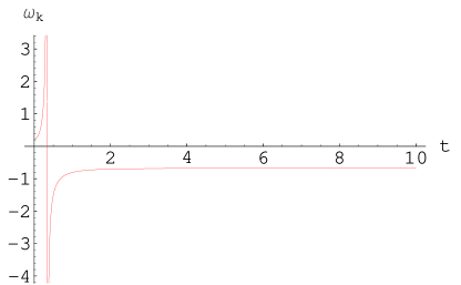
ฯ‰k=โˆ’1+1โˆ’11/3โ€‹t2+6โ€‹tanhโกt+5โ€‹tanh2โกt9โˆ’3/t2+18โ€‹tanhโกt+9โ€‹tanh2โกt.subscript๐œ”๐‘˜11113superscript๐‘ก26๐‘ก5superscript2๐‘ก93superscript๐‘ก218๐‘ก9superscript2๐‘ก\omega_{k}=-1+\frac{1-11/3t^{2}+6\tanh{t}+5\tanh^{2}{t}}{9-3/t^{2}+18\tanh{t}+9\tanh^{2}{t}}. (53)

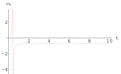
For late time acceleration, i.e., tโ†’โˆžโ†’๐‘กt\rightarrow\infty, this yields

ฯ‰kโˆฃtโ†’โˆž=โˆ’23evaluated-atsubscript๐œ”๐‘˜โ†’๐‘ก23\omega_{k}\mid_{t\rightarrow\infty}=-\frac{2}{3} (54)
Refer to caption
Figure 1: Plot of ฯ‰ksubscript๐œ”๐‘˜\omega_{k} versus cosmic time t๐‘กt for model I.
Refer to caption
Figure 2: Plot of q๐‘žq versus cosmic time t๐‘กt for model I.

which is shown in Figure 1. This represents evolution of k-essence EoS parameter ฯ‰ksubscript๐œ”๐‘˜\omega_{k} as a function of cosmic time. It is obvious that initially (t=0),ฯ‰k=0.22๐‘ก0subscript๐œ”๐‘˜0.22(t=0),~{}\omega_{k}=0.22 showing that the universe is lying in a region which contained dust fluid as well as radiation. As the time elapses up to t=0.42๐‘ก0.42t=0.42, k-essence EoS parameter confined in the region โˆ’โˆž<ฯ‰k<+โˆžsubscript๐œ”๐‘˜-\infty<\omega_{k}<+\infty, i.e., the universe evolutes from physical matter to DE phase. The EoS parameter bears a negative increment in its value and becomes constant at t=0.48๐‘ก0.48t=0.48 towards tโ†’โˆžโ†’๐‘กt\rightarrow\infty. The constant value of EoS parameter is greater than โˆ’11-1 but less than โˆ’1/313-1/3 which shows a quintessence era [21].

The deceleration parameter (25) for this model takes the form

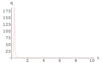
q=โˆ’1+ฮผ1โ€‹(1โˆ’tanh2โกt)ฮผ02+ฮผ12โ€‹tanh2โกt+2โ€‹ฮผ0โ€‹ฮผ1โ€‹tanhโกt๐‘ž1subscript๐œ‡11superscript2๐‘กsuperscriptsubscript๐œ‡02superscriptsubscript๐œ‡12superscript2๐‘ก2subscript๐œ‡0subscript๐œ‡1๐‘กq=-1+\frac{\mu_{1}(1-\tanh^{2}{t})}{\mu_{0}^{2}+\mu_{1}^{2}\tanh^{2}{t}+2\mu_{0}\mu_{1}\tanh{t}} (55)

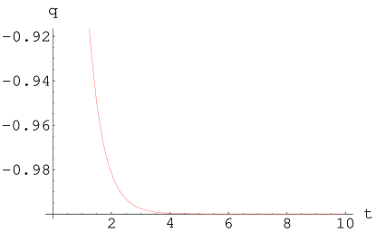
which implies that qโˆฃtโ†’โˆž=โˆ’1evaluated-at๐‘žโ†’๐‘ก1q\mid_{t\rightarrow\infty}=-1 indicating an accelerating universe. Its graphical representation is shown in Figure 2 which indicates that initially at (t=0),q=0๐‘ก0๐‘ž0(t=0),~{}q=0 expressing an expanding universe with a constant velocity. As time passes, its value decreases and converges towards โˆ’11-1. Notice that the graph exhibits an ever expanding universe as there is not a single positive value of q๐‘žq.

4.2 Model II

The second k-essence model [15] is given by

K=โˆ‘j=โˆ’mnฮฝjโ€‹(t)โ€‹ejโ€‹t,๐พsubscriptsuperscript๐‘›๐‘—๐‘šsubscript๐œˆ๐‘—๐‘กsuperscript๐‘’๐‘—๐‘กK=\sum^{n}_{j=-m}\nu_{j}(t)e^{jt}, (56)

where m๐‘šm is any positive real number and nโ‰ค0๐‘›0n\leq 0 real number. For the sake of simplicity, we take m=2,n=0formulae-sequence๐‘š2๐‘›0m=2,~{}n=0 and ฮฝjโ€‹(t)=ฮฝjsubscript๐œˆ๐‘—๐‘กsubscript๐œˆ๐‘—\nu_{j}(t)=\nu_{j} as a constant. Thus

K=ฮฝโˆ’2โ€‹eโˆ’2โ€‹t+ฮฝโˆ’1โ€‹eโˆ’t+ฮฝ0.๐พsubscript๐œˆ2superscript๐‘’2๐‘กsubscript๐œˆ1superscript๐‘’๐‘กsubscript๐œˆ0K=\nu_{-2}e^{-2t}+\nu_{-1}e^{-t}+\nu_{0}. (57)

We also assume H๐ปH as follows

H=ฮผโˆ’1โ€‹eโˆ’t+ฮผ0.๐ปsubscript๐œ‡1superscript๐‘’๐‘กsubscript๐œ‡0H=\mu_{-1}e^{-t}+\mu_{0}. (58)

Inserting this value in Eq.(35), we get

K=9โ€‹ฮผ02+Lโˆ’3โ€‹ฮผโˆ’1โ€‹(1โˆ’6โ€‹ฮผ0)โ€‹eโˆ’t+9โ€‹ฮผโˆ’12โ€‹eโˆ’2โ€‹t.๐พ9superscriptsubscript๐œ‡02๐ฟ3subscript๐œ‡116subscript๐œ‡0superscript๐‘’๐‘ก9superscriptsubscript๐œ‡12superscript๐‘’2๐‘กK=9\mu_{0}^{2}+L-3\mu_{-1}(1-6\mu_{0})e^{-t}+9\mu_{-1}^{2}e^{-2t}. (59)

Using Eqs.(58) and (59) in (34), we obtain kinetic term of k-essence model in the form

X=a2โ€‹eโˆซg2โ€‹(t)โ€‹๐‘‘t.๐‘‹subscript๐‘Ž2superscript๐‘’subscript๐‘”2๐‘กdifferential-d๐‘กX=a_{2}e^{\int g_{2}(t)dt}. (60)

Here a2subscript๐‘Ž2a_{2} is an integration constant and g2โ€‹(t)subscript๐‘”2๐‘กg_{2}(t) is given by

g2โ€‹(t)=2โ€‹[Lห™+3โ€‹ฮผโˆ’1โ€‹(1โˆ’6โ€‹ฮผ0)โ€‹eโˆ’tโˆ’18โ€‹ฮผโˆ’12โ€‹eโˆ’2โ€‹t]3โ€‹J/2โˆ’9/2+Lโˆ’3โ€‹ฮผโˆ’1โ€‹(1+3โ€‹ฮผ0)โ€‹eโˆ’tโˆ’9โ€‹ฮผโˆ’12โ€‹eโˆ’2โ€‹t.subscript๐‘”2๐‘ก2delimited-[]ห™๐ฟ3subscript๐œ‡116subscript๐œ‡0superscript๐‘’๐‘ก18superscriptsubscript๐œ‡12superscript๐‘’2๐‘ก3๐ฝ292๐ฟ3subscript๐œ‡113subscript๐œ‡0superscript๐‘’๐‘ก9superscriptsubscript๐œ‡12superscript๐‘’2๐‘กg_{2}(t)=\frac{2[\dot{L}+3\mu_{-1}(1-6\mu_{0})e^{-t}-18\mu_{-1}^{2}e^{-2t}]}{3J/2-9/2+L-3\mu_{-1}(1+3\mu_{0})e^{-t}-9\mu_{-1}^{2}e^{-2t}}. (61)

The scalar function ฯ•italic-ฯ•\phi is obtained by inserting Eq.(60) in (36).
Refer to caption
Figure 3: Plot of ฯ‰ksubscript๐œ”๐‘˜\omega_{k} versus cosmic time for model II.
Refer to caption
Figure 4: Plot of q๐‘žq versus cosmic time for model II.

The energy density and pressure parameters turn out to be

ฯksubscript๐œŒ๐‘˜\displaystyle\rho_{k} =\displaystyle= โˆ’272โ€‹ฮผ02+32โ€‹Jโˆ’27โ€‹ฮผโˆ’1โ€‹ฮผ0โ€‹eโˆ’tโˆ’272โ€‹ฮผโˆ’12โ€‹eโˆ’2โ€‹t,272superscriptsubscript๐œ‡0232๐ฝ27subscript๐œ‡1subscript๐œ‡0superscript๐‘’๐‘ก272superscriptsubscript๐œ‡12superscript๐‘’2๐‘ก\displaystyle-\frac{27}{2}\mu_{0}^{2}+\frac{3}{2}J-27\mu_{-1}\mu_{0}e^{-t}-\frac{27}{2}\mu_{-1}^{2}e^{-2t}, (62)
pksubscript๐‘๐‘˜\displaystyle p_{k} =\displaystyle= 9โ€‹ฮผ02+Lโˆ’3โ€‹ฮผโˆ’1โ€‹(1โˆ’6โ€‹ฮผ0)โ€‹eโˆ’t+9โ€‹ฮผโˆ’12โ€‹eโˆ’2โ€‹t.9superscriptsubscript๐œ‡02๐ฟ3subscript๐œ‡116subscript๐œ‡0superscript๐‘’๐‘ก9superscriptsubscript๐œ‡12superscript๐‘’2๐‘ก\displaystyle 9\mu_{0}^{2}+L-3\mu_{-1}(1-6\mu_{0})e^{-t}+9\mu_{-1}^{2}e^{-2t}. (63)

Inserting these values in Eq.(43), the EoS parameter takes the form

ฯ‰k=โˆ’1+9โ€‹ฮผ02โˆ’2โ€‹Lโˆ’3โ€‹J+6โ€‹ฮผโˆ’1โ€‹(1+3โ€‹ฮผ0)โ€‹eโˆ’t+9โ€‹ฮผโˆ’12โ€‹eโˆ’2โ€‹t27โ€‹ฮผ02โˆ’3โ€‹J+54โ€‹ฮผโˆ’1โ€‹ฮผ0โ€‹eโˆ’t+27โ€‹ฮผโˆ’1โ€‹eโˆ’2โ€‹t.subscript๐œ”๐‘˜19superscriptsubscript๐œ‡022๐ฟ3๐ฝ6subscript๐œ‡113subscript๐œ‡0superscript๐‘’๐‘ก9superscriptsubscript๐œ‡12superscript๐‘’2๐‘ก27superscriptsubscript๐œ‡023๐ฝ54subscript๐œ‡1subscript๐œ‡0superscript๐‘’๐‘ก27subscript๐œ‡1superscript๐‘’2๐‘ก\omega_{k}=-1+\frac{9\mu_{0}^{2}-2L-3J+6\mu_{-1}(1+3\mu_{0})e^{-t}+9\mu_{-1}^{2}e^{-2t}}{27\mu_{0}^{2}-3J+54\mu_{-1}\mu_{0}e^{-t}+27\mu_{-1}e^{-2t}}. (64)

Taking all the constants equal to 111 as in isotropic case and using Eq.(42), it follows that

ฯ‰k=โˆ’1+9โˆ’11/t2+24โ€‹eโˆ’t+9โ€‹eโˆ’2โ€‹t27โˆ’9/t2+54โ€‹eโˆ’t+27โ€‹eโˆ’2โ€‹t.subscript๐œ”๐‘˜1911superscript๐‘ก224superscript๐‘’๐‘ก9superscript๐‘’2๐‘ก279superscript๐‘ก254superscript๐‘’๐‘ก27superscript๐‘’2๐‘ก\omega_{k}=-1+\frac{9-11/t^{2}+24e^{-t}+9e^{-2t}}{27-9/t^{2}+54e^{-t}+27e^{-2t}}. (65)

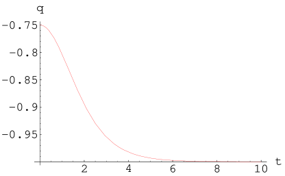
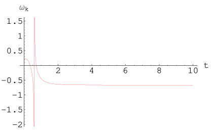
This shows that as tโ†’โˆž,ฯ‰k>โˆ’1formulae-sequenceโ†’๐‘กsubscript๐œ”๐‘˜1t\rightarrow\infty,~{}\omega_{k}>-1 which represents quintessence region [21] shown in Figure 3. This model has the same behavior as that of the first model. However, the EoS parameter is directed to DE era at t=0.34๐‘ก0.34t=0.34 and after a short interval of time, it becomes constant, i.e., โˆ’0.670.67-0.67. The corresponding deceleration parameter is

q=โˆ’1+ฮผโˆ’1โ€‹eโˆ’tฮผโˆ’12โ€‹eโˆ’2โ€‹t+ฮผ02+2โ€‹ฮผโˆ’1โ€‹ฮผ0โ€‹eโˆ’t,๐‘ž1subscript๐œ‡1superscript๐‘’๐‘กsuperscriptsubscript๐œ‡12superscript๐‘’2๐‘กsuperscriptsubscript๐œ‡022subscript๐œ‡1subscript๐œ‡0superscript๐‘’๐‘กq=-1+\frac{\mu_{-1}e^{-t}}{\mu_{-1}^{2}e^{-2t}+\mu_{0}^{2}+2\mu_{-1}\mu_{0}e^{-t}}, (66)

which gives qโˆฃtโ†’โˆž=โˆ’1evaluated-at๐‘žโ†’๐‘ก1q\mid_{t\rightarrow\infty}=-1. At t=0๐‘ก0t=0, the value of q๐‘žq is negative which shows initially an expanding universe. Its value decreases and converges to โˆ’11-1 as tโ†’โˆžโ†’๐‘กt\rightarrow\infty with the passage of time as shown in Figure 4.

4.3 Model III

Here we take the following k-essence model [15]

K=โˆ‘j=โˆ’mnฮฝjโ€‹(t)โ€‹(lnโกt)j,๐พsubscriptsuperscript๐‘›๐‘—๐‘šsubscript๐œˆ๐‘—๐‘กsuperscript๐‘ก๐‘—K=\sum^{n}_{j=-m}\nu_{j}(t)(\ln{t})^{j}, (67)

where m,n๐‘š๐‘›m,~{}n and ฮฝjsubscript๐œˆ๐‘—\nu_{j} are the same as in model II. For m=2,n=0formulae-sequence๐‘š2๐‘›0m=2,~{}n=0 and constant ฮฝjsubscript๐œˆ๐‘—\nu_{j}โ€™s, this equation becomes

K=ฮฝโˆ’2โ€‹(lnโกt)โˆ’2+ฮฝโˆ’1โ€‹(lnโกt)โˆ’1+ฮฝ0.๐พsubscript๐œˆ2superscript๐‘ก2subscript๐œˆ1superscript๐‘ก1subscript๐œˆ0K=\nu_{-2}(\ln{t})^{-2}+\nu_{-1}(\ln{t})^{-1}+\nu_{0}. (68)

Assuming the Hubble parameter in the form

H=ฮผโˆ’1โ€‹(lnโกt)โˆ’1+ฮผ0.๐ปsubscript๐œ‡1superscript๐‘ก1subscript๐œ‡0H=\mu_{-1}(\ln{t})^{-1}+\mu_{0}. (69)

Inserting this value of H๐ปH in Eq.(35), it implies that

K=L+9โ€‹ฮผ02+18โ€‹ฮผโˆ’1โ€‹ฮผ0โ€‹(lnโกt)โˆ’1+3โ€‹ฮผโˆ’1โ€‹(3โ€‹ฮผโˆ’1โˆ’1/t)โ€‹(lnโกt)โˆ’2.๐พ๐ฟ9superscriptsubscript๐œ‡0218subscript๐œ‡1subscript๐œ‡0superscript๐‘ก13subscript๐œ‡13subscript๐œ‡11๐‘กsuperscript๐‘ก2K=L+9\mu_{0}^{2}+18\mu_{-1}\mu_{0}(\ln{t})^{-1}+3\mu_{-1}(3\mu_{-1}-1/t)(\ln{t})^{-2}. (70)

The kinetic term X๐‘‹X from (34) and the corresponding scalar function ฯ•italic-ฯ•\phi become

X=a3โ€‹eโˆซg3โ€‹(t)โ€‹๐‘‘t,ฯ•=โˆ‚tโˆ’1โˆ’2โ€‹X,formulae-sequence๐‘‹subscript๐‘Ž3superscript๐‘’subscript๐‘”3๐‘กdifferential-d๐‘กitalic-ฯ•superscriptsubscript๐‘ก12๐‘‹\displaystyle X=a_{3}e^{\int g_{3}(t)dt},\quad\phi=\partial_{t}^{-1}\sqrt{-2X}, (71)

where g3โ€‹(t)subscript๐‘”3๐‘กg_{3}(t) is found by using (34)

g3โ€‹(t)=2โ€‹[Lห™โˆ’6โ€‹ฮผโˆ’1โ€‹(3โ€‹ฮผโˆ’1โˆ’1/t)โ€‹tโˆ’1โ€‹(lnโกt)โˆ’3+3โ€‹ฮผโˆ’1โ€‹(1/tโˆ’6โ€‹ฮผ0)โ€‹tโˆ’1โ€‹(lnโกt)โˆ’2]subscript๐‘”3๐‘ก2delimited-[]ห™๐ฟ6subscript๐œ‡13subscript๐œ‡11๐‘กsuperscript๐‘ก1superscript๐‘ก33subscript๐œ‡11๐‘ก6subscript๐œ‡0superscript๐‘ก1superscript๐‘ก2\displaystyle g_{3}(t)=2[\dot{L}-6\mu_{-1}(3\mu_{-1}-1/t)t^{-1}(\ln{t})^{-3}+3\mu_{-1}(1/t-6\mu_{0})t^{-1}(\ln{t})^{-2}]
ร—[L+3โ€‹J/2โˆ’9โ€‹ฮผ02/2โˆ’9โ€‹ฮผโˆ’1โ€‹ฮผ0โ€‹(lnโกt)โˆ’1+3โ€‹ฮผโˆ’1โ€‹(โˆ’3โ€‹ฮผโˆ’1/2โˆ’1/t)โ€‹(lnโกt)โˆ’2]โˆ’1.absentsuperscriptdelimited-[]๐ฟ3๐ฝ29superscriptsubscript๐œ‡0229subscript๐œ‡1subscript๐œ‡0superscript๐‘ก13subscript๐œ‡13subscript๐œ‡121๐‘กsuperscript๐‘ก21\displaystyle\times[L+3J/2-9\mu_{0}^{2}/2-9\mu_{-1}\mu_{0}(\ln{t})^{-1}+3\mu_{-1}(-3\mu_{-1}/2-1/t)(\ln{t})^{-2}]^{-1}.
Refer to caption
Figure 5: Plot of ฯ‰ksubscript๐œ”๐‘˜\omega_{k} versus cosmic time for model III.
Refer to caption
Figure 6: Plot of q๐‘žq versus cosmic time for model III.

For this model, ฯksubscript๐œŒ๐‘˜\rho_{k} and pksubscript๐‘๐‘˜p_{k} become

ฯksubscript๐œŒ๐‘˜\displaystyle\rho_{k} =\displaystyle= 32โ€‹Jโˆ’272โ€‹ฮผ02โˆ’27โ€‹ฮผโˆ’1โ€‹ฮผ0โ€‹(lnโกt)โˆ’1โˆ’272โ€‹ฮผโˆ’12โ€‹(lnโกt)โˆ’2,32๐ฝ272superscriptsubscript๐œ‡0227subscript๐œ‡1subscript๐œ‡0superscript๐‘ก1272superscriptsubscript๐œ‡12superscript๐‘ก2\displaystyle\frac{3}{2}J-\frac{27}{2}\mu_{0}^{2}-27\mu_{-1}\mu_{0}(\ln{t})^{-1}-\frac{27}{2}\mu_{-1}^{2}(\ln{t})^{-2}, (73)
pksubscript๐‘๐‘˜\displaystyle p_{k} =\displaystyle= L+9โ€‹ฮผ02+18โ€‹ฮผ0โ€‹ฮผโˆ’1โ€‹(lnโกt)โˆ’1+3โ€‹ฮผโˆ’1โ€‹(3โ€‹ฮผโˆ’1โˆ’1t)โ€‹(lnโกt)โˆ’2.๐ฟ9superscriptsubscript๐œ‡0218subscript๐œ‡0subscript๐œ‡1superscript๐‘ก13subscript๐œ‡13subscript๐œ‡11๐‘กsuperscript๐‘ก2\displaystyle L+9\mu_{0}^{2}+18\mu_{0}\mu_{-1}(\ln{t})^{-1}+3\mu_{-1}(3\mu_{-1}-\frac{1}{t})(\ln{t})^{-2}. (74)

The corresponding EoS parameter takes the form

ฯ‰k=โˆ’1+2โ€‹L+3โ€‹Jโˆ’9โ€‹ฮผ02โˆ’18โ€‹ฮผโˆ’1โ€‹ฮผ0โ€‹(lnโกt)โˆ’1โˆ’6โ€‹ฮผโˆ’1โ€‹(3โ€‹ฮผโˆ’1/2+1/t)โ€‹(lnโกt)โˆ’23โ€‹Jโˆ’27โ€‹ฮผ02โˆ’54โ€‹ฮผโˆ’1โ€‹ฮผ0โ€‹(lnโกt)โˆ’1โˆ’27โ€‹ฮผโˆ’12โ€‹(lnโกt)โˆ’2.subscript๐œ”๐‘˜12๐ฟ3๐ฝ9superscriptsubscript๐œ‡0218subscript๐œ‡1subscript๐œ‡0superscript๐‘ก16subscript๐œ‡13subscript๐œ‡121๐‘กsuperscript๐‘ก23๐ฝ27superscriptsubscript๐œ‡0254subscript๐œ‡1subscript๐œ‡0superscript๐‘ก127superscriptsubscript๐œ‡12superscript๐‘ก2\omega_{k}=-1+\frac{2L+3J-9\mu_{0}^{2}-18\mu_{-1}\mu_{0}(\ln{t})^{-1}-6\mu_{-1}(3\mu_{-1}/2+1/t)(\ln{t})^{-2}}{3J-27\mu_{0}^{2}-54\mu_{-1}\mu_{0}(\ln{t})^{-1}-27\mu_{-1}^{2}(\ln{t})^{-2}}. (75)

To expose the present day nature of the universe, we take ฮผi=mi=si=1subscript๐œ‡๐‘–subscript๐‘š๐‘–subscript๐‘ ๐‘–1\mu_{i}=m_{i}=s_{i}=1 and using Eq.(42), it follows that

ฯ‰k=โˆ’1+3โˆ’11/3โ€‹t2+6โ€‹(lnโกt)โˆ’1+2โ€‹(3/2+1/t)โ€‹(lnโกt)โˆ’29โˆ’3/t2+18โ€‹(lnโกt)โˆ’1+9โ€‹(lnโกt)โˆ’2.subscript๐œ”๐‘˜13113superscript๐‘ก26superscript๐‘ก12321๐‘กsuperscript๐‘ก293superscript๐‘ก218superscript๐‘ก19superscript๐‘ก2\omega_{k}=-1+\frac{3-11/3t^{2}+6(\ln{t})^{-1}+2(3/2+1/t)(\ln{t})^{-2}}{9-3/t^{2}+18(\ln{t})^{-1}+9(\ln{t})^{-2}}. (76)

Consequently, the deceleration parameter become

q=โˆ’1+ฮผโˆ’1tโ€‹(lnโกt)2โ€‹[ฮผโˆ’12โ€‹(lnโกt)โˆ’2+ฮผ02+2โ€‹ฮผ0โ€‹ฮผโˆ’1โ€‹(lnโกt)โˆ’1].๐‘ž1subscript๐œ‡1๐‘กsuperscript๐‘ก2delimited-[]superscriptsubscript๐œ‡12superscript๐‘ก2superscriptsubscript๐œ‡022subscript๐œ‡0subscript๐œ‡1superscript๐‘ก1q=-1+\frac{\mu_{-1}}{t(\ln{t})^{2}[\mu_{-1}^{2}(\ln{t})^{-2}+\mu_{0}^{2}+2\mu_{0}\mu_{-1}(\ln{t})^{-1}]}. (77)

This shows that the condition for accelerating universe is satisfied as tโ†’โˆžโ†’๐‘กt\rightarrow\infty. Figure 5 (76) shows that ฯ‰k>โˆ’1subscript๐œ”๐‘˜1\omega_{k}>-1 as tโ†’โˆžโ†’๐‘กt\rightarrow\infty and initially the model represents a universe having both properties of matter and radiation. After a very short interval, universe is dominated by DE. It is worthwhile to mention here that at t=0.63๐‘ก0.63t=0.63, the universe changed its phase from DE era to a physical matter dominated era. As compared to the DE phase, the universe stayed in matter dominated era for a short interval of time. Then a decrement in its value is observed, the EoS parameter for k-essence attains negative values and finally converges to a constant value resulting quintessence region [22] of the universe. Figure 6 (77) represents a decelerating universe at early times as the value of q๐‘žq is positively increasing or decreasing at that stage. After a long interval of time, the universe intersects the boundary from matter to DE era and takes q=โˆ’1๐‘ž1q=-1. This corresponds to an accelerating expanding universe.

5 Summary

This paper is devoted to study the well-known phenomenon of the universe expansion in the context of Fโ€‹(T)๐น๐‘‡F(T) gravity. For this purpose, we have taken Bianchi type I๐ผI universe and have explored some purely kinetic k-essence models. In physical cosmology and gravity, the DE problem has been investigated in terms of cosmological constant, scalar fields, tachyon, Chaplygin gas, quintessence and modified gravities etc. Here have used Fโ€‹(T)๐น๐‘‡F(T) gravity and scalar field term whose combination has resulted a quintessence phase.

We have evaluated the EoS parameter and the deceleration parameter for purely kinetic k-essence models. These are shown in terms of graphs versus cosmic time by taking particular values of the metric coefficients. These models describe evolution of the universe from big-bang to present epoch and are summarized as follows

  • โ€ข

    For model I, the EoS parameter and the deceleration parameter indicate an ever accelerating universe with the passage of time. At t=0.42๐‘ก0.42t=0.42, the universe changes its phase from matter dominated to DE phase resulting quintessence region.

  • โ€ข

    The model II has the same behavior as that of the model I, however, phase changes at point t=0.38๐‘ก0.38t=0.38. The deceleration parameter initially represents an expanding universe with constant speed and after a short interval, it accelerates with a faster speed.

  • โ€ข

    For model III, ฯ‰ksubscript๐œ”๐‘˜\omega_{k} and q๐‘žq initially show decelerating DE dominated universe which reverses to matter dominated decelerating universe at t=0.64๐‘ก0.64t=0.64. After a slight increment in time, the universe shows accelerating recent epoch of DE issue lying in the quintessence region.

The analysis of models reveal that the present day universe is dominated by DE component which can successfully describe accelerating nature of the universe consistent with the observations [23]. These new forms of models may give the equivalent descriptions of DE to discuss the acceleration of the expanding universe. These models indicate that the present day universe is dominated by DE component. The viability of these models depend on the possible values of parameters. Similarly, we can construct the observational parameters for other new k-essence models induced by modified gravity theory. Finally, it is worthwhile to mention here that all the above results turn out to be the generalization of the already obtained results for the FRW metric [16]. The graphs of models depend upon the values of parameters accordingly. For Bianchi type I๐ผI, the k-essence models in the context of generalized teleparallel gravity mark out a quintessence DE phase.

References

  • [1] Spergel, D.N. et al.: Astrophys. J. Suppl. 148(2003)175.
  • [2] Hinshaw, G. et al.: Astrophys. J. Suppl. 180(2009)225.
  • [3] de Araujo, J.C.N.: Astropart. Phys. 23(2005)279.
  • [4] Mukhanov, V., Armendariz-Picon, C. and Steinhardt, P.J.: Phys. Rev. Lett. 85(2010)4438.
  • [5] de Putter, R. and Linder, E.V.: Astropart. Phys. 28(2007)263.
  • [6] Armendariz-Picon, C., Damour, T., and Mukhanov, V.: Phys. Lett. B458(1999)209.
  • [7] Nojiri, S.: Towards the Unification of Late-time Acceleration and Inflation by K-essence Model, arXiv/1006.5201v1.
  • [8] Matsumoto, J. and Nojiri, S.: Phys. Lett. B687(2010)236.
  • [9] Armendariz-Picon, C., Mukhanov, V. and Steinhardt, P.J.: Phys. Rev. D63(2001)103510.
  • [10] Bose, N. and Majumdar, A.S.: Phys. Rev. D79(2009)103517.
  • [11] Yang, R.J. and Gao, X.T.: Chin. Phys. Lett. 28(2011)109502.
  • [12] Nojiri, S. et al.: Reconstruction and Deceleration-acceleration Transition in Modified Gravity, arXiv/0912.2488v3.
  • [13] Linder, E.V.: Phys. Rev. D81(2010)127301.
  • [14] Sharif, M. and Amir, M.J.: Mod. Phys. Lett. A22(2007)425; Sharif, M. and Amir, M.J.: Gen. Relativ. Grav. 39(2007)989; Sharif, M. and Amir, M.J.: Int. J. Theor. Phys. 47(2008)1742; Sharif, M.: Braz. J. Phys. 37(2007)1292; Sharif, M. and Nazir, K.: Commun. Theor. Phys. 50(2008)664; Sharif, M. and Taj, S. : Astrophys. Space Sci. 325(2010)75.
  • [15] Myrzakulov, R.: Fโ€‹(T)๐น๐‘‡F(T) Gravity and K-essence, arXiv/1008.4468v2.
  • [16] Tsyba, P.Y. et al.: Int. J. Theor. Phys. 50(2011)1876.
  • [17] Dent, J.B., Dutta, S. and Saridakis, E.N.: JCAP 1101(2011)009.
  • [18] Karami, K. and Abdolmaleki, A.: Original and Entropy-Corrected Versions of the Holographic and New Agegraphic f(T)-Gravity Models, arXiv/1009.2459v1.
  • [19] Vakili, B. and Sepangi, H.R.: JCAP 0509(2005)008.
  • [20] Radinschi, I.: Acta Phys. Slov. 50(2000)609.
  • [21] Steinhardt, P.J.: Phil. Trans. R. Soc. Land. A 361(2003)2497.
  • [22] Riazuelo, A.: Frontiers of Cosmology (Springer, 2005).
  • [23] Carroll, S.M.: Phys. Rev. Lett. 81(1998)3067.