Effective Confinement as Origin of the Equivalence of Kinetic Temperature and Fluctuation-Dissipation Ratio in a Dense Shear Driven Suspension

Abstract

We study response and velocity autocorrelation functions for a tagged particle in a shear driven suspension governed by underdamped stochastic dynamics. We follow the idea of an effective confinement in dense suspensions and exploit a time-scale separation between particle reorganization and vibrational motion. This allows us to approximately derive the fluctuation-dissipation theorem in a “hybrid” form involving the kinetic temperature as an effective temperature and an additive correction term. We show numerically that even in a moderately dense suspension the latter is negligible. We discuss similarities and differences with a simple toy model, a single trapped particle in shear flow.

I Introduction

Equilibrium statistical mechanics describes the connection of a few macroscopic intensive quantities, e.g. pressure and temperature, with the microscopic properties of the many particles constituting the system McQuarrie (2000). Although there is no equivalent formalism for systems driven out of thermal equilibrium studies are often motivated by the quest for simple governing principles such as an effective temperature Cugliandolo et al. (1997); Cugliandolo (2011). Of particular interest are small mesoscopic systems such as colloidal particles, nanoparticles in solution, or biological systems, all of which are dominated by fluctuations.

For systems only slightly perturbed from equilibrium – into what is called the linear response regime – the fluctuation-dissipation theorem (FDT) relates the response with equilibrium correlations through the temperature Kubo et al. (1991). This unique temperature corresponds to what we would measure with a thermometer, and is independent of the observables entering the fluctuation-dissipation theorem. Examples for these observables are the velocity related to the diffusion coefficient, or stress fluctuations determining the viscosity. The practical importance of the FDT both for experiments and simulations thus stems from the possibility to extract transport properties from stationary fluctuations. In a more recent application the FDT has been used to predict the self-assembly of model systems Jack et al. (2007); Klotsa and Jack (2011).

Even for systems driven into a non-equilibrium steady state (NESS) far beyond the linear response regime we can still define a linear response function Agarwal (1972); Hänggi and Thomas (1982); Crisanti and Ritort (2003); Marconi et al. (2008). For the broad class of driven systems with Markovian dynamics and embedded in a fluid at well defined temperature it has been demonstrated recently that then the FDT is most convincingly interpreted in terms of an excess correlation Speck and Seifert (2006); Blickle et al. (2007); Speck and Seifert (2009); Baiesi et al. (2009); Prost et al. (2009); Seifert and Speck (2010); Speck (2010). The single temperature that enters these generalized FDTs is that of the fluid, and no approximations are involved. Nevertheless, for the purpose of a simple description we might still be interested in defining an approximate temperature through the fluctuation-dissipation ratio (FDR), i.e., the ratio of correlation to response function. This strategy has originally been proposed in the context of aging mean-field spin systems Cugliandolo et al. (1997); Cugliandolo (2011), and subsequently been applied to many different systems Ono et al. (2002); Hayashi and Sasa (2004); Haxton and Liu (2007). In particular, in a sheared colloidal suspension or fluid the Einstein relation between the self-diffusion coefficient of a tagged particle and its mobility is broken and can be used to define an effective temperature Berthier and Barrat (2002); Szamel (2004); Krüger and Fuchs (2009); Lander et al. (2010); Zhang and Szamel (2011).

Figure 1: (Color online) Systems studied: (A) Toy model with a single particle bound to the origin and (B) tagged particle in a dense suspension. Both systems are driven through linear shear flow.

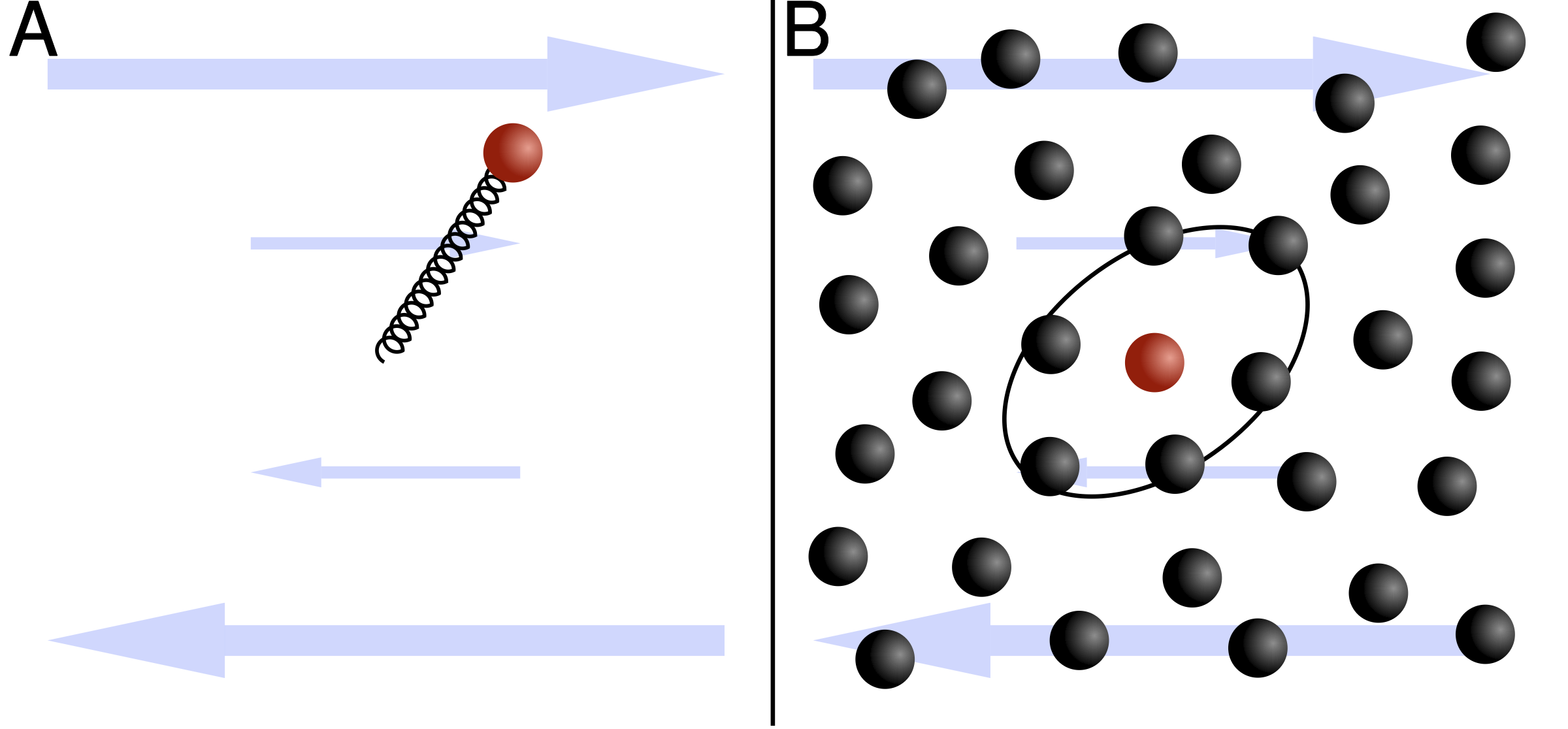
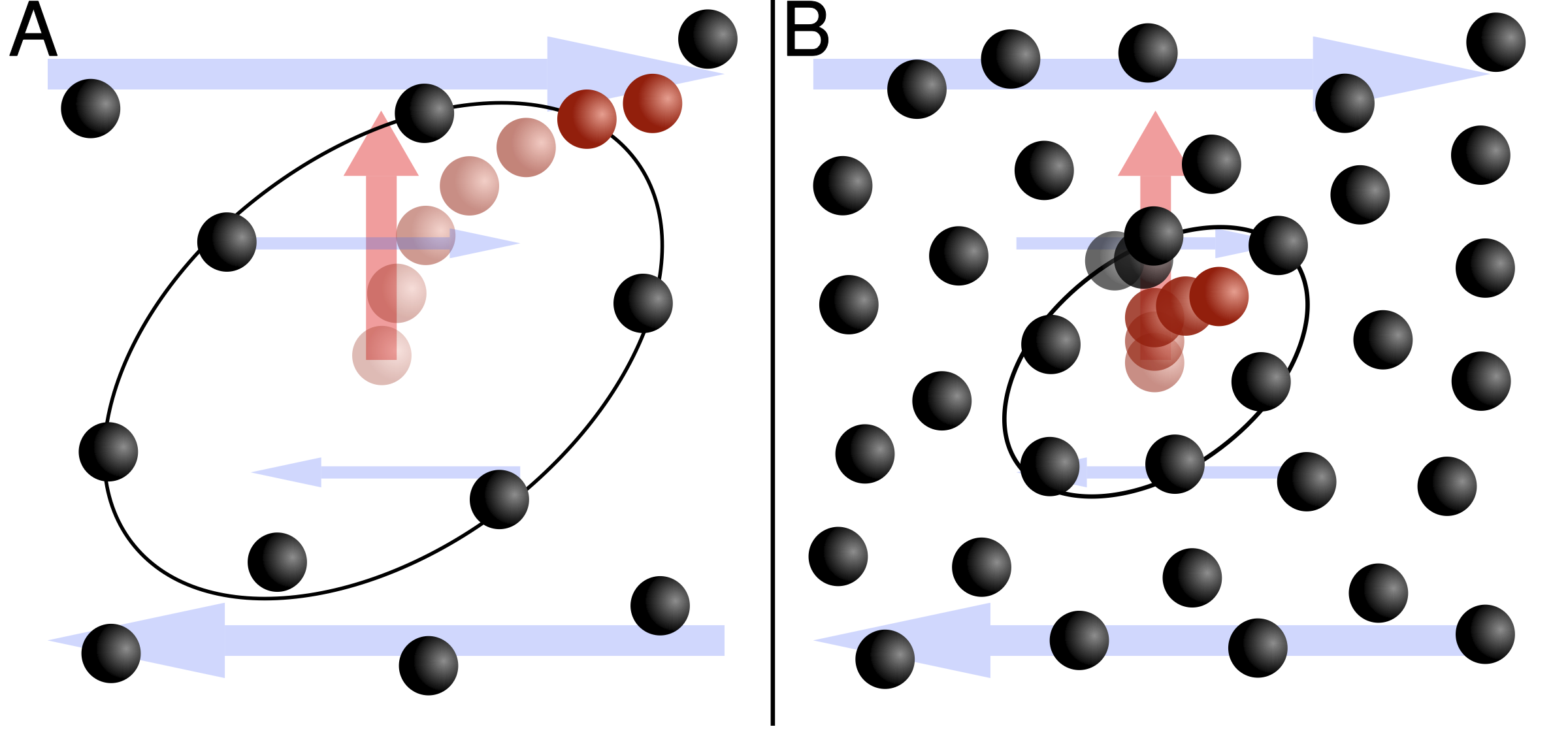
In this paper we study a many-body system governed by underdamped stochastic dynamics and driven into a NESS through linear shear flow. Such a system could model a fluid with every particle coupled to a stochastic thermostat, colloidal or nano-suspensions, or dusty plasmas Shukla (2001). We follow a tagged particle, i.e., a randomly chosen particle out of many identical interacting particles. Motivated by the physical picture of an effective confinement in dense systems we also consider a single trapped colloidal particle in shear flow Ziehl et al. (2009) as a toy model, see Fig. 1. We discuss the FDT in a “hybrid” form: we relate response and correlations through the kinetic temperature in the spirit of an effective temperature, but with an additive correction term still present. For the trapped particle expressions can be obtained analytically. For the tagged particle we derive a similar FDT exploiting a time-scale separation due to the effective confinement. In both cases we show that the correction term indeed becomes negligible for strong confinement.

II Fluctuation-dissipation ratio

We study the response of a single particle with mass $M$ moving in a viscous liquid at temperature $T$. After applying a small external force $\mathbf{f}$ directly to the particle its mean velocity evolves as

$$\langle\mathbf{v}(t)\rangle=\int_{0}^{t}\mathrm{d}t^{\prime}\;\mathsf{R}(t-t^{\prime})\mathbf{f}(t^{\prime})+\mathcal{O}(f^{2}),$$ (1)

where $\mathsf{R}=(R_{ij})$ is the response matrix with components

$$R_{ij}(t-t^{\prime})\equiv\left.\frac{\delta\langle v_{i}(t)\rangle}{\delta f_{j}(t^{\prime})}\right|_{\mathbf{f}=0}$$ (2)

with $t\geqslant t^{\prime}$ due to causality. The brackets $\langle\cdots\rangle$ denote the thermal average in the perturbed system. Throughout this paper we employ dimensionless units and measure length in units of the particle diameter $a$ and energy in units of $k_{\text{B}}T$. Time is measured in units of $\tau_{0}\equiv a^{2}/D_{0}$, which quantifies the time it takes for a free particle with diffusion coefficient $D_{0}$ to diffuse a distance equal to its diameter. The reduced mass $m\equiv(MD_{0}/k_{\text{B}}T)/\tau_{0}$ is the ratio of the momentum relaxation time to the diffusive time scale $\tau_{0}$.

We describe the stochastic particle motion through the coupled equations $\dot{\mathbf{r}}=\mathbf{v}$ and

$$m\dot{\mathbf{v}}=-\nabla U+\mathbf{f}-[\mathbf{v}-\mathbf{u}(\mathbf{r})]+\boldsymbol{\xi},$$ (3)

where $\mathbf{r}$ and $\mathbf{v}$ are the particle position and velocity, respectively. Besides the conservative forces arising from the potential $U$ we can perturb the particle by a direct force $\mathbf{f}$. The noise $\boldsymbol{\xi}$ modeling the interactions of the particle with solvent molecules has zero mean and correlations

$$\langle\boldsymbol{\xi}(t)\boldsymbol{\xi}^{\text{T}}(t^{\prime})\rangle=2\;\mathbf{1}\delta(t-t^{\prime}).$$ (4)

The external shear flow enters through the term $\mathbf{u}(\mathbf{r})=\dot{\gamma}y\mathbf{e}_{x}$, i.e., the flow points in $x$-direction and increases its amplitude linearly with the $y$-coordinate. Here, $\dot{\gamma}$ is the strain rate which in our units is equal to the Péclet number.

Eq. (2) measures the linear response of the system. If the unperturbed system ($\mathbf{f}=0$) is in thermal equilibrium the FDT

$$\mathsf{R}(t-t^{\prime})=\mathsf{C}(t-t^{\prime})\equiv\langle\mathbf{v}(t)\mathbf{v}^{\text{T}}(t^{\prime})\rangle_{0}$$ (5)

relates this response to the velocity auto correlation function (VACF) $\mathsf{C}(t)$, where the subscript indicates that these correlations are to be measured in the unperturbed system.

For a computationally convenient representation of the response function Eq. (2) valid both in and out of equilibrium consider the path weight of the noise

$$P[\boldsymbol{\xi}(t)]\sim\exp\left\{-\frac{1}{4}\int\mathrm{d}t\;[\boldsymbol{\xi}(t)]^{2}\right\}.$$ (6)

The stochastic velocity of the particle is a result of previous collisions with solvent molecules, $\mathbf{v}(t)=\mathbf{v}[t;\boldsymbol{\xi}(\tau)]$. Since a force perturbation is equivalent to perturbing the noise we can write

$$R_{ij}(t-t^{\prime})=\int[\boldsymbol{\xi}(\tau)]\frac{\delta v_{i}[t;\boldsymbol{\xi}(\tau)]}{\delta\xi_{j}(t^{\prime})}P[\boldsymbol{\xi}(\tau)]$$ (7)

for the response. A functional integration by parts then leads to Speck and Seifert (2006); Calabrese and Gambassi (2005)

$$\mathsf{R}(t-t^{\prime})=\frac{1}{2}\langle\mathbf{v}(t)\boldsymbol{\xi}^{\text{T}}(t^{\prime})\rangle_{0}.$$ (8)

Hence, even if the system is driven into a NESS the response can be measured through a steady-state correlation function (see also Refs. Chatelain (2004); Berthier (2007)). However, the FDT in the form Eq. (5) no longer holds and the dimensionless fluctuation-dissipation ratio (FDR) is defined as

$$X_{i}(t)\equiv\frac{C_{ii}(t)}{R_{ii}(t)}$$ (9)

for the diagonal components.

To calculate $X_{i}(0)$ we perform a short-time expansion of Eq. (1) leading to $\langle\mathbf{v}\rangle\approx\Delta t\mathsf{R}(0)\mathbf{f}$. From the equation of motion (3) we obtain $m\langle\dot{\mathbf{v}}\rangle_{0}\approx m\langle\mathbf{v}\rangle/\Delta t=\mathbf{f}$. We have exploited that the average force on the particle right before the perturbation vanishes, $\langle\mathbf{\nabla}U\rangle_{0}=0$, which is quite obvious for isotropic systems but due to the inversion symmetry about the origin it holds also in the presence of simple shear flow. Hence, in our dimensionless units we obtain $R_{ij}(0)=\delta_{ij}/m$ and finally

$$X_{i}(0)=m\langle v_{i}^{2}\rangle_{0}\equiv\theta_{i}.$$ (10)

The right hand side is the kinetic temperature as measured through the velocity fluctuations. In the following we study for two systems whether, and under which conditions, Eq. (10) extends to times $t>0$, i.e., whether $X_{i}(t)\approx\theta_{i}$.

III Trapped particle

The toy model we investigate first is a single particle trapped in the harmonic potential

$$U(r)=\frac{1}{2}kr^{2}$$ (11)

with strength $k$, where $\mathbf{r}$ is the displacement from the origin and $r=|\mathbf{r}|$. Due to the linearity of the restoring force the $z$-component in Eq. (3) decouples and remains in equilibrium, $X_{z}(t)=\theta_{z}=1$. Therefore, in this section we only consider the motion in the $xy$-plane.

III.1 Analytical results

Due to the quadratic potential Eq. (11) the equations of motion comprise a linear system of first order differential equations. Hence, we can solve it for the velocity

$$\mathbf{v}(t)=\mathsf{G}^{vr}(t)\mathbf{r}_{0}+\mathsf{G}^{vv}(t)\mathbf{v}_{0}+\frac{1}{m}\int_{0}^{t}\mathrm{d}t^{\prime}\;\mathsf{G}^{vv}(t-t^{\prime})\boldsymbol{\xi}(t^{\prime})$$ (12)

given the initial displacement $\mathbf{r}_{0}$ and initial velocity $\mathbf{v}_{0}$. The explicit expressions for the Green’s functions $\mathsf{G}(t)$ are given in the appendix A. Both the VACF and the response function are easily calculated from the solution Eq. (12). For the VACF we find

$$\mathsf{C}(t)=\langle\mathbf{v}(t)\mathbf{v}_{0}^{\text{T}}\rangle_{0}=\mathsf{G}^{vr}(t)\langle\mathbf{r}_{0}\mathbf{v}_{0}^{\text{T}}\rangle_{0}+\mathsf{G}^{vv}(t)\langle\mathbf{v}_{0}\mathbf{v}_{0}^{\text{T}}\rangle_{0},$$ (13)

while the response function is trivially related to the Green’s function through

$$\mathsf{R}(t-t^{\prime})=\frac{1}{2}\langle\mathbf{v}(t)\boldsymbol{\xi}^{\text{T}}(t^{\prime})\rangle_{0}=\frac{1}{m}\mathsf{G}^{vv}(t-t^{\prime})$$ (14)

using the noise correlations Eq. (4). From the steady state distribution Eq. (34) we obtain the moments

$$\langle\mathbf{r}_{0}\mathbf{v}_{0}^{\text{T}}\rangle_{0}=\frac{1}{2k}\left(\begin{array}[]{cc}0&-\dot{\gamma}\\ \dot{\gamma}&0\end{array}\right),$$ (17)

$$\langle\mathbf{v}_{0}\mathbf{v}_{0}^{\text{T}}\rangle_{0}=\frac{1}{m}\mathbf{1}+\frac{1}{2k}\left(\begin{array}[]{cc}\dot{\gamma}^{2}&0\\ 0&0\end{array}\right).$$ (20)

The kinetic temperatures Eq. (10) perpendicular to the shear flow are $\theta_{y}=\theta_{z}=1$, whereas

$$\theta_{x}=1+\alpha_{x}\dot{\gamma}^{2}\geqslant 1,\qquad\alpha_{x}\equiv\frac{m}{2k}.$$ (21)

As a consequence of the linear forces and the symmetry of the shear flow the excess compared to equilibrium is proportional to $\dot{\gamma}^{2}$.

Figure 2: (Color online) Single particle moving in a harmonic trap: (A-C) scaled velocity auto-correlation function $C_{xx}(t)/\theta_{x}$ and response function $R_{xx}(t)$ vs. time $t$ for strain rate $\dot{\gamma}=2$ and different masses $m$ and trap strengths $k$. (B,C) For large $k$, the correction in Eq. (22) becomes negligible and both curves lie on top of each other. (D) The magnitude of the correction term $\beta_{x}$ as a function of $k$ for two different masses. (E) Sketch of the different regimes of the FDT for $m=0.6$. The dashed lines $\dot{\gamma}^{2}$ and $1/m$ limit the region where the FDR is approximatly time-independent, $X_{x}\approx\theta_{x}$. Below the solid line $m\dot{\gamma}^{2}$ the kinetic temperature is much larger than unity. While for the chosen $m$ there is a gap (shaded area), with increasing $m$ both regimes can be realized in the vicinity of the solid line.

III.2 The FDT

Using the explicit expressions for the moments we see that with $G^{vr}_{yx}(t)=0$ the correlation function for the $y$-component reads $C_{yy}(t)=G^{vv}_{xx}\langle v_{y}^{2}\rangle_{0}$ and therefore $X_{y}(t)=\theta_{y}=1$ at all times. On the other hand, in the direction of the shear flow we obtain

$$C_{xx}(t)=\theta_{x}R_{xx}(t)+\langle yv_{x}\rangle_{0}G^{vr}_{xy}(t),$$ (22)

i.e., the velocity correlations are expressed through the response times the kinetic temperature plus a correction term. Separating the dependence on strain rate the correction term can be rewritten as

$$\langle yv_{x}\rangle_{0}G^{vr}_{xy}(t)=\dot{\gamma}^{2}\beta_{x}I_{x}(t),$$ (23)

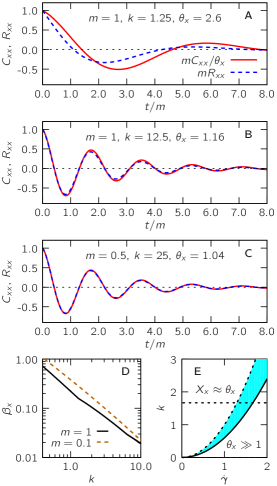
where $\max|I_{x}(t)|=1$ and $\beta_{x}$ captures the magnitude of the correction term. In Fig. 2, we plot scaled response and correlation functions for three representative values of the parameters $m$ and $k$. As demonstrated in Fig. 2D increasing the trap strength $k$ strongly decreases $\beta_{x}$. The behavior of the FDT is sketched in Fig. 2E, where we compare the magnitude of the correction term to the kinetic temperature. From Eq. (21) we see that for $k\ll m\dot{\gamma}^{2}$ we have $\theta_{x}\gg 1$ (see also Fig. 2A). For the relevant case $k\gtrsim 1/m$ we find from the explicit expressions that for the FDR to become approximately time-independent $k\gg\max\{\dot{\gamma}^{2},m\dot{\gamma}^{2}\}$ must hold (Fig. 2C). While for small masses $m<1$ there is a gap (this case is sketched in Fig. 2E), for sufficiently large $m\gtrsim 1$ these two regimes come close. In Fig. 2B, we demonstrate that there is indeed a regime of intermediate trap strength $k\sim m\dot{\gamma}^{2}$ with an increased effective temperature where nevertheless $X_{x}(t)\approx\theta_{x}$ holds to a very good degree.

IV Tagged particle in a suspension

The main system we now study is a suspension composed of $N$ particles in which we tag and follow a single particle, say $k=1$, with position $\mathbf{r}_{1}$ and velocity $\mathbf{v}_{1}$. The particles interact through a pair potential $u(r)$ with total potential energy $U=\sum_{i<j}u(|\mathbf{r}_{i}-\mathbf{r}_{j}|)$. Advection through the shear flow leads to the well-known Taylor dispersion Taylor (1953). Instead of the absolute velocity $\mathbf{v}_{1}$ it will be more convenient to use the relative velocity

$$\mathbf{v}\equiv\mathbf{v}_{1}-\mathbf{u}(\mathbf{r}_{1})$$ (24)

with respect to the flow as the observable entering the response $\mathsf{R}(t)$ and correlation function $\mathsf{C}(t)$.

Figure 3: (Color online) Tagged particle with $m=1$ in a sheared suspension at volume fractions $\phi=0.1$ (top row) and $\phi=0.4$ (bottom row): (A) Pair distribution function in the $xy$-plane for strain rate $\dot{\gamma}=1$. (B) Scaled velocity auto-correlation functions $C_{xx}(t)/\theta_{x}$ and response functions $R_{xx}(t)$ for different strain rates: from bottom to top $\dot{\gamma}=0,0.2,0.4,0.6,0.8,1$. For visibility curves are shifted. (C) Off-diagonal response functions $R_{xy}(t)$ (solid lines) and $R_{yx}(t)$ (dashed lines) for the same strain rates and offsets. (D) The magnitude of the correction term $|\theta_{xy}R^{\ast}_{ij}|$, i.e., the product of Eq. (29) with the maximum $R^{\ast}_{ij}$ of the off-diagonal response function, as a function of strain rate. The dashed lines show the quadratic fits.

IV.1 Time-scale separation

In the following we assume a time scale separation between the motion of the potential energy minimum (or inherent state position Stillinger and Weber (1984)) $\mathbf{r}_{\text{c}}$, and the vibrational motion of the tagged particle around $\mathbf{r}_{\text{c}}$. The physical picture is that particles vibrate in a “cage” of surrounding particles and that local reorganization takes much longer than the vibrational motion. Linearizing the force exerted by neighboring particles on the tagged particle leads to

$$-\nabla_{1}U\approx-\mathsf{k}[\mathbf{r}_{1}(t)-\mathbf{r}_{\text{c}}(t)],\qquad k_{ij}\equiv\left.\frac{\partial^{2}U}{\partial r_{i}\partial r_{j}}\right|_{\mathbf{r}=\mathbf{r}_{\text{c}}}.$$ (25)

We solve the resulting equations of motion leading to the same formal result Eq. (13) for the correlation function and Eq. (14) the response function. In principle the Green’s function can be calculated but we will not need its explicit form here. To see that the first term in Eq. (13) vanishes consider the projected probability

$$\bar{\psi}_{\text{s}}(\mathbf{r}_{1},\mathbf{v})=\int\mathrm{d}\mathbf{r}_{2}\cdots\mathrm{d}\mathbf{r}_{N}\;\int\mathrm{d}\mathbf{v}_{2}\cdots\mathrm{d}\mathbf{v}_{N}\;\psi_{\text{s}}(\{\mathbf{r}_{i}\})$$ (26)

of the tagged particle, where $\psi_{\text{s}}$ is the full stationary distribution. For a homogeneous, translationally invariant system $\bar{\psi}_{\text{s}}$ cannot depend on the position $\mathbf{r}_{1}$ and therefore $\langle\mathbf{r}_{1}\mathbf{v}^{\text{T}}\rangle_{0}\sim\langle\mathbf{v}\rangle_{0}=0$ vanishes. Hence, we obtain

$$C_{ii}(t)=\theta_{i}R_{ii}(t)+m\sum_{j\neq i}\langle v_{i}v_{j}\rangle_{0}R_{ij}(t)$$ (27)

as our central result. The correction term differs from Eq. (22) and now couples to the off-diagonal elements of the response function instead of the off-diagonal component of the Green’s function connecting velocity and position.

IV.2 Langevin dynamics simulations

We perform Langevin dynamics simulations to study Eq. (27) for a specific system. The $N=1728$ particles are enclosed in a cubic simulation box with edge length $L$. The particles interact through the Yukawa (or screened Coulomb) pair potential

$$u(r)=\begin{cases}\varepsilon\frac{e^{-\kappa(r-1)}}{r}&(r\geqslant 1)\\ \infty&(r<1),\end{cases}$$ (28)

where $\varepsilon$ is the interaction energy at contact and $\kappa^{-1}$ the screening length determined by the composition of the surrounding solvent. We choose $\varepsilon=8.0$ and $\kappa=5.0$ in order to obtain a broad range of densities for which the liquid phase is stable Azhar et al. (2000). For the shear flow we employ Lees-Edwards boundary conditions, which enforce a linear velocity profile in the suspension Allen and Tildesley (1987). We integrate the equations of motion by a stochastic velocity Verlet algorithm Frenkel and Smit (2002) with a time step $5\times 10^{-4}$. Since the hard-core repulsion cannot be implemented in the interaction potential we employ a simple algorithm that detects collisions and computes the appropriate positions and velocities after the impact according to momentum and energy conservation (see Refs. Strating (1999); Foss and Brady (2000) and references therein). The NESSs are prepared by initializing the particle positions on a regular lattice at low density. Then we equilibrate the system and slowly increase the density by decreasing the box size. After this equilibrium system is constructed we slowly ramp up the strain rate until the target value $\dot{\gamma}$ is reached. We simulate another $1000$ time steps to relax the system into the steady state. This procedure is repeated separately for independent runs.

We study suspensions at different volume fractions $\phi\equiv\pi N/(6L^{3})$ and strain rates $\dot{\gamma}$. To determine the response and correlation functions we simulate the motion of the system in the NESS and record the velocity trajectories of $200$ randomly chosen particles in four independent runs. From this data we can easily evaluate the VACF. To compute the response to a small force we again employ Eq. (8), which is still valid for the many particle system. This enables us to obtain the response function from steady state trajectories without the need to explicitly perturb the system. Therefore, in addition to the velocity, we also record the stochastic forces acting on the tagged particles, which are directly accessible in a numerical simulation.

IV.3 Numerical results

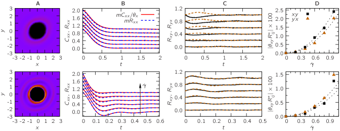
The pair distribution function quantifies the probability to find another particle at a displacement $\mathbf{r}$. It is distorted from its isotropic equilibrium shape, see Fig. 3A. This function visualizes the average environment of the tagged particle. Under the influence of the shear flow there is a higher number of particles in the compressional zones and a depletion in the extensional zones Foss and Brady (2000). Moreover, the peak corresponding to the first nearest-neighbor shell becomes more pronounced.

Figure 4: (Color online) Dilute suspension at $\phi=0.01$ and strain rate $\dot{\gamma}=1$ (left) and $\dot{\gamma}=2$ (right). In comparison to Fig. 3 a deviation between response $R_{xx}(t)$ and velocity autocorrelation function $C_{xx}(t)$ is observed.

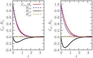
In Fig. 3B, the response functions $R_{xx}(t)$ together with the scaled VACF $C_{xx}(t)/\theta_{x}$ is plotted for volume fractions $\phi=0.1$ and $\phi=0.4$, and for a range of strain rates. Even for times $t>0$ these functions coincide, which implies that the additive correction term in Eq. (27) vanishes. The off-diagonal response functions are plotted in Fig. 3C. For comparison response and correlation functions are plotted in Fig. 4 for a dilute suspension at volume fraction $\phi=0.01$. Here we observe a clear difference between correlations and response. To understand the observed behavior one should bear in mind that we consider the velocities relative to the local flow. At low densities collisions are rare and the particles adapt smoothly to the flow of the solvent. Therefore, the largest deviations from the flow profile arise when a particle diffuses in $y$-direction entering a region of faster or slower flow in $x$-direction, to which it needs to adapt. For higher densities collisions become much more frequent. These collisions prevent the particles from adapting to the solvent flow. Additionally they distribute the momentum, transfered to the particles by the shear flow, more or less randomly in the three spacial directions. The result is that under shear flow the diagonal velocity moments grow with increasing density, and become more and more similar in size.

The two components $\langle v_{x}v_{z}\rangle_{0}\simeq 0$ and $\langle v_{y}v_{z}\rangle_{0}\simeq 0$ of the velocity correlation matrix are very small (see also Fig. 7). Defining the off-diagonal “temperature”

$$\theta_{xy}\equiv m\langle v_{x}v_{y}\rangle_{0}$$ (29)

we see that the dominant contribution to the correction term in Eq. (27) is $\theta_{xy}R_{xy}(t)$ for the $x$ component, and $\theta_{xy}R_{yx}(t)$ for the $y$ component. In analogy to the trapped particle [Eq. (23)] we separate the strain rate dependence of the correction terms,

$$\theta_{xy}R_{xy}(t)\approx\dot{\gamma}^{2}\beta_{x}I_{x}(t),\quad\theta_{xy}R_{yx}(t)\approx\dot{\gamma}^{2}\beta_{y}I_{y}(t),$$ (30)

with again $\max|I_{i}(t)|=1$ and coefficients $\beta_{i}$. In Fig. 3D, we plot $|\theta_{xy}R^{\ast}_{ij}|\approx\dot{\gamma}^{2}\beta_{i}$, where $R^{\ast}_{ij}$ is the maximal value of the off-diagonal component of the response matrix. For $\phi=0.1$ we observe the predicted quadratic dependence on the strain rate $\dot{\gamma}$. For $\phi=0.4$ the quadratic predicition holds for $\dot{\gamma}\leqslant 0.8$, while for larger strain rates higher order terms in $\dot{\gamma}$ become important.

Figure 5: (Color online) The kinetic temperatures $\theta_{i}$ (symbols) and their quadratic fits (lines) plotted vs. strain rate $\dot{\gamma}$ for $m=1$. Shown are the three directions for volume fractions (A) $\phi=0.1$ and (B) $\phi=0.4$. In (C) the coefficients $\alpha_{i}$ and $\beta_{x}\times 10^{2}$ are plotted as function of the volume fraction $\phi$. (D) Relative magnitude of the correction term $|\theta_{xy}R^{\ast}_{xy}|/\theta_{x}\times 10^{3}$ as function of strain rate and density, cf. Fig. 2E. Colors are linearly interpolated.

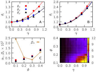
In Fig. 5, we plot the kinetic temperatures as a function of strain rate. While for $\phi=0.1$ a clear difference between motion parallel to the flow ($\theta_{x}$) and motion perpendicular to the flow ($\theta_{y}\simeq\theta_{z}$) can be seen, this distinction is diminished at higher densities. Moreover, all kinetic temperatures can be well fitted by the quadratic function Eq. (21) with coefficients $\alpha_{i}$ for the three directions. The increase of velocity fluctuations can be explained by forced collisions due to the flow gradient, an effect that is more pronouned at higher densities and higher strain rates.

In Fig. 5C, the coefficients $\alpha_{i}$ and $\beta_{x}$ are shown for the different densities. The coefficient $\beta_{x}$ decreases for larger densities but then turns up again at $\phi=0.4$. The reason for this non-monotonic behavior is that there are two effects determining the shape of the $xy$-component of the response function, see Fig. 6. One dominates for lower, one for higher densities. At low densities forcing the particle upwards in $y$-direction moves it into a region of faster flow. While the velocity relaxes the relative velocity with respect to the shear flow is negative. At higher densities this effect is weaker because of more frequent particle collisions, and thus large excursions in $y$-direction are rare. Hence, the velocity differences due to the motion are smaller and so is the response caused by this effect. In addition another effect of the collisions becomes more significant. Pulling the particle upwards in $y$-directions makes collisions with particles from the left more likely than with particles from the right. This leads to an average acceleration to the right which counteracts the first effect. In the intermediate density regime these two effects almost cancel and lead to a small $\beta_{x}$.

Figure 6: (Color online) Sketch of the time evolution after a force perturbation in $y$-direction (arrow) determining the shape of the $R_{xy}(t)$ response function: (A) At low densities the tagged particle is slower than the surrounding flow field due to inertia. (B) At high densities collisions with neighboring particles are more likely, pushing the tagged particle in the direction of the flow.

Finally, in Fig. 5D the magnitude of the correction term with respect to the response function, $|\theta_{xy}R^{\ast}_{xy}|/\theta_{x}$, is plotted, see also Fig. 2E. Note that over the whole parameter range studied here this value is lower than $0.02$, i.e., $X_{x}\approx\theta_{x}$ holds to a very good degree. However, we see that for large strain rates and low density this ratio grows by an order of magnitude. Due to the effects described above for the highest density the range of strain rates for which the correction term is negligible shrinks again.

IV.4 Overdamped limit

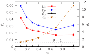
Our results have been derived for systems with underdamped stochastic dynamics. Of greater practical importance in colloidal suspensions is the overdamped limit corresponding to neglecting inertia, $m\rightarrow 0$. In Fig. 7, the dependence of the coefficients on the reduced mass $m$ is plotted. As expected for smaller $m$ the kinetic temperatures approach unity, $\theta_{i}\approx 1$. The additive correction term is no longer negligible as $\beta_{x}$ and $\beta_{y}$ grow. We thus recover the fluctuation-dissipation theorem as described in the introduction, in which the bath temperature enters and the equilibrium form of the FDT is completed by an excess correlation function.

Inserting the overdamped equation of motion for the tagged particle into Eq. (8) one arrives at

$$C_{ij}(t)=2R_{ij}(t)+\langle F^{(1)}_{i}(t)F^{(1)}_{j}(0)\rangle_{0}$$ (31)

for $t>0$ and components $i,j=y,z$ perpendicular to the shear flow Lander et al. (2010). Here, $\mathbf{F}^{(1)}=-\nabla_{1}U$ is the force on the tagged particle exerted by its neighboring particles. The time-integrated version of Eq. (31) has been obtained previously within mode-coupling calculations Szamel (2004); Krüger and Fuchs (2009, 2010). For systems in which the force-force correlations can be neglected Eq. (31) predicts a universal FDR $X_{i}=2$. It has been argued that such an approximation might be justified in dense suspensions close to the glass transition under sufficiently large shear.

Figure 7: (Color online) The coefficients $\beta_{i}$ (solid lines, left axis) and the kinetic temperature $\theta_{x}$ (dashed line, right axis) as a function of the reduced mass $m$ for volume fraction $\phi=0.4$ and strain rate $\dot{\gamma}=2$.

V Summary

We have studied the relation between velocity autocorrelation and response function of a tagged particle moving in a suspension that is driven into a non-equilibrium steady state through simple shear flow. Under the assumption of a time-scale separation between vibrational motion and local reorganization the tagged particle effectively behaves like a trapped particle. The diagonal components of the tagged particle’s velocity autocorrelation function are then given by

$$C_{ii}(t;\dot{\gamma})\approx\theta_{i}(\dot{\gamma})R_{ii}(t;\dot{\gamma})+\dot{\gamma}^{2}\beta_{i}I_{i}(t;\dot{\gamma})$$ (32)

with expansion of the kinetic temperature

$$\theta_{i}(\dot{\gamma})\approx 1+\alpha_{i}\dot{\gamma}^{2}.$$ (33)

Here, $R_{ii}(t;\dot{\gamma})$ are the response functions Eq. (2), $I_{i}(t;\dot{\gamma})$ are functions of order unity, and $\alpha_{i}$ and $\beta_{i}$ are coefficients independent of the strain rate $\dot{\gamma}$. While these expressions are exact for the trapped single particle our numerical results show that they hold approximately to a very good degree for a tagged particle moving in an interacting colloidal suspension. One might of course anticipate the quadratic dependence on strain rate from symmetry arguments close to equilibrium. We have shown here that these expressions follow from a time-scale separation caused by an effective confinement.

The effect of the shear flow is to break symmetry and to couple the particle velocity to earlier perturbations perpendicular to its velocity. This leads to an additive correction term that grows with $\dot{\gamma}^{2}$. Since $\beta_{i}\ll 1$ this correction is negligible up to dimensionless strain rates $\dot{\gamma}\sim(\max\{\beta_{i}\})^{-1/2}$, which can be far from equilibrium. Specifically, here we have studied strain rates in the range $\dot{\gamma}\leqslant 1$ and found excellent agreement between correlation and response functions, see Fig. 3. However, already at $\dot{\gamma}\gtrsim 2$ the kinetic temperatures start to divert from the quadratic law, indicating the importance of higher order terms. Increasing the density the tagged particle interacts more strongly with its surrounding particles. The kinetic temperature increases due to more frequent collisions with neighboring particles in conjunction with transport due to the flow. This is in contrast to the trapped particle where tightening the trap reduces fluctuations and therefore the kinetic temperature approaches the bath temperature.

An intriguing perspective is to apply our results to supercooled (or supersaturated) conditions. Since dynamics slows down dramatically and the time-scale separation between vibrations and long-lived particle displacements becomes even more pronounced we expect that our results extend into the supercooled regime. While we have employed stochastic dynamics one might speculate that our results also hold in systems governed by deterministic dynamics such as the SLLOD equations of motion Tuckerman et al. (1997) as employed in Ref. Berthier and Barrat (2002). Future work will also address the influence of hydrodynamic interactions and flow generated through boundaries.

Appendix A Green’s function for a particle in a harmonic trap in shear flow

The equations of motion (3) for the potential Eq. (11) are most conveniently written as $\dot{\mathbf{x}}\equiv\mathsf{A}\mathbf{x}+(0,\boldsymbol{\xi})^{\text{T}}$ for a vector $\mathbf{x}=(x,y,v_{x},v_{y})^{\text{T}}$ with

$$\mathsf{A}=\frac{1}{m}\left(\begin{array}[]{cccc}0&0&m&0\\ 0&0&0&m\\ -k&\dot{\gamma}&-1&0\\ 0&-k&0&-1\end{array}\right).$$

The Green’s function is

$$\mathsf{G}(t)\equiv e^{\mathsf{A}t}=\left(\begin{array}[]{cc}\mathsf{G}^{rr}(t)&\mathsf{G}^{rv}(t)\\ \mathsf{G}^{vr}(t)&\mathsf{G}^{vv}(t)\end{array}\right).$$

We need the explicit expressions for the following two matrices:

$$\mathsf{G}^{vr}(t)=e^{-t/2m}\left[-\left(\omega+\frac{1}{4m^{2}\omega}\right)\sin\omega t\mathbf{1}+\dot{\gamma}g_{vr}(t)\mathbf{1}_{xy}\right],$$

$$g_{vr}(t)\equiv\frac{(4m^{2}\omega^{2}-1)\sin\omega t+(4m^{2}\omega^{2}+1)\omega t\cos\omega t}{8m^{3}\omega^{3}},$$

$$\mathsf{G}^{vv}(t)=e^{-t/2m}\left[\left(\cos\omega t-\frac{\sin\omega t}{2m\omega}\right)\mathbf{1}+\dot{\gamma}g_{vv}(t)\mathbf{1}_{xy}\right],$$

$$g_{vv}(t)\equiv\frac{(2m\omega^{2}t-1)\sin\omega t+\omega t\cos\omega t}{4m^{2}\omega^{3}},$$

where

$$\omega\equiv\frac{\sqrt{4km-1}}{2m},\qquad\mathbf{1}_{xy}\equiv\left(\begin{array}[]{cc}0&1\\ 0&0\end{array}\right).$$

The diagonal components are independent of the strain rate. To determine $\beta_{x}$ as defined in Eq. (23) we calculate numerically the maximum of $G^{vr}_{xy}(t)$.

For the sake of completeness, the other two matrices are

$$\mathsf{G}^{rr}(t)=e^{-t/2m}\left[\left(\cos\omega t+\frac{\sin\omega t}{2m\omega}\right)\mathbf{1}+\dot{\gamma}g_{rr}(t)\mathbf{1}_{xy}\right],$$

$$g_{rr}(t)\equiv\frac{(2m\omega^{2}t+1)\sin\omega t-\omega t\cos\omega t}{4m^{2}\omega^{3}},$$

$$\mathsf{G}^{rv}(t)=e^{-t/2m}\left[\frac{\sin\omega t}{\omega}\mathbf{1}+\dot{\gamma}g_{rv}(t)\mathbf{1}_{xy}\right],$$

$$g_{rv}(t)\equiv\frac{\sin\omega t-\omega t\cos\omega t}{2m\omega^{3}}.$$

The stationary distribution

$$\psi_{\text{s}}(\mathbf{r},\mathbf{v})=\frac{1}{(2\pi)^{2}\sqrt{\det\mathsf{M}}}\exp\left\{-\frac{1}{2}\mathbf{x}\cdot\mathsf{M}^{-1}\mathbf{x}\right\}$$ (34)

is Gaussian and therefore determined by the symmetric covariance matrix

$$\mathsf{M}\equiv\left(\begin{array}[]{cc}\langle\mathbf{r}\mathbf{r}^{\text{T}}\rangle_{0}&\langle\mathbf{r}\mathbf{v}^{\text{T}}\rangle_{0}\\ \langle\mathbf{v}\mathbf{r}^{\text{T}}\rangle_{0}&\langle\mathbf{v}\mathbf{v}^{\text{T}}\rangle_{0}\end{array}\right)$$

alone. We calculate $\mathsf{M}$ using Chandrasekhar’s theorem Dhont (1996),

$$\mathsf{M}=\frac{2}{m^{2}}\int_{0}^{\infty}\mathrm{d}t\;\left(\begin{array}[]{cc}\mathsf{G}^{rv}(t)\mathsf{G}^{rv\text{T}}(t)&\mathsf{G}^{rv}(t)\mathsf{G}^{vv\text{T}}(t)\\ \mathsf{G}^{vv}(t)\mathsf{G}^{rv\text{T}}(t)&\mathsf{G}^{vv}(t)\mathsf{G}^{vv\text{T}}(t)\end{array}\right).$$

With $1+4(m\omega)^{2}=4km$, we obtain the stationary correlations

$$\langle\mathbf{r}\mathbf{r}^{\text{T}}\rangle_{0}=\frac{1}{k}\mathbf{1}+\frac{1}{2k^{2}}\left(\begin{array}[]{cc}\frac{1+4km}{4k}\dot{\gamma}^{2}&\dot{\gamma}\\ \dot{\gamma}&0\end{array}\right),$$ (37)

$$\langle\mathbf{r}\mathbf{v}^{\text{T}}\rangle_{0}=\frac{1}{2k}\left(\begin{array}[]{cc}0&-\dot{\gamma}\\ \dot{\gamma}&0\end{array}\right),$$ (40)

$$\langle\mathbf{v}\mathbf{v}^{\text{T}}\rangle_{0}=\frac{1}{m}\mathbf{1}+\frac{1}{2k}\left(\begin{array}[]{cc}\dot{\gamma}^{2}&0\\ 0&0\end{array}\right).$$ (43)

The distribution function projected into the configuration space is obtained through integrating out the velocities in the stationary distribution (34),

$$\begin{split}\Psi_{\text{s}}(\mathbf{r})&=\int\mathrm{d}\mathbf{v}\;\psi_{\text{s}}(\mathbf{r},\mathbf{v})\\ &=\frac{1}{2\pi\sqrt{\det\langle\mathbf{r}\mathbf{r}^{\text{T}}\rangle_{0}}}\exp\left\{-\frac{1}{2}\mathbf{r}\cdot\langle\mathbf{r}\mathbf{r}^{\text{T}}\rangle_{0}^{-1}\mathbf{r}\right\}.\end{split}$$

In the overdamped limit one obtains

$$\langle\mathbf{r}\mathbf{r}^{\text{T}}\rangle_{0}\xrightarrow{m\rightarrow 0}\frac{1}{k}\left(\begin{array}[]{cc}1+2\bar{\dot{\gamma}}^{2}&\bar{\dot{\gamma}}\\ \bar{\dot{\gamma}}&1\end{array}\right)$$

with $\bar{\dot{\gamma}}\equiv\dot{\gamma}/2k$.

References

- McQuarrie (2000) D. A. McQuarrie, Statistical Mechanics (University Science Books, Sausalito, 2000).
- Cugliandolo et al. (1997) L. F. Cugliandolo, J. Kurchan, and L. Peliti, Phys. Rev. E 55, 3898 (1997).
- Cugliandolo (2011) L. F. Cugliandolo, arXiv:1104.4901 (2011).
- Kubo et al. (1991) R. Kubo, M. Toda, and N. Hashitsume, Statistical Physics II (Springer-Verlag, Berlin, 1991), 2nd ed.
- Jack et al. (2007) R. L. Jack, M. F. Hagan, and D. Chandler, Phys. Rev. E 76, 021119 (2007).
- Klotsa and Jack (2011) D. Klotsa and R. L. Jack, Soft Matter 7, 6294 (2011).
- Agarwal (1972) G. S. Agarwal, Z. Physik 252, 25 (1972).
- Hänggi and Thomas (1982) P. Hänggi and H. Thomas, Phys. Rep. 88, 207 (1982).
- Crisanti and Ritort (2003) A. Crisanti and F. Ritort, J. Phys. A: Math. Gen. 36, R181 (2003).
- Marconi et al. (2008) U. M. B. Marconi, A. Puglisi, L. Rondoni, and A. Vulpiani, Phys. Rep. 461, 111 (2008).
- Speck and Seifert (2006) T. Speck and U. Seifert, Europhys. Lett. 74, 391 (2006).
- Blickle et al. (2007) V. Blickle, T. Speck, C. Lutz, U. Seifert, and C. Bechinger, Phys. Rev. Lett. 98, 210601 (2007).
- Speck and Seifert (2009) T. Speck and U. Seifert, Phys. Rev. E 79, 040102 (2009).
- Baiesi et al. (2009) M. Baiesi, C. Maes, and B. Wynants, Phys. Rev. Lett. 103, 010602 (2009).
- Prost et al. (2009) J. Prost, J.-F. Joanny, and J. M. R. Parrondo, Phys. Rev. Lett. 103, 090601 (2009).
- Seifert and Speck (2010) U. Seifert and T. Speck, EPL 89, 10007 (2010).
- Speck (2010) T. Speck, Prog. Theor. Phys. Suppl. 184, 248 (2010).
- Ono et al. (2002) I. K. Ono, C. S. O’Hern, D. J. Durian, S. A. Langer, A. J. Liu, and S. R. Nagel, Phys. Rev. Lett. 89, 095703 (2002).
- Hayashi and Sasa (2004) K. Hayashi and S. Sasa, Phys. Rev. E 69, 066119 (2004).
- Haxton and Liu (2007) T. K. Haxton and A. J. Liu, Phys. Rev. Lett. 99, 195701 (2007).
- Berthier and Barrat (2002) L. Berthier and J.-L. Barrat, J. Chem. Phys. 116, 6228 (2002).
- Szamel (2004) G. Szamel, Phys. Rev. Lett. 93, 178301 (2004).
- Krüger and Fuchs (2009) M. Krüger and M. Fuchs, Phys. Rev. Lett. 102, 135701 (2009).
- Lander et al. (2010) B. Lander, U. Seifert, and T. Speck, EPL 92, 58001 (2010).
- Zhang and Szamel (2011) M. Zhang and G. Szamel, Phys. Rev. E 83, 061407 (2011).
- Shukla (2001) P. K. Shukla, Phys. Plasmas 8, 1791 (2001).
- Ziehl et al. (2009) A. Ziehl, J. Bammert, L. Holzer, C. Wagner, and W. Zimmermann, Phys. Rev. Lett. 103, 230602 (2009).
- Calabrese and Gambassi (2005) P. Calabrese and A. Gambassi, J. Phys. A: Math. Gen. 38, R133 (2005).
- Chatelain (2004) C. Chatelain, J. Stat. Mech. p. P06006 (2004).
- Berthier (2007) L. Berthier, Phys. Rev. Lett. 98, 220601 (2007).
- Taylor (1953) G. Taylor, Proc. R. Soc. Lond. A 219, 186 (1953).
- Stillinger and Weber (1984) F. Stillinger and T. Weber, Science 225, 983 (1984).
- Azhar et al. (2000) F. E. Azhar, M. Baus, J.-P. Ryckaert, and E. J. Meijer, J. Chem. Phys. 112, 5121 (2000).
- Allen and Tildesley (1987) M. P. Allen and D. J. Tildesley, Computer Simulation of Liquids (Clarendon Press, Oxford, 1987).
- Frenkel and Smit (2002) D. Frenkel and B. Smit, Understanding Molecular Simulation: From Algorithms to Applications (Academic Press, San Diego, 2002), 2nd ed.
- Strating (1999) P. Strating, Phys. Rev. E 59, 2175 (1999).
- Foss and Brady (2000) D. R. Foss and J. F. Brady, J. Rheol. 44, 629 (2000).
- Krüger and Fuchs (2010) M. Krüger and M. Fuchs, Prog. Theor. Phys. Supplement 184, 172 (2010).
- Tuckerman et al. (1997) M. E. Tuckerman, C. J. Mundy, S. Balasubramanian, and M. L. Klein, J. Chem. Phys. 106, 5615 (1997).
- Dhont (1996) J. K. G. Dhont, An Introduction to Dynamics of Colloids (Elsevier, Amsterdam, 1996).