Abstract

We compute the Hochschild homology and cohomology, and cyclic homology, of almost Calabi-Yau algebras for $SU(3)$ $\mathcal{ADE}$ graphs. These almost Calabi-Yau algebras are a higher rank analogue of the pre-projective algebras for Dynkin diagrams, which are $SU(2)$-related constructions. The Hochschild (co)homology and cyclic homology of $A$ can be regarded as invariants for the braided subfactors associated to the $SU(3)$ modular invariants.

1 Introduction

The classical McKay correspondence appears in various contexts. It relates finite subgroups $\Gamma$ of $SU(2)$ with the algebraic geometry of the quotient Kleinian singularities $\mathbb{C}^{2}/\Gamma$ [33] but also with the classification of $SU(2)$ modular invariants and quantum subgroups of $SU(2)$ [8, 40, 31, 32, 37, 1, 2, 4, 5].

Minimal resolutions of Kleinian singularities can be described via the moduli space of representations of the preprojective algebra associated to the action of $\Gamma$ [12]. Preprojective algebras associated to graphs were introduced in [25], and it was shown that they are finite dimensional if and only if the graphs are of $ADE$ type, that is, one of the simply laced Dynkin diagrams. The preprojective algebra $A$ for an $ADE$ Dynkin diagram is a Frobenius algebra, that is, there is a linear function $f:A\rightarrow\mathbb{C}$ such that $(x,y):=f(xy)$ is a non-degenerate bilinear form (this is equivalent to the statement that $A$ is isomorphic to its dual $\widehat{A}=\mathrm{Hom}(A,\mathbb{C})$ as left (or right) $A$-modules). There is an automorphism $\beta$ of $A$, called the Nakayama automorphism of $A$ (associated to $f$), such that $(x,y)=(y,\beta(x))$, which yields an $A$-$A$ bimodule isomorphism $\widehat{A}\rightarrow{}_{1}A_{\beta}$ [39]. The Nakayama automorphism for each $ADE$ graph was determined in [13, 14] (see also [7]). The preprojective algebra $A$ has a finite resolution as an $A$-$A$ bimodule, which was used by Erdmann and Snashall to determine the Hochschild cohomology $HH^{\bullet}(A)$ of $A$ for the $ADE$ graphs $A_{n}$, along with its ring structure [13], and $HH^{2}(A)$ for the graphs $D_{n}$ [14] This finite resolution yields a projective resolution of $A$ as an $A$-$A$ bimodule, which was used by Etingof and Eu to determine the Hochschild homology and cohomology, and cyclic homology, of $A$ for all $ADE$ Dynkin diagrams [15], along with the ring structure of the Hochschild cohomology [17]. The Hochschild homology and cohomology, cyclic homology, and ring structure of the Hochschild cohomology, for the preprojective algebra for the tadpole graphs $T_{n}$ were obtained in [18]. The Hochschild homology and cohomology for the case of the affine Dynkin diagrams, which are the McKay graphs for the finite subgroups of $SU(2)$, were determined in [11].

More generally, one tries to understand singularities via a noncommutative algebra $A$, often called a noncommutative resolution, whose centre corresponds to the coordinate ring of the singularity [35]. The algebra should be finitely generated over its centre, and the desired favourable resolution is the moduli space of representations of $A$, whose category of finitely generated modules is derived equivalent to the category of coherent sheaves of the resolution. In the case of a quotient singularity $\mathbb{C}^{3}/\Gamma$ for a finite subgroup $\Gamma$ of $SU(3)$, the corresponding noncommutative algebra $A$ is a Calabi-Yau algebra of dimension 3.

Calabi-Yau algebras arise naturally in the study of Calabi-Yau manifolds, providing a noncommutative version of conventional Calabi-Yau geometry. An algebra $A$ is Calabi-Yau of dimension $n$ if the bounded derived category of the abelian category of finite dimensional $A$-modules is a Calabi-Yau category of dimension $n$. In this case the global dimension of $A$ is $n$ [6]. The derived category of coherent sheaves over an $n$-dimensional Calabi-Yau manifold is a Calabi-Yau category of dimension $n$ and they appear naturally in the study of boundary conditions of the $B$-model in superstring theory over the manifold. For more on Calabi-Yau algebras, see e.g. [6, 26].

In [26, Remark 4.5.7] Ginzburg introduced, in his terminology, $q$-deformed Calabi-Yau algebras. In the case where $q$ is not a root of unity, these algebras are Calabi-Yau algebras of dimension 3. We study these algebras in the case where $q$ is a root of unity, which are the $SU(3)$ generalizations of preprojective algebras for the Coxeter-Dynkin diagrams $ADE$. We call these algebras almost Calabi-Yau algebras. In a recent work [23], we determined the Nakayama automorphism for each $\mathcal{ADE}$ graph, and constructed a finite resolution of $A$ as an $A$-$A$ bimodule, see (5).

Our interest in these almost Calabi-Yau algebras came from subfactor theory, and in particular, braided subfactors of von Neumann algebras, which provide a framework for studying two dimensional conformal field theories and their modular invariant partition functions. In the case of Wess-Zumino-Witten models associated to $SU(n)$ at level $k$, the Verlinde algebra is a non-degenerately braided system of endomorphisms ${}_{N}\mathcal{X}_{N}$, labelled by the positive energy representations of the loop group of $SU(n)_{k}$ on a type $\mathrm{III}_{1}$ factor $N$, with fusion rules $\lambda\mu=\bigoplus_{\nu}N_{\lambda\nu}^{\mu}\nu$ which exactly match those of the positive energy representations [36]. The fusion matrices $N_{\lambda}=[N_{\rho\lambda}^{\sigma}]_{\rho,\sigma}$ are a family of commuting normal matrices which give a representation themselves of the fusion rules of the positive energy representations of the loop group of $SU(n)_{k}$, $N_{\lambda}N_{\mu}=\sum_{\nu}N_{\lambda\nu}^{\mu}N_{\nu}$. This family $\{N_{\lambda}\}$ of fusion matrices can be simultaneously diagonalised:

$$N_{\lambda}=\sum_{\sigma}\frac{S_{\sigma,\lambda}}{S_{\sigma,0}}S_{\sigma}S_{\sigma}^{\ast},$$

where $0$ is the trivial representation, and the eigenvalues $S_{\sigma,\lambda}/S_{\sigma,0}$ and eigenvectors $S_{\sigma}=[S_{\sigma,\mu}]_{\mu}$ are described by the statistics $S$ matrix. The key structure in the conformal field theory is the modular invariant partition function $Z$. In the subfactor setting this is realised by a braided subfactor $N\subset M$ where trivial (or permutation) invariants in the ambient factor $M$ when restricted to $N$ yield $Z$. This would mean that the dual canonical endomorphism is in $\Sigma({}_{N}\mathcal{X}_{N})$, i.e. decomposes as a finite linear combination of endomorphisms in ${}_{N}\mathcal{X}_{N}$. Indeed if this is the case for the inclusion $N\subset M$, then the process of $\alpha$-induction allows us to analyse the modular invariant, providing two extensions of $\lambda$ on $N$ to endomorphisms $\alpha^{\pm}_{\lambda}$ of $M$, such that the matrix $Z_{\lambda,\mu}=\langle\alpha_{\lambda}^{+},\alpha_{\mu}^{-}\rangle$ is a modular invariant [4, 3, 20]. The action of the system ${}_{N}\mathcal{X}_{N}$ on the $N$-$M$ sectors ${}_{N}\mathcal{X}_{M}$ produces a nimrep (non-negative matrix integer representation of the fusion rules) $G_{\lambda}G_{\mu}=\sum_{\nu}N_{\lambda\nu}^{\mu}G_{\nu}$, whose spectrum reproduces exactly the diagonal part of the modular invariant, i.e.

$$G_{\lambda}=\sum_{\sigma}\frac{S_{\sigma,\lambda}}{S_{\sigma,0}}\psi_{\sigma}\psi_{\sigma}^{\ast},$$

with the spectrum of $G_{\lambda}$ given by $G_{\lambda}=\{S_{\mu,\lambda}/S_{\mu,0}\textrm{ with multiplicity }Z_{\mu,\mu}\}$ [5, Theorem 4.16].

The systems ${}_{N}\mathcal{X}_{N}$, ${}_{N}\mathcal{X}_{M}$, ${}_{M}\mathcal{X}_{M}$ are (the irreducible objects of) tensor categories of endomorphisms with the Hom-spaces as their morphisms. Thus ${}_{N}\mathcal{X}_{N}$ gives a braided modular tensor category, and ${}_{N}\mathcal{X}_{M}$ a module category.

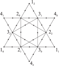
Figure 6: Graph $\mathcal{E}^{(8)}$

In our work we have focused on braided subfactors associated to $SU(3)$ modular invariants, which are labeled by a family of graphs which we call the $SU(3)$ $\mathcal{ADE}$ graphs. The complete list of the $SU(3)$ $\mathcal{ADE}$ graphs are illustrated in [24, Figures 5-9]. For positive integer $k<\infty$ we have a braided modular tensor category ${}_{N}\mathcal{X}_{N}=\{\lambda_{(p,l)}|\;0\leq p,l,p+l\leq k\}$, a non-degenerately braided system of endomorphisms on a type $\mathrm{III}_{1}$ factor $N$, which is generated by $\rho=\lambda_{(1,0)}$ and its conjugate $\overline{\rho}=\lambda_{(0,1)}$, where the irreducible endomorphisms $\lambda_{(p,l)}$ satisfy the fusion rules of $SU(3)_{k}$:

$$\lambda_{(p,l)}\otimes\rho\cong\lambda_{(p,l-1)}\oplus\lambda_{(p-1,l+1)}\oplus\lambda_{(p+1,l)},\quad\lambda_{(p,l)}\otimes\overline{\rho}\cong\lambda_{(p-1,l)}\oplus\lambda_{(p+1,l-1)}\oplus\lambda_{(p,l+1)},$$ (1)

where $\lambda_{(p^{\prime},l^{\prime})}$ is understood to be zero if $p^{\prime}<0$, $l^{\prime}<0$ or $p^{\prime}+l^{\prime}\geq k+1$. Then a pair $(\mathcal{G},W)$, of a cell system $W$ (see Section 2) on an $SU(3)$ $\mathcal{ADE}$ graph $\mathcal{G}$ with Coxeter number $k+3$ yields a braided subfactor $N\subset M$ and a module category ${}_{N}\mathcal{X}_{M}$, where the associated modular invariant, labeled by $\mathcal{G}$, is at level $k$. For such a braided subfactor, the almost Calabi-Yau algebra can be constructed via a monoidal functor $F$, which is essentially the module category ${}_{N}\mathcal{X}_{M}$, from the $A_{2}$-Temperley-Lieb category to the category $\mathrm{Fun}({}_{N}\mathcal{X}_{M},{}_{N}\mathcal{X}_{M})$ of additive functors from ${}_{N}\mathcal{X}_{M}$ to itself.

The $A_{2}$-Temperley-Lieb category constructed in [23] used ideas from planar algebras, and in particular, the $A_{2}$-planar algebras of [22] (see also an earlier construction of the $A_{2}$-Temperley-Lieb category in [10], and of the Temperley-Lieb category in [34, 38]).

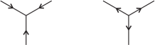
Figure 1: $A_{2}$ webs

For $m_{i},n_{i}\geq 0$, an $A_{2}$-$(m_{2},n_{2}),(m_{1},n_{1})$-tangle $T$ is a tangle on an rectangle with $m_{2}+n_{2}$, $m_{1}+n_{1}$ vertices along the top, bottom edges respectively, generated by $A_{2}$ webs (see Figure 1) such that every free end of $T$ is attached to a vertex along the top or bottom of the rectangle in a way that respects the orientation of the strings, every vertex has a string attached to it, and the tangle contains no elliptic faces. We call a vertex a source vertex if the string attached to it has orientation away from the vertex. Similarly, a sink vertex will be a vertex where the string attached has orientation towards the vertex. Along the top, bottom edge the first $m_{i}$ vertices are source, sink vertices respectively, and the last $n_{i}$ are sink, source vertices respectively. Let $V^{A_{2}}_{(m_{2},n_{2}),(m_{1},n_{1})}$ be the quotient of the free vector space over $\mathbb{C}$ with basis the $A_{2}$-$(m_{2},n_{2}),(m_{1},n_{1})$-tangles, by the Kuperberg ideal generated by the Kuperberg relations K1-K3 [28]. Then at level $k$, the $A_{2}$-Temperley-Lieb category is defined to be a quotient of the category $A_{2}\textrm{-}TL=\mathrm{Mat}(C^{A_{2}})$ by the negligible morphisms, where $C^{A_{2}}$ is the tensor category whose objects are projections in $V^{A_{2}}_{(m,n),(m,n)}$ and whose morphisms are $\mathrm{Hom}(p_{1},p_{2})=p_{2}V^{A_{2}}_{(m_{2},n_{2}),(m_{1},n_{1})}p_{1}$, for projections $p_{i}\in V^{A_{2}}_{(m_{i},n_{i}),(m_{i},n_{i})}$, $i=1,2$. We write $A_{2}\textrm{-}TL_{(m,n)}=V^{A_{2}}_{(m,n),(m,n)}$, and $\rho$, $\overline{\rho}$ for the identity projections in $A_{2}\textrm{-}TL_{(1,0)}$, $A_{2}\textrm{-}TL_{(0,1)}$ respectively consisting of a single string with orientation downwards, upwards respectively. Then the identity diagram in $A_{2}\textrm{-}TL_{(m,n)}$, given by $m+n$ vertical strings where the first $m$ strings have downwards orientation and the next $n$ have upwards orientation, is expressed as $\rho^{m}\overline{\rho}^{n}$. It is a linear combination of simple projections $f_{(i,j)}$ for $i,j\geq 0$, $0\leq i+j<m+n$ such that $i-j\cong m-n\textrm{ mod }3$, and a simple projection $f_{(m,n)}$, where $f_{(1,0)}=\rho$, $f_{(0,1)}=\overline{\rho}$ and $f_{(0,0)}$ is the empty diagram. The morphisms $\mathfrak{f}_{(p,l)}=\mathrm{id}_{f_{(p,l)}}$ are generalized Jones-Wenzl projections. The $f_{(p,l)}$ satisfy the fusion rules for $SU(3)$ [23]:

$$f_{(p,l)}\otimes\rho\cong f_{(p,l-1)}\oplus f_{(p-1,l+1)}\oplus f_{(p+1,l)},\quad f_{(p,l)}\otimes\overline{\rho}\cong f_{(p-1,l)}\oplus f_{(p+1,l-1)}\oplus f_{(p,l+1)}.$$ (2)

At level $k$, the negligible morphisms are the ideal $\langle\mathfrak{f}_{(p,l)}|p+l=k+1\rangle$ generated by $\mathfrak{f}_{(p,l)}$ such that $p+l=k+1$. The $A_{2}$-Temperley-Lieb category is the quotient $A_{2}\textrm{-}TL^{(k)}:=A_{2}\textrm{-}TL/\langle\mathfrak{f}_{(p,l)}|p+l=k+1\rangle$, which is semisimple with simple objects $f_{(p,l)}$, $p,l\geq 0$ such that $p+l\leq k$ which satisfy the fusion rules (1) of $SU(3)_{k}$, that is we have (2) where $f_{(p^{\prime},l^{\prime})}$ is understood to be zero if $p^{\prime}<0$, $l^{\prime}<0$ or $p^{\prime}+l^{\prime}\geq k+1$. The $A_{2}$-Temperley-Lieb category $A_{2}\textrm{-}TL^{(k)}$ may be identified with the braided modular tensor category ${}_{N}\mathcal{X}_{N}$, where the object $f_{(p,l)}\in A_{2}\textrm{-}TL^{(k)}$ is identified with $\lambda_{(p,l)}\in{}_{N}\mathcal{X}_{N}$.

Then the monoidal functor $F$ is given on the simple objects $f_{(p,l)}$ of $A_{2}\textrm{-}TL^{(k)}$ by

$$F(f_{(p,l)})=\bigoplus_{i,j\in\mathcal{G}_{0}}G_{\lambda_{(p,l)}}(i,j)\,\mathbb{C}_{i,j},$$ (3)

where $\mathbb{C}_{i,j}$ are 1-dimensional $R$-$R$ bimodules, where $R=(\mathbb{C}\mathcal{G})_{0}$. The category of $R$-$R$ bimodules has a natural monoidal structure given by $\otimes_{R}$. The functor $F$ is defined on the morphisms of $A_{2}\textrm{-}TL^{(k)}$ using the cell system $W$ and the Perron-Frobenius eigenvector of $\mathcal{G}$, see [23, Section 2.9].

If $\mathcal{G}^{\mathrm{op}}$ denotes the opposite graph of $\mathcal{G}$ obtained by reversing the orientation of every edge of $\mathcal{G}$, we have that $F(\rho^{m}\overline{\rho}^{n})$ is the $R$-$R$ bimodule with basis given by all paths of length $m+n$ on $\mathcal{G}$, $\mathcal{G}^{\mathrm{op}}$, where the first $m$ edges are on $\mathcal{G}$ and the last $n$ edges are on $\mathcal{G}^{\mathrm{op}}$. In particular $F(\rho^{m})=(\mathbb{C}\mathcal{G})_{m}$, so that we have the graded algebra $\bigoplus_{m}F(\rho^{m})=(\mathbb{C}\mathcal{G})$, the path algebra of $\mathcal{G}$. The endomorphisms $\rho^{m}$ are not irreducible however, but decompose into direct sums of the generalized Jones-Wenzl projections $f_{(p,0)}$. The natural algebra to consider is thus the graded algebra $\Sigma=\bigoplus_{j}F(f_{(j,0)})$, where the $p^{\mathrm{th}}$ graded part is $\Sigma_{p}=F(f_{(p,0)})$. The multiplication $\mu$ is defined by $\mu_{p,l}=F(\mathfrak{f}_{(p+l,0)}):\Sigma_{p}\otimes_{R}\Sigma_{l}\rightarrow\Sigma_{p+l}$, where $\mathfrak{f}_{(p,l)}=\mathrm{id}_{f_{(p,l)}}$. The graded algebra $\Sigma$ is isomorphic to the almost Calabi-Yau algebra $A=A(\mathcal{G},W)$ [10, 23].

In Section 2 we introduce the almost Calabi-Yau algebra $A=A(\mathcal{G},W)$ for a pair $(\mathcal{G},W)$ of a cell system $W$ on an $SU(3)$ $\mathcal{ADE}$ graph $\mathcal{G}$. Then in Section 2.1 we determine a periodic projective resolution of $A$ as an $A$-$A$ bimodule, starting from the finite resolution of $A$ determined in [23, Theorem 5.1], which will be used to determine the Hochschild (co)homology and cyclic homology of $A$ in Sections 3-4. In Section 3.1 we use the projective resolution determined in Section 2.1 to construct a Hochschild homology complex for $A$, and introduce the cyclic homology of $A$ in Section 3.2. We then determine the Hochschild and cyclic homology of $A$ in Sections 3.3-3.5 for the graphs $\mathcal{A}^{(n)}$, $n=4,5,6,7$, $\mathcal{D}^{(3k+3)}$, $k\geq 1$, $\mathcal{A}^{(n)\ast}$, $n\geq 5$, $\mathcal{D}^{(3k)\ast}$, $k\geq 2$, $\mathcal{E}^{(8)}$ and $\mathcal{E}^{(8)\ast}$. Finally in Section 4 we construct a Hochschild cohomology complex for $A$ and use this to determine the Hochschild cohomology of $A$ in the cases listed above.

The Hochschild (co)homology and cyclic homology of $A$ can be regarded as invariants for the braided subfactors associated to the $SU(3)$ modular invariants. Beginning with a pair $(\mathcal{G},W)$ given by a cell system $W$ on an $SU(3)$ $\mathcal{ADE}$ graph $\mathcal{G}$, we construct a braided subfactor $N\subset M$ which yields a nimrep which recovers the graph $\mathcal{G}$ as described above. Then we can construct the algebra $A(\mathcal{G},W)$ whose Hochschild (co)homology and cyclic homology only depends on the original pair $(\mathcal{G},W)$, or equivalently, on the braided subfactor $N\subset M$.

2 Almost Calabi-Yau algebras

Let $\mathcal{G}$ be a finite directed graph, and denote by $\mathcal{G}_{n}$ the set of all paths on $\mathcal{G}$ of length $n$. The vertices of $\mathcal{G}$ are the paths of length 0. If $a\in\mathcal{G}_{1}$ is an edge on $\mathcal{G}$, we denote by $\widetilde{a}\in\mathcal{G}^{\mathrm{op}}_{1}$ the corresponding edge with opposite orientation on $\mathcal{G}^{\mathrm{op}}$. The path algebra $\mathbb{C}\mathcal{G}=\bigoplus_{k=0}^{\infty}(\mathbb{C}\mathcal{G})_{k}$ is the graded complex vector space with basis of the $k^{\mathrm{th}}$-graded part $(\mathbb{C}\mathcal{G})_{k}$ given by $\mathcal{G}_{k}$, where paths may begin at any vertex of $\mathcal{G}$. Multiplication of two paths $a\in(\mathbb{C}\mathcal{G})_{k}$ and $b\in(\mathbb{C}\mathcal{G})_{l}$ is given by concatenation of paths $a\cdot b\in(\mathbb{C}\mathcal{G})_{k+l}$ (or simply $ab$), with $ab$ defined to be zero if $r(a)\neq s(b)$, where $s(a)$, $r(a)$ denotes the source, range vertex respectively of the path $a$. The commutator quotient $\mathbb{C}\mathcal{G}/[\mathbb{C}\mathcal{G},\mathbb{C}\mathcal{G}]$ may be identified, up to cyclic permutation of the arrows, with the vector space spanned by cyclic paths in $\mathcal{G}$. Let $\partial_{a}:\mathbb{C}\mathcal{G}/[\mathbb{C}\mathcal{G},\mathbb{C}\mathcal{G}]\rightarrow\mathbb{C}\mathcal{G}$ be the derivation given by $\partial_{a}(a_{1}\cdots a_{n})=\sum_{j}a_{j+1}\cdots a_{n}a_{1}\cdots a_{j-1}$, where the summation is over all indices $j$ such that $a_{j}=a$. Then for a potential $\Phi\in\mathbb{C}\mathcal{G}/[\mathbb{C}\mathcal{G},\mathbb{C}\mathcal{G}]$, which is some linear combination of cyclic paths in $\mathcal{G}$, we define the algebra $A(\mathbb{C}\mathcal{G},\Phi)=\mathbb{C}\mathcal{G}/\{\partial_{a}\Phi\}$, which is the quotient of the path algebra by the two-sided ideal generated by the relations $\partial_{a}\Phi\in\mathbb{C}\mathcal{G}$, for all edges $a$ of $\mathcal{G}$. The Hilbert series $H_{A}$ for $A(\mathbb{C}\mathcal{G},\Phi)$ is defined as $H_{A}(t)=\sum_{k=0}^{\infty}H_{ji}^{k}t^{k}$, where the $H_{ji}^{k}$ are matrices which count the dimension of the subspace $\{ixj|\;x\in A(\mathbb{C}\mathcal{G},\Phi)_{k}\}$, where $A(\mathbb{C}\mathcal{G},\Phi)_{k}$ is the subspace of $A(\mathbb{C}\mathcal{G},\Phi)$ of all paths of length $k$, and $i,j\in A(\mathbb{C}\mathcal{G},\Phi)_{0}$.

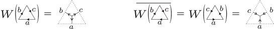
Figure 2: Cells associated to trivalent vertices

Ocneanu [31] defined a cell system $W$ on any $SU(3)$ $\mathcal{ADE}$ graph $\mathcal{G}$, associating a complex number $W\left(\triangle_{i,j,k}^{(a,b,c)}\right)$, now called an Ocneanu cell, to each closed loop of length three $\triangle_{i,j,k}^{(a,b,c)}$ in $\mathcal{G}$ as in Figure 2, where $a,b,c$ are edges on $\mathcal{G}$, and $i,j,k$ are the vertices on $\mathcal{G}$ given by $i=s(a)=r(c)$, $j=s(b)=r(a)$, $k=s(c)=r(b)$. These cells satisfy two properties, called Ocneanu’s type I, II equations respectively, which are obtained by evaluating the Kuperberg relations K2, K3 for an $A_{2}$-spider [28] using the identification in Figure 2:
$(i)$ for any type I frame in $\mathcal{G}$ we have

$$\sum_{k,b_{1},b_{2}}W\left(\triangle_{i,j,k}^{(a,b_{1},b_{2})}\right)\overline{W\left(\triangle_{i,j,k}^{(a^{\prime},b_{1},b_{2})}\right)}=\delta_{a,a^{\prime}}[2]_{q}\phi_{i}\phi_{j}$$

$(ii)$ for any type II frame in $\mathcal{G}$ we have

$$\sum_{k,b_{j}}\phi_{k}^{-1}W\left(\triangle_{i_{2},i_{1},k}^{(a_{2},b_{1},b_{2})}\right)\overline{W\left(\triangle_{i_{2},i_{3},k}^{(a_{3},b_{3},b_{2})}\right)}W\left(\triangle_{i_{4},i_{3},k}^{(a_{4},b_{3},b_{4})}\right)\overline{W\left(\triangle_{i_{4},i_{1},k}^{(a_{1},b_{4},b_{1})}\right)}$$

$$=\delta_{a_{1},a_{4}}\delta_{a_{2},a_{3}}\phi_{i_{4}}\phi_{i_{1}}\phi_{i_{2}}+\delta_{a_{1},a_{2}}\delta_{a_{3},a_{4}}\phi_{i_{1}}\phi_{i_{2}}\phi_{i_{3}}\hskip 71.13188pt$$

Here $(\phi_{v})_{v}$ is the Perron-Frobenius eigenvector for the Perron-Frobenius eigenvalue $\alpha=[3]_{q}$ of $\mathcal{G}$. The existence of these cells for the finite $\mathcal{ADE}$ graphs was claimed by Ocneanu [31], and shown in [21] with the exception of the graph $\mathcal{E}_{4}^{(12)}$. These cells define a unitary connection on the graph $\mathcal{G}$ which satisfy the Yang-Baxter equation [21, Lemma 3.2].

Two cell systems $W_{1}$, $W_{2}$ on an $SU(3)$ $\mathcal{ADE}$ graph $\mathcal{G}$ are equivalent if, for each pair of adjacent vertices $i$, $j$ of $\mathcal{G}$, we can find a family of unitary matrices $(u(a,b))_{a,b}$, where $a$, $b$ are any pair of edges from $i$ to $j$, such that

$$W_{1}(\triangle_{i_{1},i_{2},i_{3}}^{(a_{1},a_{2},a_{3})})=\sum_{a_{1}^{\prime},a_{2}^{\prime},a_{3}^{\prime}}u(a_{1},a_{1}^{\prime})u(a_{2},a_{2}^{\prime})u(a_{3},a_{3}^{\prime})W_{2}(\triangle_{i_{1},i_{2},i_{3}}^{(a_{1}^{\prime},a_{2}^{\prime},a_{3}^{\prime})}),$$

where $a_{l}$ are edges from $i_{l}$ to $i_{l+1}$, and the sum is over all edges $a_{l}^{\prime}$ from $i_{l}$ to $i_{l+1}$, $l=1,2,3$.

There is up to equivalence precisely one connection on the graphs $\mathcal{A}^{(m)}$, $\mathcal{A}^{(2m+1)\ast}$, $\mathcal{E}^{(8)}$, $\mathcal{E}^{(8)\ast}$, $\mathcal{E}_{5}^{(12)}$ and $\mathcal{E}^{(24)}$. For the graphs $\mathcal{A}^{(2m)\ast}$ and $\mathcal{E}_{2}^{(12)}$ there are precisely two inequivalent connections, which are obtained from each other by a $\mathbb{Z}_{2}$ symmetry of the graph. This $\mathbb{Z}_{2}$ symmetry is the conjugation of the graph in the case of $\mathcal{E}_{2}^{(12)}$. There is at least one connection for each graph $\mathcal{D}^{(m)}$, $m\not\equiv 0\textrm{ mod }3$, and at least two inequivalent connections for each graph $\mathcal{D}^{(3p)}$, which are the complex conjugates of each other. There is at least one connection for each graph $\mathcal{D}^{(2m+1)\ast}$, and at least two inequivalent connections for each graph $\mathcal{D}^{(2m)\ast}$, which are obtained from each other by a $\mathbb{Z}_{2}$ symmetry of the graph. There are also at least two inequivalent connections for the graph $\mathcal{E}_{1}^{(12)}$, which are obtained from each other by conjugation of the graph.

For the $SU(3)$ $\mathcal{ADE}$ graphs, we define the almost Calabi-Yau algebra $A(\mathcal{G},W)$ to be the graded quotient algebra

$$A(\mathcal{G},W):=A(\mathbb{C}\mathcal{G},\Phi_{W}),$$

where the potential $\Phi_{W}$ is given by [23, equation (40)] (see also [26, Remark 4.5.7]):

$$\Phi_{W}=\sum_{abc}W(\triangle_{abc})\triangle_{abc}\quad\in\mathbb{C}\mathcal{G}/[\mathbb{C}\mathcal{G},\mathbb{C}\mathcal{G}],$$

where the summation is over all closed paths $abc$ of length 3 on $\mathcal{G}$. The grading on $\mathbb{C}\mathcal{G}$ descends to the quotient algebra $A=A(\mathcal{G},W)$. These almost Calabi-Yau algebras were studied in [23] for all the cell systems constructed in [21]. Equivalent cell systems yield isomorphic almost Calabi-Yau algebras. For any cell system $W$, we can take its complex conjugate $\overline{W}$ to obtain another (possibly equivalent) cell system. The almost Calabi-Yau algebra for $\overline{W}$ is isomorphic to that for $W$. The conjugation $\tau:{}_{N}\mathcal{X}_{N}\rightarrow{}_{N}\mathcal{X}_{N}$ on the braided system of endomorphisms of $SU(3)_{k}$ on a factor $N$, given by the conjugation on the representations of $SU(3)$, induces a conjugation $\tau:{}_{N}\mathcal{X}_{M}\rightarrow{}_{N}\mathcal{X}_{M}$ such that $G_{\overline{\lambda}}=\tau G_{\lambda}\tau$, where $G_{\lambda}a=\lambda a$ for $\lambda\in{}_{N}\mathcal{X}_{N}$, $a\in{}_{N}\mathcal{X}_{M}$. For any cell system $W=W^{+}$, this conjugation of the graph yields a conjugate cell system $W^{-}$, which might be equivalent to $W^{+}$. The almost Calabi-Yau algebra for $W^{-}$ is anti-isomorphic to that for $W^{+}$.

The Hilbert series $H_{A}(t)$ of $A(\mathcal{G},W)$, for an $SU(3)$ $\mathcal{ADE}$ graph $\mathcal{G}$ with adjacency matrix $\Delta_{\mathcal{G}}$, Coxeter number $h=k+3$ and cell system $W$, is given by [23, Theorem 3.1]

$$H_{A}(t)=\frac{1-Pt^{h}}{1-\Delta_{\mathcal{G}}t+\Delta_{\mathcal{G}}^{T}t^{2}-t^{3}},$$ (4)

where $P$ is the permutation matrix corresponding to a $\mathbb{Z}_{3}$ symmetry of the graph. It is the identity for $\mathcal{D}^{(n)}$, $\mathcal{A}^{(n)\ast}$, $n\geq 5$, $\mathcal{E}^{(8)\ast}$, $\mathcal{E}_{l}^{(12)}$, $l=1,2,4,5$, and $\mathcal{E}^{(24)}$. For the remaining graphs $\mathcal{A}^{(n)}$, $\mathcal{D}^{(n)\ast}$ and $\mathcal{E}^{(8)}$, let $V$ be the permutation matrix corresponding to the clockwise rotation of the graph by $2\pi/3$. Then

$$P=\left\{\begin{array}[]{cl}V^{2}&\mbox{ for }\quad\mathcal{A}^{(n)},n\geq 4,\\ V&\mbox{ for }\quad\mathcal{E}^{(8)},\\ V^{2n}&\mbox{ for }\quad\mathcal{D}^{(n)\ast},n\geq 5.\end{array}\right.$$

The numerator and denominator in (4) commute, since any permutation matrix which corresponds to a symmetry of the graph $\mathcal{G}$ commutes with $\Delta_{\mathcal{G}}$ and $\Delta_{\mathcal{G}}^{T}$.

2.1 Periodic resolution for almost Calabi-Yau algebras

We define a non-degenerate form on $A$ by setting $f$ to be the function which is 0 on every element of $A$ of length $<h-3$, and 1 on $u_{i\nu(i)}$ for some $i\in\mathcal{G}_{1}$, where $u_{j\nu(j)}$ denotes a generator of the one-dimensional top-degree space $j\cdot A_{h-3}\cdot\nu(j)$, where $\nu$ is the permutation of the vertices of $\mathcal{G}$ given by the permutation matrix $P$ in (4). Then using the relation $(x,y)=(y,\beta(x))$ this determines the value of $f$ on $u_{j\nu(j)}$, for all other $j\in\mathcal{G}_{1}$. We normalize the $u_{j\nu(j)}$ such that $f(u_{j\nu(j)})=1$ for all $j\in\mathcal{G}_{1}$. The image of the simple object $f_{(k,0)}\in A_{2}\textrm{-}TL^{(k)}$ under the functor $F$ given by (3) defines a unique permutation $\nu$ of the graph $\mathcal{G}$, which is described as follows. The permutation $\nu$ of the graph is given by the $\mathbb{Z}_{3}$ symmetry which defines the permutation matrix $P$ in (4) (note that there are no double edges on the graphs $\mathcal{G}$ for which $P$ is non-trivial). Then the Nakayama automorphism $\beta$ of $A$ is defined on $\mathcal{G}$ by $\beta=\nu$ [23, Theorem 4.6].

Now $A$ has the following finite resolution as an $A$-$A$ bimodule [23, Theorem 5.1]:

$$0\rightarrow\mathcal{N}[h]\stackrel{{\scriptstyle\iota_{0}}}{{\rightarrow}}A\otimes_{S}A[3]\stackrel{{\scriptstyle\mu_{3}}}{{\rightarrow}}A\otimes_{S}\widetilde{V}\otimes_{S}A[1]\stackrel{{\scriptstyle\mu_{2}}}{{\rightarrow}}A\otimes_{S}V\otimes_{S}A\stackrel{{\scriptstyle\mu_{1}}}{{\rightarrow}}A\otimes_{S}A\stackrel{{\scriptstyle\mu_{0}}}{{\rightarrow}}A\rightarrow 0.$$ (5)

Here $S$ is the $A$-$A$ bimodule $(\mathbb{C}\mathcal{G})_{0}$, and $V$, $\widetilde{V}$ are the $A$-$A$ bimodules generated by $\mathcal{G}_{1}$, $\mathcal{G}^{\mathrm{op}}_{1}$ respectively. The $A$-$A$ bimodule $\mathcal{N}={}_{1}A_{\beta^{-1}}$ is equal to $A$ as a vector space. The left $A$-action is given by concatenation, but the right $A$-action is twisted by the inverse of the Nakayama automorphism $\beta$, i.e. $a\cdot x\cdot b=ax\beta^{-1}(b)$ for all $a,b\in A$, $x\in\mathcal{N}$. The connecting $A$-$A$ bimodule maps are given by

$$\mu_{0}(1\otimes 1) = 1,$$ (6)

$$\mu_{1}(1\otimes a\otimes 1) = a\otimes 1-1\otimes a,$$ (7)

$$\mu_{2}(1\otimes\widetilde{a}\otimes 1) = \sum_{b,b^{\prime}\in\mathcal{G}_{1}}W_{abb^{\prime}}(b\otimes b^{\prime}\otimes 1+1\otimes b\otimes b^{\prime}),$$ (8)

$$\mu_{3}(1\otimes 1) = \sum_{a\in\mathcal{G}_{1}}a\otimes\widetilde{a}\otimes 1-\sum_{a\in\mathcal{G}_{1}}1\otimes\widetilde{a}\otimes a,$$ (9)

$$\iota_{0}(1) = \sum_{j}w_{j}\otimes w_{j}^{\ast},$$

where $\{w_{j}\}$ is a homogeneous basis for $A$, and $\{w_{j}^{\ast}\}$ is its corresponding dual basis, i.e. $w_{j}w_{j}^{\ast}=u_{i\nu(i)}$ where $i=s(w_{j})$. The $A$-$A$ bimodule $B=B^{(1)}\otimes_{S}\cdots\otimes_{S}B^{(p)}$ is equipped with the total grading which comes from the grading on the graded $A$-$A$ bimodules $B^{(i)}$, that is, $B=\bigoplus_{k=0}^{\infty}B_{k}$ where $B_{k}=\bigoplus_{k_{i}:\sum_{i=1}^{p}k_{i}=k}B^{(1)}_{k_{1}}\otimes_{S}\cdots\otimes_{S}B^{(p)}_{k_{p}}$.

For each $SU(3)$ $\mathcal{ADE}$ graph, the Nakayama automorphism has order 3, $\beta^{3}=\mathrm{id}$, so we can make a canonical identification $A=\mathcal{N}\otimes_{A}\mathcal{N}\otimes_{A}\mathcal{N}$. We let $\mathcal{N}^{(k)}:={}_{1}A_{\beta^{-k}}$, for $k\in\mathbb{Z}$. In particular, we have $A=\mathcal{N}^{(0)}$, $\mathcal{N}=\mathcal{N}^{(1)}$ and $\mathcal{N}^{(2)}={}_{1}A_{\beta}=\mathcal{N}\otimes_{A}\mathcal{N}$. Note that for graphs with trivial Nakayama automorphism, $A=\mathcal{N}^{(k)}$ as $A$-$A$ bimodules, for all $k\in\mathbb{Z}$.

Applying the functor $-\otimes_{A}\mathcal{N}$ to the exact sequence (5) we obtain the exact sequence:

$$0\rightarrow\mathcal{N}^{(2)}[2h]\stackrel{{\scriptstyle\iota_{2}}}{{\rightarrow}}A\otimes_{S}\mathcal{N}[h+3]\stackrel{{\scriptstyle\mu_{7}}}{{\rightarrow}}A\otimes_{S}\widetilde{V}\otimes_{S}\mathcal{N}[h+1]\stackrel{{\scriptstyle\mu_{6}}}{{\rightarrow}}A\otimes_{S}V\otimes_{S}\mathcal{N}[h]$$

$$\stackrel{{\scriptstyle\mu_{5}}}{{\rightarrow}}A\otimes_{S}\mathcal{N}[h]\stackrel{{\scriptstyle\iota_{1}}}{{\rightarrow}}\mathcal{N}[h]\rightarrow 0,$$

where $\iota_{1}(x\otimes y)=xy$, $\iota_{2}(a)=a\sum_{j}w_{j}\otimes w_{j}^{\ast}$, where $\{w_{j}\}$ is a homogeneous basis for $A$ and $\{w_{j}^{\ast}\}$ is its corresponding dual basis, and $\mu_{i+4}=\mu_{i}$. Similarly, applying the functor a second time we obtain the exact sequence:

$$0\rightarrow A[3h]\stackrel{{\scriptstyle\iota_{4}}}{{\rightarrow}}A\otimes_{S}\mathcal{N}^{(2)}[2h+3]\stackrel{{\scriptstyle\mu_{11}}}{{\rightarrow}}A\otimes_{S}\widetilde{V}\otimes_{S}\mathcal{N}^{(2)}[2h+1]\stackrel{{\scriptstyle\mu_{10}}}{{\rightarrow}}A\otimes_{S}V\otimes_{S}\mathcal{N}^{(2)}[2h]$$

$$\stackrel{{\scriptstyle\mu_{9}}}{{\rightarrow}}A\otimes_{S}\mathcal{N}^{(2)}[2h]\stackrel{{\scriptstyle\iota_{3}}}{{\rightarrow}}\mathcal{N}^{(2)}[2h]\rightarrow 0.$$

We now construct a projective resolution of $A$, that is, a resolution of $A$ by projective modules. Setting $\mu_{4}=\iota_{0}\iota_{1}$, $\mu_{8}=\iota_{2}\iota_{3}$, we obtain the following projective resolution of $A$, which is periodic with period 12:

$$\cdots\,\,\rightarrow A[3h]\stackrel{{\scriptstyle\mu_{12}}}{{\rightarrow}}A\otimes_{S}\mathcal{N}^{(2)}[2h+3]\stackrel{{\scriptstyle\mu_{11}}}{{\rightarrow}}A\otimes_{S}\widetilde{V}\otimes_{S}\mathcal{N}^{(2)}[2h+1]\stackrel{{\scriptstyle\mu_{10}}}{{\rightarrow}}A\otimes_{S}V\otimes_{S}\mathcal{N}^{(2)}[2h]$$

$$\stackrel{{\scriptstyle\mu_{9}}}{{\rightarrow}}A\otimes_{S}\mathcal{N}^{(2)}[2h]\stackrel{{\scriptstyle\mu_{8}}}{{\rightarrow}}A\otimes_{S}\mathcal{N}[h+3]\stackrel{{\scriptstyle\mu_{7}}}{{\rightarrow}}A\otimes_{S}\widetilde{V}\otimes_{S}\mathcal{N}[h+1]\stackrel{{\scriptstyle\mu_{6}}}{{\rightarrow}}A\otimes_{S}V\otimes_{S}\mathcal{N}[h]$$

$$\stackrel{{\scriptstyle\mu_{5}}}{{\rightarrow}}A\otimes_{S}\mathcal{N}[h]\stackrel{{\scriptstyle\mu_{4}}}{{\rightarrow}}A\otimes_{S}A[3]\stackrel{{\scriptstyle\mu_{3}}}{{\rightarrow}}A\otimes_{S}\widetilde{V}\otimes_{S}A[1]\stackrel{{\scriptstyle\mu_{2}}}{{\rightarrow}}A\otimes_{S}V\otimes_{S}A\stackrel{{\scriptstyle\mu_{1}}}{{\rightarrow}}A\otimes_{S}A\stackrel{{\scriptstyle\mu_{0}}}{{\rightarrow}}A\rightarrow 0,$$

(10)

where the connecting maps $\mu_{i}$ are given by (6)-(9) for $0\leq i\leq 3$, $\mu_{4}(x\otimes y)=xy\sum_{j}w_{j}\otimes w_{j}^{\ast}$, where $\{w_{j}\}$ is a homogeneous basis for $A$ and $\{w_{j}^{\ast}\}$ is its corresponding dual basis, and $\mu_{i}=\mu_{i-4}$ for $i\geq 5$.

Thus we find that the Hochschild (co)homology of $A$ is periodic with period 12, i.e. the grading is shifted by $3h$ ($-3h$) when the degree of the homology (respectively cohomology) is shifted by 12. In the case of trivial Nakayama automorphism the Hochschild (co)homology of $A$ in fact has period 4.

3 The Hochschild homology of $A(\mathcal{G},W)$

3.1 The Hochschild homology complex

In this section we will construct a complex which determines the Hochschild homology of the almost Calabi-Yau algebra $A=A(\mathcal{G},W)$.

Let $A^{\mathrm{op}}$ denote the algebra with opposite multiplication, i.e. $a\cdot b=ba$, and define $A^{e}=A^{\mathrm{op}}\otimes_{S}A$. Any $A$-$A$ bimodule becomes a left $A^{e}$-module, and vice versa, by defining the left action of $A^{e}$ on $A$ by $(a\otimes b)x=bxa$ for all $x\in A$, $a\otimes b\in A^{\mathrm{op}}\otimes_{S}A$.

The Hochschild homology $HH_{\bullet}(A)$ of $A$ may be defined to be the derived functor $HH_{n}(A)=\mathrm{Tor}_{n}^{A^{e}}(A,A)$, e.g. [29, Proposition 1.1.13], i.e. as the homology of the complex

$$\cdots\rightarrow P_{2}\otimes_{A^{e}}A\rightarrow P_{1}\otimes_{A^{e}}A\rightarrow P_{0}\otimes_{A^{e}}A\rightarrow A\otimes_{A^{e}}A\rightarrow 0$$

where $\quad\cdots\rightarrow P_{2}\rightarrow P_{1}\rightarrow P_{0}\rightarrow A\rightarrow 0$ is any projective resolution of $A$.

For an $A$-$A$ bimodule $M$, denote by $M^{S}$ the $S$-centralizer sub-bimodule given by all elements $x\in M$ such that $ix=xi$ for all $i\in S$. We make the following identifications, for $k=0,1,2$ (c.f. [15]):

$$\begin{array}[]{ll}(A\otimes_{S}\mathcal{N}^{(k)})\otimes_{A^{e}}A=(\mathcal{N}^{(k)})^{S}:&(x\otimes y)\otimes z=y\beta^{-k}(zx),\\ (A\otimes_{S}V\otimes_{S}\mathcal{N}^{(k)})\otimes_{A^{e}}A=(V\otimes_{S}\mathcal{N}^{(k)})^{S}:&(x\otimes a\otimes y)\otimes z=a\otimes y\beta^{-k}(zx),\\ (A\otimes_{S}\widetilde{V}\otimes_{S}\mathcal{N}^{(k)})\otimes_{A^{e}}A=(\widetilde{V}\otimes_{S}\mathcal{N}^{(k)})^{S}:&(x\otimes\widetilde{a}\otimes y)\otimes z=\widetilde{a}\otimes y\beta^{-k}(zx),\end{array}$$

where the left and right hand sides have the same total degree. Thus, applying the functor $-\otimes_{A^{e}}A$ to the resolution (10), we obtain the Hochschild homology complex:

$$\cdots\,\,\rightarrow A^{S}[3h]\stackrel{{\scriptstyle\mu_{12}^{\prime}}}{{\rightarrow}}(\mathcal{N}^{(2)})^{S}[2h+3]\stackrel{{\scriptstyle\mu_{11}^{\prime}}}{{\rightarrow}}(\widetilde{V}\otimes_{S}\mathcal{N}^{(2)})^{S}[2h+1]\stackrel{{\scriptstyle\mu_{10}^{\prime}}}{{\rightarrow}}(V\otimes_{S}\mathcal{N}^{(2)})^{S}[2h]$$

$$\stackrel{{\scriptstyle\mu_{9}^{\prime}}}{{\rightarrow}}(\mathcal{N}^{(2)})^{S}[2h]\stackrel{{\scriptstyle\mu_{8}^{\prime}}}{{\rightarrow}}\mathcal{N}^{S}[h+3]\stackrel{{\scriptstyle\mu_{7}^{\prime}}}{{\rightarrow}}(\widetilde{V}\otimes_{S}\mathcal{N})^{S}[h+1]\stackrel{{\scriptstyle\mu_{6}^{\prime}}}{{\rightarrow}}(V\otimes_{S}\mathcal{N})^{S}[h]$$

$$\stackrel{{\scriptstyle\mu_{5}^{\prime}}}{{\rightarrow}}\mathcal{N}^{S}[h]\stackrel{{\scriptstyle\mu_{4}^{\prime}}}{{\rightarrow}}A^{S}[3]\stackrel{{\scriptstyle\mu_{3}^{\prime}}}{{\rightarrow}}(\widetilde{V}\otimes_{S}A)^{S}[1]\stackrel{{\scriptstyle\mu_{2}^{\prime}}}{{\rightarrow}}(V\otimes_{S}A)^{S}\stackrel{{\scriptstyle\mu_{1}^{\prime}}}{{\rightarrow}}A^{S}\rightarrow 0,$$ (11)

where the connecting maps are given, for $k=0,1,2,\ldots\;\;$ by

$$\mu_{4k+1}^{\prime}(a\otimes x) = \mu_{4k+1}(1\otimes a\otimes 1)\otimes_{A^{e}}\beta^{k}(x)=(a\otimes 1-1\otimes a)\otimes_{A^{e}}\beta^{k}(x)$$

$$= x\beta^{-k}(a)-ax,$$

$$\mu_{4k+2}^{\prime}(\widetilde{a}\otimes x) = \mu_{4k+2}(1\otimes\widetilde{a}\otimes 1)\otimes_{A^{e}}\beta^{k}(x)$$

$$= \sum_{b,b^{\prime}\in\mathcal{G}_{1}}W_{abb^{\prime}}(b\otimes b^{\prime}\otimes 1+1\otimes b\otimes b^{\prime})\otimes_{A^{e}}\beta^{k}(x)$$

$$= \sum_{b,b^{\prime}\in\mathcal{G}_{1}}W_{abb^{\prime}}(b^{\prime}\otimes x\beta^{-k}(b)+b\otimes b^{\prime}x),$$

$$\mu_{4k+3}^{\prime}(x) = \mu_{4k+3}(1\otimes 1)\otimes_{A^{e}}\beta^{k}(x)=\left(\sum_{a\in\mathcal{G}_{1}}a\otimes\widetilde{a}\otimes 1-1\otimes\widetilde{a}\otimes a\right)\otimes_{A^{e}}\beta^{k}(x)$$

$$= \sum_{a\in\mathcal{G}_{1}}\widetilde{a}\otimes(x\beta^{-k}(a)-ax),$$

$$\mu_{4k+4}^{\prime}(y) = \mu_{4k+4}(1\otimes 1)\otimes_{A^{e}}\beta^{k+1}(y)=\left(\sum_{j}w_{j}\otimes w_{j}^{\ast}\right)\otimes_{A^{e}}\beta^{k+1}(y)$$

$$= \sum_{j}w_{j}^{\ast}\beta(y)\beta^{-k}(w_{j}),$$

where $a\in V$, $x\in\mathcal{N}^{(k)}$, $y\in\mathcal{N}^{(k+1)}$, $\{w_{j}\}$ is a homogeneous basis for $A$ and $\{w_{j}^{\ast}\}$ is its corresponding dual basis.

We will now show that this complex has a self-duality. Using the non-degenerate form, we can make the identifications $\mathcal{N}^{(k)}=(\mathcal{N}^{(2-k)})^{\ast}[h-3]$ by sending $x\mapsto(-,x)$. We can define a non-degenerate form on $(V\oplus\widetilde{V})\otimes_{S}\mathcal{N}^{(k)}$ by $(a_{1}\otimes x_{1},a_{2}\otimes x_{2})=\delta_{a_{1},\beta^{k-1}(\widetilde{a_{2}})}(x_{1},x_{2})$ for $x_{1}\in\mathcal{N}^{(2-k)}$, $x_{2}\in\mathcal{N}^{(k)}$, and $a_{1}\in V_{1}$, $a_{2}\in V_{2}$, where $V_{i}\in\{V,\widetilde{V}\}$, $i=1,2$. For the $\mathcal{A}^{\ast}$ graphs, $V=\widetilde{V}$ and we replace $(V\oplus\widetilde{V})\otimes_{S}\mathcal{N}^{(k)}$ above by $V\otimes_{S}\mathcal{N}^{(k)}$. This allows us to make identifications $V\otimes_{S}\mathcal{N}^{(k)}=(\widetilde{V}\otimes_{S}\mathcal{N}^{(2-k)})^{\ast}[h-1]$, $\widetilde{V}\otimes_{S}\mathcal{N}^{(k)}=(V\otimes_{S}\mathcal{N}^{(2-k)})^{\ast}[h-1]$, by sending $a\otimes x\mapsto(-,a\otimes x)$.

If we take the Hochschild homology sequence (11) and dualise, we get:

$$\cdots\,\,\stackrel{{\scriptstyle(\mu_{12}^{\prime})^{\ast}}}{{\leftarrow}}A^{S}[-3h]\stackrel{{\scriptstyle(\mu_{11}^{\prime})^{\ast}}}{{\leftarrow}}(V\otimes_{S}A)^{S}[-3h]\stackrel{{\scriptstyle(\mu_{10}^{\prime})^{\ast}}}{{\leftarrow}}(\widetilde{V}\otimes_{S}A)^{S}[-3h+1]\stackrel{{\scriptstyle(\mu_{9}^{\prime})^{\ast}}}{{\leftarrow}}$$

$$\stackrel{{\scriptstyle(\mu_{9}^{\prime})^{\ast}}}{{\leftarrow}}A^{S}[-3h+3]\stackrel{{\scriptstyle(\mu_{8}^{\prime})^{\ast}}}{{\leftarrow}}\mathcal{N}^{S}[-2h]\stackrel{{\scriptstyle(\mu_{7}^{\prime})^{\ast}}}{{\leftarrow}}(V\otimes_{S}\mathcal{N})^{S}[-2h]\stackrel{{\scriptstyle(\mu_{6}^{\prime})^{\ast}}}{{\leftarrow}}$$

$$\stackrel{{\scriptstyle(\mu_{6}^{\prime})^{\ast}}}{{\leftarrow}}(\widetilde{V}\otimes_{S}\mathcal{N})^{S}[-2h+1]\stackrel{{\scriptstyle(\mu_{5}^{\prime})^{\ast}}}{{\leftarrow}}\mathcal{N}^{S}[-2h+3]\stackrel{{\scriptstyle(\mu_{4}^{\prime})^{\ast}}}{{\leftarrow}}(\mathcal{N}^{(2)})^{S}[-h]\stackrel{{\scriptstyle(\mu_{3}^{\prime})^{\ast}}}{{\leftarrow}}$$

$$\stackrel{{\scriptstyle(\mu_{3}^{\prime})^{\ast}}}{{\leftarrow}}(V\otimes_{S}\mathcal{N}^{(2)})^{S}[-h]\stackrel{{\scriptstyle(\mu_{2}^{\prime})^{\ast}}}{{\leftarrow}}(\widetilde{V}\otimes_{S}\mathcal{N}^{(2)})^{S}[-h+1]\stackrel{{\scriptstyle(\mu_{1}^{\prime})^{\ast}}}{{\leftarrow}}(\mathcal{N}^{(2)})^{S}[-h+3]\leftarrow 0.$$

Proposition 3.1

We have $\mu_{i}^{\prime}=\pm(\mu_{12-i}^{\prime})^{\ast}$, $i=1,\ldots,11$.

Proof: (i) $\mu_{1}^{\prime}=-(\mu_{11}^{\prime})^{\ast}$: Let $a\in V$, $x\in A$ and $y\in\mathcal{N}^{(2)}$. Then

$$(\mu_{1}^{\prime}(a\otimes x),y) = (xa-ax,y)=(x,ay-y\beta(a))=(a\otimes x,-\sum_{b\in\mathcal{G}_{1}}\widetilde{b}\otimes(y\beta(b)-by))$$

$$= (a\otimes x,-\mu_{11}^{\prime}(y)).$$

(ii) $\mu_{2}^{\prime}=(\mu_{10}^{\prime})^{\ast}$: Let $a,a^{\prime}\in V$, $x\in A$ and $y\in\mathcal{N}^{(2)}$. Then

$$(\mu_{2}^{\prime}(\widetilde{a}\otimes x),\widetilde{a^{\prime}}\otimes y)\;\;=\;\;(\sum_{b,b^{\prime}\in\mathcal{G}_{1}}W_{abb^{\prime}}(b^{\prime}\otimes xb+b\otimes b^{\prime}x),\widetilde{a^{\prime}}\otimes y)$$

$$= (\sum_{b\in\mathcal{G}_{1}}W_{aba^{\prime}}xb+\sum_{b^{\prime}\in\mathcal{G}_{1}}W_{aa^{\prime}b^{\prime}}b^{\prime}x,y)\;\;=\;\;(x,\sum_{b\in\mathcal{G}_{1}}W_{aba^{\prime}}by+\sum_{b^{\prime}\in\mathcal{G}_{1}}W_{aa^{\prime}b^{\prime}}y\beta(b^{\prime}))$$

$$= (\widetilde{a}\otimes x,\sum_{b,b^{\prime}\in\mathcal{G}_{1}}W_{b^{\prime}ba^{\prime}}(b^{\prime}\otimes by+b\otimes y\beta(b^{\prime}))=(\widetilde{a}\otimes x,\mu_{10}^{\prime}(\widetilde{a^{\prime}}\otimes y)).$$

(iii) $\mu_{3}^{\prime}=-(\mu_{9}^{\prime})^{\ast}$: Let $a^{\prime}\in V$, $x\in A$ and $y\in\mathcal{N}^{(2)}$. Then

$$(\mu_{3}^{\prime}(x),a^{\prime}\otimes y) = (\sum_{a\in\mathcal{G}_{1}}\widetilde{a}\otimes(xa-ax),a^{\prime}\otimes y)=(xa^{\prime}-a^{\prime}x,y)=(x,a^{\prime}y-y\beta(a^{\prime}))$$

$$= (x,-\mu_{9}^{\prime}(a^{\prime}\otimes y)).$$

(iv) $\mu_{4}^{\prime}=(\mu_{8}^{\prime})^{\ast}$: Let $x\in\mathcal{N}$ and $y\in\mathcal{N}^{(2)}$. Then

$$(\mu_{4}^{\prime}(x),y) = (\sum_{j}w_{j}^{\ast}\beta(x)w_{j},y)=(\sum_{j}w_{j}x\beta^{2}(w_{j}^{\ast}),y)=(x,\sum_{j}\beta^{2}(w_{j}^{\ast})y\beta(w_{j}))$$

$$= (x,\sum_{j}w_{j}^{\ast}\beta(y)\beta^{2}(w_{j}))=(x,\mu_{8}^{\prime}(y)),$$

where the second equality holds since if $\{w_{j}^{\ast}\}$ is a dual basis of $\{w_{j}\}$, then $\{w_{j}\}$ is a dual basis of $\{\beta^{2}(w_{j}^{\ast})\}$, and $\sum_{j}w_{j}^{\ast}\beta(x)w_{j}=0=\sum_{j}w_{j}x\beta^{2}(w_{j}^{\ast})$ unless $|x|=0$ such that $\beta(x)=x$. The penultimate equality is given by replacing the basis $\{\beta^{2}(w_{j}^{\ast})\}$ with the equivalent basis $\{w_{j}^{\ast}\}$, and the fact that $\sum_{j}\beta^{2}(w_{j}^{\ast})y\beta(w_{j})=0=\sum_{j}w_{j}^{\ast}\beta(y)\beta^{2}(w_{j})$ unless $|y|=0$ such that $\beta(y)=y$.
(v) $\mu_{5}^{\prime}=-(\mu_{7}^{\prime})^{\ast}$: Let $a\in V$ and $x,y\in\mathcal{N}$. Then

$$(\mu_{5}^{\prime}(a\otimes x),y) = (x\beta^{2}(a)-ax,y)=(x,\beta^{2}(a)y-y\beta(a))$$

$$= (a\otimes x,-\sum_{b\in\mathcal{G}_{1}}\widetilde{b}\otimes(y\beta^{2}(b)-by))=(a\otimes x,-\mu_{7}^{\prime}(y)).$$

(vi) $\mu_{6}^{\prime}=(\mu_{6}^{\prime})^{\ast}$: Let $a,a^{\prime}\in V$ and $x,y\in\mathcal{N}$. Then

$$(\mu_{6}^{\prime}(\widetilde{a}\otimes x),\widetilde{a^{\prime}}\otimes y)\;\;=\;\;(\sum_{b,b^{\prime}\in\mathcal{G}_{1}}W_{abb^{\prime}}(b^{\prime}\otimes x\beta^{2}(b)+b\otimes b^{\prime}x),\widetilde{a^{\prime}}\otimes y)$$

$$= (\sum_{b\in\mathcal{G}_{1}}W_{aba^{\prime}}x\beta^{2}(b)+\sum_{b^{\prime}\in\mathcal{G}_{1}}W_{aa^{\prime}b^{\prime}}b^{\prime}x,y)\;\;=\;\;(x,\sum_{b\in\mathcal{G}_{1}}W_{aba^{\prime}}\beta^{2}(b)y+\sum_{b^{\prime}\in\mathcal{G}_{1}}W_{aa^{\prime}b^{\prime}}y\beta(b^{\prime}))$$

$$= (\widetilde{a}\otimes x,\sum_{b,b^{\prime}\in\mathcal{G}_{1}}W_{b^{\prime}ba^{\prime}}(b^{\prime}\otimes by+b\otimes y\beta^{2}(b^{\prime}))=(\widetilde{a}\otimes x,\mu_{6}^{\prime}(\widetilde{a^{\prime}}\otimes y)).$$

  $\Box$

Note however that $(\mu_{12}^{\prime})^{\ast}=\mu_{12}^{\prime}\circ\beta$: Let $x,y\in A$. Then

$$(\mu_{12}^{\prime}(x),y) = (\sum_{j}w_{j}^{\ast}\beta(x)\beta(w_{j}),y)=(\beta(x),\sum_{j}\beta(w_{j})y\beta(w_{j}^{\ast}))=(x,\sum_{j}w_{j}\beta^{2}(y)w_{j}^{\ast})$$

$$= (x,\sum_{j}w_{j}^{\ast}\beta^{2}(y)\beta(w_{j}))=(x,\mu_{12}^{\prime}(\beta(y))),$$

where the penultimate equality holds since if $\{w_{j}^{\ast}\}$ is a dual basis of $\{w_{j}\}$, then $\{\beta(w_{j})\}$ is a dual basis of $\{w_{j}^{\ast}\}$.

From the self-duality of the Hochschild homology complex (11) and $(\mu_{12}^{\prime})^{\ast}=\mu_{12}^{\prime}\circ\beta$, we have

$$HH_{i}(A)^{\ast} \cong HH_{11-i}(A)[3h],\qquad\qquad\;i=1,\ldots,10,$$

$$HH_{11}(A)^{\ast} \cong HH_{12}(A)[6h].$$

The reduced Hochschild homology $\overline{HH}_{\bullet}(A)$ is defined as $\overline{HH}_{0}(A)=HH_{0}(A)/S$ and $\overline{HH}_{n}(A)=HH_{n}(A)$, $n>0$.

3.2 The cyclic homology of $A(\mathcal{G},W)$

Before we determine the Hochschild homology of $A(\mathcal{G},W)$ for certain $SU(3)$ $\mathcal{ADE}$ graphs, we introduce cyclic homology. We begin by introducing the differential graded algebra $\Omega^{\bullet}A$ of non-commutative forms of $A$, and the non-commutative de Rham homology.

The $A$-$A$ bimodule $\Omega^{1}A$ of non-commutative relative 1-forms on $A$ is defined as the kernel of the multiplication map $A\otimes_{S}A\rightarrow A$. The differential graded algebra $\Omega^{\bullet}A$ of non-commutative forms of $A$ is obtained by taking tensor powers of $\Omega^{1}A$. The graded commutator in $\Omega^{\bullet}A$ is given by $[\omega,\omega^{\prime}]=\omega\omega^{\prime}-(-1)^{|\omega||\omega^{\prime}|}\omega^{\prime}\omega$, where $|\omega|=n$ denotes the homological degree of $\omega\in\Omega^{n}A$. The reduced non-commutative de Rham homology of $A$ is defined by

$$\overline{H}DR_{n}(A):=H_{n}(\Omega^{\bullet}A/(S+[\Omega^{\bullet}A,\Omega^{\bullet}A]),d),$$

where the natural differential $\Omega^{\bullet}A\rightarrow\Omega^{\bullet+1}A$ descends to a de Rham differential on $\Omega^{\bullet}A/(S+[\Omega^{\bullet}A,\Omega^{\bullet}A])$.

Since $A$ is an augmented $S$-algebra, i.e. $A_{0}=S$ and there is an augmentation $\varphi:A\rightarrow S$ such that $\varphi(1)=1$, by the non-commutative Poincaré lemma [27] (see also [30, Lemma 4.5]), $\overline{H}DR_{n}(A)=\overline{H}DR_{n}(S)=0$ for all $n$. Thus, from [16, Lemma 3.6.1], there is an exact sequence

$$0\longrightarrow\overline{HH}_{0}(A)\stackrel{{\scriptstyle B}}{{\longrightarrow}}\overline{HH}_{1}(A)\stackrel{{\scriptstyle B}}{{\longrightarrow}}\overline{HH}_{2}(A)\stackrel{{\scriptstyle B}}{{\longrightarrow}}\overline{HH}_{0}(A)\longrightarrow\cdots$$ (12)

where $B$ is the Connes differential, which is degree-preserving, and the reduced cyclic homology of $A$ can be defined by

$$\overline{HC}_{n}(A)=\mathrm{ker}(B:\overline{HH}_{n+1}(A)\rightarrow\overline{HH}_{n+2}(A))=\mathrm{Im}(B:\overline{HH}_{n}(A)\rightarrow\overline{HH}_{n+1}(A)).$$

The usual cyclic homology is related to the reduced cyclic homology by $\overline{HC}_{0}(A)=HC_{0}(A)/S$ and $\overline{HC}_{n}(A)=HC_{n}(A)$, $n>0$.

The (graded) Euler characteristic of the reduced cyclic homology is the polynomial in $t$ defined by $\chi_{\overline{HC}(A)}(t)=\sum_{i=0}^{\infty}(-1)^{i}H_{\overline{HC}_{i}(A)}(t)$. It turns out to be easier to describe the Euler characteristic of $\mathrm{Sym}(\overline{HC}(A))_{+}$, where if $\chi_{\overline{HC}(A)}(t)=\sum_{k=0}^{\infty}a_{k}t^{k}$ then $\chi_{\mathrm{Sym}(\overline{HC}(A))_{+}}(t)=\prod_{k=1}^{\infty}(1-t^{k})^{a_{k}}$. In [16, Prop. 3.7.1] it was shown that for $A$ the preprojective algebra of a non-Dynkin quiver,

$$\prod_{k=1}^{\infty}(1-t^{k})^{-a_{k}}=\prod_{s=1}^{\infty}\mathrm{det}H_{A}(t^{s}),$$ (13)

where $H_{A}(t)$ is the Hilbert series of $A$. The result (13) was extended to the case where $A$ is a Calabi-Yau algebra of dimension 3 in [26, Prop. 5.4.9]. In the case when $A$ is the almost Calabi-Yau algebra $A=A(\mathcal{G},W)$, the differential graded algebra $\mathfrak{D}_{\bullet}=T_{S}(V\oplus V^{\ast}\oplus S^{\ast})$ in [26, Prop. 5.4.9] is no longer exact. However, we can build a larger free differential graded algebra $\mathfrak{D}_{\bullet}^{\prime}$ by adding generators $x_{n}\in\mathfrak{D}_{n}^{\prime}$ whose images under the differential give a basis for $H_{n}(\mathfrak{D}_{\bullet}^{\prime})$, for each $n>0$. These generators lie in degree $nh$, where $h$ is the Coxeter number of $\mathcal{G}$. Then $\mathfrak{D}_{\bullet}^{\prime}$ gives a free resolution of $A$, and a correction term corresponding to the numerator $1-Pt^{hs}$ of $H_{A}(t^{s})$ appears in the formula (13). Thus the result (13) holds for the almost Calabi-Yau algebra $A=A(\mathcal{G},W)$ (c.f. [15, Lemma 4.4.1] in the case where $A$ is the preprojective algebra of a Dynkin quiver).

3.3 $HH_{0}(A)$ for $A=A(\mathcal{G},W)$

In this section we compute the zeroth Hochschild homology $HH_{0}(A)=\mathrm{ker}(\mu_{0}^{\prime})/\mathrm{Im}(\mu_{1}^{\prime})=A/[A,A]$ for the simplest graphs, namely the graphs $\mathcal{A}^{(n)}$, $n\geq 4$, $\mathcal{D}^{(3k+3)}$, $k\geq 1$, $\mathcal{A}^{(n)\ast}$, $n\geq 5$, $\mathcal{D}^{(n)\ast}$, $n\geq 5$, $\mathcal{E}^{(8)}$ and $\mathcal{E}^{(8)\ast}$.

For a graded algebra $B=\bigoplus_{k=0}^{\infty}B_{k}$, let $B_{+}$ denote the positive degree part $B_{+}=\bigoplus_{k=1}^{\infty}B_{k}$. For any $a,b\in A_{+}$ such that $r(a)=s(b)$ and $s(a)\neq r(b)$, $[a,b]=ab$, thus any non-cyclic path $ab$ is in $[A,A]$. For $a,b\in A_{+}$ such that $r(a)=s(b)$ and $s(a)=r(b)$, $[a,b]=ab-ba$, thus cyclic paths are equivalent in $A/[A,A]$ if one is a cyclic permutation of the other. Thus to determine $A/[A,A]$ we first consider all cyclic paths in $iAi$ for some $i\in\mathcal{G}_{0}$, then consider all cyclic paths in $jAj$ which do not pass through the vertex $i\neq j$, for some $j\in\mathcal{G}_{0}$, and so on. Note that $S\hookrightarrow A/[A,A]$ since $[i,j]=0$ for all $i,j\in S$ and $[a,b]\subset A_{+}$ if either $a$ or $b$ have non-zero length.

3.3.1 The identity $\mathcal{A}^{(n)}$ graphs

The unique cell system $W$ (up to equivalence) was computed in [21, Theorem 5.1]. For the graph $\mathcal{A}^{(n)}$, $n\geq 4$, the space of cyclic paths $(0,0)A_{+}(0,0)=0$. Thus for any vertex $i\neq(0,0)$, any cyclic path $x\in iA_{+}i$ which passes through $(0,0)$ is a cyclic permutation of a cyclic path $x^{\prime}\in(0,0)A_{+}(0,0)$. Similarly, any cyclic path $x\in iA_{+}i$ which does not pass through $(0,0)$ can be transformed by a combination the relations in $A$ and cyclic permutations to a cyclic path $x^{\prime}\in(0,0)A_{+}(0,0)$. Thus any cyclic path $x\in iA_{+}i$ will be zero in $A/[A,A]$, and we obtain

$$HH_{0}(A)\cong S.$$ (14)

3.3.2 The orbifold $\mathcal{D}^{(3k+3)}$ graphs

We now consider the graphs $\mathcal{D}^{(3k+3)}$, $k\geq 1$, which are $\mathbb{Z}_{3}$-orbifolds of $\mathcal{A}^{(3k+3)}$. The graph $\mathcal{D}^{(9)}$ is illustrated in Figure 3. The weights $W(\triangle)$ for $\mathcal{A}^{(3k+3)}$ are invariant under the $\mathbb{Z}_{3}$ symmetry of the graph given by rotation by $2\pi/3$. Thus there is an orbifold solution for the cell system $W$ on $\mathcal{D}^{(3k+3)}$ where the weights $W(\triangle)$ are given by the corresponding weights for $\mathcal{A}^{(3k+3)}$ [21, Theorem 6.2]. More precisely, excluding triangles $\triangle$ which contain one of the triplicated vertices $(k,k)_{l}$, the weight $W(\triangle_{i_{1},i_{2},i_{3}})$ for the triangle $\triangle_{i_{1},i_{2},i_{3}}=i_{1}\rightarrow i_{2}\rightarrow i_{3}\rightarrow i_{1}$ on $\mathcal{D}^{(3k+3)}$ is given by the weight $W(\triangle_{i_{1}^{(0)},i_{2}^{(1)},i_{3}^{(2)}})=W(\triangle_{i_{1}^{(1)},i_{2}^{(2)},i_{3}^{(0)}})=W(\triangle_{i_{1}^{(2)},i_{2}^{(0)},i_{3}^{(1)}})$ for $\mathcal{A}^{(3k+3)}$, where $i_{l}^{(0)}$, $i_{l}^{(1)}$, $i_{l}^{(2)}$ are the three vertices of $\mathcal{A}^{(3k+3)}$ which are identified under the $\mathbb{Z}_{3}$ action to give the vertex $i_{l}$ of $\mathcal{D}^{(3k+3)}$, $l=1,2,3$. If for a triangle $\triangle_{i_{1},i_{2},i_{3}}$ on $\mathcal{D}^{(3k+3)}$ there is no choice of vertices $i_{1}^{(j_{1})}$, $i_{2}^{(j_{2})}$, $i_{3}^{(j_{3})}$ on $\mathcal{A}^{(3k+3)}$ which lie on a closed loop of length three $i_{1}^{(j_{1})}\rightarrow i_{2}^{(j_{2})}\rightarrow i_{3}^{(j_{3})}\rightarrow i_{1}^{(j_{1})}$, then we have $W(\triangle_{i_{1},i_{2},i_{3}})=0$. The weight $W(\triangle)$ for a triangle $\triangle$ which contain one of the triplicated vertices $(k,k)_{l}$ is just given by one third of the weight for the corresponding triangle on $\mathcal{A}^{(3k+3)}$. Thus the relations for $\mathcal{D}^{(3k+3)}$ are given precisely by the relations for $\mathcal{A}^{(3k+3)}$, except for the relations $\rho_{\gamma}$, $\rho_{\gamma^{\prime}}$, which involve the triplicated vertices $(k,k)_{l}$.

Figure 3: Graph $\mathcal{D}^{(9)}$

Any cyclic path on $\mathcal{A}^{(3k+3)}$ yields a cyclic paths on $\mathcal{D}^{(3k+3)}$ by the above orbifold procedure. These cyclic paths will be zero in $A/[A,A]$, except for those which pass along the double edge of $\mathcal{D}^{(3k+3)}$ – although these paths can be made to pass through $(0,0)$ in $A^{\prime}/[A^{\prime},A^{\prime}]$ for $A^{\prime}=A(\mathcal{A}^{(3k+3)},W)$, when we do this for $A=A(\mathcal{D}^{(3k+3)},W)$ we obtain a cyclic path which passes through the vertex 1 of $\mathcal{D}^{(3k+3)}$ which corresponds to $(0,0)$ on $\mathcal{A}^{(3k+3)}$, but also a linear combination of cyclic paths which do not pass through the vertex 1, due to the fact that relations involving the double edge are not of the form $x=\lambda x^{\prime}$ for basis paths $x,x^{\prime}\in A$. There are also cyclic paths in $A$ which do not come from cyclic paths in $A^{\prime}$ by the orbifold procedure. These paths must necessarily pass along the double edge $(\gamma,\gamma^{\prime})$ of $\mathcal{D}^{(3k+3)}$. Using the relations in $A$ and cyclic permutations, we can transform any such cyclic path, necessarily of length $3j$, $j\in\mathbb{N}$, due to the three-colourability of $\mathcal{D}^{(3k+3)}$, to a linear combination of cyclic basis paths $[(i_{1}i_{2}k_{l}i_{1})^{j}]$, $l=1,2,3$, where $i_{1}=s(\gamma)$, $i_{2}=r(\gamma)$, $k_{l}:=(k,k)_{l}$, and $x^{m}$ denotes the path $xx\cdots x$ ($m$ times). These basis paths are not equivalent in $[A,A]$, except when $j=k$ where $[(i_{1}i_{2}k_{1}i_{1})^{k}]=[(i_{1}i_{2}k_{2}i_{1})^{k}]=[(i_{1}i_{2}k_{3}i_{1})^{k}]$, thus

$$HH_{0}(A)\cong S\oplus C,$$ (15)

where the graded vector space $C=\bigoplus_{j=1}^{k-1}\bigoplus_{l=1}^{3}\mathbb{C}[(i_{1}i_{2}k_{l}i_{1})^{j}]\oplus\mathbb{C}[(i_{1}i_{2}k_{1}i_{1})^{k}]$, and has Hilbert series $H_{C}(t)=\sum_{j=1}^{k-1}3t^{3j}+t^{3k}$.

3.3.3 The conjugate $\mathcal{A}^{\ast}$ graphs

Figure 4: Graphs $\mathcal{A}^{(7)\ast}$, $\mathcal{A}^{(8)\ast}$

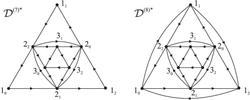
Figure 5: Graphs $\mathcal{D}^{(7)\ast}$, $\mathcal{D}^{(8)\ast}$

The unique cell system $W$ (up to equivalence) was computed in [21, Theorems 7.1, 7.3 & 7.4], and we use the same notation for the cells here. The $\mathcal{A}^{(n)\ast}$ graphs are illustrated in [21, Figure 11]. We illustrate the cases $n=7,8$ here in Figure 5. The numbering of the vertices of $\mathcal{A}^{(2m+1)\ast}$ that we use here is the same as that in [23], but the reverse of that used in [21]. The relations in $A(\mathcal{A}^{(n)\ast},W)$ are

$$W_{112}[121]+W_{111}[111]=0,$$

$$W_{p-1,p,p}[p(p-1)j]+W_{p,p,p}[ppp]+W_{p,p,p+1}[p(p+1)p]=0,$$ (16)

$$W_{p,p,p+1}[pp(p+1)]+W_{p,p+1,p+1}[p(p+1)(p+1)]=0,$$ (17)

$$W_{p,p,p+1}[(p+1)pp]+W_{p,p+1,p+1}[(p+1)(p+1)p]=0,$$ (18)

where $p=2,\ldots,r-1$ in (16), and $p=1,\ldots,p^{\prime}$ in (17), (18), where $r=\lfloor(n-1)/2\rfloor$, $p^{\prime}=r-1$ for even $n$, and $p^{\prime}=r-2$ for odd $n$. For even $n$ we have the extra relation $W_{r-1,r,r}[r(r-1)r]+W_{r,r,r}[rrr]=0$, and for odd $n$ we have the extra relation $[r(r-1)(r-1)]=[(r-1)(r-1)r]=0$.

We first consider the even case $n=2m+2$. Clearly all loops $[pp]$ of length 1 are in $A/[A,A]$, $p=1,\ldots,m$. Let $d_{l}^{p}:=\mathrm{dim}(pA_{l}p)$. From the Hilbert series for $A$, we see that $d_{2k}^{p}=d_{2k+1}^{p}=p=d_{2m-2k-1}^{p}=d_{2m-2k-2}^{p}$ if $p\leq k$ or $p\geq m-k+1$, and $d_{2k}^{p}=d_{2k+1}^{p}=k+1=d_{2m-2k-1}^{p}=d_{2m-2k-2}^{p}$ if $k+1\leq p\leq m-k$, for $2k\leq m-1$. Then $\mathrm{dim}(A^{S}_{2k})=\mathrm{dim}(A^{S}_{2k+1})=(k+1)(m-k)=\mathrm{dim}(A^{S}_{2m-2k-1})=\mathrm{dim}(A^{S}_{2m-2k-2})$ for $2k\leq m-1$.

Each commutator of the form $[[l(l+1)],[(l+1)l]]=[l(l+1)l]-[(l+1)l(l+1)]$ yields a relation between linearly independent paths of length 2 in $A/[A,A]$, $l=1,\ldots,m-1$. There are $m-1$ such relations, thus the dimension of $(A/[A,A])_{2}$ is $2(m-1)-(m-1)=m-1$. Similarly the dimension of $(A/[A,A])_{3}$ is $m-1$. Each commutator of the form $C_{p}=[[(p-1)ppp],[p(p-1)]]$, $p=2,\ldots,m$, and $C_{p}^{\prime}=[[(p-1)p(p+1)],[(p+1)p(p-1)]]$, $p=2,\ldots,m-1$, yield relations between linearly independent paths of length 4 in $A/[A,A]$. There is one basis path in $1A^{S}_{4}1$, which we may take to be $[11111]$. Let $w_{1}$ denote the basis element given by its image in $A/[A,A]$. Since $d_{4}^{2}=2$, the dimension of $2A^{S}_{4}2$ is 2. However, the basis can be chosen such that one of the basis paths is identified with $w_{1}$ in $A/[A,A]$ by $C_{2}$, thus we obtain one new basis path $w_{2}\in(A/[A,A])_{4}$, which may be chosen to be $[22222]$. Similarly, the dimension of $pA^{S}_{4}p$ is 3, $p=3,\ldots,m-2$, and the basis can be chosen such that two of the basis paths are identified with linear combinations of $w_{1},w_{2},\ldots,w_{p-1}$ in $A/[A,A]$ by $C_{p}$ and $C_{p}^{\prime}$. Thus we obtain one new basis path $w_{p}\in(A/[A,A])_{4}$ for each $p=3,\ldots,m-2$, which may be chosen to be $[ppppp]$. The dimension of $(m-1)A^{S}_{4}(m-1)$ is 2, but by $C_{m-1}$, $C_{m-1}^{\prime}$ any such path can be identified with a linear combination of $w_{1},w_{2},\ldots,w_{m-2}$ in $A/[A,A]$. Similarly the single basis path in $mA^{S}_{4}m$ can be identified with a linear combination of $w_{1},w_{2},\ldots,w_{m-2}$ in $A/[A,A]$. Thus we obtain a basis $\{w_{1},\ldots,w_{m-2}\}$ for $(A/[A,A])_{4}$. By a similar argument, we see that the dimension of $(A/[A,A])_{k}$ is $m-\lfloor k/2\rfloor$ for all $k=0,1,\ldots,2m-1$, with basis paths $[ppp\cdots p]$, for $p=1,\ldots,m-\lfloor k/2\rfloor$. Thus

$$HH_{0}(A)\cong S\oplus C,$$ (19)

where the graded vector space $C$ has Hilbert series $H_{C}(t)=\sum_{j=1}^{2m-1}(m-\lfloor j/2\rfloor)t^{j}$.

We now consider the odd case $n=2m+1$. Again, all loops $[pp]$ of length 1 are in $A/[A,A]$, this time for $p=1,\ldots,m-1$ (note that there is no edge from vertex $m$ to $m$ on $\mathcal{A}^{(2m+1)\ast}$). From the Hilbert series for $A$, we see that $d_{2k}$ is given by the same formula as for the even case $n=2m+2$, for $2k\leq m-1$, whilst $d_{2k+1}^{p}=p=d_{2m-2k-2}^{p}$ if $p\leq k$ or $p\geq m-k$, $d_{2k+1}^{p}=k+1=d_{2m-2k-3}^{p}$ if $k+1\leq i\leq m-k-1$, and $d_{2k+1}^{m}=0$, for $2k\leq m-2$. Then $\mathrm{dim}(A^{S}_{2k})=(k+1)(m-k)=\mathrm{dim}(A^{S}_{2m-2k-2})$ for $2k\leq m-1$, and $\mathrm{dim}(A^{S}_{2k-1})=(k+1)(m-k-1)=\mathrm{dim}(A^{S}_{2m-2k-3})$ for $2k\leq m-2$. By a similar argument as for the even case above, we see that the dimension of $(A/[A,A])_{k}$ is $m-\lfloor(k+1)/2\rfloor$ for all $k=0,1,\ldots,2m-2$, with basis paths $[ppp\cdots p]$, for $p=1,\ldots,m-\lfloor(k+1)/2\rfloor$. Thus

$$HH_{0}(A)\cong S\oplus C,$$ (20)

where the graded vector space $C$ has Hilbert series $H_{C}(t)=\sum_{j=1}^{2m-2}(m-\lfloor(j+1)/2\rfloor)t^{j}$.

3.3.4 The conjugate orbifold $\mathcal{D}^{\ast}$ graphs

The graphs $\mathcal{D}^{(n)\ast}$ are (three-colourable) unfolded versions, or $\mathbb{Z}_{3}$-orbifolds, of the graphs $\mathcal{A}^{(n)\ast}$, where we replace every vertex $v$ of $\mathcal{A}^{(n)\ast}$ by three vertices $v_{0}$, $v_{1}$, $v_{2}$, where $v_{a}$ is of colour $a$, such that there are edges $v_{0}\rightarrow w_{1}$, $v_{1}\rightarrow w_{2}$ and $v_{2}\rightarrow w_{0}$ if and only if there is an edge $v\rightarrow w$ on $\mathcal{A}^{(n)\ast}$. The graphs $\mathcal{D}^{(7)\ast}$, $\mathcal{D}^{(8)\ast}$ are illustrated in Figure 5.

Due to the three-colourability of the graph $\mathcal{D}^{(n)\ast}$, a closed loop on $\mathcal{A}^{(n)\ast}$ will only be a closed loop on $\mathcal{D}^{(n)\ast}$ if it has length $3k$, $k\geq 0$, and for each such closed loop on $\mathcal{A}^{(n)\ast}$, there are three corresponding closed loops of length $3k$ on $\mathcal{D}^{(n)\ast}$. However, these three closed loops are identified in $A/[A,A]$, which can be seen as follows. As in the case of $\mathcal{A}^{(n)\ast}$, $(A/[A,A])_{3k}$ is generated by paths of the form $[p_{l}p_{l+1}p_{l+2}p_{l}\cdots p_{l+3k}]$, for $l=0,1,2\textrm{ mod }3$ and $p=1,\ldots,r$, where $r=m-\lfloor 3k/2\rfloor$ for $n=2m+2$ and $r=m-\lfloor(3k+1)/2\rfloor$ for $n=2m+1$. Since $[p_{l}p_{l+1}p_{l+2}p_{l}\cdots p_{l}]$ is a cyclic permutation of $[p_{l+1}p_{l+2}p_{l}p_{l+1}\cdots p_{l+1}]$, we see that for $l=0,1,2\textrm{ mod }3$, the cyclic paths $[p_{l}p_{l+1}p_{l+2}p_{l}\cdots p_{l+3k}]$ are identified in $A/[A,A]$. Thus $(A/[A,A])_{3k}$ has a basis given by $[p_{0}p_{1}p_{2}p_{0}\cdots p_{0}]$, for $p=1,\ldots,r$, and $(A/[A,A])_{k^{\prime}}=0$ for $k^{\prime}\not\equiv 0\textrm{ mod }3$. Then

$$HH_{0}(A)\cong S\oplus C,$$ (21)

where for $n=2m+2$ the graded vector space $C$ has Hilbert series $H_{C}(t)=\sum_{j=1}^{\lfloor(2m-1)/3\rfloor}(m-\lfloor 3j/2\rfloor)t^{3j}$, whilst for $n=2m+1$, $H_{C}(t)=\sum_{j=1}^{\lfloor(2m-2)/3\rfloor}(m-\lfloor(3j+1)/2\rfloor)t^{3j}$.

3.3.5 The graph $\mathcal{E}^{(8)}$ for the conformal embedding $SU(3)_{5}\subset SU(6)_{1}$

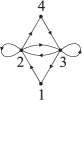
Figure 7: Graph $\mathcal{E}^{(8)\ast}$

We now consider the graph $\mathcal{E}^{(8)}$, illustrated in Figure 7. The unique cell system $W$ (up to equivalence) was computed in [21, Theorem 9.1]. The quotient algebra $A$ has the relations, for $l=0,1,2$,

$$[1_{l}2_{l+1}3_{l+2}]=[2_{l+1}3_{l+2}1_{l}]=[3_{l}2_{l+1}4_{l+2}]=[4_{l+2}3_{l}2_{l+1}]=0,$$

$$\sqrt{[3]}[2_{l}2_{l+1}2_{l+2}]=-[2_{l}3_{l+1}2_{l+2}],\qquad\sqrt{[3]}[3_{l}3_{l+1}3_{l+2}]=[3_{l}2_{l+1}3_{l+2}],$$

$$\frac{-\sqrt{[3]}}{[2]}[3_{l}1_{l+1}2_{l+2}]=[3_{l}2_{l+1}2_{l+2}]+[3_{l}3_{l+1}2_{l+2}],$$

$$\frac{-\sqrt{[3]}}{[2]}[2_{l}4_{l+1}3_{l+2}]=[2_{l}2_{l+1}3_{l+2}]+[2_{l}3_{l+1}3_{l+2}].$$

The only cyclic paths in $A_{+}$ are of the form $[2_{l}2_{l+1}2_{l+2}2_{l}]$, $[3_{l}3_{l+1}3_{l+2}3_{l}]$, $l=1,\ldots,3$. Now $[2_{l}2_{l+1}2_{l+2}2_{l}]=[2_{l+1}2_{l+2}2_{l}2_{l+1}]$ by cyclic permutation, and $\sqrt{[3]}[2_{l}2_{l+1}2_{l+2}2_{l}]=-[2_{l}3_{l+1}2_{l+2}2_{l}]=[3_{l+1}2_{l+2}2_{l}3_{l+1}]=-[3_{l+1}2_{l+2}3_{l}3_{l+1}]-(\sqrt{[2]}/\sqrt{[4]})[3_{l+1}2_{l+2}4_{l}3_{l+1}]=-\sqrt{[3]}[3_{l+1}3_{l+2}3_{l}3_{l+1}]$ in $A/[A,A]$, where the second and last equalities follows by cyclic permutation and the others follow from the relations in $A$. Thus we see that all cyclic paths in $A_{+}$ are identified in $A/[A,A]$ so that

$$HH_{0}(A)\cong S\oplus\mathbb{C}[2_{0}2_{1}2_{2}2_{0}].$$ (22)

3.3.6 The graph $\mathcal{E}^{(8)\ast}$ for the orbifold of the conformal embedding $SU(3)_{5}\subset SU(6)_{1}\rtimes\mathbb{Z}_{3}$

Consider the graph $\mathcal{E}^{(8)\ast}$, illustrated in Figure 7. The unique cell system $W$ (up to equivalence) was computed in [21, Theorem 10.1]. The quotient algebra $A$ has the relations

$$[123]=[231]=[324]=[432]=0,\qquad\qquad[222]=\frac{-1}{\sqrt{[3]}}[232],\qquad\qquad[333]=\frac{1}{\sqrt{[3]}}[323],$$

$$\frac{-\sqrt{[3]}}{[2]}[312]=[322]+[332],\qquad\qquad\frac{-\sqrt{[3]}}{[2]}[243]=[223]+[233].$$

Clearly the single edges $[22]$, $[33]$ are not in $[A,A]$, since the relations in $A$ only change paths of length $>1$, and edges are invariant under cyclic permutation. We have the relation $\sqrt{[3]}[222\cdots 2]=-[232\cdots 2]=-[322\cdots 23]$ for paths of length $r$ in $A/[A,A]$, $2\leq r\leq 5$, where the first equality follows from the relation in $A$ and the second follows by cyclic permutation. Thus in $A/[A,A]$, for $r=2$, we obtain $\sqrt{[3]}[222]=-[323]=-\sqrt{[3]}[333]$ by the relations in $A$. For $r=3$, we have $\sqrt{[3]}[2222]=-[3223]=[3323]+([2]/\sqrt{[3]})[3123]=\sqrt{[3]}[3333]$, by the relations in $A$, since the subpath $[123]=0$ in $A$. For $r=4$, we have $[3][22222]=-\sqrt{[3]}[32223]=[32323]=\sqrt{[3]}[33323]=[3][33333]$, by the relations in $A$, but also $\sqrt{[3]}[22222]=-[32223]=[33223]+([2]/\sqrt{[3]})[31223]=-[33233]-([2]/\sqrt{[3]})[33243]+([2]/\sqrt{[3]})[23122]=-\sqrt{[3]}[33333]$, by the relations in $A$, since the subpaths $[324]=0=[123]$ in $A$, and we have used the cyclic permutation relation in the penultimate equality. Then in $A/[A,A]$, we see that $[22222]=0=[33333]$. For $r=5$ we have $[3][222222]=-\sqrt{[3]}[322223]=[323223]=\sqrt{[3]}[333223]=-[3][333333]$ in $A/[A,A]$, by the relations in $A$. Thus

$$HH_{0}(A)\cong S\oplus C,$$ (23)

where the graded vector space $C=\mathbb{C}\{[22],[33]\}\oplus\mathbb{C}[222]\oplus\mathbb{C}[2222]\oplus\mathbb{C}[222222]$, and has Hilbert series $H_{C}(t)=2t+t^{2}+t^{3}+t^{5}$.

3.4 Determining the Hochschild homology of $A(\mathcal{G},W)$ for trivial Nakayama automorphism

In this section we determine the Hochschild and cyclic homology for the graphs $\mathcal{D}^{(3k)}$, $k\geq 2$, $\mathcal{A}^{(n)\ast}$, $n\geq 4$, $\mathcal{D}^{(3k)\ast}$, $k\geq 2$, and $\mathcal{E}^{(8)\ast}$. Here the almost Calabi-Yau algebra $A$ has trivial Nakayama automorphism.

In this case, the Hochschild homology of $A$ has minimal period at most 4, thus we have $HH_{i}(A)^{\ast}[h]\cong HH_{3-i}(A)$, $i=1,2$, and $HH_{i}(A)^{\ast}\cong HH_{7-i}(A)$, $i=3,4$. From the exactness of (12) we see that $\mathrm{ker}(B:\overline{HH}_{0}(A)\rightarrow\overline{HH}_{1}(A))=0$, and since the Connes differential $B$ preserves degrees, we have $\overline{HH}_{1}(A)\cong C\oplus X$, for some graded vector space $X$ which lives in degrees 1 to $h-2$. Then $\overline{HH}_{2}(A)\cong C^{\ast}[h]\oplus X^{\ast}[h]$, where $C\cong\overline{HH}_{0}(A)$ and $X^{\ast}[h]$ lives in degrees 2 to $h-1$. Now $B:\overline{HH}_{1}(A)\rightarrow\overline{HH}_{2}(A)$ restricts to an isomorphism $X\stackrel{{\scriptstyle\cong}}{{\longrightarrow}}X^{\ast}[h]$ since (12) is exact, and since it preserves degrees, $X$ only lives in degrees 2 to $h-2$. A similar argument shows that $\mathrm{ker}(B:\overline{HH}_{0}(A)\rightarrow\overline{HH}_{1}(A))\cong X^{\ast}[h]$, so that $\overline{HH}_{3}(A)\cong C^{\ast}[h]\oplus K^{\prime}$, where the graded vector space $K^{\prime}$ lives in degrees 3 to $h$, and $\overline{HH}_{4}(A)\cong C[h]\oplus K^{\prime\ast}[h]$, where $K^{\prime\ast}[h]$ lives in degrees $h$ to $2h-3$. Since $B:\overline{HH}_{3}(A)\rightarrow\overline{HH}_{4}(A)$ restricts to an isomorphism $K^{\prime}\stackrel{{\scriptstyle\cong}}{{\longrightarrow}}K^{\prime\ast}[h]$, we see that $K^{\prime}$ lives only in degree $h$. We will write $K^{\prime}=K[h]$ where $K$ is a vector space which lives in degree 0, so that $\overline{HH}_{3}(A)\cong C^{\ast}[h]\oplus K[h]$ and $\overline{HH}_{4}(A)\cong C[h]\oplus K^{\ast}[h]$.

Thus for any almost Calabi-Yau algebra $A$ with trivial Nakayama automorphism

$$\begin{array}[]{cccccccc}&&0&&&&&\\ (\textrm{min deg},\textrm{max deg})&&\downarrow&&&&&\\ (0,h-3)&&\overline{HH}_{0}(A)&\cong&C&&&\overline{HC}_{0}(A)\cong C\\ &&{\scriptstyle B}\downarrow&&{\scriptstyle\cong}\downarrow&&&\\ (1,h-2)&&\overline{HH}_{1}(A)&\cong&C&\oplus X&&\overline{HC}_{1}(A)\cong X\\ &&{\scriptstyle B}\downarrow&&&{\scriptstyle\cong}\downarrow&&\\ (2,h-1)&&\overline{HH}_{2}(A)&\cong&C^{\ast}[h]&\oplus X^{\ast}[h]&&\overline{HC}_{2}(A)\cong C^{\ast}[h]\\ &&{\scriptstyle B}\downarrow&&{\scriptstyle\cong}\downarrow&&&\\ (3,h)&&\overline{HH}_{3}(A)&\cong&C^{\ast}[h]&\oplus K[h]&&\overline{HC}_{3}(A)\cong K[h]\\ &&{\scriptstyle B}\downarrow&&&{\scriptstyle\cong}\downarrow&&\\ (h,2h-3)&&\overline{HH}_{4}(A)&\cong&C[h]&\oplus K^{\ast}[h]&&\overline{HC}_{4}(A)\cong C[h]\\ &&\downarrow&&&&&\\ &&\vdots&&&&&\\ \end{array}$$

where $X$ lives in degrees 2 to $h-2$, $K$ lives in degree 0, and $\overline{HH}_{5+i}(A)\cong\overline{HH}_{1+i}(A)[h]$, $\overline{HC}_{4+i}(A)\cong\overline{HC}_{i}(A)[h]$ for $i\geq 0$. Since $C$ is known, $X$ and $K$ can be determined from the Euler characteristic $\chi_{\overline{HC}(A)}(t)$ as they live in different degrees.

3.4.1 The graphs $\mathcal{D}^{(3k)}$

We consider the cases $\mathcal{D}^{(6k)}$, $\mathcal{D}^{(6k+3)}$ separately, $k\geq 1$. For the graph $\mathcal{D}^{(6k)}$, $k\geq 1$, $\mathrm{det}(H_{A}(t))=(1-t^{6k})^{4(3k(k-1)+2)/2}(1-t^{3k})/(1-t^{3})^{3}$, thus $\chi_{\overline{HC}(A)}(t)=(\sum_{j=1}^{2k-1}3t^{3j}-t^{3k}-(6k(k-1)+2)t^{6k})/(1-t^{6k})$. Then since $C$ has Hilbert series $H_{C}(t)=\sum_{j=1}^{2k-2}3t^{3j}+t^{6k-3}$, we see that $H_{X}(t)=t^{3}+\sum_{j=2}^{2k-2}3t^{3j}+t^{3k}+t^{6k-3}$ and $H_{K}(t)=6k(k-1)+2$, and we obtain:

Theorem 3.2

The Hochschild and cyclic homology of $A=A(\mathcal{D}^{(6k)},W)$, $k\geq 1$, where $W$ is equivalent to one of the cell systems constructed in [21], is given by

$$\begin{array}[]{lcl}HH_{0}(A)\cong S\oplus C,&&HC_{0}(A)\cong S\oplus C,\\ HH_{1}(A)\cong C\oplus X,&&HC_{1}(A)\cong X,\\ HH_{2}(A)\cong C^{\ast}[6k]\oplus X^{\ast}[6k],&&HC_{2}(A)\cong C^{\ast}[6k],\\ HH_{3}(A)\cong C^{\ast}[6k]\oplus K[6k],&&HC_{3}(A)\cong K[6k],\\ HH_{4}(A)\cong C[6k]\oplus K^{\ast}[6k],&&HC_{4}(A)\cong C[6k],\\ HH_{4+i}(A)\cong HH_{i}(A)[6k],\quad i\geq 1,&&HC_{4+i}(A)\cong HC_{i}(A)[6k],\quad i\geq 1,\end{array}$$

where the graded vector spaces $C$, $X$, $K$ have Hilbert series $H_{C}(t)=\sum_{j=1}^{2k-2}3t^{3j}+t^{6k-3}$, $H_{X}(t)=t^{3}+\sum_{j=2}^{2k-2}3t^{3j}+t^{3k}+t^{6k-3}$ and $H_{K}(t)=6k(k-1)+2$ respectively, where for $k=1$, $H_{X}(t)=0$.

For $\mathcal{D}^{(6k+3)}$, $k\geq 1$, $\mathrm{det}(H_{A}(t))=(1-t^{6k+3})^{6k^{2}+3}/(1-t^{3})^{3}$, thus $\chi_{\overline{HC}(A)}(t)=(\sum_{j=1}^{2k}3t^{3j}-6k^{2}t^{6k+3})/(1-t^{6k+3})$. Since $C$ has Hilbert series $H_{C}(t)=\sum_{j=1}^{2k-1}3t^{3j}+t^{6k}$, we see that $H_{X}(t)=t^{3}+\sum_{j=2}^{2k-1}3t^{3j}+t^{6k}$ and $H_{K}(t)=6k^{2}$, and we obtain:

Theorem 3.3

The Hochschild and cyclic homology of $A=A(\mathcal{D}^{(6k+3)},W)$, $k\geq 1$, where $W$ is equivalent to one of the cell systems constructed in [21], is given by

$$\begin{array}[]{lcl}HH_{0}(A)\cong S\oplus C,&&HC_{0}(A)\cong S\oplus C,\\ HH_{1}(A)\cong C\oplus X,&&HC_{1}(A)\cong X,\\ HH_{2}(A)\cong C^{\ast}[6k+3]\oplus X^{\ast}[6k+3],&&HC_{2}(A)\cong C^{\ast}[6k+3],\\ HH_{3}(A)\cong C^{\ast}[6k+3]\oplus K[6k+3],&&HC_{3}(A)\cong K[6k+3],\\ HH_{4}(A)\cong C[6k+3]\oplus K^{\ast}[6k+3],&&HC_{4}(A)\cong C[6k+3],\\ HH_{4+i}(A)\cong HH_{i}(A)[6k+3],\quad i\geq 1,&&HC_{4+i}(A)\cong HC_{i}(A)[6k+3],\quad i\geq 1,\end{array}$$

where the graded vector spaces $C$, $X$, $K$ have Hilbert series $H_{C}(t)=\sum_{j=1}^{2k-1}3t^{3j}+t^{6k}$, $H_{X}(t)=t^{3}+\sum_{j=2}^{2k-1}3t^{3j}+t^{6k}$ and $H_{K}(t)=6k^{2}$ respectively.

3.4.2 The $\mathcal{A}^{\ast}$ graphs

Let $D_{m}$, $D_{m}^{\prime}$ denote the determinant of the denominator $1-\Delta_{\mathcal{G}}t+\Delta_{\mathcal{G}}^{T}t^{2}-t^{3}$ of $H_{A}(t)$ for $\mathcal{G}=\mathcal{A}^{(2m+2)\ast},\mathcal{A}^{(2m+1)\ast}$ respectively, where $\Delta_{\mathcal{G}}$ denotes the adjacency matrix of $\mathcal{G}$, and let $T_{1}=1-t+t^{2}-t^{3}$, $T_{2}=t^{2}-t$. From the properties of determinants we can deduce the recursion relations $D_{m}=T_{1}D_{m-1}-T_{2}^{2}D_{m-2}$ and $D_{m}^{\prime}=(1-t^{3})D_{m-1}-T_{2}^{2}D_{m-2}$, for $m\geq 3$, and $D_{1}=T_{1}$, $D_{2}=T_{1}^{2}-T_{2}^{2}$. It is easy to show by induction on $m$ that $D_{m}=(1-t)^{m}(1-t^{2m+2})/(1-t^{2})$, and thus $D_{m}^{\prime}=(1-t)^{m-1}(1-t^{2m+1})$. Then for $\mathcal{A}^{(2m+2)\ast}$, $\mathrm{det}H_{A}(t)=(1-t^{2m+2})^{m}D_{m}^{-1}=(1-t^{2})(1-t^{2m+2})^{m-1}/(1-t)^{m}$, thus $\chi_{\overline{HC}(A)}(t)=(mt+(m-1)t^{2}+mt^{3}+(m-1)t^{4}+\cdots+(m-1)t^{2m}+mt^{2m+1})/(1-t^{2m+2})$. Then $H_{X}(t)=0=H_{K}(t)$, i.e. $X=0=K$. For $\mathcal{A}^{(2m+1)\ast}$, $\mathrm{det}H_{A}(t)=(1-t^{2m+1})^{m}(D_{m}^{\prime})^{-1}=(1-t^{2m+1})^{m-1}/(1-t)^{m-1}$, thus $\chi_{\overline{HC}(A)}(t)=((m-1)t+(m-1)t^{2}+(m-1)t^{3}+\cdots+(m-1)t^{2m})/(1-t^{2m+1})$. Then we again deduce that $H_{X}(t)=0=H_{K}(t)$, and we obtain:

Theorem 3.4

The Hochschild and cyclic homology of $A=A(\mathcal{A}^{(n)\ast},W)$, $n\geq 4$, where $W$ is any cell system on $\mathcal{A}^{(n)}$, is given by

$$\begin{array}[]{lcl}HH_{0}(A)\cong S\oplus C,&&HC_{0}(A)\cong S\oplus C,\\ HH_{1}(A)\cong C,&&HC_{1}(A)=0,\\ HH_{2}(A)\cong C^{\ast}[n],&&HC_{2}(A)\cong C^{\ast}[n],\\ HH_{3}(A)\cong C^{\ast}[n],&&HC_{3}(A)=0,\\ HH_{4}(A)\cong C[h],&&HC_{4}(A)\cong C[n],\\ HH_{4+i}(A)\cong HH_{i}(A)[n],\quad i\geq 1,&&HC_{4+i}(A)\cong HC_{i}(A)[n],\quad i\geq 1,\end{array}$$

where the graded vector space $C$ has Hilbert series $H_{C}(t)=\sum_{j=1}^{n-3}\lfloor(n-j-1)/2\rfloor t^{j}$.

3.4.3 The graph $\mathcal{D}^{(3k)\ast}$

The Nakayama automorphism is trivial for the graphs $\mathcal{D}^{(3k)\ast}$. We consider the cases $\mathcal{D}^{(6k)\ast}$, $\mathcal{D}^{(6k+3)\ast}$ separately. For the graph $\mathcal{D}^{(6k)\ast}$, $k\geq 1$, $\mathrm{det}(H_{A}(t))=(1-t^{6})(1-t^{6k})^{9k-6}/(1-t^{3})^{3k-1}$, thus $\chi_{\overline{HC}(A)}(t)=((3k-1)t^{3}+(3k-2)t^{6}+(3k-1)t^{9}+(3k-2)t^{12}+\cdots+(3k-1)t^{6k-3}-(6k-4)t^{6k})/(1-t^{6k})$. Then since $C$ has Hilbert series $H_{C}(t)=\sum_{j=1}^{\lfloor(2m-1)/3\rfloor}(m-\lfloor 3j/2\rfloor)t^{3j}$, we have $H_{X}(t)=0$, $H_{K}(t)=6k-4$, and we obtain:

Theorem 3.5

The Hochschild and cyclic homology of $A=A(\mathcal{D}^{(6k)\ast},W)$, $k\geq 1$, where $W$ is equivalent to one of the cell systems constructed in [21], is given by

$$\begin{array}[]{lcl}HH_{0}(A)\cong S\oplus C,&&HC_{0}(A)\cong S\oplus C,\\ HH_{1}(A)\cong C,&&HC_{1}(A)=0,\\ HH_{2}(A)\cong C^{\ast}[6k],&&HC_{2}(A)\cong C^{\ast}[6k],\\ HH_{3}(A)\cong C^{\ast}[6k]\oplus K[6k],&&HC_{3}(A)\cong K[6k],\\ HH_{4}(A)\cong C[6k]\oplus K^{\ast}[6k],&&HC_{4}(A)\cong C[6k],\\ HH_{4+i}(A)\cong HH_{i}(A)[6k],\quad i\geq 1,&&HC_{4+i}(A)\cong HC_{i}(A)[6k],\quad i\geq 1,\end{array}$$

where the graded vector spaces $C$, $K$ have Hilbert series $H_{C}(t)=\sum_{j=1}^{\lfloor(2m-1)/3\rfloor}(m-\lfloor 3j/2\rfloor)t^{3j}$ and $H_{K}(t)=6k-4$ respectively.

For $\mathcal{D}^{(6k+3)\ast}$, $k\geq 1$, $\mathrm{det}(H_{A}(t))=(1-t^{6k+3})^{9k}/(1-t^{3})^{3k}$, thus $\chi_{\overline{HC}(A)}(t)=(3kt^{3}+3kt^{6}+\cdots+3kt^{6k}-6kt^{6k+3})/(1-t^{6k+3})$. Since $C$ has Hilbert series $H_{C}(t)=\sum_{j=1}^{\lfloor(2m-2)/3\rfloor}(m-\lfloor(3j+1)/2\rfloor)t^{3j}$, we have $H_{X}(t)=0$, $H_{K}(t)=6k$, and we obtain:

Theorem 3.6

The Hochschild and cyclic homology of $A=A(\mathcal{D}^{(6k+3)\ast},W)$, $k\geq 1$, where $W$ is equivalent to one of the cell systems constructed in [21], is given by

$$\begin{array}[]{lcl}HH_{0}(A)\cong S\oplus C,&&HC_{0}(A)\cong S\oplus C,\\ HH_{1}(A)\cong C,&&HC_{1}(A)\cong X,\\ HH_{2}(A)\cong C^{\ast}[6k+3],&&HC_{2}(A)\cong C^{\ast}[6k+3],\\ HH_{3}(A)\cong C^{\ast}[6k+3]\oplus K[6k+3],&&HC_{3}(A)\cong K[6k+3],\\ HH_{4}(A)\cong C[6k+3]\oplus K^{\ast}[6k+3],&&HC_{4}(A)\cong C[6k+3],\\ HH_{4+i}(A)\cong HH_{i}(A)[6k+3],\quad i\geq 1,&&HC_{4+i}(A)\cong HC_{i}(A)[6k+3],\quad i\geq 1,\end{array}$$

where the graded vector spaces $C$, $K$ have Hilbert series $H_{C}(t)=\sum_{j=1}^{\lfloor(2m-2)/3\rfloor}(m-\lfloor(3j+1)/2\rfloor)t^{3j}$ and $H_{K}(t)=6k$ respectively.

3.4.4 The graph $\mathcal{E}^{(8)\ast}$

For the graph $\mathcal{E}^{(8)\ast}$, $\mathrm{det}(H_{A}(t))=(1-t^{2})(1-t^{4})(1-t^{8})^{2}/(1-t)^{2}$, thus $\chi_{\overline{HC}(A)}(t)=(2t+t^{2}+2t^{3}+2t^{5}+t^{6}+2t^{7}-2t^{8})/(1-t^{8})$. Then $H_{X}(t)=0$, $H_{K}(t)=2$, and we obtain:

Theorem 3.7

The Hochschild and cyclic homology of $A=A(\mathcal{E}^{(8)\ast},W)$, where $W$ is any cell system on $\mathcal{E}^{(8)\ast}$, is given by

$$\begin{array}[]{lcl}HH_{0}(A)\cong S\oplus C,&&HC_{0}(A)\cong S\oplus C,\\ HH_{1}(A)\cong C,&&HC_{1}(A)=0,\\ HH_{2}(A)\cong C^{\ast}[8],&&HC_{2}(A)\cong C^{\ast}[8],\\ HH_{3}(A)\cong C^{\ast}[8]\oplus K[8],&&HC_{3}(A)\cong K[8],\\ HH_{4}(A)\cong C[8]\oplus K^{\ast}[8],&&HC_{4}(A)\cong C[8],\\ HH_{4+i}(A)\cong HH_{i}(A)[8],\quad i\geq 1,&&HC_{4+i}(A)\cong HC_{i}(A)[8],\quad i\geq 1,\end{array}$$

where the graded vector spaces $C$, $K$ have Hilbert series $H_{C}(t)=2t+t^{2}+t^{3}+t^{5}$ and $H_{K}(t)=2$ respectively.

3.5 Determining the Hochschild homology of $A(\mathcal{G},W)$ for non-trivial Nakayama automorphism

We now determine the Hochschild and cyclic homology for the graphs $\mathcal{A}^{(n)}$, $n=4,5,6,7$, $\mathcal{E}^{(8)}$. Here the almost Calabi-Yau algebra $A$ has non-trivial Nakayama automorphism.

By a similar argument to that used in Section 3.4, for any almost Calabi-Yau algebra $A$ with non-trivial Nakayama automorphism, we have

$$\begin{array}[]{cccccccc}&&0&&&&&\\ (\textrm{min deg},\textrm{max deg})&&\downarrow&&&&&\\ (0,h-3)&&\overline{HH}_{0}(A)&\cong&C&&&\overline{HC}_{0}(A)\cong C\\ &&{\scriptstyle B}\downarrow&&{\scriptstyle\cong}\downarrow&&&\\ (1,h-2)&&\overline{HH}_{1}(A)&\cong&C&\oplus X_{1}&&\overline{HC}_{1}(A)\cong X_{1}\\ &&{\scriptstyle B}\downarrow&&&{\scriptstyle\cong}\downarrow&&\\ (2,h-1)&&\overline{HH}_{2}(A)&\cong&X_{2}&\oplus X_{1}&&\overline{HC}_{2}(A)\cong X_{2}\\ &&{\scriptstyle B}\downarrow&&{\scriptstyle\cong}\downarrow&&&\\ (3,h)&&\overline{HH}_{3}(A)&\cong&X_{2}&\oplus K_{1}[h]&&\overline{HC}_{3}(A)\cong K_{1}[h]\\ &&{\scriptstyle B}\downarrow&&&{\scriptstyle\cong}\downarrow&&\\ (h,2h-3)&&\overline{HH}_{4}(A)&\cong&X_{3}&\oplus K_{1}[h]&&\overline{HC}_{4}(A)\cong X_{3}\\ &&{\scriptstyle B}\downarrow&&{\scriptstyle\cong}\downarrow&&&\\ (h+1,2h-2)&&\overline{HH}_{5}(A)&\cong&X_{3}&\oplus X_{4}&&\overline{HC}_{5}(A)\cong X_{4}\\ &&{\scriptstyle B}\downarrow&&&{\scriptstyle\cong}\downarrow&&\\ (h+2,2h-1)&&\overline{HH}_{6}(A)&\cong&X_{3}^{\ast}[3h]&\oplus X_{4}^{\ast}[3h]&&\overline{HC}_{6}(A)\cong X_{3}^{\ast}[3h]\\ &&{\scriptstyle B}\downarrow&&{\scriptstyle\cong}\downarrow&&&\\ (h+3,2h)&&\overline{HH}_{7}(A)&\cong&X_{3}^{\ast}[3h]&\oplus K_{1}^{\ast}[2h]&&\overline{HC}_{7}(A)\cong K_{1}^{\ast}[2h]\\ &&{\scriptstyle B}\downarrow&&&{\scriptstyle\cong}\downarrow&&\\ (2h,3h-3)&&\overline{HH}_{8}(A)&\cong&X_{2}^{\ast}[3h]&\oplus K_{1}^{\ast}[2h]&&\overline{HC}_{8}(A)\cong X_{2}^{\ast}[3h]\\ &&{\scriptstyle B}\downarrow&&{\scriptstyle\cong}\downarrow&&&\\ (2h+1,3h-2)&&\overline{HH}_{9}(A)&\cong&X_{2}^{\ast}[3h]&\oplus X_{1}^{\ast}[3h]&&\overline{HC}_{9}(A)\cong X_{1}^{\ast}[3h]\\ &&{\scriptstyle B}\downarrow&&&{\scriptstyle\cong}\downarrow&&\\ (2h+2,3h-1)&&\overline{HH}_{10}(A)&\cong&C^{\ast}[3h]&\oplus X_{1}^{\ast}[3h]&&\overline{HC}_{10}(A)\cong C^{\ast}[3h]\\ &&{\scriptstyle B}\downarrow&&{\scriptstyle\cong}\downarrow&&&\\ (2h+3,3h)&&\overline{HH}_{11}(A)&\cong&C^{\ast}[3h]&\oplus K_{2}[3h]&&\overline{HC}_{11}(A)\cong K_{2}[3h]\\ &&{\scriptstyle B}\downarrow&&&{\scriptstyle\cong}\downarrow&&\\ (3h,4h-3)&&\overline{HH}_{12}(A)&\cong&C[3h]&\oplus K_{2}^{\ast}[3h]&&\overline{HC}_{12}(A)\cong C[3h]\\ &&\downarrow&&&&&\\ &&\vdots&&&&&\\ \end{array}$$

where $X_{1}$ lives in degrees 2 to $h-2$, $X_{2}$ lives in degrees 3 to $h-1$, $X_{3}$ lives in degrees $h+1$ to $2h-3$, $X_{4}$ lives in degrees $h+2$ to $2h-2$, $K_{i}$ lives in degree 0, $i=1,2$, and $\overline{HH}_{13+i}(A)\cong\overline{HH}_{1+i}(A)[3h]$, $\overline{HC}_{12+i}(A)\cong\overline{HC}_{i}(A)[3h]$ for $i\geq 0$. The graded vector space $K_{1}$ can be determined from the Euler characteristic $\chi_{\overline{HC}(A)}(t)$ as it is the only vector space which lives in degree $h$. The vector spaces $X_{1}$, $X_{3}$ can be determined by computing $\overline{HH}_{1}(A)$, $\overline{HH}_{4}(A)$ respectively. Then $X_{2}$, $X_{4}$, $K_{2}$ can each be determined from knowledge of $C\cong\overline{HH}_{0}(A)$, $X_{1}$, $X_{3}$ and the Euler characteristic.

3.5.1 The $\mathcal{A}$ graphs

Here we determine the Hochschild and cyclic homology for the graphs $\mathcal{A}^{(n)}$, $n=4,5,6,7$. The graphs $\mathcal{A}^{(n)}$, $n=5,6,7$, are illustrated in Figure 8. We have not yet been able to determine the Hochschild and cyclic homology for the case of general $n$.

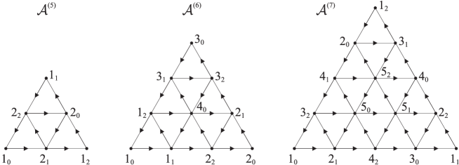
Figure 8: Graphs $\mathcal{A}^{(n)}$, $n=5,6,7$

We first consider the graph $\mathcal{A}^{(4)}$, for which $\mathrm{det}(H_{A}(t))=(1-t^{6})/(1-t^{3})$. Thus $\chi_{\overline{HC}(A)}(t)=(t^{3}+t^{6})/(1-t^{12})$ and we see that $H_{K_{1}}(t)=0$, and since $C=0$ for all the $\mathcal{A}$ graphs, $H_{K_{2}}(t)=0$. Since $\mathrm{ker}(\mu_{1}^{\prime})\subset(V\otimes_{S}A)^{S}=0$ and $\mathrm{ker}(\mu_{4}^{\prime})=\mathcal{N}^{S}=0$, we see that $\overline{HH}_{1}(A)=0=\overline{HH}_{4}(A)$. Thus $X_{1}=X_{3}=K_{1}=0$, and from $\chi_{\overline{HC}(A)}(t)$ we deduce that $X_{2}$ has Hilbert series $H_{X_{2}}(t)=t^{3}$ and $X_{4}=K_{2}=0$.

Theorem 3.8

The Hochschild and cyclic homology of $A=A(\mathcal{A}^{(4)},W)$, where $W$ is any cell system on $\mathcal{A}^{(4)}$, is given by

$$\begin{array}[]{lcl}HH_{0}(A)\cong S,&&HC_{0}(A)\cong S,\\ HH_{1}(A)=0,&&HC_{1}(A)=0,\\ HH_{2}(A)\cong X,&&HC_{2}(A)\cong X,\\ HH_{3}(A)\cong X,&&HC_{3}(A)=0,\\ HH_{4}(A)=0,&&HC_{4}(A)=0,\\ HH_{5}(A)=0,&&HC_{5}(A)=0,\\ HH_{6}(A)=0,&&HC_{6}(A)=0,\\ HH_{7}(A)=0,&&HC_{7}(A)=0,\\ HH_{8}(A)\cong X^{\ast}[12],&&HC_{8}(A)\cong X^{\ast}[12],\\ HH_{9}(A)\cong X^{\ast}[12],&&HC_{9}(A)=0,\\ HH_{10}(A)=0,&&HC_{10}(A)=0,\\ HH_{11}(A)=0,&&HC_{11}(A)=0,\\ HH_{12}(A)=0,&&HC_{12}(A)=0,\\ HH_{12+i}(A)\cong HH_{i}(A)[12],\quad i\geq 1,&&HC_{12+i}(A)\cong HC_{i}(A)[12],\quad i\geq 1,\end{array}$$

where the graded vector space $X$ has Hilbert series $H_{X}(t)=t^{3}$.

We now consider the graph $\mathcal{A}^{(5)}$, for which $\mathrm{det}(H_{A}(t))=(1-t^{15})/(1-t^{3})$. Thus $\chi_{\overline{HC}(A)}(t)=(t^{3}+t^{6}+t^{9}+t^{12})/(1-t^{15})$ and we see that $H_{K_{1}}(t)=0$, and since $C=0$ for all the $\mathcal{A}$ graphs, $H_{K_{2}}(t)=0$. We now explicitly determine $\overline{HH}_{1}(A)$ and $\overline{HH}_{4}(A)$.

We begin with the graded vector space $Y=\overline{HH}_{1}(A)=\mathrm{ker}(\mu_{1}^{\prime})/\mathrm{Im}(\mu_{2}^{\prime})$, and consider each graded piece $Y_{j}$ separately. Due to the three-colourability of $\mathcal{A}^{(5)}$, $Y_{j}=0$ for $j=1,2$. Thus we only need to determine $Y_{3}$. A basis for $(\widetilde{V}\otimes_{S}A)^{S}_{2}$ is given by the elements $[2_{l+1}1_{l}]\otimes[1_{l}2_{l+1}]$, $[1_{l+1}2_{l}]\otimes[2_{l}1_{l+1}]$ and $[2_{l+1}2_{l}]\otimes[2_{l}2_{l+1}]$, for $l=0,1,2\textrm{ mod }3$. We have $\mu_{2}^{\prime}([2_{l+1}1_{l}]\otimes[1_{l}2_{l+1}])=W_{1_{l}2_{l+1}2_{l+2}}([2_{l+1}2_{l+2}]\otimes[2_{l+2}1_{l}2_{l+1}]+[1_{l}2_{l+1}]\otimes[2_{l+1}2_{l+2}1_{l}])=W_{2_{l}2_{l+1}2_{l+2}}[2_{l+1}2_{l+2}]\otimes[2_{l+2}2_{l}2_{l+1}]$, using the relations in $A$. Thus we see that $[2_{l+1}2_{l+2}]\otimes[2_{l+2}2_{l}2_{l+1}]=0$ in $Y_{3}$, $l=0,1,2\textrm{ mod }3$. Thus $Y_{3}=0$ and we obtain $\overline{HH}_{1}(A)=0$. Since $X_{1}=0$, we deduce from $\chi_{\overline{HC}(A)}(t)$ that $X_{2}$ has Hilbert series $H_{X_{2}}(t)=t^{3}$.

We now consider $Y^{\prime}=\overline{HH}_{4}(A)$, which lives in degrees 5 to 7. Now $\mathrm{ker}(\mu_{4}^{\prime})=\mathcal{N}^{S}[5]$, since $\sum_{j}w_{j}^{\ast}\beta(x)w_{j}=0$ for all $x\in\mathcal{N}^{S}_{+}$ and $\mathcal{N}^{S}_{0}=0$. As with $\overline{HH}_{1}(A)$, $Y^{\prime}_{j}=0$ for $j=5,7$, due to the three-colourability of $\mathcal{A}^{(5)}$. We now determine $Y^{\prime}_{6}$. A basis for $(V\otimes_{S}\mathcal{N})^{S}_{1}$ is given by $[2_{l}2_{l+1}]\otimes[2_{l+1}]$, $l=0,1,2\textrm{ mod }3$, and a basis for $\mathcal{N}^{S}$ is given by $[2_{l}2_{l+1}]$, $l=0,1,2\textrm{ mod }3$. Now $\mu_{5}^{\prime}([2_{l}2_{l+1}]\otimes[2_{l+1}])=[2_{l+1}2_{l+2}]-[2_{l}2_{l+1}]$, thus $[2_{0}2_{1}]=[2_{1}2_{2}]=[2_{2}2_{0}]$ in $Y^{\prime}_{6}$. Then $\overline{HH}_{4}(A)=\mathbb{C}[2_{0}2_{1}][5]=X_{3}$, and we deduce from $\chi_{\overline{HC}(A)}(t)$ that $X_{4}=0$.

Theorem 3.9

The Hochschild and cyclic homology of $A=A(\mathcal{A}^{(5)},W)$, where $W$ is any cell system on $\mathcal{A}^{(5)}$, is given by

$$\begin{array}[]{lcl}HH_{0}(A)\cong S,&&HC_{0}(A)\cong S,\\ HH_{1}(A)=0,&&HC_{1}(A)=0,\\ HH_{2}(A)\cong X_{2},&&HC_{2}(A)\cong X_{2},\\ HH_{3}(A)\cong X_{2},&&HC_{3}(A)=0,\\ HH_{4}(A)\cong X_{3},&&HC_{4}(A)\cong X_{3},\\ HH_{5}(A)\cong X_{3},&&HC_{5}(A)=0,\\ HH_{6}(A)\cong X_{3}^{\ast}[15],&&HC_{6}(A)\cong X_{3}^{\ast}[15],\\ HH_{7}(A)\cong X_{3}^{\ast}[15],&&HC_{7}(A)=0,\\ HH_{8}(A)\cong X_{2}^{\ast}[15],&&HC_{8}(A)\cong X_{2}^{\ast}[15],\\ HH_{9}(A)\cong X_{2}^{\ast}[15],&&HC_{9}(A)=0,\\ HH_{10}(A)=0,&&HC_{10}(A)=0,\\ HH_{11}(A)=0,&&HC_{11}(A)=0,\\ HH_{12}(A)=0,&&HC_{12}(A)=0,\\ HH_{12+i}(A)\cong HH_{i}(A)[15],\quad i\geq 1,&&HC_{12+i}(A)\cong HC_{i}(A)[15],\quad i\geq 1,\end{array}$$

where the graded vector spaces $X_{2}$ and $X_{3}$ have Hilbert series $H_{X_{2}}(t)=t^{3}$ and $H_{X_{3}}(t)=t^{6}$.

We now consider the graph $\mathcal{A}^{(6)}$, for which $\mathrm{det}(H_{A}(t))=(1-t^{6})(1-t^{9})(1-t^{18})/(1-t^{3})$. Thus $\chi_{\overline{HC}(A)}(t)=(t^{3}+t^{15}-2t^{18})/(1-t^{18})$ and we see that $H_{K_{1}}(t)=0$, and since $C=0$ for all the $\mathcal{A}$ graphs, $H_{K_{2}}(t)=2$. We now explicitly determine $\overline{HH}_{1}(A)$ and $\overline{HH}_{4}(A)$.

We begin with the graded vector space $Y=\overline{HH}_{1}(A)$. Due to the three-colourability of $\mathcal{A}^{(6)}$, $Y_{j}=0$ for $j=1,2,4$, so we only need to determine $Y_{3}$. A basis for $(\widetilde{V}\otimes_{S}A)^{S}_{2}$ is given by the elements $[i_{l+1}i_{l}]\otimes[i_{l}i_{l+1}]$, $[(i+1)_{2}i_{1}]\otimes[i_{1}(i+1)_{2}]$, $[i_{1}4_{0}]\otimes[4_{0}i_{1}]$, and $[4_{0}i_{2}]\otimes[i_{2}4_{0}]$, for $l=0,1,2$, $i=1,2,3\textrm{ mod }3$. A basis for $(V\otimes A)^{S}_{3}$ is given by $[4_{0}i_{1}]\otimes[i_{1}i_{2}4_{0}]$, $[i_{1}i_{2}]\otimes[i_{2}4_{0}i_{1}]$ and $[i_{2}4_{0}]\otimes[4_{0}i_{1}i_{2}]$, for $i=1,2,3\textrm{ mod }3$. Under $\mu_{2}^{\prime}$ the basis elements of $(\widetilde{V}\otimes_{S}A)^{S}_{2}$ yield the following expressions after using the relations in $A$, for $i=1,2,3\textrm{ mod }3$:

$$\mu_{2}^{\prime}([i_{1}i_{0}]\otimes[i_{0}i_{1}])=-W_{4_{0}i_{1}i_{2}}[i_{1}i_{2}]\otimes[i_{2}4_{0}i_{1}]=\mu_{2}^{\prime}([i_{0}i_{2}]\otimes[i_{2}i_{0}]),$$

$$\mu_{2}^{\prime}([i_{2}i_{1}]\otimes[i_{1}i_{2}])=W_{4_{0}i_{1}i_{2}}[4_{0}i_{1}]\otimes[i_{1}i_{2}4_{0}]+W_{4_{0}i_{1}i_{2}}[i_{2}4_{0}]\otimes[4_{0}i_{1}i_{2}],$$

$$\mu_{2}^{\prime}([(i+1)_{2}i_{1}]\otimes[i_{1}(i+1)_{2}])=W_{4_{0}i_{1}(i+1)_{2}}[4_{0}i_{1}]\otimes[i_{1}(i+1)_{2}4_{0}]$$

$$\qquad\qquad\qquad\qquad\qquad\qquad\qquad+W_{4_{0}i_{1}(i+1)_{2}}[(i+1)_{2}4_{0}]\otimes[4_{0}i_{1}(i+1)_{2}],$$

$$\mu_{2}^{\prime}([i_{1}4_{0}]\otimes[4_{0}i_{1}])=W_{4_{0}i_{1}i_{2}}[i_{2}4_{0}]\otimes[4_{0}i_{1}i_{2}]+W_{4_{0}i_{1}(i+1)_{2}}[(i+1)_{2}4_{0}]\otimes[4_{0}i_{1}(i+1)_{2}]$$

$$\qquad\qquad\qquad\qquad\qquad+W_{4_{0}i_{1}i_{2}}[i_{1}i_{2}]\otimes[i_{2}4_{0}i_{1}],$$

$$\mu_{2}^{\prime}([4_{0}i_{2}]\otimes[i_{2}4_{0}])=W_{4_{0}i_{1}i_{2}}[4_{0}i_{1}]\otimes[i_{1}i_{2}4_{0}]+W_{4_{0}(i-1)_{1}i_{2}}[4_{0}(i-1)_{1}]\otimes[(i-1)_{1}i_{2}4_{0}]$$

$$\qquad\qquad\qquad\qquad\qquad+W_{4_{0}i_{1}i_{2}}[i_{1}i_{2}]\otimes[i_{2}4_{0}i_{1}].$$

Then from $\mathrm{Im}(\mu_{2}^{\prime})_{3}$ we obtain the following relations in $Y_{3}$: $[i_{1}i_{2}]\otimes[i_{2}4_{0}i_{1}]=0$ and $[4_{0}i_{1}]\otimes[i_{1}i_{2}4_{0}]=-[i_{2}4_{0}]\otimes[4_{0}i_{1}i_{2}]=(W_{4_{0}3_{1}3_{2}}/W_{4_{0}i_{1}i_{2}})[4_{0}3_{1}]\otimes[3_{1}1_{2}4_{0}]$.

We now consider $\mathrm{Ker}(\mu_{1}^{\prime})_{3}$. Let $x=\sum_{i=1}^{3}(\lambda_{i}^{0}[i_{2}4_{0}]\otimes[4_{0}i_{1}i_{2}]+\lambda_{i}^{1}[4_{0}i_{1}]\otimes[i_{1}i_{2}4_{0}]+\lambda_{i}^{2}[i_{1}i_{2}]\otimes[i_{2}4_{0}i_{1}])$ be a general element in $(V\otimes A)^{S}_{3}$. Since $\mu_{1}^{\prime}(x)=\sum_{i=1}^{3}((\lambda_{i}^{0}-\lambda_{i}^{1})[4_{0}i_{1}i_{2}4_{0}]+(\lambda_{i}^{1}-\lambda_{i}^{2})[i_{1}i_{2}4_{0}i_{1}]+(\lambda_{i}^{2}-\lambda_{i}^{0})[i_{2}4_{0}i_{1}i_{2}])$, then $x\in\mathrm{Ker}(\mu_{1}^{\prime})$ if and only if $\lambda_{i}^{0}=\lambda_{i}^{1}=\lambda_{i}^{2}$ for each $i=1,2,3$. Using the relations from $\mathrm{Im}(\mu_{2}^{\prime})_{3}$, a general element in $Y_{3}$ is thus of the form $\sum_{i}\lambda_{i}^{0}([i_{2}4_{0}]\otimes[4_{0}i_{1}i_{2}]+[4_{0}i_{1}]\otimes[i_{1}i_{2}4_{0}]+[i_{1}i_{2}]\otimes[i_{2}4_{0}i_{1}])=\sum_{i}\lambda_{i}^{0}(-(W_{4_{0}3_{1}3_{2}}/W_{4_{0}i_{1}i_{2}})[4_{0}3_{1}]\otimes[3_{1}1_{2}4_{0}]+0+(W_{4_{0}3_{1}3_{2}}/W_{4_{0}i_{1}i_{2}})[4_{0}3_{1}]\otimes[3_{1}1_{2}4_{0}])=0$. Thus $Y_{3}=0$ and we obtain $\overline{HH}_{1}(A)=0$. Since $X_{1}=0$, we deduce from $\chi_{\overline{HC}(A)}(t)$ that $X_{2}$ is a graded vector space with Hilbert series $H_{X_{2}}(t)=t^{3}$.

We now consider $Y^{\prime}=\overline{HH}_{4}(A)$, which lives in degrees 6 to 9. Now $\mathcal{N}^{S}_{0}=\mathbb{C}[4_{0}]$, but $\mu_{4}^{\prime}(\lambda[4_{0}])=2\lambda[4_{0}1_{1}1_{2}4_{0}]$, thus $\lambda[4_{0}]\in\mathrm{ker}(\mu_{4}^{\prime})$ if and only if $\lambda=0$. Thus $\mathrm{ker}(\mu_{4}^{\prime})=\mathcal{N}^{S}_{+}[6]$, since $\sum_{j}w_{j}^{\ast}\beta(x)w_{j}=0$ for all $x\in\mathcal{N}^{S}_{+}=\mathbb{C}[4_{0}1_{1}1_{2}4_{0}]$. As with $\overline{HH}_{1}(A)$, $Y^{\prime}_{j}=0$ for $j=7,8$, due to the three-colourability of $\mathcal{A}^{(6)}$, and $Y^{\prime}_{6}=0$ since $\mathrm{ker}(\mu_{4}^{\prime})_{6}=0$. We now determine $Y^{\prime}_{9}$. A basis for $(V\otimes_{S}\mathcal{N})^{S}_{1}$ is given by $[4_{0}i_{1}]\otimes[i_{1}i_{2}4_{0}]$, $[i_{1}(i+1)_{2}]\otimes[(i+1)_{2}4_{0}(i-1)_{1}]$ and $[i_{2}4_{0}]\otimes[4_{0}(i-1)_{1}(i-1)_{2}]$, $i=0,1,2\textrm{ mod }3$. Now $\mu_{5}^{\prime}([4_{0}1_{1}]\otimes[1_{1}1_{2}4_{0}])=-[4_{0}1_{1}1_{2}4_{0}]$, thus $\mathrm{Im}(\mu_{5}^{\prime})=\mathcal{N}^{S}_{+}$. Then $Y^{\prime}_{9}=0$ and we obtain $\overline{HH}_{4}(A)=0$. Then since $X_{3}=0$, we deduce from $\chi_{\overline{HC}(A)}(t)$ that $X_{4}=0$.

Theorem 3.10

The Hochschild and cyclic homology of $A=A(\mathcal{A}^{(6)},W)$, where $W$ is any cell system on $\mathcal{A}^{(6)}$, is given by

$$\begin{array}[]{lcl}HH_{0}(A)\cong S,&&HC_{0}(A)\cong S,\\ HH_{1}(A)=0,&&HC_{1}(A)=0,\\ HH_{2}(A)\cong X,&&HC_{2}(A)\cong X,\\ HH_{3}(A)\cong X,&&HC_{3}(A)=0,\\ HH_{4}(A)=0,&&HC_{4}(A)=0,\\ HH_{5}(A)=0,&&HC_{5}(A)=0,\\ HH_{6}(A)=0,&&HC_{6}(A)=0,\\ HH_{7}(A)=0,&&HC_{7}(A)=0,\\ HH_{8}(A)\cong X^{\ast}[18],&&HC_{8}(A)\cong X^{\ast}[18],\\ HH_{9}(A)\cong X^{\ast}[18],&&HC_{9}(A)=0,\\ HH_{10}(A)=0,&&HC_{10}(A)=0,\\ HH_{11}(A)\cong K[18],&&HC_{11}(A)\cong K[18],\\ HH_{12}(A)\cong K^{\ast}[18],&&HC_{12}(A)=0,\\ HH_{12+i}(A)\cong HH_{i}(A)[18],\quad i\geq 1,&&HC_{12+i}(A)\cong HC_{i}(A)[18],\quad i\geq 1,\end{array}$$

where the graded vector spaces $X$ and $K$ have Hilbert series $H_{X}(t)=t^{3}$ and $H_{K}(t)=2$.

We now consider the graph $\mathcal{A}^{(7)}$, for which $\mathrm{det}(H_{A}(t))=(1-t^{21})^{3}/(1-t^{3})$. Thus $\chi_{\overline{HC}(A)}(t)=(t^{3}+t^{6}+\cdots+t^{18}-2t^{21})/(1-t^{21})$ and we see that $H_{K_{1}}(t)=0$, and since $C=0$ for all the $\mathcal{A}$ graphs, $H_{K_{2}}(t)=2$. We now explicitly determine $\overline{HH}_{1}(A)$ and $\overline{HH}_{4}(A)$.

We begin with the graded vector space $Y=\overline{HH}_{1}(A)$. Due to the three-colourability of $\mathcal{A}^{(7)}$, $Y_{j}=0$ for $j=1,2,4,5$, so we only need to determine $Y_{3}$. A basis for $(\widetilde{V}\otimes_{S}A)^{S}_{2}$ is given by the elements $[1_{l}3_{l-1}]\otimes[3_{l-1}1_{l}]$, $[2_{l}1_{l-1}]\otimes[1_{l-1}2_{l}]$, $[2_{l}5_{l-1}]\otimes[5_{l-1}2_{l}]$, $[3_{l}2_{l-1}]\otimes[2_{l-1}3_{l}]$, $[3_{l}4_{l-1}]\otimes[4_{l-1}3_{l}]$, $[4_{l}2_{l-1}]\otimes[2_{l-1}4_{l}]$, $[4_{l}5_{l-1}]\otimes[5_{l-1}4_{l}]$, $[5_{l}3_{l-1}]\otimes[3_{l-1}5_{l}]$, $[5_{l}4_{l-1}]\otimes[4_{l-1}5_{l}]$ and $[5_{l}5_{l-1}]\otimes[5_{l-1}5_{l}]$, for $l=0,1,2\textrm{ mod }3$. A basis for $(V\otimes A)^{S}_{3}$ is given by $[2_{l}3_{l+1}]\otimes[3_{l+1}5_{l+2}2_{l}]$, $[3_{l}5_{l+1}]\otimes[5_{l+1}2_{l+2}3_{l}]$, $[4_{l}5_{l+1}]\otimes[5_{l+1}2_{l+2}4_{l}]$, $[5_{l}2_{l+1}]\otimes[2_{l+1}3_{l+2}5_{l}]$, $[5_{l}4_{l+1}]\otimes[4_{l+1}3_{l+2}5_{l}]$ and $[5_{l}5_{l+1}]\otimes[5_{l+1}4_{l+2}5_{l}]$, for $l=0,1,2\textrm{ mod }3$. Under $\mu_{2}^{\prime}$ the basis elements of $(\widetilde{V}\otimes_{S}A)^{S}_{2}$ yield the following expressions after using the relations in $A$, for $l=0,1,2\textrm{ mod }3$:

$$\mu_{2}^{\prime}([1_{l}3_{l-1}]\otimes[3_{l-1}1_{l}]) = W_{235}[2_{l+1}3_{l-1}]\otimes[3_{l-1}5_{l}2_{l+1}]\;\;=\;\;\mu_{2}^{\prime}([2_{l+1}1_{l}]\otimes[1_{l}2_{l+1}]),$$

$$\mu_{2}^{\prime}([2_{l}5_{l-1}]\otimes[5_{l-1}2_{l}]) = W_{235}[3_{l+1}5_{l-1}]\otimes[5_{l-1}2_{l}3_{l+1}]+W_{245}[4_{l+1}5_{l-1}]\otimes[5_{l-1}2_{l}4_{l+1}]$$

$$\quad+W_{235}[2_{l+1}3_{l-1}]\otimes[3_{l-1}5_{l}2_{l+1}],$$

$$\mu_{2}^{\prime}([3_{l}2_{l-1}]\otimes[2_{l-1}3_{l}]) = W_{235}[5_{l+1}2_{l-1}]\otimes[2_{l-1}3_{l}5_{l+1}]+W_{235}[3_{l}5_{l+1}]\otimes[5_{l+1}2_{l-1}3_{l}],$$

$$\mu_{2}^{\prime}([3_{l}4_{l-1}]\otimes[4_{l-1}3_{l}]) = W_{354}[5_{l+1}4_{l-1}]\otimes[4_{l-1}3_{l}5_{l+1}]-W_{235}[3_{l}5_{l+1}]\otimes[5_{l+1}2_{l-1}3_{l}],$$

$$\mu_{2}^{\prime}([4_{l}2_{l-1}]\otimes[2_{l-1}4_{l}]) = -W_{235}[5_{l+1}2_{l-1}]\otimes[2_{l-1}3_{l}5_{l+1}]+W_{245}[4_{l}5_{l+1}]\otimes[5_{l+1}2_{l-1}4_{l}],$$

$$\mu_{2}^{\prime}([4_{l}5_{l-1}]\otimes[5_{l-1}4_{l}]) = W_{455}[5_{l+1}5_{l-1}]\otimes[5_{l-1}4_{l}5_{l+1}]-W_{245}[4_{l}5_{l+1}]\otimes[5_{l+1}2_{l-1}4_{l}]$$

$$\quad-W_{235}[3_{l+1}5_{l-1}]\otimes[5_{l-1}2_{l}3_{l+1}],$$

$$\mu_{2}^{\prime}([5_{l}3_{l-1}]\otimes[3_{l-1}5_{l}]) = W_{354}[5_{l}4_{l+1}]\otimes[4_{l+1}3_{l-1}5_{l}]+W_{235}[5_{l}2_{l+1}]\otimes[2_{l+1}3_{l-1}5_{l}]$$

$$\quad+W_{235}[2_{l+1}3_{l-1}]\otimes[3_{l-1}5_{l}2_{l+1}],$$

$$\mu_{2}^{\prime}([5_{l}4_{l-1}]\otimes[4_{l-1}5_{l}]) = -W_{354}[5_{l+1}4_{l-1}]\otimes[4_{l-1}3_{l}5_{l+1}]+W_{455}[5_{l}5_{l+1}]\otimes[5_{l+1}4_{l-1}5_{l}]$$

$$\quad-W_{235}[5_{l}2_{l+1}]\otimes[2_{l}3_{l-1}5_{l}],$$

$$\mu_{2}^{\prime}([5_{l}5_{l-1}]\otimes[5_{l-1}5_{l}]) = -W_{245}[4_{l+1}5_{l-1}]\otimes[5_{l-1}2_{l}4_{l+1}]-W_{354}[5_{l}4_{l+1}]\otimes[4_{l+1}3_{l-1}5_{l}]$$

$$\quad-W_{455}[5_{l+1}5_{l-1}]\otimes[5_{l-1}4_{l}5_{l+1}]-W_{455}[5_{l}5_{l+1}]\otimes[5_{l+1}4_{l-1}5_{l}],$$

where $W_{ijk}:=W_{i_{0}j_{1}k_{2}}=W_{i_{1}j_{2}k_{0}}=W_{i_{2}j_{0}k_{1}}$ for vertices $i_{l}$, $j_{l}$, $k_{l}$ of $\mathcal{A}^{(7)}$, $l=0,1,2$. Then from $\mathrm{Im}(\mu_{2}^{\prime})_{3}$ we obtain the following relations in $Y_{3}$:

$$\begin{array}[]{l}{}[2_{l}3_{l+1}]\otimes[3_{l+1}5_{l+2}2_{l}]=0,\quad l=0,1,2\textrm{ mod }3,\qquad\qquad[5_{0}5_{1}]\otimes[5_{1}4_{2}5_{0}]=-x_{2}-x_{3},\\ {}[3_{0}5_{1}]\otimes[5_{1}2_{2}3_{0}]=-(W_{245}/W_{235})[4_{0}5_{1}]\otimes[5_{1}2_{2}4_{0}]=-[5_{1}2_{2}]\otimes[2_{2}3_{0}5_{1}]\\ \hskip 83.93562pt=(W_{354}/W_{235})[5_{1}4_{2}]\otimes[4_{2}3_{0}5_{1}]=(W_{354}/W_{235})x_{1}-(W_{455}/W_{235})x_{2},\\ {}[3_{1}5_{2}]\otimes[5_{2}2_{0}3_{1}]=-(W_{245}/W_{235})[4_{1}5_{2}]\otimes[5_{2}2_{0}4_{1}]=-[5_{2}2_{0}]\otimes[2_{0}3_{1}5_{2}]=(W_{354}/W_{235})x_{1},\\ {}[3_{2}5_{0}]\otimes[5_{0}2_{1}3_{2}]=-(W_{245}/W_{235})[4_{2}5_{0}]\otimes[5_{0}2_{1}4_{2}]=-[5_{0}2_{1}]\otimes[2_{1}3_{2}5_{0}]\\ \hskip 83.93562pt=(W_{354}/W_{235})[5_{0}4_{1}]\otimes[4_{1}3_{2}5_{0}]=(W_{354}/W_{235})x_{1}+(W_{455}/W_{235})x_{3},\end{array}$$

where $x_{1}=[5_{2}4_{0}]\otimes[4_{0}3_{1}5_{2}]$, $x_{2}=[5_{1}5_{2}]\otimes[5_{2}4_{0}5_{1}]$ and $x_{3}=[5_{2}5_{0}]\otimes[5_{0}4_{1}5_{2}]$.

We now consider $\mathrm{Ker}(\mu_{1}^{\prime})_{3}$. Let $x=\sum_{l=0}^{2}(\lambda_{1}^{l}[3_{l}5_{l+1}]\otimes[5_{l+1}2_{l+2}3_{l}]+\lambda_{2}^{l}[4_{l}5_{l+1}]\otimes[5_{l+1}2_{l+2}4_{l}]+\lambda_{3}^{l}[5_{l}2_{l+1}]\otimes[2_{l+1}3_{l+2}5_{l}]+\lambda_{4}^{l}[5_{l}4_{l+1}]\otimes[4_{l+1}3_{l+2}5_{l}]+\lambda_{5}^{l}[5_{l}5_{l+1}]\otimes[5_{l+1}4_{l+2}5_{l}])$ be a general element in $(V\otimes A)^{S}_{3}$. Now $\mu_{1}^{\prime}(x)=\sum_{l=0}^{2}(\lambda_{3}^{l-1}[2_{l}3_{l+1}5_{l+2}2_{l}]-\lambda_{1}^{l}[3_{l}5_{l+1}2_{l+2}3_{l}]+(\lambda_{1}^{l-1}-\lambda_{2}^{l-1}(W_{235}/W_{245})-\lambda_{3}^{l}+\lambda_{4}^{l}(W_{235}/W_{354})+(\lambda_{5}^{l-1}-\lambda_{5}^{l})(W_{235}/W_{455}))[5_{l}2_{l+1}3_{l+2}5_{l}])=0$ if and only if $\lambda_{1}^{l}=\lambda_{3}^{l}=0,\lambda_{4}^{l}=\lambda_{2}^{l-1}+(\lambda_{5}^{l}-\lambda_{5}^{l-1})(W_{354}/W_{455})$, for $l=0,1,2\textrm{ mod }3$. Using the relations from $\mathrm{Im}(\mu_{2}^{\prime})_{3}$, a general element in $Y_{3}$ is thus of the form $\sum_{l=0}^{2}(\lambda_{2}^{l}[4_{l}5_{l+1}]\otimes[5_{l+1}2_{l+2}4_{l}]+(\lambda_{2}^{l-1}+(\lambda_{5}^{l}-\lambda_{5}^{l-1})(W_{354}/W_{455}))[5_{l}4_{l+1}]\otimes[4_{l+1}3_{l+2}5_{l}]+\lambda_{5}^{l}[5_{l}5_{l+1}]\otimes[5_{l+1}4_{l+2}5_{l}])=0$. Thus $Y_{3}=0$ and we obtain $\overline{HH}_{1}(A)=0$. Since $X_{1}=0$, we deduce from $\chi_{\overline{HC}(A)}(t)$ that $X_{2}$ is a graded vector space with Hilbert series $H_{X_{2}}(t)=t^{3}+t^{6}$.

We now consider $Y^{\prime}=\overline{HH}_{4}(A)$, which lives in degrees 7 to 11. Now $\mathrm{ker}(\mu_{4}^{\prime})=\mathcal{N}^{S}[7]$, since $\sum_{j}w_{j}^{\ast}\beta(x)w_{j}=0$ for all $x\in\mathcal{N}^{S}_{+}$ and $\mathcal{N}^{S}_{0}=0$. As with $\overline{HH}_{1}(A)$, $Y^{\prime}_{j}=0$ for $j=7,8,10,11$, due to the three-colourability of $\mathcal{A}^{(7)}$. We now determine $Y^{\prime}_{9}$. A basis for $(V\otimes_{S}\mathcal{N})^{S}_{2}$ is given by $[4_{l}5_{l+1}]\otimes[5_{l+1}4_{l}]$, $[5_{l}4_{l+1}]\otimes[4_{l+1}5_{l}]$ and $[5_{l}5_{l+1}]\otimes[5_{l+1}5_{l}]$, and a basis for $\mathcal{N}^{S}$ is given by $[4_{l}5_{l+1}4_{l+2}]$, $[5_{l}5_{l+1}5_{l+2}]$, for $l=0,1,2\textrm{ mod }3$. Using the relations in $A$ we obtain $\mu_{5}^{\prime}([4_{l}5_{l+1}]\otimes[5_{l+1}4_{l}])=-(W_{555}/W_{455})[5_{l+1}5_{l+2}5_{l}]-[4_{l}5_{l+1}4_{l+2}]$, $\mu_{5}^{\prime}([5_{l}4_{l+1}]\otimes[4_{l+1}5_{l}])=(W_{555}/W_{455})[5_{l}5_{l+1}5_{l+2}]+[4_{l+1}5_{l+2}4_{l}]$ and $\mu_{5}^{\prime}([5_{l}5_{l+1}]\otimes[5_{l+1}5_{l}])=[5_{l+1}5_{l+2}5_{l}]-[5_{l}5_{l+1}5_{l+2}]$, for $l=0,1,2\textrm{ mod }3$. These yield the relations $[4_{l}5_{l+1}4_{l+2}]=-(W_{555}/W_{455})[5_{l^{\prime}}5_{l^{\prime}+1}5_{l^{\prime}+2}]$ in $Y^{\prime}_{9}$, for all $l,l^{\prime}=0,1,2\textrm{ mod }3$. Thus we obtain $\overline{HH}_{4}(A)=\mathbb{C}[5_{0}5_{1}5_{2}][7]$. Then $X_{3}=\mathbb{C}[5_{0}5_{1}5_{2}][7]$ and we deduce from $\chi_{\overline{HC}(A)}(t)$ that $X_{4}=0$.

Theorem 3.11

The Hochschild and cyclic homology of $A=A(\mathcal{A}^{(7)},W)$, where $W$ is any cell system on $\mathcal{A}^{(7)}$, is given by

$$\begin{array}[]{lcl}HH_{0}(A)\cong S,&&HC_{0}(A)\cong S,\\ HH_{1}(A)=0,&&HC_{1}(A)=0,\\ HH_{2}(A)\cong X_{2},&&HC_{2}(A)\cong X_{2},\\ HH_{3}(A)\cong X_{2},&&HC_{3}(A)=0,\\ HH_{4}(A)\cong X_{3},&&HC_{4}(A)\cong X_{3},\\ HH_{5}(A)\cong X_{3},&&HC_{5}(A)=0,\\ HH_{6}(A)\cong X_{3}^{\ast}[21],&&HC_{6}(A)\cong X_{3}^{\ast}[21],\\ HH_{7}(A)\cong X_{3}^{\ast}[21],&&HC_{7}(A)=0,\\ HH_{8}(A)\cong X_{2}^{\ast}[21],&&HC_{8}(A)\cong X_{2}^{\ast}[21],\\ HH_{9}(A)\cong X_{2}^{\ast}[21],&&HC_{9}(A)=0,\\ HH_{10}(A)=0,&&HC_{10}(A)=0,\\ HH_{11}(A)\cong K[21],&&HC_{11}(A)\cong K[21],\\ HH_{12}(A)\cong K^{\ast}[21],&&HC_{12}(A)=0,\\ HH_{12+i}(A)\cong HH_{i}(A)[21],\quad i\geq 1,&&HC_{12+i}(A)\cong HC_{i}(A)[21],\quad i\geq 1,\end{array}$$

where the graded vector spaces $X_{2}$, $X_{3}$ and $K$ have Hilbert series $H_{X_{2}}(t)=t^{3}+t^{6}$, $H_{X_{3}}(t)=t^{9}$ and $H_{K}(t)=2$.

3.5.2 The graph $\mathcal{E}^{(8)}$

For the graph $\mathcal{E}^{(8)}$, $\mathrm{det}(H_{A}(t))=(1-t^{6})(1-t^{12})(1-t^{24})^{2}/(1-t^{3})^{2}=\mathrm{det}(H_{A^{\prime}}(t^{3}))$, where $A^{\prime}=A(\mathcal{E}^{(8)\ast},W)$. Thus $\chi_{\overline{HC}(A)}(t)=(2t^{3}+t^{6}+2t^{9}+2t^{15}+t^{18}+2t^{21}-2t^{24})/(1-t^{24})$ and we see that $H_{K_{1}}(t)=0$. Since $C\cong\mathbb{C}[2_{0}2_{1}2_{2}2_{0}]$ which lives in degree $>0$, we see that $H_{K_{2}}(t)=2$. We now explicitly determine $\overline{HH}_{1}(A)$ and $\overline{HH}_{4}(A)$.

We begin with the graded vector space $Y=\overline{HH}_{1}(A)=\mathrm{ker}(\mu_{1}^{\prime})/\mathrm{Im}(\mu_{2}^{\prime})$, and consider each graded piece $Y_{j}$ separately. Due to the three-colourability of $\mathcal{E}^{(8)}$, $Y_{j}=0$ for $j=1,2,4,5$. We will first determine $Y_{3}$. A basis for $(\widetilde{V}\otimes_{S}A)^{S}_{3}$ is given by $[2_{l+1}1_{l}]\otimes[1_{l}2_{l+1}]$, $[2_{l+1}2_{l}]\otimes[2_{l}2_{l+1}]$, $[3_{l+1}2_{l}]\otimes[2_{l}3_{l+1}]$, $[4_{l+1}2_{l}]\otimes[2_{l}4_{l+1}]$, $[1_{l+1}3_{l}]\otimes[3_{l}1_{l+1}]$, $[2_{l+1}3_{l}]\otimes[3_{l}2_{l+1}]$, $[3_{l+1}3_{l}]\otimes[3_{l}3_{l+1}]$, and $[3_{l+1}4_{l}]\otimes[4_{l}3_{l+1}]$, for $l=1,2,3$. A basis for $(V\otimes_{S}A)^{S}_{3}$ is given by $[2_{l-1}2_{l}]\otimes[2_{l}2_{l+1}2_{l-1}]$, $[3_{l-1}3_{l}]\otimes[3_{l}3_{l+1}3_{l-1}]$, $[3_{l-1}2_{l}]\otimes[2_{l}2_{l+1}3_{l-1}]$, $[2_{l-1}3_{l}]\otimes[3_{l}3_{l+1}2_{l-1}]$, $[3_{l-1}2_{l}]\otimes[2_{l}3_{l+1}3_{l-1}]$ and $[2_{l-1}3_{l}]\otimes[3_{l}2_{l+1}2_{l-1}]$, $l=1,2,3$. Under $\mu_{2}^{\prime}$, $[2_{l+1}1_{l}]\otimes[1_{l}2_{l+1}]$ gives

$$\mu_{2}^{\prime}([2_{l+1}1_{l}]\otimes[1_{l}2_{l+1}]) = \sqrt{[2][3]}([2_{l+1}3_{l-1}]\otimes[3_{l-1}1_{l}2_{l+1}]+[1_{l}2_{l+1}]\otimes[2_{l+1}3_{l-1}1_{l}])$$

$$= -\sqrt{[3][4]}([2_{l+1}3_{l-1}]\otimes[3_{l-1}3_{l}2_{l+1}]+[2_{l+1}3_{l-1}]\otimes[3_{l-1}2_{l}2_{l+1}]),$$

using the relations in $A$. We get the same result from considering $\mu_{2}^{\prime}([1_{l}3_{l-1}]\otimes[3_{l-1}1_{l}])$. We also obtain (up to some scalar factor)

$$\mu_{2}^{\prime}([3_{l-1}2_{l+1}]\otimes[2_{l+1}3_{l-1}]) = [3_{l}2_{l+1}]\otimes[2_{l+1}3_{l-1}3_{l}]+[3_{l-1}3_{l}]\otimes[3_{l}2_{l+1}3_{l-1}]$$

$$+[2_{l}2_{l+1}]\otimes[2_{l+1}3_{l-1}2_{l}]+[3_{l-1}2_{l}]\otimes[2_{l}2_{l+1}3_{l-1}],$$

and the results for $\mu_{2}^{\prime}([3_{l+1}4_{l}]\otimes[4_{l}3_{l+1}])$, $\mu_{2}^{\prime}([4_{l}2_{l-1}]\otimes[2_{l-1}4_{l}])$ and $\mu_{2}^{\prime}([2_{l-1}3_{l+1}]\otimes[3_{l+1}2_{l-1}])$ are given by the above results by interchanging $1_{p}\leftrightarrow 4_{p}$, $2_{p}\leftrightarrow 3_{p}$ for $p=l,l+1,l-1$. Finally, we also have (again up to some scalar factor)

$$\mu_{2}^{\prime}([2_{l-1}2_{l+1}]\otimes[2_{l+1}2_{l-1}]) = [3_{l}2_{l+1}]\otimes[2_{l+1}2_{l-1}3_{l}]+[2_{l-1}3_{l}]\otimes[3_{l}2_{l+1}2_{l-1}]$$

$$+\sqrt{[3]}[2_{l}2_{l+1}]\otimes[2_{l+1}2_{l-1}2_{l}]+\sqrt{[3]}[2_{l-1}3_{l}]\otimes[3_{l}2_{l+1}2_{l-1}],$$

$$\mu_{2}^{\prime}([3_{l-1}3_{l+1}]\otimes[3_{l+1}3_{l-1}]) = [2_{l}3_{l+1}]\otimes[3_{l+1}3_{l-1}2_{l}]+[3_{l-1}2_{l}]\otimes[2_{l}3_{l+1}3_{l-1}]$$

$$-\sqrt{[3]}[3_{l}3_{l+1}]\otimes[3_{l+1}3_{l-1}3_{l}]-\sqrt{[3]}[3_{l-1}2_{l}]\otimes[2_{l}3_{l+1}3_{l-1}].$$

Then from $\mathrm{Im}(\mu_{2}^{\prime})_{3}$ we obtain the following relations in $Y_{3}$: $[2_{0}2_{1}]\otimes[2_{1}2_{2}2_{0}]=[2_{l-1}2_{l}]\otimes[2_{l}2_{l+1}2_{l-1}]=-[3_{l-1}3_{l}]\otimes[3_{l}3_{l+1}3_{l-1}]=[3_{l-1}2_{l}]\otimes[2_{l}2_{l+1}3_{l-1}]=-[2_{l-1}3_{l}]\otimes[3_{l}3_{l+1}2_{l-1}]=-[3_{l-1}2_{l}]\otimes[2_{l}3_{l+1}3_{l-1}]=[2_{l-1}3_{l}]\otimes[3_{l}2_{l+1}2_{l-1}]$, $l=1,2,3$, and thus $Y_{3}=\mathbb{C}[2_{0}2_{1}]\otimes[2_{1}2_{2}2_{0}]\cong C$.

We now determine $Y_{6}$. A basis for $(\widetilde{V}\otimes_{S}A)^{S}_{6}$ is given by $[2_{l+1}2_{l}]\otimes[2_{l}3_{l+1}2_{l-1}2_{l}2_{l+1}]$, $[3_{l+1}3_{l}]\otimes[3_{l}2_{l+1}3_{l-1}3_{l}3_{l+1}]$, $[2_{l+1}3_{l}]\otimes[3_{l}2_{l+1}3_{l-1}3_{l}2_{l+1}]$ and $[3_{l+1}2_{l}]\otimes[2_{l}3_{l+1}2_{l-1}2_{l}3_{l+1}]$, $l=1,2,3$. For $l=1,2,3$, we have (up to some scalar)

$$\mu_{2}^{\prime}([2_{l+1}2_{l}]\otimes[2_{l}3_{l+1}2_{l-1}2_{l}2_{l+1}]) = [2_{l-1}2_{l}]\otimes[2_{l}3_{l+1}2_{l-1}2_{l}3_{l+1}2_{l-1}]$$

$$+[2_{l+1}2_{l-1}]\otimes[2_{l-1}3_{l}2_{l+1}2_{l-1}3_{l}2_{l+1}],$$

$$\mu_{2}^{\prime}([3_{l+1}3_{l}]\otimes[3_{l}2_{l+1}3_{l-1}3_{l}3_{l+1}]) = [3_{l-1}3_{l}]\otimes[3_{l}2_{l+1}3_{l-1}3_{l}2_{l+1}3_{l-1}]$$

$$+[3_{l+1}3_{l-1}]\otimes[3_{l-1}2_{l}3_{l+1}3_{l-1}2_{l}3_{l+1}],$$

$$\mu_{2}^{\prime}([2_{l+1}3_{l}]\otimes[3_{l}2_{l+1}3_{l-1}3_{l}2_{l+1}]) = [3_{l-1}3_{l}]\otimes[3_{l}2_{l+1}3_{l-1}3_{l}2_{l+1}3_{l-1}]$$

$$-[2_{l+1}2_{l-1}]\otimes[2_{l-1}3_{l}2_{l+1}2_{l-1}3_{l}2_{l+1}],$$

$$\mu_{2}^{\prime}([3_{l+1}2_{l}]\otimes[2_{l}3_{l+1}2_{l-1}2_{l}3_{l+1}]) = [2_{l-1}2_{l}]\otimes[2_{l}3_{l+1}2_{l-1}2_{l}3_{l+1}2_{l-1}]$$

$$-[3_{l+1}3_{l-1}]\otimes[3_{l-1}2_{l}3_{l+1}3_{l-1}2_{l}3_{l+1}],$$

which yield $\mathrm{Im}(\mu_{2}^{\prime})_{6}=(\widetilde{V}\otimes_{S}A)^{S}_{6}$. Thus $Y_{6}=0$, and we obtain $\overline{HH}_{1}(A)\cong C$. Then $X_{1}=0$ and from $\chi_{\overline{HC}(A)}(t)$ we deduce that $X_{2}$ is a graded vector space with Hilbert series $H_{X_{2}}(t)=t^{3}+t^{6}$.

We now consider $Y^{\prime}=\overline{HH}_{4}(A)$, which lives in degrees 8 to 13. Now $\mathrm{ker}(\mu_{4}^{\prime})=\mathcal{N}^{S}[8]$, since $\sum_{j}w_{j}^{\ast}\beta(x)w_{j}=0$ for all $x\in\mathcal{N}^{S}_{+}$ and $\mathcal{N}^{S}_{0}=0$. As with $\overline{HH}_{1}(A)$, $Y^{\prime}_{j}=0$ for $j=8,10,11,13$, due to the three-colourability of $\mathcal{E}^{(8)}$. We now determine $Y^{\prime}_{9}$. A basis for $(V\otimes_{S}\mathcal{N})^{S}_{1}$ is given by $[2_{l}2_{l+1}]\otimes[2_{l+1}]$ and $[3_{l}3_{l+1}]\otimes[3_{l+1}]$, $l=1,2,3$, and a basis for $\mathcal{N}^{S}_{1}$ is given by $[2_{l}2_{l+1}]$ and $[3_{l}3_{l+1}]$, $l=1,2,3$. Now $\mu_{5}^{\prime}([2_{l}2_{l+1}]\otimes[2_{l+1}])=[2_{l+1}2_{l-1}]-[2_{l}2_{l+1}]$ and $\mu_{5}^{\prime}([3_{l}3_{l+1}]\otimes[3_{l+1}])=[3_{l+1}3_{l-1}]-[3_{l}3_{l+1}]$, $l=1,2,3$, thus $Y^{\prime}_{9}=(\mathbb{C}[2_{0}2_{1}]\oplus\mathbb{C}[3_{0}3_{1}])[8]$. We now determine $Y^{\prime}_{12}$. A basis for $\mathcal{N}^{S}_{4}$ is given by $[2_{l}3_{l+1}2_{l-1}2_{l}2_{l+1}]$ and $[3_{l}2_{l+1}3_{l-1}3_{l}3_{l+1}]$, $l=1,2,3$. Since $\mu_{5}^{\prime}([1_{l}2_{l+1}]\otimes[2_{l+1}3_{l-1}3_{l}1_{l+1}]=[2_{l+1}3_{l-1}2_{l}2_{l+1}2_{l-1}]$ up to some scalar, by using the relations in $A$, and similarly $\mu_{5}^{\prime}([4_{l}3_{l+1}]\otimes[3_{l+1}2_{l-1}2_{l}4_{l+1}]=[3_{l+1}2_{l-1}3_{l}3_{l+1}3_{l-1}]$, $l=1,2,3$ we see that $Y^{\prime}_{12}=0$. Thus $\overline{HH}_{4}(A)=(\mathbb{C}[2_{0}2_{1}]\oplus\mathbb{C}[3_{0}3_{1}])[8]$, and we obtain $X_{3}=(\mathbb{C}[2_{0}2_{1}]\oplus\mathbb{C}[3_{0}3_{1}])[8]$ and we deduce from $\chi_{\overline{HC}(A)}(t)$ that $X_{4}=0$.

To summarize:

Theorem 3.12

The Hochschild and cyclic homology of $A=A(\mathcal{E}^{(8)},W)$, where $W$ is any cell system on $\mathcal{E}^{(8)}$, is given by

$$\begin{array}[]{lcl}HH_{0}(A)\cong S\oplus C,&&HC_{0}(A)\cong S\oplus C,\\ HH_{1}(A)\cong C,&&HC_{1}(A)=0,\\ HH_{2}(A)\cong X_{2},&&HC_{2}(A)\cong X_{2},\\ HH_{3}(A)\cong X_{2},&&HC_{3}(A)=0,\\ HH_{4}(A)\cong X_{3},&&HC_{4}(A)\cong X_{3},\\ HH_{5}(A)\cong X_{3},&&HC_{5}(A)=0,\\ HH_{6}(A)\cong X_{3}^{\ast}[24],&&HC_{6}(A)\cong X_{3}^{\ast}[24],\\ HH_{7}(A)\cong X_{3}^{\ast}[24],&&HC_{7}(A)=0,\\ HH_{8}(A)\cong X_{2}^{\ast}[24],&&HC_{8}(A)\cong X_{2}^{\ast}[24],\\ HH_{9}(A)\cong X_{2}^{\ast}[24],&&HC_{9}(A)=0,\\ HH_{10}(A)\cong C^{\ast}[24],&&HC_{10}(A)\cong C^{\ast}[24],\\ HH_{11}(A)\cong C^{\ast}[24]\oplus K[24],&&HC_{11}(A)\cong K[24],\\ HH_{12}(A)\cong C[24]\oplus K^{\ast}[24],&&HC_{12}(A)\cong C[24],\\ HH_{12+i}(A)\cong HH_{i}(A)[24],\quad i\geq 1,&&HC_{12+i}(A)\cong HC_{i}(A)[24],\quad i\geq 1,\end{array}$$

where the graded vector spaces $C$, $X_{2}$, $X_{3}$ and $K$ have Hilbert series $H_{C}(t)=t^{3}$, $H_{X_{2}}(t)=t^{3}+t^{6}$, $H_{X_{3}}(t)=2t^{9}$ and $H_{K}(t)=2$ respectively.

4 The Hochschild cohomology of $A(\mathcal{G},W)$

4.1 The Hochschild cohomology complex

In this section we will construct a complex which determines the Hochschild cohomology of the almost Calabi-Yau algebra $A=A(\mathcal{G},W)$. Each four-term piece of this complex will be identified up to a shift in degree with a four-term piece in the Hochschild homology complex (11).

The Hochschild cohomology $HH^{\bullet}(A)$ of $A$ may be defined as the derived functor $HH^{n}(A)=\mathrm{Ext}^{n}_{A^{e}}(A,A)$, that is, the homology of the complex

$$0\rightarrow\mathrm{Hom}_{A^{e}}(P_{0},A)\rightarrow\mathrm{Hom}_{A^{e}}(P_{1},A)\rightarrow\mathrm{Hom}_{A^{e}}(P_{2},A)\rightarrow\cdots$$

where $\quad\cdots\rightarrow P_{2}\rightarrow P_{1}\rightarrow P_{0}\rightarrow A\rightarrow 0$ is any projective resolution of $A$.

Following [15], we can make identifications $\mathrm{Hom}_{A^{e}}(A\otimes_{S}\mathcal{N}^{(k)},A)=(\mathcal{N}^{(-k)})^{S}$, $k=0,1,2$, by identifying $\phi\in\mathrm{Hom}_{A^{e}}(A\otimes_{S}\mathcal{N}^{(k)},A)$ with the image $\phi(1\otimes 1)=x\in(\mathcal{N}^{(-k)})^{S}$. We write $\phi=x\circ-:A\otimes_{S}\mathcal{N}^{(-k)}\rightarrow A$, and have $\phi(y\otimes z)=x\circ(y\otimes z)=yx\beta^{k}(z)$, for $x\in(\mathcal{N}^{(-k)})^{S}$, $y\in A$, $z\in\mathcal{N}^{(k)}$. We also make identifications $\mathrm{Hom}_{A^{e}}(A\otimes_{S}V\otimes_{S}\mathcal{N}^{(k)},A)=(\widetilde{V}\otimes_{S}\mathcal{N}^{(-k)})^{S}[-2]$, $k=0,1,2$, by identifying $\phi\in\mathrm{Hom}_{A^{e}}(A\otimes_{S}V\otimes_{S}\mathcal{N}^{(k)},A)$ which maps $1\otimes a\otimes 1\mapsto x_{a}$ with the element $\sum_{a\in\mathcal{G}_{1}}\widetilde{a}\otimes x_{a}\in(\widetilde{V}\otimes_{S}\mathcal{N}^{(-k)})^{S}$. We write $\phi=\sum_{b\in\mathcal{G}_{1}}\widetilde{b}\otimes x_{b}\circ-:A\otimes_{S}V\otimes_{S}\mathcal{N}^{(-k)}\rightarrow A$, and have $\phi(y\otimes a\otimes z)=\sum_{b\in\mathcal{G}_{1}}\widetilde{b}\otimes x_{b}\circ(y\otimes a\otimes z)=yx_{a}\beta^{k}(z)$, for $\widetilde{a}\otimes x_{a}\in(\widetilde{V}\otimes_{S}\mathcal{N}^{(-k)})^{S}$, $y\in A$, $z\in\mathcal{N}^{(k)}$. Similarly, we identify $\mathrm{Hom}_{A^{e}}(A\otimes_{S}\widetilde{V}\otimes_{S}\mathcal{N}^{(k)},A)=(V\otimes_{S}\mathcal{N}^{(-k)})^{S}[-2]$, $k=0,1,2$, by identifying $\phi$ which maps $1\otimes\widetilde{a}\otimes 1\mapsto y_{a}$ with the element $\sum_{a\in\mathcal{G}_{1}}a\otimes y_{a}$. We write $\phi=\sum_{b\in\mathcal{G}_{1}}b\otimes y_{b}\circ-:A\otimes_{S}\widetilde{V}\otimes_{S}\mathcal{N}^{(-k)}\rightarrow A$, and have $\phi(y\otimes\widetilde{a}\otimes z)=yy_{a}\beta^{k}(z)$, for $a\otimes y_{a}\in(V\otimes_{S}\mathcal{N}^{(-k)})^{S}$, $y\in A$, $z\in\mathcal{N}^{(k)}$.

Applying the functor $\mathrm{Hom}_{A^{e}}(-,A)$ to the periodic resolution (10) we get the Hochschild cohomology complex:

$$(\mathcal{N}^{(2)})^{S}[-h]\stackrel{{\scriptstyle\mu_{4}^{\ast}}}{{\leftarrow}}A^{S}[-3]\stackrel{{\scriptstyle\mu_{3}^{\ast}}}{{\leftarrow}}(V\otimes_{S}A)^{S}[-3]\stackrel{{\scriptstyle\mu_{2}^{\ast}}}{{\leftarrow}}(\widetilde{V}\otimes_{S}A)^{S}[-2]\stackrel{{\scriptstyle\mu_{1}^{\ast}}}{{\leftarrow}}A^{S}\leftarrow 0$$ (24)

$$\mathcal{N}^{S}[-2h]\stackrel{{\scriptstyle\mu_{8}^{\ast}}}{{\leftarrow}}(\mathcal{N}^{(2)})^{S}[-h-3]\stackrel{{\scriptstyle\mu_{7}^{\ast}}}{{\leftarrow}}(V\otimes_{S}\mathcal{N}^{(2)})^{S}[-h-3]\stackrel{{\scriptstyle\mu_{6}^{\ast}}}{{\leftarrow}}(\widetilde{V}\otimes_{S}\mathcal{N}^{(2)})^{S}[-h-2]\stackrel{{\scriptstyle\mu_{5}^{\ast}}}{{\leftarrow}}$$

$$\cdots \leftarrow A^{S}[-3h]\stackrel{{\scriptstyle\mu_{12}^{\ast}}}{{\leftarrow}}\mathcal{N}^{S}[-2h-3]\stackrel{{\scriptstyle\mu_{11}^{\ast}}}{{\leftarrow}}(V\otimes_{S}\mathcal{N})^{S}[-2h-3]\stackrel{{\scriptstyle\mu_{10}^{\ast}}}{{\leftarrow}}(\widetilde{V}\otimes_{S}\mathcal{N})^{S}[-2h-2]\stackrel{{\scriptstyle\mu_{9}^{\ast}}}{{\leftarrow}}$$

Proposition 4.1

We have $\mu_{i}^{\ast}=\pm\mu_{16-i}^{\prime}$.

Proof: (i) $\mu_{1}^{\ast}=-\mu_{3}^{\prime}$: Let $a\in V$ and $x\in A^{S}$. Then

$$\mu_{1}^{\ast}(x)(1\otimes a\otimes 1)=x\circ\mu_{1}(1\otimes a\otimes 1)=x\circ(a\otimes 1-1\otimes a)=ax-xa.$$

So $\mu_{1}^{\ast}(x)$ maps $1\otimes a\otimes 1\mapsto[a,x]$, giving $\mu_{1}^{\ast}(x)=\sum_{a\in\mathcal{G}_{1}}\widetilde{a}\otimes[a,x]=-\mu_{3}^{\prime}(x)$. Similarly, $\mu_{5}^{\ast}(x)$ maps $1\otimes a\otimes 1\mapsto ax-x\beta(a)$, giving $\mu_{5}^{\ast}(x)=\sum_{a\in\mathcal{G}_{1}}\widetilde{a}\otimes(ax-x\beta(a))=-\mu_{11}^{\prime}(x)$, and we also have $\mu_{9}^{\ast}(x)=\sum_{a\in\mathcal{G}_{1}}\widetilde{a}\otimes(ax-x\beta^{2}(a))=-\mu_{7}^{\prime}(x)$.
(ii) $\mu_{2}^{\ast}=\mu_{2}^{\prime}$: Let $a^{\prime}\in V$ and for each $a\in V$ let $x_{a}$ be a homogeneous element in $A$ such that $\widetilde{a}\otimes x_{a}\in(\widetilde{V}\otimes A)^{S}$. Then

$$\mu_{2}^{\ast}(\sum_{a\in\mathcal{G}_{1}}\widetilde{a}\otimes x_{a})(1\otimes\widetilde{a^{\prime}}\otimes 1)\;\;=\;\;\sum_{a\in\mathcal{G}_{1}}\widetilde{a}\otimes x_{a}\circ\mu_{2}(1\otimes\widetilde{a^{\prime}}\otimes 1)$$

$$= \sum_{a\in\mathcal{G}_{1}}\widetilde{a}\otimes x_{a}\circ\left(\sum_{b,b^{\prime}\in\mathcal{G}_{1}}W_{a^{\prime}bb^{\prime}}(b\otimes b^{\prime}\otimes 1+1\otimes b\otimes b^{\prime})\right)\;\;=\;\;\sum_{b,b^{\prime}\in\mathcal{G}_{1}}W_{a^{\prime}bb^{\prime}}(bx_{b^{\prime}}+x_{b}b^{\prime}).$$

So $\mu_{2}^{\ast}(\sum_{a\in\mathcal{G}_{1}}\widetilde{a}\otimes x_{a})$ maps $1\otimes\widetilde{a^{\prime}}\otimes 1\mapsto\sum_{b,b^{\prime}\in\mathcal{G}_{1}}W_{a^{\prime}bb^{\prime}}(bx_{b^{\prime}}+x_{b}b^{\prime})$, giving $\mu_{2}^{\ast}(\sum_{a\in\mathcal{G}_{1}}\widetilde{a}\otimes x_{a})=\sum_{a,b,b^{\prime}\in\mathcal{G}_{1}}W_{abb^{\prime}}(a\otimes bx_{b^{\prime}}+a\otimes x_{b}b^{\prime})=\mu_{2}^{\prime}(\sum_{a\in\mathcal{G}_{1}}\widetilde{a}\otimes x_{a})$. Similarly, $\mu_{6}^{\ast}(\sum_{a\in\mathcal{G}_{1}}\widetilde{a}\otimes x_{a})=\sum_{a,b,b^{\prime}\in\mathcal{G}_{1}}W_{abb^{\prime}}(a\otimes bx_{b^{\prime}}+a\otimes x_{b}\beta(b^{\prime}))=\mu_{10}^{\prime}(\sum_{a\in\mathcal{G}_{1}}\widetilde{a}\otimes x_{a})$ and $\mu_{10}^{\ast}(\sum_{a\in\mathcal{G}_{1}}\widetilde{a}\otimes x_{a})=\sum_{a,b,b^{\prime}\in\mathcal{G}_{1}}W_{abb^{\prime}}(a\otimes bx_{b^{\prime}}+a\otimes x_{b}\beta^{2}(b^{\prime}))=\mu_{6}^{\prime}(\sum_{a\in\mathcal{G}_{1}}\widetilde{a}\otimes x_{a})$.
(iii) $\mu_{3}^{\ast}=-\mu_{1}^{\prime}$: For each $a\in V$ let $y_{a}$ be a homogeneous element in $A$ such that $a\otimes y_{a}\in(V\otimes A)^{S}$. Then

$$\mu_{3}^{\ast}(\sum_{a\in\mathcal{G}_{1}}a\otimes y_{a})(1\otimes 1) = \sum_{a\in\mathcal{G}_{1}}a\otimes y_{a}\circ\mu_{3}(1\otimes 1)$$

$$= \sum_{a\in\mathcal{G}_{1}}a\otimes y_{a}\circ\sum_{b\in\mathcal{G}_{1}}(b\otimes\widetilde{b}\otimes 1-1\otimes\widetilde{b}\otimes b)\;\;=\;\;\sum_{b\in\mathcal{G}_{1}}(by_{b}-y_{b}b).$$

So $\mu_{3}^{\ast}(\sum_{a\in\mathcal{G}_{1}}a\otimes y_{a})$ maps $1\otimes 1\mapsto\sum_{b\in\mathcal{G}_{1}}[b,y_{b}]$, giving $\mu_{3}^{\ast}(\sum_{a\in\mathcal{G}_{1}}a\otimes y_{a})=\sum_{a\in\mathcal{G}_{1}}[a,y_{a}]=-\mu_{1}^{\prime}(\sum_{a\in\mathcal{G}_{1}}a\otimes y_{a})$. Similarly, $\mu_{7}^{\ast}(\sum_{a\in\mathcal{G}_{1}}a\otimes y_{a})=\sum_{a\in\mathcal{G}_{1}}(ay_{a}-y_{a}\beta(a))=-\mu_{9}^{\prime}(\sum_{a\in\mathcal{G}_{1}}a\otimes y_{a})$ and $\mu_{11}^{\ast}(\sum_{a\in\mathcal{G}_{1}}a\otimes y_{a})=\sum_{a\in\mathcal{G}_{1}}(ay_{a}-y_{a}\beta^{2}(a))=-\mu_{5}^{\prime}(\sum_{a\in\mathcal{G}_{1}}a\otimes y_{a})$.
(iv) $\mu_{4}^{\ast}=\mu_{12}^{\prime}$: Let $x\in A^{S}$. Then

$$\mu_{4}^{\ast}(x)(1\otimes 1)=x\circ\mu_{4}(1\otimes 1)=x\circ\sum_{j}w_{j}\otimes w_{j}^{\ast}=\sum_{j}w_{j}xw_{j}^{\ast},$$

where $\{w_{j}\}$ is a homogeneous basis for $A$ and $\{w_{j}^{\ast}\}$ is its corresponding dual basis. So $\mu_{4}^{\ast}(x)$ maps $1\otimes 1\mapsto\sum_{j}w_{j}xw_{j}^{\ast}$, giving $\mu_{4}^{\ast}(x)=\sum_{j}w_{j}xw_{j}^{\ast}=\mu_{12}^{\prime}(x)$. Similarly, $\mu_{8}^{\ast}(x)=\sum_{j}w_{j}x\beta(w_{j}^{\ast})=\mu_{8}^{\prime}(x)$ and $\mu_{12}^{\ast}(x)=\sum_{j}w_{j}x\beta^{2}(w_{j}^{\ast})=\mu_{4}^{\prime}(x)$. $\Box$

Thus we see that we can identify, up to a shift in degree, each four-term portion of the cohomology complex (24) with a portion of the homology complex (11):

$$HH^{i}(A) \cong HH_{3-i}(A)[-3],\qquad\qquad\quad i=1,2,$$

$$HH^{i}(A) \cong HH_{15-i}(A)[-3h-3],\qquad\;i=3,\ldots,12,$$

$$HH^{12+i}(A) \cong HH^{i}(A)[-3h],\qquad\qquad\quad\;i=1,2,\ldots,$$

and the self-duality of the homology complex (11) yields the relations

$$HH^{i}(A)^{\ast} \cong HH^{7-i}(A),\qquad\qquad i=1,\ldots,6,$$

$$HH^{i}(A)^{\ast} \cong HH^{19-i}(A),\qquad\qquad i=7,\ldots,11.$$

4.2 The Hochschild cohomology of $A=A(\mathcal{G},W)$

For $HH^{0}(A)=\mathrm{ker}(\mu_{1}^{\ast})/\mathrm{Im}(\mu_{0}^{\ast})=\mathrm{ker}(\mu_{1}^{\ast})$, we have $HH^{0}(A)\cong HH_{3}(A)^{\prime}[-3]\oplus L$, where $HH_{3}(A)^{\prime}=\oplus_{j=3}^{h-1}HH_{3}(A)_{j}$ and $L=\mathbb{C}\{u_{j\nu(j)}|\,\nu(j)=j\}$.

Then we have the following results for the Hochschild cohomology of $A$:

Theorem 4.2

The Hochschild cohomology of $A=A(\mathcal{A}^{(4)},W)$, where $W$ is any cell system on $\mathcal{A}^{(4)}$, is given by

$$\begin{array}[]{lcl}HH^{0}(A)\cong X[-3],&&HH^{1}(A)\cong X[-3],\\ HH^{6}(A)\cong X^{\ast}[-3],&&HH^{7}(A)\cong X^{\ast}[-3],\\ HH^{12}(A)\cong X[-15],&&HH^{j}(A)=0,\quad j=2,\ldots,5,8,\ldots,11,\end{array}$$

and $HH^{12+i}(A)\cong HH^{i}(A)[-12]$ for $i\geq 1$, where the graded vector space $X$ has Hilbert series $H_{X}(t)=t^{3}$.

Theorem 4.3

The Hochschild cohomology of $A=A(\mathcal{A}^{(5)},W)$, where $W$ is any cell system on $\mathcal{A}^{(5)}$, is given by

$$\begin{array}[]{lcl}HH^{0}(A)\cong X_{2}[-3],&&HH^{1}(A)\cong X_{2}[-3],\\ HH^{2}(A)=0,&&HH^{3}(A)=0,\\ HH^{4}(A)=0,&&HH^{5}(A)=0,\\ HH^{6}(A)\cong X_{2}^{\ast}[-3],&&HH^{7}(A)\cong X_{2}^{\ast}[-3],\\ HH^{8}(A)\cong X_{3}^{\ast}[-3],&&HH^{9}(A)\cong X_{3}^{\ast}[-3],\\ HH^{10}(A)\cong X_{3}[-18],&&HH^{11}(A)\cong X_{3}[-18],\\ HH^{12}(A)\cong X_{2}[-18],&&HH^{12+i}(A)\cong HH^{i}(A)[-15],\quad i\geq 1,\end{array}$$

where the graded vector spaces $X_{2}$ and $X_{3}$ have Hilbert series $H_{X_{2}}(t)=t^{3}$ and $H_{X_{3}}(t)=t^{6}$ respectively.

Theorem 4.4

The Hochschild cohomology of $A=A(\mathcal{A}^{(6)},W)$, where $W$ is any cell system on $\mathcal{A}^{(6)}$, is given by

$$\begin{array}[]{lcl}HH^{0}(A)\cong X[-3]\oplus L,&&HH^{1}(A)\cong X[-3],\\ HH^{2}(A)=0,&&HH^{3}(A)\cong K^{\ast}[-3],\\ HH^{4}(A)\cong K[-3],&&HH^{5}(A)=0,\\ HH^{6}(A)\cong X^{\ast}[-3],&&HH^{7}(A)\cong X^{\ast}[-3],\\ HH^{8}(A)=0,&&HH^{9}(A)=0,\\ HH^{10}(A)=0,&&HH^{11}(A)=0,\\ HH^{12}(A)\cong X[-21],&&HH^{12+i}(A)\cong HH^{i}(A)[-18],\quad i\geq 1,\end{array}$$

where the graded vector spaces $L$, $X$ and $K$ have Hilbert series $H_{L}(t)=t^{3}$, $H_{X}(t)=t^{3}$ and $H_{K}(t)=2$ respectively.

Theorem 4.5

The Hochschild cohomology of $A=A(\mathcal{A}^{(7)},W)$, where $W$ is any cell system on $\mathcal{A}^{(7)}$, is given by

$$\begin{array}[]{lcl}HH^{0}(A)\cong X_{2}[-3],&&HH^{1}(A)\cong X_{2}[-3],\\ HH^{2}(A)=0,&&HH^{3}(A)\cong K^{\ast}[-3],\\ HH^{4}(A)\cong K[-3],&&HH^{5}(A)=0,\\ HH^{6}(A)\cong X_{2}^{\ast}[-3],&&HH^{7}(A)\cong X_{2}^{\ast}[-3],\\ HH^{8}(A)\cong X_{3}^{\ast}[-3],&&HH^{9}(A)\cong X_{3}^{\ast}[-3],\\ HH^{10}(A)\cong X_{3}[-24],&&HH^{11}(A)\cong X_{3}[-24],\\ HH^{12}(A)\cong X_{2}[-24],&&HH^{12+i}(A)\cong HH^{i}(A)[-21],\quad i\geq 1,\end{array}$$

where the graded vector spaces $X_{2}$, $X_{3}$ and $K$ have Hilbert series $H_{X_{2}}(t)=t^{3}+t^{6}$, $H_{X_{3}}(t)=t^{9}$ and $H_{K}(t)=2$ respectively.

Theorem 4.6

The Hochschild cohomology of $A=A(\mathcal{D}^{(6k)},W)$, $k\geq 1$, where $W$ is equivalent to one of the cell systems given in [21], is given by

$$\begin{array}[]{lcl}HH^{0}(A)\cong C^{\ast}[6k-3]\oplus L,&&HH^{1}(A)\cong C^{\ast}[6k-3]\oplus X^{\ast}[6k-3],\\ HH^{2}(A)\cong C[-3]\oplus X[-3],&&HH^{3}(A)\cong C[-3]\oplus K^{\ast}[-3],\\ HH^{4}(A)\cong C^{\ast}[-3]\oplus K[-3],&&HH^{4+i}(A)\cong HH^{i}(A)[-6k],\quad i\geq 1,\end{array}$$

where the graded vector spaces $C$, $L$, $X$, $K$ have Hilbert series $H_{C}(t)=\sum_{j=1}^{2k-2}3t^{3j}+t^{6k-3}$, $H_{L}(t)=(3k(2k-1)+3)t^{6k-3}$, $H_{X}(t)=t^{3}+\sum_{j=2}^{2k-2}3t^{3j}+t^{3k}+t^{6k-3}$ and $H_{K}(t)=6k(k-1)+2$ respectively, where for $k=1$, $H_{X}(t)=0$.

Theorem 4.7

The Hochschild cohomology of $A=A(\mathcal{D}^{(6k+3)},W)$, $k\geq 1$, where $W$ is equivalent to one of the cell systems given in [21], is given by

$$\begin{array}[]{lcl}HH^{0}(A)\cong C^{\ast}[6k]\oplus L,&&HH^{1}(A)\cong C^{\ast}[6k]\oplus X^{\ast}[6k],\\ HH^{2}(A)\cong C[-3]\oplus X[-3],&&HH^{3}(A)\cong C[-3]\oplus K^{\ast}[-3],\\ HH^{4}(A)\cong C^{\ast}[-3]\oplus K[-3],&&HH^{4+i}(A)\cong HH^{i}(A)[-6k-3],\quad i\geq 1,\end{array}$$

where the graded vector spaces $C$, $L$, $X$, $K$ have Hilbert series $H_{C}(t)=\sum_{j=1}^{2k-1}3t^{3j}+t^{6k}$, $H_{L}(t)=(3k(2k+1)+3)t^{6k}$, $H_{X}(t)=t^{3}+\sum_{j=2}^{2k-1}3t^{3j}+t^{6k}$ and $H_{K}(t)=6k^{2}$ respectively.

Theorem 4.8

The Hochschild cohomology of $A=A(\mathcal{A}^{(n)\ast},W)$, $n\geq 4$, where $W$ is any cell system on $\mathcal{A}^{(n)\ast}$, is given by

$$\begin{array}[]{lcl}HH^{0}(A)\cong C^{\ast}[n-3]\oplus L,&&HH^{1}(A)\cong C^{\ast}[n-3],\\ HH^{2}(A)\cong C[-3],&&HH^{3}(A)\cong C[-3],\\ HH^{4}(A)\cong C^{\ast}[-3],&&HH^{4+i}(A)\cong HH^{i}(A)[-n],\quad i\geq 1,\end{array}$$

where the graded vector spaces $C$, $L$ have Hilbert series $H_{C}(t)=\sum_{j=1}^{n-3}\lfloor(n-j-1)/2\rfloor t^{j}$ and $H_{L}(t)=\lfloor(n-1)/2\rfloor t^{n-3}$.

Theorem 4.9

The Hochschild cohomology of $A=A(\mathcal{D}^{(6k)\ast},W)$, $k\geq 1$, where $W$ is equivalent to one of the cell systems given in [21], is given by

$$\begin{array}[]{lcl}HH^{0}(A)\cong C^{\ast}[6k-3]\oplus L,&&HH^{1}(A)\cong C^{\ast}[6k-3],\\ HH^{2}(A)\cong C[-3],&&HH^{3}(A)\cong C[-3]\oplus K^{\ast}[-3],\\ HH^{4}(A)\cong C^{\ast}[-3]\oplus K[-3],&&HH^{4+i}(A)\cong HH^{i}(A)[-6k],\quad i\geq 1,\end{array}$$

where the graded vector spaces $C$, $L$, $K$ have Hilbert series $H_{C}(t)=\sum_{j=1}^{\lfloor(2m-1)/3\rfloor}(m-\lfloor 3j/2\rfloor)t^{3j}$, $H_{L}(t)=(9k-3)t^{6k-3}$ and $H_{K}(t)=6k-4$ respectively.

Theorem 4.10

The Hochschild cohomology of $A=A(\mathcal{D}^{(6k+3)},W)$, $k\geq 1$, where $W$ is equivalent to one of the cell systems given in [21], is given by

$$\begin{array}[]{lcl}HH^{0}(A)\cong C^{\ast}[6k]\oplus L,&&HH^{1}(A)\cong C^{\ast}[6k],\\ HH^{2}(A)\cong C[-3],&&HH^{3}(A)\cong C[-3]\oplus K^{\ast}[-3],\\ HH^{4}(A)\cong C^{\ast}[-3]\oplus K[-3],&&HH^{4+i}(A)\cong HH^{i}(A)[-6k-3],\quad i\geq 1,\end{array}$$

where the graded vector spaces $C$, $L$, $K$ have Hilbert series $H_{C}(t)=\sum_{j=1}^{\lfloor(2m-2)/3\rfloor}(m-\lfloor(3j+1)/2\rfloor)t^{3j}$, $H_{L}(t)=(9k+3)t^{6k}$ and $H_{K}(t)=6k$ respectively.

Theorem 4.11

The Hochschild cohomology of $A=A(\mathcal{E}^{(8)},W)$, where $W$ is any cell system on $\mathcal{E}^{(8)}$, is given by

$$\begin{array}[]{lcl}HH^{0}(A)\cong X_{2}[-3],&&HH^{1}(A)\cong X_{2}[-3],\\ HH^{2}(A)\cong C[-3],&&HH^{3}(A)\cong C[-3]\oplus K^{\ast}[-3],\\ HH^{4}(A)\cong C^{\ast}[-3]\oplus K[-3],&&HH^{5}(A)\cong C^{\ast}[-3],\\ HH^{6}(A)\cong X_{2}^{\ast}[-3],&&HH^{7}(A)\cong X_{2}^{\ast}[-3],\\ HH^{8}(A)\cong X_{3}^{\ast}[-3],&&HH^{9}(A)\cong X_{3}^{\ast}[-3],\\ HH^{10}(A)\cong X_{3}[-27],&&HH^{11}(A)\cong X_{3}[-27],\\ HH^{12}(A)\cong X_{2}[-27],&&HH^{12+i}(A)\cong HH^{i}(A)[-24],\quad i\geq 1,\end{array}$$

where the graded vector spaces $C$, $X_{2}$, $X_{3}$ and $K$ have Hilbert series $H_{C}(t)=t^{3}$, $H_{X_{2}}(t)=t^{3}+t^{6}$, $H_{X_{3}}(t)=2t^{9}$ and $H_{K}(t)=2$ respectively.

Theorem 4.12

The Hochschild cohomology of $A=A(\mathcal{E}^{(8)\ast},W)$, where $W$ is any cell system on $\mathcal{E}^{(8)\ast}$, is given by

$$\begin{array}[]{lcl}HH^{0}(A)\cong C^{\ast}[5]\oplus L,&&HH^{1}(A)\cong C^{\ast}[5],\\ HH^{2}(A)\cong C[-3],&&HH^{3}(A)\cong C[-3]\oplus K^{\ast}[-3],\\ HH^{4}(A)\cong C^{\ast}[-3]\oplus K[-3],&&HH^{4+i}(A)\cong HH^{i}(A)[-8],\quad i\geq 1,\end{array}$$

where the graded vector spaces $C$, $L$, $K$ have Hilbert series $H_{C}(t)=2t+t^{2}+t^{3}+t^{5}$, $H_{L}(t)=4t^{5}$ and $H_{K}(t)=2$ respectively.

Acknowledgements

Both authors were supported by the Marie Curie Research Training Network MRTN-CT-2006-031962 EU-NCG. The authors would like to thank Karin Erdmann, Pavel Etingof, Victor Ginzburg and Jean-Louis Loday for helpful discussions and correspondence.

References

- [1] J. Böckenhauer and D. E. Evans, Modular invariants, graphs and -induction for nets of subfactors. II, Comm. Math. Phys. 200 (1999), 57–103.
- [2] J. Böckenhauer and D. E. Evans, Modular invariants, graphs and -induction for nets of subfactors. III, Comm. Math. Phys. 205 (1999), 183–228.
- [3] J. Böckenhauer and D. E. Evans, Modular invariants from subfactors: Type I coupling matrices and intermediate subfactors, Comm. Math. Phys. 213 (2000), 267–289.
- [4] J. Böckenhauer, D. E. Evans and Y. Kawahigashi, On -induction, chiral generators and modular invariants for subfactors, Comm. Math. Phys. 208 (1999), 429–487.
- [5] J. Böckenhauer, D. E. Evans and Y. Kawahigashi, Chiral structure of modular invariants for subfactors, Comm. Math. Phys. 210 (2000), 733–784.
- [6] R. Bocklandt, Graded Calabi Yau algebras of dimension 3, J. Pure Appl. Algebra 212 (2008), 14–32.
- [7] S. Brenner, M. C. R. Butler and A. D. King, Periodic algebras which are almost Koszul, Algebr. Represent. Theory 5 (2002), 331–367.
- [8] A. Cappelli, C. Itzykson, C. and J.-B. Zuber, The -- classification of minimal and conformal invariant theories, Comm. Math. Phys. 113 (1987), 1–26.
- [9] A. Connes, Noncommutative geometry, Academic Press Inc., San Diego, CA, 1994.
- [10] B. Cooper, Almost Koszul Duality and Rational Conformal Field Theory, PhD thesis, University of Bath, 2007.
- [11] W. Crawley-Boevey, P. Etingof and V. Ginzburg, Noncommutative geometry and quiver algebras, Adv. Math. 209 (2007), 274–336.
- [12] W. Crawley-Boevey and M. P. Holland, Noncommutative deformations of Kleinian singularities, Duke Math. J. 92 (1998), 605–635.
- [13] K. Erdmann and N. Snashall, On Hochschild cohomology of preprojective algebras. I, II, J. Algebra 205 (1998), 91–412, 413–434.
- [14] K. Erdmann and N. Snashall, Preprojective algebras of Dynkin type, periodicity and the second Hochschild cohomology, in Algebras and modules, II (Geiranger, 1996), CMS Conf. Proc. 24, 183–193, Amer. Math. Soc., Providence, RI, 1998.
- [15] P. Etingof and C.-H. Eu, Hochschild and cyclic homology of preprojective algebras of quivers, Mosc. Math. J. 7 (2007), 601–612, 766.
- [16] P. Etingof and V. Ginzburg, Noncommutative complete intersections and matrix integrals, Pure Appl. Math. Q. 3 (2007), 107–151.
- [17] C.-H. Eu, The product in the Hochschild cohomology ring of preprojective algebras of Dynkin quivers. arXiv:math/0703568 [math.RT].
- [18] C.-H. Eu, Hochschild and cyclic (co)homology of preprojective algebras of quivers of type . arXiv:0710.4176 [math.RT].
- [19] C.-H. Eu, Hochschild homology/cohomology of preprojective algebras of quivers, PhD thesis, MIT, 2008.
- [20] D. E. Evans, Critical phenomena, modular invariants and operator algebras, in Operator algebras and mathematical physics (Constanţa, 2001), 89–113, Theta, Bucharest, 2003.
- [21] D. E. Evans and M. Pugh, Ocneanu Cells and Boltzmann Weights for the Graphs, Münster J. Math. 2 (2009), 95–142. arXiv:0906.4307 [math.OA].
- [22] D. E. Evans and M. Pugh, -Planar Algebras I, Quantum Topol., 1 (2010), 321-377. arXiv:0906.4225 [math.OA].
- [23] D. E. Evans and M. Pugh, The Nakayama automorphism of the almost Calabi-Yau algebras associated to modular invariants, Comm. Math. Phys., to appear. arXiv:1008.1003 [math.OA].
- [24] D. E. Evans and M. Pugh, Braided Subfactors, Spectral Measures, Planar algebras and Calabi-Yau algebras associated to modular invariants. arXiv:1110.4547 [math.OA].
- [25] I. M. Gel’fand and V. A. Ponomarev, Model algebras and representations of graphs, Funktsional. Anal. i Prilozhen. 13 (1979), 1–12.
- [26] V. Ginzburg, Calabi-Yau algebras, 2006. arXiv:math/0612139 [math.AG].
- [27] M. Kontsevich, Formal (non)commutative symplectic geometry, in The Gel’fand Mathematical Seminars, 1990–1992, 173–187, Birkhäuser Boston, Boston, MA, 1993.
- [28] G. Kuperberg, Spiders for rank Lie algebras, Comm. Math. Phys. 180 (1996), 109–151.
- [29] J.-L. Loday, Cyclic homology, Grundlehren der Mathematischen Wissenschaften, 301. Springer-Verlag, Berlin, 1998.
- [30] L.F. Mejias, The de Rham theorem for the noncommutative complex of Cenkl and Porter, Int. J. Math. Math. Sci. 30 (2002), 667–696.
-
[31]
A. Ocneanu, Higher Coxeter Systems (2000), talk given at MSRI.
http://www.msri.org/publications/ln/msri/2000/subfactors/ocneanu. - [32] A. Ocneanu, The classification of subgroups of quantum , in Quantum symmetries in theoretical physics and mathematics (Bariloche, 2000), Contemp. Math. 294, 133–159, Amer. Math. Soc., Providence, RI, 2002.
- [33] M. Reid, La correspondance de McKay, Astérisque (2002), 53–72. Séminaire Bourbaki, Vol. 1999/2000.
- [34] V. G. Turaev, Quantum invariants of knots and 3-manifolds, de Gruyter Studies in Mathematics, 18, Walter de Gruyter & Co., Berlin, 1994.
- [35] M. van den Bergh, Non-commutative crepant resolutions, in The legacy of Niels Henrik Abel, 749–770, Springer, Berlin, 2004.
- [36] A. Wassermann, Operator algebras and conformal field theory. III. Fusion of positive energy representations of using bounded operators, Invent. Math. 133 (1998), 467–538.
- [37] F. Xu, New braided endomorphisms from conformal inclusions, Comm. Math. Phys. 192 (1998), 349–403.
- [38] S. Yamagami, A categorical and diagrammatical approach to Temperley-Lieb algebras. arXiv:math/0405267 [math.QA].
- [39] K. Yamagata, Frobenius algebras, in Handbook of algebra, Vol. 1, 841–887, Elsevier, Amsterdam, 1996.
- [40] J.-B. Zuber, CFT, BCFT, and all that, in Quantum symmetries in theoretical physics and mathematics (Bariloche, 2000), Contemp. Math. 294, 233–266, Amer. Math. Soc., Providence, RI, 2002.