Post-flare UV light curves explained with thermal instability of loop plasma

Abstract

In the present work we study the C8 flare occurred on September 26, 2000 at 19:49 UT and observed by the SOHO/SUMER spectrometer from the beginning of the impulsive phase to well beyond the disappearance in the X-rays. The emission first decayed progressively through equilibrium states until the plasma reached 2-3 MK. Then, a series of cooler lines, i.e. Ca x , Ca vii, Ne vi, O iv and Si iii (formed in the temperature range $\log T=4.3-6.3$ under equilibrium conditions), are emitted at the same time and all evolve in a similar way. Here we show that the simultaneous emission of lines with such a different formation temperature is due to thermal instability occurring in the flaring plasma as soon as it has cooled below $\sim 2$ MK. We can qualitatively reproduce the relative start time of the light curves of each line in the correct order with a simple (and standard) model of a single flaring loop. The agreement with the observed light curves is greatly improved, and a slower evolution of the line emission is predicted, if we assume that the model loop consists of an ensemble of subloops or strands heated at slightly different times. Our analysis can be useful for flare observations with SDO/EVE.

1 Introduction

Flares are one of the most important components of solar activity and result in sudden releases of magnetic energy and in massive magnetic field restructuring in the host active regions. They are made of two distinct phases: a very short impulsive phase - when magnetic energy is suddenly released and plasma is rapidly heated to temperatures that may exceed 15 MK - and a long decay phase, where the plasma cools back to lower temperatures. Most of flare observations have been carried out using crystal spectrometers observing below 20 Å or narrow-band imagers with bandpasses optimized at wavelengths below 50 Å, where the emission from multimillion degrees plasmas is best observed. X-ray spectral observations of the decay phase of flares have invarably shown a slow decrease of the plasma temperature, down to a few million degrees. A large body of literature has been devoted to study the properties of such decaying plasmas. When the flare plasma temperature decreases below a few million degrees, it fades from X-ray instruments and cannot be studied anymore with X-ray spectroscopic diagnostic techniques. As a consequence, no diagnostic studies could be made of the evolution of the post-flare plasmas in the last phases of cooling. EUV imagers, such as SOHO/EIT, TRACE, STEREO/EUVI and SDO/AIA, sample quiescent coronal temperatures of $\approx 1-3$ MK and thus can extend decay phase flare observations down to lower temperatures. However, since they rely on broad-band filters, they can only provide limited diagnostic results. SUMER, observing in the 500-1600 Å UV range, provides a golden opportunity to monitor the behavior of decaying plasma down to chromospheric temperatures, thanks to the multitude of coronal, transition region and chromospheric lines that populate its spectral range. During its operational life, SUMER observed a number of C and M flares, and some of its observations lasted enough to let the post-flare plasma cover the entire evolution from the impulsive to the very end of the decay phase. However, the spectroscopic diagnostic potential of SUMER has never been exploited to try to study the evolution of the post-flare plasma below 2 MK. The aim of the present work is to carry out such a study.

Recently, Feldman et al. (2003) reported on SUMER observations of the evolution a C8 flare from the impulsive phase down to below 1 MK. The advantage of their observations was that they covered the 1097-1119 Å spectral range, which includes spectral lines formed at all temperatures from 0.01 MK to 15 MK. The observation lasted enough to allow them to follow the evolution of the flare plasma from the impulsive phase to well beyond the lower temperature limit imposed by the use of X-ray instrumentation. They found that the plasma continued to cool through quasi-equilibrium states until it reached $\approx$2-3 MK. Below that threshold, Feldman et al. (2003) reported a dramatic change in the emission, with the surprising, sudden appearance at the same time of lines from ions formed between 0.01 MK and 1 MK that were not expected to be observed simultaneously in a plasma in ionization equilibrium. Their observations suggested that the plasma was undergoing thermal non-equilibrium. Feldman et al. (2003) did not investigate this final feature of their observation, and limited themselves to reporting the light curves of the cooling flare plasma. The aim of the present work is to revisit the observations of Feldman et al. (2003) and investigate in detail the scenario of thermal non-equilibrium in the final phase of the flare decay, using a state-of-the-art time-dependent loop hydrodynamic code which includes non equilibrium ionization. In particular, we focus on predicting the light curves of all lines emitted in the late phase of flare decay, and on comparing them to the SUMER observations. We will show that thermal non-equilibrium, i.e. a catastrophic cooling of a coronal plasma, develops naturally in a standard flaring loop simulation late in the decay in agreement with observations, and that it is able to explain well the sequence and timing of appearance of the observed lines.

This observation represents an excellent testing ground of the presence of thermal non-equilibrium in the Sun, and it is expected to be of significant value to study several phenomena other than flares. In fact, thermal non-equilibrium may produce plasma flows, the formation of condensations and the loss of connection between electron temperature and the ionization status of a plasma. Thermal non-equilibrium has been suggested to be responsible for the formation of prominences from coronal loops (e.g. Antiochos 1980, Karpen et al. 2006 and references therein) and intensity variations traveling along the loop structure (Müller et al. 2005) observed with the He ii SOHO/EIT band (De Groof et al. 2004). Also, it has been recently suggested as a possible explanation of the main observational properties of coronal loops, including lifetime, temperature and density profiles, and filamentary structure (Klimchuk et al. 2010).

In addition, observations of the decay phase of flares have been recently made with the SDO/EVE instrument (Woods et al. 2010), which observes the emission of the entire Sun between 1 and 1060 Å at a reduced resolution of 1 Å (60-1060 Å range) and 10 Å (1-60 Å range). EVE flare decays showed qualitatively the same features described by Feldman et al. (2003), with a series of intensity enhancements of lines from progressively colder ions, down to around 1 MK. Since EVE observes continuously the entire solar disk, flare observations are being made routinely, although at a reduced spectral resolution. Thus, the high-resolution results of the present work can be used as a guideline for the interpretation of EVE flare observations.

The observations we use are summarized in Section 2, where we also refine the measurement of the light curves of all available lines and improve on the electron density measurements over the results of Feldman et al. (2003). The hydrodynamic code and numerical setup are described in Section 3, and the comparison between model predictions and observations is reported in Section 4. Section 5 discusses the results and summarizes this work.

2 The SUMER picture of a C8 flare

2.1 Observations

The observations studied in this work are fully described in Feldman et al. (2003); here we only summarize their main features. The data set consists of a series of spectra observed by the SUMER spectrometer on board SOHO (Wilhelm et al. 1995) while its 4″$\times$300″ slit was held fixed with the center pointed at (-980″,-250″). Thus, the entire field of view of the SUMER slit was placed outside the solar limb, above an active region. The 1097-1119 Å wavelength range was transmitted to the ground after being observed with an exposure time of 162.5 s. The choice of such a limited wavelength range was dictated by the need of a relatively fast cadence, but it allowed us to include spectral lines from ions formed at all temperatures of the solar corona. Table 1 lists them along with the temperature of maximum ion abundance from Bryans et al. (2009); free-free continuum radiation was also observed during the flare.

The observations were carried out on September 26, 2000 during the peak of solar cycle 23. They started at 11:41 UT and ended at 23:07 UT. During the observing run a C8 flare erupted from the active region and was observed by SUMER. X-ray data from GOES show that it started at 19:49 UT and by 20:20 UT it had faded in the X-ray background. Despite the disappearance from GOES X-ray data, the flare plasma kept evolving: thanks to the wide range of formation temperature of the lines in the 1097-1119 Å range, SUMER was able to observe the flare for a much wider time interval, spanning from the very beginning of the impulsive phase to much beyond the end of the GOES X-ray flare.

2.2 Flare emission evolution

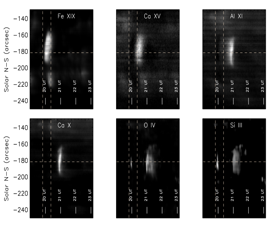
Figure 1: Time-intensity plot of selected ions observed by SUMER. The X-axis is time, the Y-axis is the position along the slit in heliocentric coordinates. The two vertical lines in each panel represent the beginning and the end of the GOES flare. The horizontal line indicates the pixel of the SUMER slit chosen for the analysis. The Si iii 1113.23 Å and O iv 554.08 Å lines are displayed here.

Figure 1 illustrates the behavior of the plasma. Each panel is built in two steps. First, the intensity of a line is measured at all pixels along the slit for each of the 162.5 s-long exposures. Then, these 1-D intensity profiles are placed one next to the other to create a 2-D image, where the X-axis represents time, and the Y-axis represents the coordinate along the slit. GOES start and end times of the flare are added to each panel of Figure 1 as vertical dashed lines. Figure 1 captures the three main features of the flare:

1. The impulsive phase shows a sudden, very localized enhancement of Si iii and O iv line emission, followed after a few minutes by a large and long-lasting brightening of Fe xix line emission;

2. The decay phase lasts far longer than observed by GOES, indicating that X-ray instruments only allow to observe a limited portion of the decay phase of the flare;

3. The final phase of the flare can be observed simultaneously with O iv and Si iii (as well as Ne vi and Ca vii, not shown in the figure).

The presence of two distinct loop sources as responsible of different phases of a solar flare was remarked by Reale et al. (2004), who modeled a flare in Proxima Centauri observed with XMM with two different populations of loops. In a similar way, the initial Si iii and O iv pulses observed by SUMER in the 26 Septemper 2000 flare may be due to a different kind of loops than the rest of the decay phase observed with all the other ions, and thus can not be modeled together with the latter in a single-loop framework.

Feldman et al. (2003) found that the plasma emitting during the decay phase of the flare between 20 UT and 21 UT was close to isothermal, and its temperature decreased exponentially with time from 7.9 MK to 2.5 MK. Then, they reported the simultaneous emission of several ions whose temperature of formation under ionization equilibrium spanned more than one order of magnitude. The light curves of these cooler ions suggest that they are emitted by the cooling post-flare plasma. In fact, Figure 1 shows that the intensity enhancements of Ca x, O iv and Si iii all overlap, and they prolong in time those of Fe xix, Ca xv and Al xi studied by Feldman et al. (2003). To provide quantitative measurements of the relationship among the light curves of all these ions we chose to concentrate on a single pixel along the SUMER slit, shown in Figure 1 by the horizontal dashed line. This pixel corresponds to “position 38” in Feldman et al. (2003). We measured the intensities of all lines in this position as a function of time, and displayed their normalized values in Figure 2. The impulsive phase of the flare is visible by a sudden brightening in Si iii and O iv right before 20 UT, and then the long decay phase studied by Feldman et al. (2003) is apparent from the peak of the Fe xix line emission to that of Al xi.

The surprising feature of Figure 2 is the sudden appearance (at around 21 UT) and co-existence of the emission from Ca x (formed in equilibrium at $\log T=5.7-6.3$), Ca vii ($\log T=5.4-5.9$), Ne vi ($\log T=5.4-5.8$), O iv ($\log T=4.9-5.5$) and Si iii ($\log T=4.3-5.0$). These ions are emitted by a previously cooling, near-isothermal plasma undergoing a series of equilibrium states, and yet cannot be emitted simultaneously by an isothermal plasma in ionization equilibrium as their temperature ranges of formation do not overlap. The most likely explanation to the presence of the emission from these ions is that the cooling post-flare plasma undergoes a thermal instability as it reaches $\approx 2$ MK.

The modeling effort of the present work is aimed at reproducing the light curves of the thermal instability after 21 UT. We are particularly interested at studying the succession of rise and fall of the emission in the colder ions.

2.3 Plasma diagnostics

The plasma temperature was estimated by Feldman et al. (2003) assuming that the plasma evolved through quasi-equilibrium states from right after the impulsive phase (around 20:05 UT, approximately 15 minutes after the GOES beginning of the flare) down to 20:45 UT, so that the shape of the Fe xix and Ca xv light curves could be fitted using the contribution functions of the two lines. The $\log T$ of the plasma was found to evolve linearly with time from an initial $\log T=6.9$ at 20:05 UT to $\log T=6.40$ at 20:45 UT. The free-free emission was observed until 21:05 UT and it allowed to determine that the plasma composition was similar to the standard composition of the solar corona; this means that the plasma in the decay phase of the flare had a local, coronal origin rather than being evaporated from the chromosphere.

The plasma density was determined by Feldman et al. (2003) by using the value of the total emission measure they derived from the free-free radiation and an assumed value of the total length of the flaring plasma along the line of sight. However, there are two ions in the 1097-1119 Å range that emit more than one line: Si iii and O iv. The former provides a ratio which is density sensitive in the $\log N_{e}=10-12$ range ($N_{e}$ in cm^-3), so that we can attempt a crude estimate using the emissivities from the CHIANTI database (Dere et al. 1995, 2009). Si iii emission is observed at the very beginning of the flare, during the impulsive phase, and late in the decay phase. At the beginning of the event the intensity ratio is 0.60$\pm$0.06, corresponding to $\log N_{e}>11.8$ while at the end of the decay phase the ratio is $0.43\pm 0.03$, with little temporal evolution, indicating a density of $\log N_{e}=10.5\pm 0.3$. The density estimate made by Feldman et al. (2003) during the impulsive phase is consistent with the value obtained with the line intensity ratio only if we assume that the actual volume filled by the plasma is very small, indicating a filling factor smaller than unity. During the decay phase, on the contrary, the two estimates agree with each other if we assume a unity filling factor and a length of the line of sight $H$ in the 1″-10″ range. On Sept. 26, 2000 1″ at SOHO’s distance corresponded to $\approx$720 km at the Sun, so that $7.2\times 10^{7}\leq H\leq 7.2\times 10^{8}$ cm.

3 Hydrodynamic modeling and numerical setup

We aim at explaining the evolution of the observed emission through the hydrodynamic modeling of a flare-heated plasma confined in a coronal magnetic flux tube as in Reale & Orlando (2008). We consider semicircular loops with half-length in the range $1.5\times 10^{9}<L<5\times 10^{9}$ cm, typical of active region loops, and constant cross-section area all along the loops. The loops lie on a plane vertical to the solar surface. It is assumed that the loop plasma moves and transports energy only along the magnetic field lines. The plasma evolution can then be described by one-dimensional (1-D) hydrodynamics (e.g., Peres et al. 1982):

$$\frac{\partial\rho}{\partial t}+\frac{\partial\rho u}{\partial s}=0$$ (1)

$$\frac{\partial\rho u}{\partial t}+\frac{\partial(P+\rho u^{2})}{\partial s}=\rho g$$ (2)

$$\frac{\partial\rho E}{\partial t}+\frac{\partial(\rho E+P)u}{\partial s}=\rho ug-\frac{\partial q}{\partial s}+Q(s,t)-n_{e}n_{H}\Lambda(T)$$ (3)

$$\mbox{where \hskip 14.22636pt}E=\epsilon+\frac{1}{2}u^{2}$$

is the total gas energy (internal energy, $\epsilon$, and kinetic energy), $t$ the time, $s$ the coordinate along the loop, $\rho=\mu m_{H}n_{\rm H}$ the mass density, $\mu=1.26$ the mean atomic mass (assuming solar abundances), $m_{H}$ the mass of the hydrogen atom, $n_{\rm H}$ the hydrogen number density, $n_{\rm e}$ the electron number density, $u$ the plasma flow velocity, $P$ the pressure, $g$ the component of gravity parallel to the field lines, $T$ the temperature, $q$ the conductive flux, $Q(s,t)$ a function describing the transient input heating, $\Lambda(T)$ the radiative losses per unit emission measure (Rosner et al. 1978). The radiative losses are assumed from plasma in ionization equilibrium and are set to zero for $T<20000$ K, to ensure the detailed energy balance in the chromosphere. Tests have shown that the simulation results do not change considerably because of local and temporary changes of the radiative losses function, as those due by transient deviations from equilibrium of ionization (Reale & Orlando 2008). We use the ideal gas law, $P=(\gamma-1)\rho\epsilon$, where $\gamma=5/3$ is the ratio of specific heats.

The flare evolution may be faster than ionization and recombination timescales, so that the ionization fraction of the emitting ions may not have enough time to adjust to the rapidly changing plasma temperature (e.g. Golub et al. 1989, Orlando et al. 1999). This effect may be important even in the late phases of the flare. Therefore in our modeling we also compute the ionization fractions of the most important elements (namely He, C, N, O, Ne, Mg, Si, S, Ar, Ca, Fe, Ni), by solving synchronously but independently the continuity equations for each ion species:

$$\frac{\partial n_{i}^{Z}}{\partial t}+\nabla\cdot n_{i}^{Z}\mbox{\bf v}=R_{i}^{Z}~{}~{}~{}~{}~{}~{}~{}~{}\begin{array}[]{l}(Z=1,...,N_{elem})\\ \\ (i=1,...,N_{ion}^{Z})\end{array}$$ (4)

$$\mbox{where}~{}~{}~{}R_{i}^{Z}=n_{e}[n_{i+1}^{Z}\alpha_{i+1}^{Z}+n_{i-1}^{Z}S_{i-1}^{Z}-n_{i}^{Z}(\alpha_{i}^{Z}+S_{i}^{Z})]~{},$$

$n_{i}^{Z}$ is the number density of the $i$-th ion of the element $Z$, $N_{elem}$ the number of elements, $N_{ion}^{Z}$ the number of ionization states of element $Z$, $\alpha_{i}^{Z}$ the collisional and dielectronic recombination coefficients, and $S_{i}^{Z}$ the collisional ionization coefficients (Summers 1974).

As discussed in Reale & Orlando (2008), the heat conduction may become “flux limited” during flares (e.g. Brown et al. 1979), and our model allows for a smooth transition between the classical and saturated conduction fluxes (Dalton & Balbus 1993):

$$q=\left(\frac{1}{q_{\rm spi}}+\frac{1}{q_{\rm sat}}\right)^{-1}~{},$$ (5)

where $q_{\rm spi}=-\kappa(T)\nabla T$ is the classical conductive flux (Spitzer 1962), $\kappa(T)=9.2\times 10^{-7}T^{5/2}$ erg s^-1 K^-1 cm^-1 the thermal conductivity, $q_{\rm sat}=-\mbox{sign}\left(\nabla T\right)~{}5\phi\rho c_{\rm s}^{3}$ the saturated flux, $c_{\rm s}$ the isothermal sound speed. The correction factor $\phi=1$ is set according to the values suggested for the coronal plasma (Giuliani 1984, Borkowski et al. 1989, Fadeyev et al. 2002, and references therein).

The flare is triggered by a heat pulse defined by the function $Q(s,t)=H_{0}\times g(s)\times f(t)$, where $g(s)$ is a Gaussian function:

$$g(s)=\exp[-(s-s_{H})^{2}/(2\sigma_{H}^{2})]$$

and $f(t)$ is a pulse function (see Reale & Orlando 2008 for details). In all our simulations, the heat pulse starts at time $t=0$ and it is switched off after 180 s. We do not change this duration, since the late evolution of the flare is governed mostly by the total energy input, which we tune by changing $H_{0}$.

The model is implemented and solved numerically using the flash code (Fryxell et al. 2000), an adaptive mesh refinement multiphysics code, extended by additional computational modules to handle the plasma thermal conduction (see Orlando et al. 2005 for details of the implementation), the non-equilibrium ionization (NEI) effects (see Reale & Orlando 2008 for the details), the radiative losses, and the heating function.

As for the initial conditions, before the flare the loop plasma is assumed to be in pressure and energy equilibrium according to Serio et al. (1981) and to Orlando et al. (1995). The plasma is very cool and tenuous: the pressure at the base of the corona is $p_{0}=0.055$ dyn cm^-2, which corresponds to a maximum temperature $T_{0}\approx 0.8$ MK at the loop apex, according to the loop scaling laws (Rosner et al. 1978). Since the pressure increases enormously during the flare, the flare evolution is largely independent of these initial conditions. The coronal part of the loop is linked to an isothermal chromosphere at $T_{\rm c}=20000$ K and $0.5\times 10^{9}$cm thick, which acts only as a mass reservoir. All the ion species are assumed to be initially in ionization equilibrium everywhere in the loop.

Since we assume that the loop is symmetric with respect to the vertical axis across the apex, we simulate only half of the loop. For the case $L=3\times 10^{9}$ cm, the computational domain spans a total extension of $3.5\times 10^{9}$ cm, including the chromosphere which has a thickness of $5\times 10^{8}$ cm. At the coarsest resolution, the adaptive mesh algorithm used in the flash code (paramesh; MacNeice et al. 2000) uniformly covers the computational domain with a mesh of $16$ blocks, each with $8$ cells. We allow for 3 levels of refinement, with resolution increasing twice at each refinement level. The refinement criterion adopted (Löhner 1987) follows the changes in density and temperature. With this grid configuration the effective resolution is $\approx 3.4\times 10^{6}$ cm at the finest level, corresponding to an equivalent uniform mesh of $1024$ grid points. We use fixed boundary conditions at $s=0$ and reflecting boundary conditions at $s=s_{\rm max}$ (consistent with the adopted symmetry).

4 Model results and comparison with observations

After some exploration of the parameter space, results that provide a good match to observations are obtained with a loop of half length $L=3\times 10^{9}$ cm, and with a heat pulse of intensity $H_{0}=8$ erg cm^-3 s^-1, Gaussian width and center $\sigma_{H}=10^{8}$ cm and $s_{H}=8\times 10^{8}$ cm, respectively. The heat pulse is therefore located close the loop footpoint i.e. $\approx 3\times 10^{8}$ cm above the transition region. We now discuss this simulation in some detail.

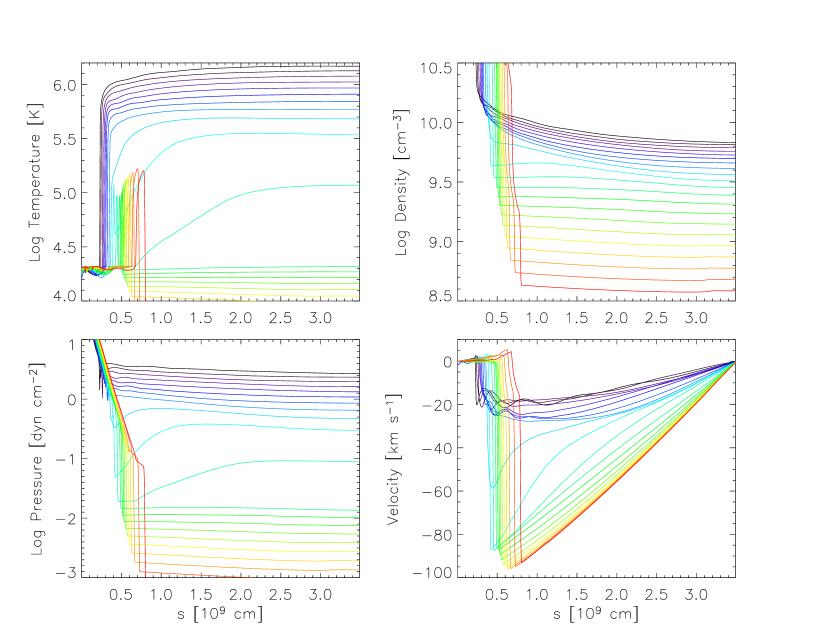
Figure 3: Evolution of temperature, density, pressure and velocity along half of the model loop in the late phases of the flare, when the plasma becomes thermally unstable. The curves are sampled at time intervals of 1 minute between 30 (black line) and 50 (red line) minutes since the heat pulse has been triggered.

The evolution of the flare-heated plasma confined in a coronal loop is well known from previous work (e.g. Nagai 1980, Peres et al. 1982, Cheng et al. 1983, Nagai & Emslie 1984, Fisher et al. 1985, MacNeice 1986, Betta et al. 2001). In particular, the choice of the parameters and the specific model make our results very similar to those described in Reale & Orlando (2008) for the case of heat pulse deposited at the loop footpoints and lasting 180 s. The only difference is that the heating rate is about 5 times larger, leading to a maximum temperature twice as high, i.e. about 20 MK. Since here we focus on the late phases of the flare, we do not enter the details of the initial phases which are similar to those described by Reale & Orlando (2008). We only mention that the loop is rapidly filled by hot plasma and that the plasma begins to cool down by conduction and radiation as soon as the heat pulse stops, but the density still grows for a few minutes. The plasma then drains and cools altogether. Fig. 3 illustrates the evolution of the plasma along half of the model loop from 30 to 50 minutes after the start of the heat pulse. During this phase, the plasma density at the formation temperature of the Si iii lines is in the range $10<\log N_{\rm e}<11$, in agreement with the values inferred from spectroscopic analysis of the data (see Sect. 2.3). The plasma cools down gradually and uniformly along the loop for about 10 minutes but then it suddenly gets thermally unstable and the temperature drops in about 2 minutes by a factor 10, from $\log T\approx 5.5$ to $\log T\approx 4.5$, in the coronal part of the loop. The density decreases more gradually and at a constant rate, so that at $t\sim 40$ min the plasma is cold but still relatively dense. Since the plasma is dramatically out of the hydrostatic equilibrium, it begins to drain more rapidly and its downward velocity increases from $\sim 20$ km/s to $\sim 100$ km/s. A front of relatively hotter and denser plasma ($\log T\approx 5$) develops at the loop footpoints and slowly propagates along the loop.

The trigger of the thermal instability can be explained in terms of the criterion described by Field (1965): below 1 MK the radiative losses begin to increase for decreasing temperature (negative slope) and the density is sufficiently high that the cooling becomes catastrophic.

The presence of the instability is even more clear in the evolution of the loop top temperature. The temperature at the top of the loop is a good proxy of the loop maximum temperature for most of the time (Fig. 3). Fig. 4 shows the loop top temperature and density during the entire duration of the flare. The heat capacity of the loop is initially very small and the temperature increases very rapidly, but it also saturates as well because of the increased losses due to the highly efficient thermal conduction. After the end of the heat pulse, the temperature decreases regularly (exponentially) during most of the first 40 min, and then drops suddenly to $T\sim 20000$ K. Below this temperature, the plasma is assumed to radiate no more, so the thermal evolution for $t>41$ min is outside the scope of the modeling. After the temperature drops, the plasma begins to drain more rapidly and the density also decreases more rapidly (lower panel).

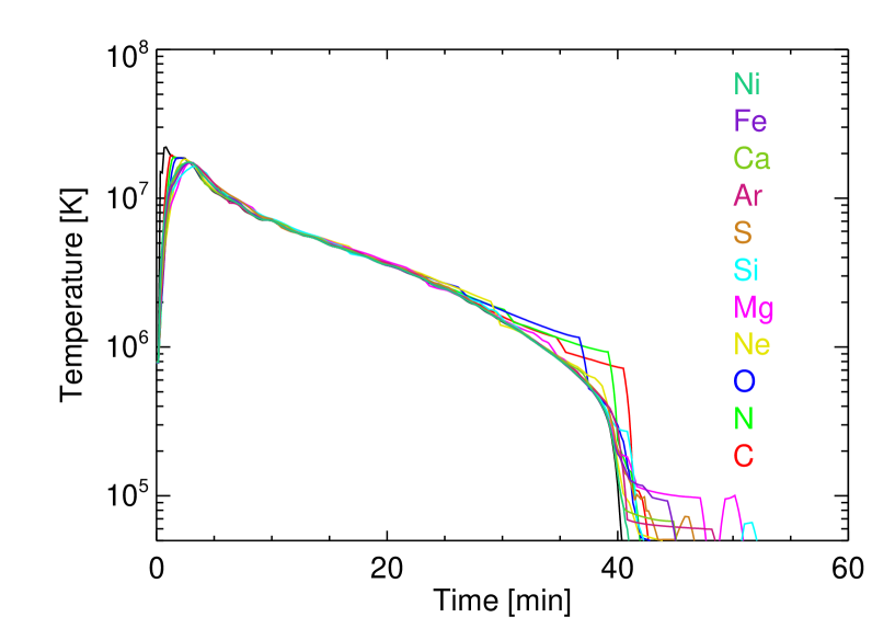
Figure 5: Evolution of element effective temperature T_eff at the loop top during the entire flare evolution. Each color line marks the temperature related to a different element as derived in Reale & Orlando (2008) (see text for details). The black line indicates the electron temperature.

To study the degree of departure from equilibrium in a plasma, Reale & Orlando (2008) introduced for each element an ”effective temperature” (T_eff), as the temperature for which the equilibrium ion abundances of the element best approximates the actual values in the plasma. In case of equilibrium, all elements have the same T_eff and this should equal the electron temperature. Fig. 5 shows the evolution of T_eff at the loop top for the most important ion species: the ion temperatures substantially differ from $T_{\rm e}$ only during the earliest phase of the flare ($t<5$ min) and do not evolve very differently from $T_{\rm e}$ in later phases. We find again some deviations from the ionization equilibrium around the thermal instability ($30<t<40$ min), because the temperature drops abruptly. The instability starts from a hotter status ($\sim 1$ MK) for the light elements C, N, and O ions (when the electron temperature is $\approx 5\times 10^{5}$ K). This temperature drop is mainly due to the fact that the thermal instability occurs in a range of temperature in which the He-like ionization state of these light elements is the most populated. Since the temperature $T_{eff}$ is found as the temperature at which the two most populated ionization states fit those assuming equilibrium of ionization, the NEI effects together with the fact that He-like ions are the most abundant in a broad range of temperatures lead to the observed jump of $T_{eff}$. Note also that $T_{eff}$ for O, N, C drop consecutively in time because the corresponding He-like ionization state forms at lower and lower temperatures during the plasma cooling. Although apparently large, the deviations from equilibrium are so concentrated in time that they do not produce strong effect on the visible emission.

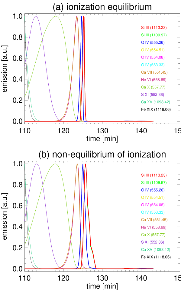
Figure 6: Light curves synthesized in the labelled spectral lines from the flare loop model. The times have been shifted to match the times of the observation. Only the late phases of the flare are shown, the initial time (t = 110 min) corresponds to t=25 min since the start of the heat pulse, and to 20:51 UT in Figure 2. (a) Light curves computed assuming ionization equilibrium. (b) Light curves computed including the effects of non-equilibrium of ionization.

The model allows us to predict the light curves of the observed lines. Fig. 6 shows them during the development of the thermal instability in the late phase of the flare, both assuming and not assuming ionization equilibrium. Time origin and range have been adjusted to allow a direct comparison with the observed light curves. Fig. 6 confirms that the effects of deviations from ionization equilibrium are not important: only the light curves of the coldest lines (Si iii, O iv) are affected, by being slightly broader, i.e. their decay is slightly slower in the latest phases. Thus, both panels can be compared to observations and they show the same results: first, the time sequence and the relative start time of the light curves of each line are both in very good agreement with observations (within 1-2 min), with the exception of the hottest lines (Ca xv); and second, the observed light curves are considerably broader than the predicted ones, i.e. both the rise and the decay are slower than modelled.

We have found that the timing and line sequence could not be reproduced with the same accuracy with other model parameters, and in particular longer ($5\times 10^{9}$ cm) loops, more (to a maximum temperature of 25 MK) or less (10 MK) intense heating, and also a heat pulse deposited at the loop apex. We define the root mean square time distance of the simulated and observed peak between lines as a goodness-of-fit parameter:

$$\sigma_{t}=\sum_{i}\sqrt{\left(t_{sim}-t_{obs}\right)^{2}_{i}}$$

where $t_{sim}$ and $t_{obs}$ are the times of the peak of the i-th line light curves measured in the simulation and in the observation, respectively. Here we align the times to be the same for the peak of the Si iii line. We measure $\sigma_{t}$ over the coolest lines (from S xi to Si iii).

We have found that the value of the best-fit model is $\sigma_{t}\sim 4$ min, while for all others values between 9 and 50 min. For the best-fit model, each peak of the (cool) model light curves is within 5 min from respective peak of the observed light curves. Indeed, we have found $\sigma_{t}\sim 4$ min also from a simulation with a shorter loop $L=1.5\times 10^{9}$ cm and maximum temperature of 20 MK.

One more constraint from the observation is the absolute intensity of the line emission. To compute the line intensity from the simulation results we need to make an assumption on the path length $H$ along the line of sight. For $L=3\times 10^{9}$ cm, we find that the path length that matches the measured one is between $1$ and $2\times 10^{8}$ cm for the lines marking the thermal instability (from the warm S xi to the cool Si iii). This is in agreement with the estimate of $H$ made in Section 2.3, and it is also compatible with a loop cross-section diameter of the order of 10% of the loop length, as typical of coronal loops. For the shorter loop ($L=1.5\times 10^{9}$ cm) the path length is larger ($1.5-4\times 10^{8}$ cm) but still well within the range of values found in Section 2.3. In this case, the flaring structure would have more the aspect of a flaring loop arcade. Since we have reasons to believe that the flare occurs in a multi-structured loops, both scenarios seem possibile. Morevover, these loop lengths are compatible with the vertical height corresponding to the SUMER slit position above the limb. Overall, we can say that the loop length, and the heat intensity and position are relatively well constrained and provide a reasonably self-consistent scenario.

None of the explored single loop models has been able to reproduce the observed ”broad” light curves, i.e. the observed light curves change more slowly than those obtained from the hydrodynamic simulations.

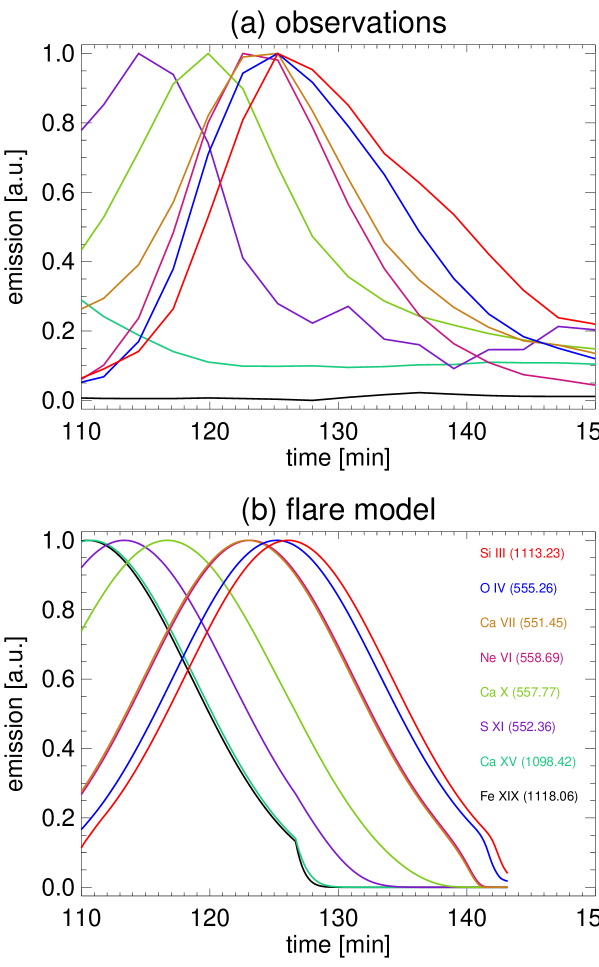
Figure 7: Comparison of (a) observed light curves with (b) best model light curves obtained assuming a distribution of heat pulses in different loop structures. In particular, curves in (b) are obtained convolving those in Fig. 6b with a Gaussian whose width is 8 min. The initial time (t = 110 min) corresponds to t=25 min since the start of the heat pulse, and to 20:51 UT in Figure 2.

The agreement is further improved if we assume that the flaring region is not a single monolithic loop, but it is substructured into a bundle of loops or loop strands, each of the same length as the loop we modeled. Each component is heated at a different time, and the time distribution of the heating pulses is assumed to be Gaussian with $\sigma=8$ minute width. We derive the related line light curves simply as the convolution of the single loop light curves with the (same) Gaussian. The results are shown in Fig. 7 and compared to observations. The predicted light curves are now in closer agreement as far as time sequence, time evolution and time scale are concerned.

We are unable to, and do not pretend to, constrain the number of loops or strands. The convolution with the Gaussian means that at any time the line intensities are the same relative to the others (i.e. the ratio is unchanged). So there is only a scale factor that changes in time, which is a volume factor. This implies that all loops/strands are heated in the same way, and only the number of heated loops/strands first progressively increases and then progressively decreases. We cannot claim that this is the only way to produce this effect, but we can certainly say that this is a very simple way to do that, with very few free parameters (only the rate of involved strands).

Although fine details such as the asymmetry between rise and decay of the light curves can still be improved, overall we can conclude that this agreement is evidence of a thermally unstable plasma confined in a substructured loop system undergoing cooling after a flare.

It is worth noting that the thermal instability occurs at $t\sim 40$ min after the heat pulse, while the observation indicates that it should occur $\sim 60$ min after the start of the flare (see Fig.2). The discrepancy between the flare start time and the start of the heat pulse, as well as the disagreement in the time profile of hot lines, may be better resolved if the model can produce a temperature time profile that at first decreases from 20 MK more rapidly but stays longer (by $\simeq$20 min) above $\simeq$1 MK before going into thermal instability. This appears to be limited by the current setting of the model for the energy balance.

5 Discussion and Conclusions

This work aims at explaining the peculiar light curves of several UV lines in the late phases of a flare observed with SOHO/SUMER. In particular, our target is the appearance of several spectral lines emitted by plasma in a wide range of temperature in a relatively short time. The scope of this work is modeling the post-flare phase and therefore we do not attempt at reproducing the initial phases of the flare.

We show that light curves are well reproduced by the hydrodynamic evolution of flaring plasma confined in a closed loop system triggered by a strong heat pulse. In particular, the sudden, almost simultaneous appearance of the emission of chromospheric and transition region ions formed more than one order of magnitude apart in temperature is due to the fact that late in the cooling phase the plasma becomes thermally unstable, because the radiative losses increase rapidly below 1 MK, and its temperature drops rapidly by one order of magnitude in a couple of minutes along most of the loop. A good relative timing and order of appearance of the light curves of each line is obtained with a standard flare loop model considering a loop half-length of $\leq 3\times 10^{9}$ cm, and a heat pulse lasting 3 min and deposited in the corona, close to the loop footpoints. The heating rate is such as to have a flare maximum temperature of about 20 MK.

Better agreement of the duration of the light curve of each line is obtained if we assume that the flare occurs in a bundle of subloops of equal length (a stranded loop or a loop arcade). If each substructure is assumed to be heated at a different time, the predicted light curves can be lengthened to match the observed ones. This is consistent with the slit intercepting several concentric arches that undergo independently the same evolution, so that we see the envelope of this close sequence of events. The time scale of the distribution of the events is about 8 min, that indicates a propagation speed of the trigger signal of $\sim 10$ km/s over a length scale of $\sim 10^{9}$ cm. This result might be consistent with the presence of fine heat substructuring during flares (e.g. Antiochos & Krall 1979, Reeves & Warren 2002, Warren 2006).

The occurrence of the thermal instability is a necessary ingredient to explain the observations. However, the effects of such instability on the ion fractions of the major elements are rather limited, contrarily to our initial expectations. The reason of such limited departures is the relatively large density of the cooling plasma, which shortens the ionization and recombination times scales enough to allow the plasma to efficiently adjust its ionization status to the rapidly decreasing electron temperature (e.g. Golub et al. 1989).

We do not reproduce all the details of the observations. In particular, the light curves of the hot lines are not well reproduced, and probably would need a more complete analysis of the entire flare event, which is not the target of this study.

The main limitation of the present work is the lack of spatial information on the flaring region, and better constraints on the heating location and timing, and on the properties of the flaring loops systems, can be obtained by combining the present modeling with flares observed with the EVE spectrometer and the AIA imaging system on the SDO.

Ion	Wavelength (Å)	$\log T_{max}$	Transition
Si iii	1109.97	4.7	$3s3p$ 3P1 - $3s3d$ 3D1,2
Si iii	1113.23	4.7	$3s3p$ 3P2 - $3s3d$ 3D1,2,3
O iv	553.33	5.2	$2s^{2}$$2p$ 2P1/2 - $2s2p^{2}$ 2P3/2
O iv	554.08	5.2	$2s^{2}$$2p$ 2P1/2 - $2s2p^{2}$ 2P1/2
O iv	554.51	5.2	$2s^{2}$$2p$ 2P3/2 - $2s2p^{2}$ 2P3/2
O iv	555.26	5.2	$2s^{2}$$2p$ 2P3/2 - $2s2p^{2}$ 2P1/2
Ne vi	558.69	5.6	$2s^{2}$$2p$ 2P1/2 - $2s2p^{2}$ 2D3/2
Ca vii	551.45	5.7	$3s^{2}$$3p^{2}$ 3P2 - $3s3p^{3}$ 3P1,2
Ca x	557.77	5.9	$3s$ 2S1/2 - $3p$ 2P3/2
Al xi	550.03	6.1	$2s$ 2S1/2 - $2p$ 2P3/2
S xi	552.36	6.3	$2s^{2}$$2p^{2}$ 3P1 - $2s2p^{3}$ 5S2
Na x	1111.77	6.3	$1s2s$ 3S1 - $1s2p$ 3P2
Ca xv	1098.42	6.6	$2s^{2}$$2p^{2}$ 3P1 - $2s^{2}$$2p^{2}$ 1D2
Fe xix	1118.06	7.0	$2s^{2}$$2p^{4}$ 3P2 - $2s^{2}$$2p^{4}$ 3P1

Table 1: Lines included in the SUMER spectra. $T_{max}$ is the temperature of maximum abundance of the ion, from Bryans et al. (2009). Lines with wavelengths smaller than 1000 Å were observed in second order.

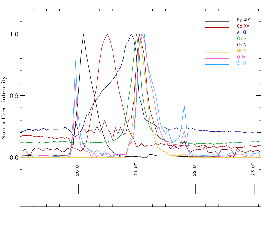
Figure 2: Normalized intensities of several lines measured as a function of time from the selected pixel along the SUMER slit. The Si iii 1113.23 Å and O iv 554.08 Å lines are displayed here.

Figure 4: Evolution of the temperature (top panel) and density (lower panel) at the top of the loop throughout the modelled flare duration.

References

- (1) Antiochos, S. K., & Krall, K. R. 1979, ApJ, 229, 788
- (2) Antiochos, S. K. 1980, ApJ, 236, 270
- (3) Betta, R. M., Peres, G., Reale, F., & Serio, S. 2001, A&A, 380, 341
- (4) Borkowski, K. J., Shull, J. M., & McKee, C. F. 1989, ApJ, 336, 979
- (5) Brown, J. C., Spicer, D. S., & Melrose, D. B. 1979, ApJ, 228, 592
- (6) Bryans, P., Landi, E., & Savin, D.W. 2009, ApJ, 691, 1540
- (7) Cheng, C.-C., Oran, E. S., Doschek, G. A., Boris, J. P., & Mariska, J. T. 1983, ApJ, 265, 1090
- (8) Dalton, W. W., & Balbus, S. A. 1993, ApJ, 404, 625
- (9) De Groof, A., Berghmans, D., van Driel-Gesztelyi, L., & Poedts, S. 2004, A&A, 415, 1141
- (10) Dere, K.P., Landi, E., Mason, H.E., Monsignori Fossi, B.C., & Young, P.R. 1997, A&ASS, 125, 149
- (11) Dere, K.P., Landi, E., Young, P.R., Del Zanna, G., Landini, M., & Mason, H.E. 2009, A&A, 498, 915
- (12) Fadeyev, Y. A., Le Coroller, H., & Gillet, D. 2002, A&A, 392, 735
- (13) Feldman, U., Landi, E., Doschek, G.A., Dammasch, I., & Curdt, W. 2003, ApJ, 593, 1226
- (14) Field, G.B. 1965, ApJ, 142, 531
- (15) Fisher, G. H., Canfield, R. C., & McClymont, A. N. 1985, ApJ, 289, 414
- (16) Fryxell, B. et al. 2000, ApJS, 131, 273
- (17) Giuliani, J. L. 1984, ApJ, 277, 605
- (18) Golub, L., Hartquist, T. W., & Quillen, A. C. 1989, Sol. Phys., 122, 245
- (19) Kaastra, J. S., & Mewe, R. 2000, in Atomic Data Needs for X-ray Astronomy, p. 161
- (20) Karpen, J.T., Antiochos, S.K., & Klimchuk, J.A. 2006, ApJ, 637, 531
- (21) Klimchuk, J.A., Karpen, J.T., & Antiochos, S.K. 2010, ApJ, 714, 1239
- (22) Löhner, R. 1987, Comp. Meth. Appl. Mech. Eng., 61, 323
- (23) MacNeice, P. 1986, Sol. Phys., 103, 47
- (24) MacNeice, P., Olson, K. M., Mobarry, C., de Fainchtein, R., & Packer, C. 2000, Comp. Phys. Comm., 126, 330
- (25) Mewe, R., Gronenschild, E. H. B. M., & van den Oord, G. H. J. 1985, A&AS, 62, 197
- (26) Müller, D.A.N., De Groof, A., Hansteen, V.H., & Peter, H. 2005, A&A, 436, 1067
- (27) Nagai, F. 1980, Sol. Phys., 68,351
- (28) Nagai, F., & Emslie, A. G. 1984, ApJ, 279, 896
- (29) Orlando, S., Peres, G., & Serio, S. 1995, A&A, 294, 861
- (30) Orlando, S., Bocchino, F., & Peres, G. 1999, A&A, 346, 1003
- (31) Orlando, S., Peres, G., Reale, F., Bocchino, F., Rosner, R., Plewa, T., & Siegel, A. 2005, A&A, 444, 505
- (32) Peres, G., Serio, S., Vaiana, G. S., & Rosner, R. 1982, ApJ, 252, 791
- (33) Raymond, J. C., & Smith, B. W. 1977, ApJS, 35, 419
- (34) Reale, F., & Orlando, S. 2008, ApJ, 684, 715
- (35) Reale, F., Güdel, Peres, G., & Audard, M. 2004, A&A, 416, 733
- (36) Reeves, K. K., & Warren, H. P. 2002, ApJ, 578, 590
- (37) Rosner, R., Tucker, W. H., & Vaiana, G. S. 1978, ApJ, 220, 643
- (38) Serio, S., Peres, G., Vaiana, G. S., Golub, L., & Rosner, R. 1981, ApJ, 243, 288
- (39) Spitzer, L. 1962, Physics of Fully Ionized Gases (New York: Interscience, 1962)
- (40) Summers, H. P. 1974, Internal Mem., Vol. 367 (Astrophysics Research Div., Appleton Lab., Abingdon, Oxon)
- (41) Warren, H. P. 2006, ApJ, 637, 522
- (42) Wilhelm, K. et al. 1995, Sol. Phys., 162, 189
- (43) Woods, T.N., Champerlin, P., Eparvier, F.G., et al. 2010, Sol. Phys., in press