Numerical study of higher order analogues of the Tracy–Widom distribution

Abstract

We study a family of distributions that arise in critical unitary random matrix ensembles. They are expressed as Fredholm determinants and describe the limiting distribution of the largest eigenvalue when the dimension of the random matrices tends to infinity. The family contains the Tracy–Widom distribution and higher order analogues of it. We compute the distributions numerically by solving a Riemann–Hilbert problem numerically, plot the distributions, and discuss several properties that they appear to exhibit.

1 Introduction

Consider the space of Hermitian $n\times n$ matrices with a probability measure of the form

$$\frac{1}{Z_{n}}e^{-n\,{\rm tr\,}V(M)}dM,$$ (1.1)

where $dM$ is the Lebesgue measure defined by

$$dM=\prod_{j=1}^{n}M_{jj}\prod_{i<j}d{\rm Re\,}M_{ij}d{\rm Im\,}M_{ij},$$

and where the external field $V$ is a real analytic function with sufficient growth at $\pm\infty$. The quadratic case $V(M)=\frac{1}{2}M^{2}$ corresponds to the Gaussian Unitary Ensemble (GUE) and consists of matrices with independent Gaussian entries. The probability measure (1.1) is invariant under conjugation with a unitary matrix and induces a probability measure on the matrix eigenvalues given by

$$\frac{1}{\tilde{Z}_{n}}\prod_{i<j}(\lambda_{i}-\lambda_{j})^{2}\prod_{j=1}^{n}e^{-nV(\lambda_{j})}d\lambda_{j}.$$ (1.2)

The large $n$ limit of the average counting measure of the eigenvalues of a random matrix (hereafter referred to as the limiting mean eigenvalue distribution) exists and is characterized as the unique measure $\mu_{V}$ which minimizes the logarithmic energy [7]

$$I_{V}(\mu)=\iint\log\frac{1}{|x-y|}d\mu(x)d\mu(y)+\int V(x)d\mu(x),$$ (1.3)

among all probability measures $\mu$ on $\mathbb{R}$. The equilibrium measure $\mu_{V}$ depends on the external field $V$ and is supported on a finite union of intervals $\cup_{j=1}^{\ell}[a_{j},b_{j}]$, with $\ell,a_{j},b_{j}$ depending on $V$. It is absolutely continuous with a density $\psi_{V}$ of the form [10]

$$\psi_{V}(x)=\prod_{j=1}^{\ell}\sqrt{(b_{j}-x)(x-a_{j})}\ h(x),\qquad x\in\cup_{j=1}^{\ell}[a_{j},b_{j}],$$ (1.4)

where $h(x)$ is a real analytic function on $\mathbb{R}$. Generically [14], $h$ has no zeros on the support and in particular at the endpoints $a_{j},b_{j}$, so that the equilibrium density has square root vanishing at the endpoints. However, there exist singular external fields $V$ which are such that $h(b_{j})=0$ (or $h(a_{j})=0$). If $h(b_{j})=0$, then necessarily an odd number of derivatives vanish: we have

$$h^{\prime}(b_{j})=\cdots=h^{(2k-1)}(b_{j})=0,\qquad h^{(2k)}(b_{j})\neq 0,$$ (1.5)

for $k\in\mathbb{N}$. The value $k=0$ corresponds to the generic square-root behavior and $k=1$ to the first type of critical behavior where $\psi_{V}(x)\sim c(b_{j}-x)^{5/2}$ as $x\nearrow b_{j}$.

Example 1.1

The simplest critical case $k=1$ occurs, e.g., for the critical quartic potential

$$V(x)=\frac{1}{20}x^{4}-\frac{4}{15}x^{3}+\frac{1}{5}x^{2}+\frac{8}{5}x.$$ (1.6)

The limiting mean eigenvalue density is then supported on $[-2,2]$ and given by [5]

$$\psi_{V}(x)=\frac{1}{10\pi}(x+2)^{1/2}(2-x)^{5/2},\qquad\mbox{$x\in[-2,2]$}.$$ (1.7)

Example 1.2

The general situation $k\in\mathbb{N}$ can be realized for instance with the following family of polynomials,

$$V_{k}(x)=2\cdot\frac{(2k+2)!}{\left(-\frac{1}{2}\right)_{2k+2}}\sum_{\ell=0}^{2k+1}\frac{(-1)^{\ell}(\ell+\frac{1}{2})_{2k+1-\ell}}{(2k+1-\ell)!(\ell+1)}x^{\ell+1},$$ (1.8)

where $(a)_{m}=a\cdot(a+1)\cdots(a+m-1)$ is the Pochhammer symbol. The corresponding limiting mean eigenvalue densities are given by

$$\psi_{k}(x)=-\frac{(2k+2)!}{\pi\left(-\frac{1}{2}\right)_{2k+2}}x^{1/2}(1-x)^{2k+1/2},\qquad\mbox{$x\in[0,1]$}.$$ (1.9)

This can be verified by substituting (1.9) into the variational conditions that characterize the equilibrium measures in external field $V_{k}$. These conditions reduce to the equation

$$2\mathop{\hskip 1.16664pt\vbox{\hrule width=3.50002pt,height=0.5pt,depth=0.5pt}\hskip-4.66666pt}\mskip-3.0mu\intop\nolimits_{0}^{1}\frac{\psi_{k}(s)}{x-s}ds=V_{k}^{\prime}(x),\qquad\mbox{ for $x\in(0,1)$},$$

which is readily verified.

The random matrix ensembles under consideration are known to have eigenvalues following a determinantal point process with a kernel of the form [7]

$$K_{n}(x,y)=\frac{e^{-\frac{n}{2}V(x)}e^{-\frac{n}{2}V(y)}}{x-y}\frac{\kappa_{n-1}}{\kappa_{n}}(p_{n}(x)p_{n-1}(y)-p_{n}(y)p_{n-1}(x)),$$ (1.10)

where $p_{j}$ is the degree $j$ orthonormal polynomial with respect to the weight $e^{-nV(x)}$ on $\mathbb{R}$; $\kappa_{j}$ is its leading coefficient. Near a right endpoint $b$ of the support for which $k=0$, it was proved [11, 8] that the large $n$ limit of the re-scaled kernel is the Airy kernel:

$$\lim_{n\to\infty}\frac{1}{cn^{2/3}}K_{n}\left(b+\frac{u}{cn^{2/3}},b+\frac{v}{cn^{2/3}}\right)=K^{(0)}(u,v),$$ (1.11)

uniformly for $u,v\geq-L$, $L>0$, where $c=c_{V}$ and $K^{(0)}$ is the Airy kernel

$$K^{(0)}(u,v)=\frac{{\rm Ai\,}(u){\rm Ai\,}^{\prime}(v)-{\rm Ai\,}(v){\rm Ai\,}^{\prime}(u)}{u-v}.$$ (1.12)

The limit of the probability that the largest eigenvalue is smaller than $b+\frac{s}{cn^{2/3}}$ is given by a Fredholm determinant:

$$\lim_{n\to\infty}{\rm Prob}\left(cn^{2/3}(\lambda_{n}-b)<s\right)=\det(I-K_{s}^{(0)}),$$ (1.13)

where $K_{s}^{(0)}$ denotes the Airy-kernel trace-class operator acting on $L^{2}(s,+\infty)$. The right hand side of the above equation is the Tracy–Widom distribution [19], which can be written in the form

$$\det(I-K_{s}^{(0)})=\exp\left(-\int_{s}^{+\infty}(y-s)q_{0}^{2}(y)dy\right),$$ (1.14)

where $q_{0}$ is the Hastings–McLeod solution $q_{0}$ of the Painlevé II equation

$$q_{xx}=xq+2q^{3}.$$ (1.15)

This solution [13] is characterized by the asymptotic conditions

$$q_{0}(x)\sim{\rm Ai\,}(x), x\to+\infty$$ as , (1.16)

$$q_{0}(x)=\sqrt{\frac{-x}{2}}\left(1+\frac{1}{8x^{3}}+{\cal O}\left(x^{-6}\right)\right), x\to-\infty$$ as . (1.17)

If $b$ is a right endpoint of the support for which $k=1$, i.e. (1.5) holds with $k=1$ and $b_{j}=b$, the kernel has a different limit. It was showed in [6], see also [3, 4], that there exists a limiting kernel $K^{(1)}$ such that

$$\lim_{n\to\infty}\frac{1}{cn^{2/7}}K_{n}\left(b+\frac{u}{cn^{2/7}},b+\frac{v}{cn^{2/7}}\right)=K^{(1)}(u,v),$$ (1.18)

uniformly for $u,v$ in compact subsets of the real line. Since both sides of this equation tend to $0$ rapidly as $u$ or $v$ tends to $+\infty$, this result can be extended to a uniform statement for $u,v\geq-L$, $L>0$, which implies

$$\lim_{n\to\infty}{\rm Prob}\left(cn^{2/7}(\lambda_{n}-b)<s\right)=\det(I-K_{s}^{(1)}),$$ (1.19)

where $K_{s}^{(1)}$ is the trace class operator with kernel $K^{(1)}$ on $(s,+\infty)$. In more complicated double scaling limits, where $V$ is not fixed but depends on $n$ in a critical way, a limiting kernel $K^{(1)}(u,v;t_{0},t_{1})$ depending on two parameters was obtained. Those double scaling limits can describe phase transitions where the number of intervals in the support of the limiting mean eigenvalue distributions changes. If we consider an external field $V=V_{t}$ depending on a parameter $t$, it can happen that the support consists of two intervals for $t<1$, but of only one interval for $t=1$. This happens for example when two intervals approach each other and simultaneously one of the intervals shrinks in the limit $t\searrow 1$. Such phase transitions are covered by the kernels $K^{(1)}(u,v;t_{0},t_{1})$ with non-zero parameters $t_{0},t_{1}$.

The kernels $K^{(1)}(u,v;t_{0},t_{1})$ are related to the second member of the Painlevé I hierarchy, but are most easily characterized in terms of a Riemann-Hilbert (RH) problem. We will give more details about this in the next section.

Although no proofs have been given for $k>1$, when considering in more detail the results and methods in [6], one expects a result of the form

$$\lim_{n\to\infty}\frac{1}{cn^{2/(4k+3)}}K_{n}\left(b+\frac{u}{cn^{2/(4k+3)}},b+\frac{v}{cn^{2/(4k+3)}}\right)=K^{(k)}(u,v;t_{0},\dots,t_{2k-1}),$$ (1.20)

for general $k>1$, where the kernel now depends on $2k$ parameters, and

$$\lim_{n\to\infty}{\rm Prob}\left(cn^{2/(4k+3)}(\lambda_{n}-b)<s\right)=\det(I-K_{s}^{(k)}(t_{0},\dots,t_{2k-1})).$$ (1.21)

The kernels $K^{(k)}$ are related to the Painlevé I hierarchy and will be characterized in the next section in terms of a RH problem. It was proved in [5] that the Fredholm determinant $\det(I-K_{s}^{(k)}(t_{0},\dots,t_{2k-1}))$ can be expressed explicitly in terms of a distinguished solution to the equation of order $4k+2$ in the second Painlevé hierarchy, and in addition asymptotics for $\det(I-K_{s}^{(k)}(t_{0},\dots,t_{2k-1}))$ as $s\to\pm\infty$ were obtained. The asymptotics at $+\infty$ can be derived relatively easy from asymptotic properties of the kernel $K^{(k)}$ and are given by

$$\log\det(I-K_{s}^{(k)}(t_{0},\dots,t_{2k-1}))={\cal O}(e^{-cs^{\frac{4k+3}{2}}}),\qquad\mbox{ as $s\to+\infty$}.$$ (1.22)

The asymptotics as $x\to-\infty$ are more subtle and require a detailed analysis of the Fredholm determinants. In the simplest case $t_{0}=\cdots=t_{2k-1}=0$, they are given by

$$\log\det(I-K_{s}^{(k)})=-\frac{1}{4(4k+3)}\frac{\Gamma(2k+\frac{3}{2})^{2}}{\Gamma(\frac{3}{2})^{2}\Gamma(2k+2)^{2}}|s|^{4k+3}\\ -\frac{2k+1}{8}\log|s|+\chi^{(k)}+{\cal O}(|s|^{-\frac{4k+3}{2}}),\qquad\mbox{ as $s\to-\infty$,}$$ (1.23)

where $\Gamma(x)$ is Euler’s $\Gamma$-function. The constant $\chi^{(k)}$ has no explicit expression, except for $k=0$, where it was proved in [9, 1] that $\chi^{(0)}=\frac{1}{24}\log 2+\zeta^{\prime}(-1)$, and $\zeta(s)$ is the Riemann zeta function.

The goal of this paper is to set up a numerical scheme for computing the Fredholm determinants $\det(I-K_{s}^{(k)}(t_{0},\dots,t_{2k-1}))$, which will allow us to draw plots of the distributions and their densities, to verify formulas (1.22) and (1.23) numerically, to compute numerical values for the constants $\chi^{(k)}$, and to formulate a number of questions about the analytic properties of the distributions (monotonicity, inflection points), based on a closer inspection of the plots. In the next section, we define the kernels in a precise way using a RH problem. This RH characterization will also be used for the numerical analysis which we explain in more detail in Section 3. In Section 4 finally, we show plots of the distributions $\det(I-K_{s}^{(k)})$ and their densities for several values of $k$ and the parameters $t_{0},\ldots,t_{2k-1}$, and we will formulate a number of open problems.

2 Riemann–Hilbert characterization of the kernels

The kernels $K^{(k)}$ have the form

$$K^{(k)}(u,v;t_{0},\ldots,t_{2k-1})=\frac{\Phi_{1}^{(2k)}(u)\Phi_{2}^{(2k)}(v)-\Phi_{1}^{(2k)}(v)\Phi_{2}^{(2k)}(u)}{-2\pi i(u-v)},$$ (2.1)

where the functions $\Phi_{j}^{(2k)}(w)=\Phi_{j}^{(2k)}(w;t_{0},\ldots,t_{2k-1})$ can be characterized in terms of a RH problem.

RH problem for $\Phi$

Figure 1: The jump contour $\Gamma$ and the jump matrices for $\Phi$.

• $\Phi=\Phi^{(2k)}:\mathbb{C}\setminus\Gamma\to\mathbb{C}^{2\times 2}$ is analytic, with

  $$\Gamma=\cup_{j=1}^{4}\Gamma_{j}\cup\{0\},\qquad\Gamma_{1}=\mathbb{R}^{+},\quad\Gamma_{3}=\mathbb{R}^{-},\quad\Gamma_{2}=e^{\frac{-i\pi}{4k+3}}\mathbb{R}^{-},\quad\Gamma_{4}=e^{\frac{i\pi}{4k+3}}\mathbb{R}^{-},$$

  oriented as in Figure 1.

• $\Phi$ has continuous boundary values $\Phi_{+}$ as $\zeta$ approaches $\Gamma\setminus\{0\}$ from the left, and $\Phi_{-}$, from the right. They are related by the jump conditions

  $$\Phi_{+}(\zeta)=\Phi_{-}(\zeta)S_{j},\qquad\mbox{ for $\zeta\in\Gamma_{j}$,}$$ (2.2)

  where

  $$S_{1}=\begin{pmatrix}1&1\\ 0&1\end{pmatrix},$$ (2.3)

  $$S_{2}=S_{4}=\begin{pmatrix}1&0\\ 1&1\end{pmatrix},$$ (2.4)

  $$S_{3}=\begin{pmatrix}0&1\\ -1&0\end{pmatrix}.$$ (2.5)

• $\Phi$ has the following behavior as $\zeta\to\infty$:

  $$\Phi(\zeta)=\zeta^{-\frac{1}{4}\sigma_{3}}N\left(I+h\sigma_{3}\zeta^{-1/2}+{\cal O}(\zeta^{-1})\right)e^{-\theta(\zeta)\sigma_{3}},$$ (2.6)

  where $h=h(t_{0},\ldots,t_{2k-1})$ is independent of $\zeta$, $\sigma_{3}$ is the Pauli matrix $\begin{pmatrix}1&0\\ 0&-1\end{pmatrix}$, $N$ is given by

  $$N=\frac{1}{\sqrt{2}}\begin{pmatrix}1&1\\ -1&1\end{pmatrix}e^{-\frac{1}{4}\pi i\sigma_{3}},$$ (2.7)

  and

  $$\theta(\zeta;t_{0},\ldots,t_{2k-1})=\frac{2}{4k+3}\zeta^{\frac{4k+3}{2}}-2\sum_{j=0}^{2k-1}\frac{(-1)^{j}t_{j}}{2j+1}\zeta^{\frac{2j+1}{2}},$$ (2.8)

  where the fractional powers are the principal branches analytic for $\zeta\in\mathbb{C}\setminus(-\infty,0]$ and positive for $\zeta>0$.

• $\Phi$ is bounded near $0$.

It was proved in [5] that this RH problem is uniquely solvable for any real values of $t_{0},\ldots,t_{2k-1}$. The functions $\Phi_{1}=\Phi_{1}^{(2k)}$ and $\Phi_{2}=\Phi_{2}^{(2k)}$ appearing in (2.1) are the analytic extensions of the functions $\Phi_{11}$ and $\Phi_{21}$ from the sector in between $\Gamma_{1}$ and $\Gamma_{2}$ to the entire complex plane. Alternatively they can be characterized as fundamental solutions to the Lax pair associated to a special solution to the $2k$-th member of the Painlevé I hierarchy. We will not give details concerning this alternative description, since the RH characterization is more direct and more convenient for our purposes.

Remark 2.1

The description in terms of differential equations in the PI hierarchy presents the possibility of computing these distributions using ODE solvers. However, similar to the Hastings–McLeod solution (see [18]), these solutions are inherently unstable; hence, applying this approach in practice would require the use of high precision arithmetic, which is too computationally expensive to be practical. On the other hand, the representation in terms of a RH problem is numerically stable, and therefore is reliable.

Not only the kernel $K^{(k)}$ can be described in terms of a RH problem, but also the logarithmic derivative of the Fredholm determinant can be expressed in terms of a RH problem, which shows similarities with the above one, but is nevertheless genuinely different. We have a formula of the form

$$\frac{d}{ds}\log\det(I-K_{s}^{(k)}(t_{0},\ldots,t_{2k-1}))=\frac{1}{2\pi i}\left.\left(X_{s}^{-1}(\zeta)X_{s}^{\prime}(\zeta)\right)_{21}\right|_{\zeta\searrow s},$$ (2.9)

where $X_{s}$ is the unique solution to a RH problem, see [5, Section 2].

This representation provides relative accuracy, whereas the representation as a Fredholm determinant only provides absolute accuracy [2]. However, it requires solving a RH problem for each point of evaluation $s$ and numerical indefinite integration to recover the distributions. Therefore, the expression in terms of a Fredholm determinant is more computationally efficient.

3 Numerical study of the distributions

We will compute the higher order Tracy–Widom distributions by calculating $\Phi$ numerically, using the methodology of [16, 15]. Consider the following canonical form for a RH problem:

Canonical form for RH problem for $\Psi$

• $\Psi:\mathbb{C}\setminus\overline{\Gamma}\to\mathbb{C}^{2\times 2}$ is analytic, where $\overline{\Gamma}$ is an oriented contour which is the closure of the set $\Gamma=\Gamma_{1}\cup\cdots\cup\Gamma_{\ell}$ whose connected components can be Möbius-transformed to the unit interval $M_{i}:\Gamma_{i}\rightarrow(-1,1)$, with junction points $\Gamma^{*}=\overline{\Gamma}\setminus\Gamma$.

• $\Psi$ has continuous boundary values $\Psi_{+}$ as $\zeta$ approaches $\Gamma$ from the left, and $\Psi_{-}$, from the right. For a given function $G$, they are related by the jump condition

  $$\Psi_{+}(\zeta)=\Psi_{-}(\zeta)G(\zeta).$$ (3.1)

• As $\zeta\to\infty$, we have $\lim\Psi(\zeta)=I$.

• $\Psi$ is bounded near $\Gamma^{*}$.

Define the Cauchy transform

$${\cal C}_{\Gamma}f(\zeta)={1\over 2\pi i}\int_{\Gamma}{f(t)\over t-\zeta}dt,$$

and denote the limit from the left (right) for $\zeta\in\Gamma$ by ${\cal C}_{\Gamma}^{+}$ (${\cal C}_{\Gamma}^{-}$). We represent $\Psi$ in terms of the Cauchy transform of an unknown function $U$ defined on $\Gamma$:

$$\Psi(\zeta)=I+{\cal C}_{\Gamma}U(\zeta).$$

Plugging this into (3.1) we have the linear equation

$${\cal C}_{\Gamma}^{+}U-{\cal C}_{\Gamma}^{-}UG=G-I.$$ (3.2)

We solve this equation using a collocation method.

We approximate $U$ by $U_{\bf n}$ for ${\bf n}=\{n^{\Gamma_{1}},\dots,n^{\Gamma_{\ell}}\}$, which is defined on each component $\Gamma_{i}$ of the contour in terms of a mapped Chebyshev series:

$$U_{\bf n}(x)=\sum_{j=0}^{n^{\Gamma_{i}}-1}U_{j}^{\Gamma_{i}}T_{j}(M_{i}(x)),\qquad\hbox{ for }x\in\Gamma_{i}\hbox{ and }i=1,\ldots,\ell,$$

where $U_{j}^{\Gamma_{i}}\in{\mathbb{C}}^{2\times 2}$, and $T_{j}$ is the $j$-th Chebyshev polynomial of the first kind. The convenience of this basis is that the Cauchy transforms ${\cal C}_{\Gamma_{i}}[T_{j}\circ M_{i}]$ are known in closed form, in terms of hypergeometric functions which can be readily computed numerically [17].

For each $\zeta\in\Gamma^{*}$, let $\Omega_{1},\ldots,\Omega_{L}$ be the subset of components in $\Gamma$ that have $\zeta$ as an endpoint. In other words, $M_{i}(\zeta)=p_{i}$ where $p_{i}=\pm 1$ for $i=1,\ldots,L$. We say that $U$ satisfies the zero sum condition if

$$\sum_{i=1}^{L}p_{i}U^{\Omega_{i}}(\zeta)=0,$$

where $U^{\Omega_{i}}$ denotes $U$ restricted to $\Omega_{i}$. The boundedness of $\Psi$ implies that $U$ must satisfy the zero sum condition.

Define the mapped Chebyshev points of the first kind:

$${\bf x}^{\Gamma_{i}}=M_{i}^{-1}\begin{pmatrix}-1\cr\cos{\pi\left(1-{1\over n^{\Gamma_{i}}-1}\right)}\cr\vdots\cr\cos{\pi\over n^{\Gamma_{i}}-1}\cr 1\end{pmatrix}$$

and the vector of unknown Chebyshev coefficients (in ${\mathbb{C}}^{2\times 2}$)

$${\bf U}=\begin{pmatrix}U_{0}^{\Gamma_{1}}\cr\vdots\cr U_{n^{\Gamma_{\ell}}-1}^{\Gamma_{\ell}}\end{pmatrix}.$$

Then we can explicitly construct a matrix $C^{-}$ such that

$$C^{-}{\bf U}=\begin{pmatrix}{\cal C}_{\Gamma}^{-}U_{\bf n}({\bf x}^{\Gamma_{1}})\cr\vdots\cr{\cal C}_{\Gamma}^{-}U_{\bf n}({\bf x}^{\Gamma_{\ell}})\end{pmatrix}$$

holds whenever $U_{\bf n}$ satisfies the zero sum condition [15]. To define ${\cal C}_{\Gamma}^{-}U_{\bf n}({\bf x}^{\Gamma_{i}})$ at the endpoints, we use

$${\cal C}_{\Gamma}^{-}U_{\bf n}(M_{i}^{-1}(\pm 1))=\lim_{x\rightarrow\pm 1}{\cal C}_{\Gamma}^{-}U_{\bf n}(M_{i}^{-1}(x)),$$

which exists when $U_{\bf n}$ satisfies the zero sum condition.

Thus we discretize (3.2) by

$${L}_{\bf n}{\bf U}=(I+C^{-}){\bf U}-C^{-}{\bf U}G_{\bf n}=G_{\bf n}-I$$

where $G_{\bf n}=(G({\bf x}^{\Gamma_{1}}),\ldots,G({\bf x}^{\Gamma_{\ell}}))^{\top}$ and the multiplication by $G_{\bf n}$ on the right is defined in the obvious way.

The remarkable fact is that solving this linear system will generically imply that $U_{\bf n}$ satisfies the zero sum condition if $L_{\bf n}$ is nonsingular; if it does not, $L_{\bf n}$ is necessarily not of full rank, and we can replace redundant rows with conditions imposing the zero sum condition [15]. Taking this possibly modified definition of $L_{\bf n}$, we have the following convergence result.

Theorem 3.1

[15] The $L_{\infty}$ error of the numerical method is bounded by

$$C_{\bf n}\|L_{\bf n}^{-1}\|_{\infty}\,|\mskip-1.5mu\|\,{U-\bar{U}_{\bf n}}\,\|\mskip-1.5mu|,$$

where $C_{\bf n}$ grows logarithmically with $\max{\bf n}$, $\bar{U}_{\bf n}$ is the polynomial which interpolates $U$ at ${\bf x}^{\Gamma_{1}},\ldots,{\bf x}^{\Gamma_{\ell}}$ and

$$|\mskip-1.5mu\|\,{f}\,\|\mskip-1.5mu|=\|f\|_{\infty}+\max_{i}\|(M_{i}^{-1})^{\prime}f_{i}^{\prime}\|_{\infty}.$$

In practice, $\|L_{\bf n}^{-1}\|$ appears to grow at most logarithmically with $\max{\bf n}$ whenever a solution to the RH problem exists. Therefore, if the solution $U$ is smooth, the numerical method will converge spectrally as $\min{\bf n}\rightarrow\infty$, with $\min{\bf n}$ proportional to $\max{\bf n}$.

To apply the numerical method to the RH problem $\Phi$, we need to reduce it to canonical form. Define $W(\zeta)=\zeta^{-\sigma_{3}/4}Ne^{-\theta(\zeta)\sigma_{3}}$, and we use the notation $W_{\pm}$ to denote the analytic continuation of $W$ above/below its branch cut along $(-\infty,0)$. We make the following transformation:

$$\Phi^{(2k)}(\zeta)=\Psi^{(2k)}(\zeta)\begin{cases}W(\zeta)&|\zeta|>1\\ S_{4}^{-1}&|\zeta|<1\hbox{ and $\zeta$ lies between $\Gamma_{4}$ and $\Gamma_{1}$}\\ S_{4}^{-1}S_{1}&|\zeta|<1\hbox{ and $\zeta$ lies between $\Gamma_{1}$ and $\Gamma_{2}$}\\ S_{4}^{-1}S_{1}S_{2}^{-1}&|\zeta|<1\hbox{ and $\zeta$ lies between $\Gamma_{2}$ and $\Gamma_{3}$}\\ I&|\zeta|<1\hbox{ and $\zeta$ lies between $\Gamma_{3}$ and $\Gamma_{4}$}\end{cases}.$$ (3.3)

Then $\Psi^{(2k)}$ satisfies the RH problem:

RH problem for $\Psi^{(2k)}$

• $\Psi=\Psi^{(2k)}:\mathbb{C}\setminus\tilde{\Gamma}\to\mathbb{C}^{2\times 2}$ is analytic, with

  $$\tilde{\Gamma} =\tilde{\Gamma}_{1}\cup\tilde{\Gamma}_{2}\cup\tilde{\Gamma}_{4}\cup\tilde{\Gamma}_{21}\cup\tilde{\Gamma}_{42}\cup\tilde{\Gamma}_{14}\cup\{1,e^{\frac{-i\pi}{4k+3}},e^{\frac{i\pi}{4k+3}}\},$$

  $$\tilde{\Gamma}_{1} =(1,\infty),\quad\tilde{\Gamma}_{2}=-e^{\frac{-i\pi}{4k+3}}(\infty,1),\quad\tilde{\Gamma}_{4}=-e^{\frac{i\pi}{4k+3}}(\infty,1),$$

  $$\tilde{\Gamma}_{21} =e^{i\pi(1-{1\over 4k+3},0)},\tilde{\Gamma}_{42}=e^{i\pi(-1+{1\over 4k+3},1-{1\over 4k+3})},\tilde{\Gamma}_{14}=e^{i\pi(0,-1+{1\over 4k+3})}$$

  oriented as in Figure 2.

• The jump conditions for $\Psi$ are given by

  $$\Psi_{+}(\zeta) =\Psi_{-}(\zeta)W(\zeta)S_{j}W^{-1}(\zeta), \zeta\in\tilde{\Gamma}_{j} j=1,2,4$$ for , ,

  $$\Psi_{+}(\zeta) =\Psi_{-}(\zeta)S_{4}^{-1}W^{-1}(\zeta), \mbox{for $\zeta\in\tilde{\Gamma}_{14}$},$$

  $$\Psi_{+}(\zeta) =\Psi_{-}(\zeta)S_{4}^{-1}S_{1}W^{-1}(\zeta), \mbox{for $\zeta\in\tilde{\Gamma}_{21}$},$$

  $$\Psi_{+}(\zeta) =\Psi_{-}(\zeta)W_{-}^{-1}(\zeta), \mbox{for $\zeta\in\tilde{\Gamma}_{42}$}.$$

• As $\zeta\to\infty$, we have $\lim\Psi(\zeta)=I$.

• $\Psi$ is bounded near $\{1,e^{\frac{-i\pi}{4k+3}},e^{\frac{i\pi}{4k+3}}\}$.

Figure 2: The jump contour $\tilde{\Gamma}$ and the jump matrices for $\Psi$.

With $\Psi$ in this form, we can readily compute it numerically, recover $\Phi$ by (3.3), and thence evaluate the kernel of $K_{s}^{(k)}$ numerically. This leaves one more task: computing the Fredholm determinant itself. We accomplish this using the framework of [2], which also achieves spectral accuracy.

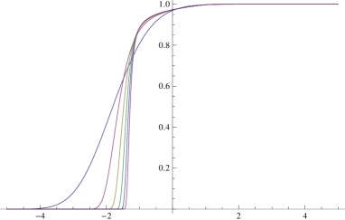
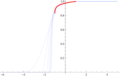
Figure 3: The distributions $F_{k}$ for $k=0,1,\ldots,5$ with $t_{j}=0$. The slope steepens near $-1$ when $k$ increases. On the right, we also plot $F_{\infty}$ (thick curve), as constructed in Section 4.4.

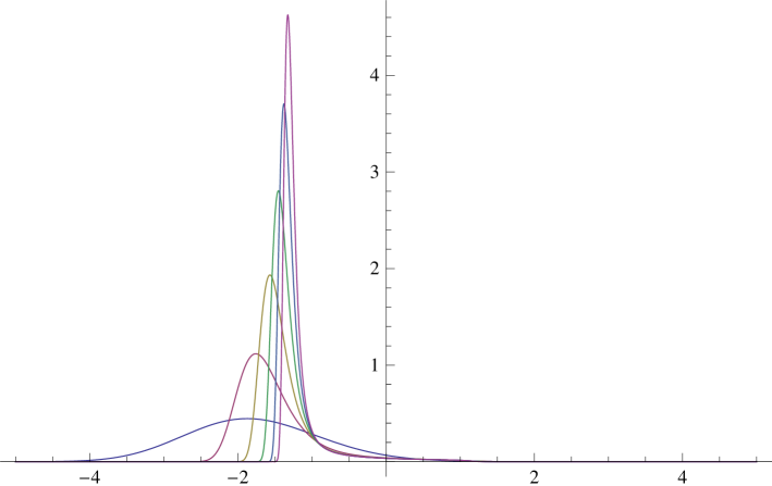
Figure 4: The densities $F_{k}^{\prime}(s)$ for $k=0,1,\ldots,5$ with $t_{j}=0$.

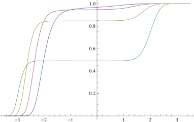
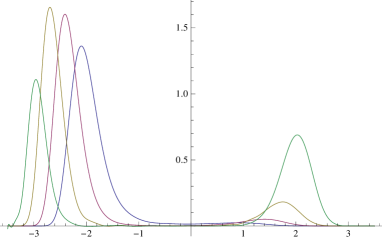
Figure 5: The distribution $F_{1}(s)$ (left) and density $F_{1}^{\prime}(s)$ (right) for $t_{0}=0$ and $t_{1}=-1,\ldots,-4$.

4 Plots and open problems

4.1 Local maxima of the densities

In Figure 3, we plot the numerically computed distributions $F_{k}(s;0,\ldots,0)$ for $k=0,\ldots,5$, where we write

$$F_{k}(s;t_{0},\ldots,t_{2k-1})=\det(I-K_{s}^{(k)}(t_{0},\ldots,t_{2k-1})).$$ (4.1)

In Figure 4 the corresponding densities are drawn. One observes that each of the densities has only one local maximum (i.e. the distributions have only one inflection point). The figures suggest that for any $k\in\mathbb{N}$ and for $t_{0}=\ldots=t_{2k-1}=0$, the densities have only one local maximum.

For general values of the parameters $t_{0},\ldots,t_{2k-1}\in\mathbb{R}$, the situation is different. We see in Figure 5, for $k=1$, $t_{0}=0$ and varying negative $t_{1}$, that the densities have two local maxima. From the random matrix point of view, this can be explained heuristically by the fact that the kernels $K^{(1)}(u,v;0,t_{1})$ for $t_{1}<0$ correspond to a double scaling limit which describes the transition from a random matrix model with a two-cut support (for the limiting mean eigenvalue distribution) to a one-cut support, where the parameter $t_{1}$ regulates the speed of the transition. To be more precise, consider a random matrix ensemble with probability measure (1.1), where $V=V_{n}$ depends on $n$. If the dependence of $V$ on $n$ is fine-tuned in an appropriate way, it can happen that the equilibrium measure $\mu_{V_{n}}$ consists of two intervals for finite $n$, but of only one interval in the limit $n\to\infty$. In order to obtain $K^{(1)}(u,v;0,t_{1})$ as a scaling limit of the eigenvalue correlation kernel, both intervals in the support of $\mu_{V_{n}}$ should approach each other and simultaneously one of the intervals should shrink, as $n\to\infty$. If the $n$-dependence of $V$ is chosen in an appropriate way, the limiting probability that a random matrix has an eigenvalue located in the shrinking interval lies strictly between $0$ and $1$ (it actually increases when $t_{1}$ decreases). We believe that one local maximum of the densities in Figure 5 (the one most to the left) corresponds to the largest eigenvalue if no eigenvalues lie in the shrinking interval, and the second local maximum corresponds to the largest eigenvalue if this one lies in the shrinking interval. For $k\in\mathbb{N}$, transitions can take place from at most $k+1$ cuts to a one-cut regime, and for that reason we expect that for $k\in\mathbb{N}$, the density function has at most $k+1$ local maxima, although we have no analytical evidence for this.

4.2 Asymptotics as $x\to+\infty$

In Figure 6 we show the rate of convergence to one as $s\rightarrow\infty$ of $F_{k}(s)$ for various values of $k$. For $s<1$, we see that the distribution appears to approach a fixed distribution. For $s>1$, the rate of convergence becomes increasingly rapid, matching the asymptotic formula (1.22).

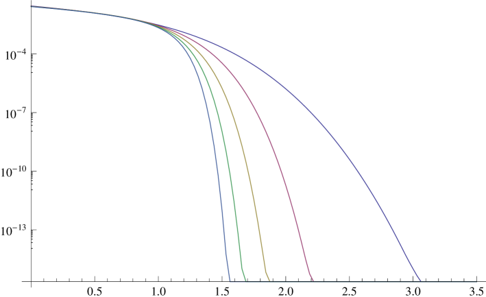
Figure 6: $1-F_{k}(s)$ for $k=1,\ldots,5$ with $t_{j}=0$.

4.3 Asymptotics as $x\to-\infty$

We note that the constants $\chi^{(k)}$ in (1.23) can be expressed as

$$\chi^{(k)} =\lim_{s\rightarrow-\infty}\left(\log\det(I-K_{s}^{(k)})-A_{s}^{(k)}\right)$$

$$=\lim_{s\rightarrow-\infty}\left(\log\det(I-K_{M}^{(k)})-\int_{s}^{M}\partial_{s}\log\det(I-K_{s}^{(k)})ds-A_{s}^{(k)}\right),$$

with

$$A_{s}^{(k)}=-\frac{1}{4(4k+3)}\frac{\Gamma(2k+\frac{3}{2})^{2}}{\Gamma(\frac{3}{2})^{2}\Gamma(2k+2)^{2}}|s|^{4k+3}-\frac{2k+1}{8}\log|s|.$$

For moderate $M$ (we use $M=-.5$), we can reliably calculate $\log\det(I-K_{M}^{(k)})$ as before. For $s<M$, to reliably calculate $\partial_{s}\log\det(I-K_{s}^{(k)})$, we use the RH problem for $R$ used in [5, Section 3.5]. This RH problem is in canonical form and $\partial_{s}\log\det(I-K_{s}^{(k)})$ can be expressed in terms of its solution. We then expand $\partial_{s}\log\det(I-K_{s}^{(k)})-\partial_{s}A_{s}^{(k)}$ in piecewise Chebyshev polynomials, allowing for the efficient calculation of its integral.

To verify the accuracy of the above approach, we need to estimate four errors, which we do using the following heuristics. We estimate the error in calculating $\Psi^{(2k)}$ by ensuring that the smallest computed Chebyshev coefficient is below a given tolerance ($10^{-12}$). The error in $\log\det(I-K_{M}^{(k)})$ is estimated by examining the Cauchy error as the number of quadrature points $m$ in the Fredholm determinant routine increases. The error in $\partial_{s}\log\det(I-K_{s}^{(k)})$ at each point of evaluation $s$ is determined by examining the smallest computed Chebyshev coefficient of the numerical approximation to $R$. Finally, the accuracy of the piecewise Chebyshev approximation to $\partial_{s}\log\det(I-K_{s}^{(k)})$ is estimated by examining each piece’s smallest Chebyshev coefficient.

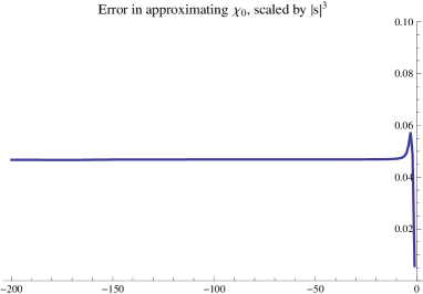
Figure 7: The absolute error in approximating $\chi_{0}$, $|\chi^{(0)}-\log\det(I-K_{s}^{(0)})+A_{s}^{(0)}|$ as a function of $s$ (left). The error multiplied by $|s|^{3}$ (right), showing faster convergence than predicted.

Using this approach, we estimate the first three $\chi^{(k)}$:

$$\chi^{(0)} \approx-0.1365400105,\qquad\hbox{(matches exact expression to 8 digits)}$$

$$\chi^{(1)} \approx-0.09614954\hbox{ and }$$

$$\chi^{(2)} \approx-0.06145.$$

Cancellation and other numerical issues cause the approach to be unreliable for larger $k$.

The convergence to $\chi^{(0)}$ is verified in Figure 7. One interesting thing to note is that the rate of convergence appears to be faster than predicted: numerical evidence suggest convergence like ${\cal O}(|s|^{-3})$. A similar experiment for $\chi^{(1)}$ suggests a convergence rate of ${\cal O}(|s|^{-7})$. (The numerics for $\chi^{(2)}$ are insufficiently accurate to make a prediction.) Therefore, we conjecture that the error term in (1.23) is in fact ${\cal O}(|s|^{-(4k+3)})$, which is better than the theoretical error ${\cal O}(|s|^{-{4k+3\over 2}})$.

4.4 Large $k$ limit

For increasing $k$, one observes from Figure 3 that the slope of the distributions near $-1$ gets steeper. At first sight, one may expect from Figure 3 that for large $k$, the distribution function tends to a step function, but a closer inspection reveals that this is not the case. Instead, we believe that there is a limit distribution supported on $[-1,1]$ which is possibly discontinuous at $-1$ but continuous at $1$.

We present an asymptotic–numerical argument that this is indeed true. Consider the RH problem for $\Psi^{(2k)}$. Note that on $\tilde{\Gamma}_{j}$, the jumps $WS_{j}W^{-1}\rightarrow I$ as $k\rightarrow\infty$. Furthermore, inside the unit circle $W(\zeta)\rightarrow W^{(\infty)}(\zeta)=\zeta^{-\sigma_{3}/4}N$. Finally, $\tilde{\Gamma}_{42}$ disappears. Thus, in a formal sense, we have the following RH problem:

RH problem for $\Psi^{(\infty)}$

• $\Psi=\Psi^{(\infty)}:\mathbb{C}\setminus\Gamma\to\mathbb{C}^{2\times 2}$ is analytic, with

  $$\Gamma =\tilde{\Gamma}_{21}\cup\tilde{\Gamma}_{14}\cup\{\pm 1\},\quad\tilde{\Gamma}_{21}=e^{i\pi(1,0)},\tilde{\Gamma}_{14}=e^{i\pi(0,-1)}.$$

• The jump conditions for $\Psi$ are given by (for $W=W^{(\infty)}$)

  $$\Psi_{+}(\zeta) =\Psi_{-}(\zeta)S_{4}^{-1}W^{-1}(\zeta), \mbox{for $\zeta\in\tilde{\Gamma}_{14}$},$$

  $$\Psi_{+}(\zeta) =\Psi_{-}(\zeta)S_{4}^{-1}S_{1}W^{-1}(\zeta), \mbox{for $\zeta\in\tilde{\Gamma}_{21}$}.$$

• As $\zeta\to\infty$, we have $\lim\Psi(\zeta)=I$.

This is not in canonical form: the jump matrices are not continuous at $\pm 1$, implying that the solution $\Psi^{(\infty)}$ has singularities. We rectify this by using local parametrices to remove the jumps. Define

$$P^{(1)}(\zeta)=\begin{cases}\begin{pmatrix}1&0\\ -1&1\end{pmatrix}\begin{pmatrix}1&{1\over 2\pi i}\log\left(-i{z+i\over z-i}-1\right)\\ 0&1\end{pmatrix}\begin{pmatrix}1&0\\ 1&1\end{pmatrix},&\mbox{$|\zeta-1|<r$, $|z|<1$,}\\ \begin{pmatrix}1&0\\ -1&1\end{pmatrix}\begin{pmatrix}1&{1\over 2\pi i}\log\left(-i{z+i\over z-i}-1\right)\\ 0&1\end{pmatrix}\begin{pmatrix}1&0\\ 1&1\end{pmatrix}S_{3}S_{2}W^{-1},\\ &\mbox{$|\zeta-1|<r$, $|z|>1$,}\end{cases}$$

and

$$P^{(-1)}(\zeta)=\begin{cases}\begin{pmatrix}e^{-2i\pi/3}&e^{2i\pi/3}\\ 1&1\end{pmatrix}\left(-1+i{z+i\over z-i}\right)^{\sigma_{3}/6}\begin{pmatrix}e^{-2i\pi/3}&e^{2i\pi/3}\\ 1&1\end{pmatrix}^{-1},\\ \hskip 227.62204pt\mbox{ for $|\zeta+1|<r$, $|z|<1$,}\\ \begin{pmatrix}e^{-2i\pi/3}&e^{2i\pi/3}\\ 1&1\end{pmatrix}\left(-1+i{z+i\over z-i}\right)^{\sigma_{3}/6}\begin{pmatrix}e^{-2i\pi/3}&e^{2i\pi/3}\\ 1&1\end{pmatrix}^{-1}S_{3}S_{2}W_{+}^{-1},\\ \hskip 227.62204pt\mbox{ for $|\zeta+1|<r$, $|z|>1$,}\end{cases}$$

with the standard branch cuts, so that they lie on the half circle $e^{(0,-i\pi)}$. It is straightforward to verify that $P^{(\pm 1)}$ have the same jumps as $\Psi^{(\infty)}$ inside the disks $|\zeta\mp 1|<r$.

We now define for $r$ sufficiently small,

$$Y(\zeta)=\begin{cases}\Psi^{(\infty)}(\zeta)P^{(1)}(\zeta)^{-1},&|\zeta-1|<r,\\ \Psi^{(\infty)}(\zeta)P^{(-1)}(\zeta)^{-1},&|\zeta+1|<r,\\ \Psi^{(\infty)}(\zeta),&\mbox{otherwise.}\end{cases}$$

Then, $Y$ satisfies a RH problem in canonical form:

RH problem for $Y$

• $Y:\mathbb{C}\setminus\overline{\Delta}\to\mathbb{C}^{2\times 2}$ is analytic, with

  $$\Delta=\Delta_{1}\cup\Delta_{2}\cup\Gamma_{r}(\pm 1)\cup\{\pm e^{\pm i\theta}\},$$

  $$\Delta_{1}=e^{i\pi(1-\theta,\theta)},\quad\Delta_{2}=e^{i\pi(-\theta,\theta-1)},\quad\Gamma_{r}(a)=\{\zeta:|\zeta-a|=r\},$$

  where $\theta$ is given by $r=|e^{i\theta}-1|$.

• The jump conditions for $Y$ are given by

  $$Y_{+}(\zeta) =Y_{-}(\zeta)S_{4}^{-1}S_{1}W^{-1}(\zeta), \mbox{for $\zeta\in\Delta_{1}$},$$

  $$Y_{+}(\zeta) =Y_{-}(\zeta)S_{4}^{-1}W^{-1}(\zeta), \mbox{for $\zeta\in\Delta_{2}$},$$

  $$Y_{+}(\zeta) =Y_{-}(\zeta)P^{(\pm 1)}(\zeta), \mbox{for $\zeta\in\Gamma_{r}(\pm 1)$}.$$

• As $\zeta\to\infty$, we have $\lim Y(\zeta)=I$.

• $Y$ is bounded near $\{\pm e^{\pm i\theta}\}$.

We can compute $Y$, and hence $\Psi^{(\infty)}$ numerically. We therefore define

$$\Phi^{(\infty)}(\zeta)=\Psi^{(\infty)}(\zeta)\begin{cases}0&|\zeta|>1\\ S_{4}^{-1}&|\zeta|<1\hbox{ and ${\rm Im\,}\zeta<0$ }\\ S_{4}^{-1}S_{1}&|\zeta|<1\hbox{ and ${\rm Im\,}\zeta>0$ }\end{cases}.$$

which we use to compute the kernel of $K_{s}^{(\infty)}$, which is a trace-class operator now acting on $L^{2}(s,1)$. (Again, we do not have a rigorous reason why the limiting operator acts only on $L^{2}(s,1)$, not $L^{2}(s,\infty)$. Instead, we justify this by the accuracy of the numerics.)

It should be noted that the local parametrices $P^{(\pm 1)}$ are not close to the identity matrix on $|\zeta\mp 1|=r$, and therefore they would not be suitable parametrices to be used for a rigorous Deift/Zhou steepest descent analysis [12] applied to the RH problem for $\Psi$. However, this is not an issue here: numerically it is sufficient that the local parametrices satisfy the required jump conditions.

While this construction has not been mathematically justified, it is perfectly usable in a numerical way. In fact, the resulting distribution matches the asymptotics for the finite $k$ distributions, cf. Figure 3, providing strong evidence that, for $-1<s<1$,

$$\lim_{k\rightarrow\infty}\det(I-K_{s}^{(k)})=\det(I-K_{s}^{(\infty)}).$$

We remark that the $\Phi^{(\infty)}$ appears to be smooth near $+1$, hence Bornemann’s numerical Fredholm determinant routine remains accurate for $s>-1$. However, the singularity in $\Phi^{(\infty)}$ at $-1$ causes the accuracy to break down as $s$ approaches $-1$. Therefore, we cannot infer whether the distribution approaches zero smoothly, or if there is a jump.

Tom Claeys, tom.claeys@uclouvain.be, Université
Catholique de Louvain, Chemin du cyclotron 2, B-1348
Louvain-La-Neuve, BELGIUM

Sheehan Olver, olver@maths.usyd.edu.au, School of Mathematics and
Statistics, The University of Sydney, NSW 2006 Australia

References

- [1] J. Baik, R. Buckingham, and J. Di Franco, Asymptotics of Tracy–Widom distributions and the total integral of a Painlevé II function, Comm. Math. Phys. 280 (2008), 463–497.
- [2] F. Bornemann, On the numerical evaluation of Fredholm determinants, Math. Comp 79 (2010), 871–915.
- [3] M.J. Bowick and E. Brézin, Universal scaling of the tail of the density of eigenvalues in random matrix models, Phys. Lett. B 268 (1991), no. 1, 21–28.
- [4] E. Brézin, E. Marinari, and G. Parisi, A non-perturbative ambiguity free solution of a string model, Phys. Lett. B 242 (1990), no. 1, 35–38.
- [5] T. Claeys, A. Its, and I. Krasovsky, Higher order analogues of the Tracy–Widom distribution and the Painlevé II hierarchy, Comm. Pure Appl. Math. 63 (2010), 362–412.
- [6] T. Claeys and M. Vanlessen, Universality of a double scaling limit near singular edge points in random matrix models, Comm. Math. Phys. 273 (2007), 499–532 .
- [7] P. Deift, “ Orthogonal Polynomials and Random Matrices: A Riemann–Hilbert Approach”, Courant Lecture Notes 3, New York University 1999.
- [8] P. Deift and D. Gioev, Universality in random matrix theory for the orthogonal and symplectic ensembles, Int. Math. Res. Pap. IMRP 2007 (2007), no. 2, Art. ID rpm004, 116 pp.
- [9] P. Deift, A. Its, and I. Krasovsky, Asymptotics for the Airy-kernel determinant, Comm. Math. Phys. 278 (2008), 643–678.
- [10] P. Deift, T. Kriecherbauer, and K.T–R McLaughlin, New results on the equilibrium measure for logarithmic potentials in the presence of an external field, J. Approx. Theory 95 (1998), 388–475.
- [11] P. Deift, T. Kriecherbauer, K.T–R McLaughlin, S. Venakides, and X. Zhou, Uniform asymptotics for polynomials orthogonal with respect to varying exponential weights and applications to universality questions in random matrix theory, Comm. Pure Appl. Math. 52 (1999), 1335–1425.
- [12] P. Deift and X. Zhou, A steepest descent method for oscillatory Riemann–Hilbert problems. Asymptotics for the MKdV equation, Ann. Math. 137 (1993), no. 2, 295–368.
- [13] S.P. Hastings and J.B. McLeod, A boundary value problem associated with the second Painlevé transcendent and the Korteweg–de Vries equation, Arch. Rational Mech. Anal. 73 (1980), 31–51.
- [14] A.B.J. Kuijlaars and K.T–R McLaughlin, Generic behavior of the density of states in random matrix theory and equilibrium problems in the presence of real analytic external fields, Comm. Pure Appl. Math. 53 (2000), 736–785.
- [15] S. Olver, A general framework for solving Riemann–Hilbert problems numerically, Report no. NA-10/5, Mathematical Institute, Oxford University.
- [16] S. Olver, Numerical solution of Riemann–Hilbert problems: Painlevé II, Found. Comput. Maths 11 (2011), 153–179.
- [17] S. Olver, Computing the Hilbert transform and its inverse, Maths Comp. 80 (2011), 1745–1767.
- [18] M. Prähofer, and H. Spohn, Exact scaling functions for one-dimensional stationary KPZ growth, J. Stat. Phys. 115 (2004), 255–279.
- [19] C.A. Tracy and H. Widom, Level spacing distributions and the Airy kernel, Comm. Math. Phys. 159 (1994), no. 1, 151–174.