Dominant Folding Pathways of a WW Domain

Abstract

We investigate the folding mechanism of the WW domain Fip35 using a realistic atomistic force field by applying the Dominant Reaction Pathways (DRP) approach. We find evidence for the existence of two folding pathways, which differ by the order of formation of the two hairpins. This result is consistent with the analysis of the experimental data on the folding kinetics of WW domains and with the results obtained from large-scale molecular dynamics (MD) simulations of this system. Free-energy calculations performed in two coarse-grained models support the robustness of our results and suggest that the qualitative structure of the dominant paths are mostly shaped by the native interactions. Computing a folding trajectory in atomistic detail only required about one hour on 48 CPU’s. The gain in computational efficiency opens the door to a systematic investigation of the folding pathways of a large number of globular proteins.

Unveiling the mechanism by which proteins fold into their native structure remains one of the fundamental open problems at the interface of contemporary molecular biology, biochemistry and biophysics. A critical point concerns the characterization of the ensemble of reactive trajectories connecting the denatured and native states, in configuration space.

In this context, a fundamental question which has long been debated foldingtheory1 is whether the folding of typical globular proteins involves a few dominant pathways, i.e. well defined and conserved sequences of secondary and tertiary contact formation, or if it can take place through a multitude of qualitatively different routes. A related important question concerns the role of non-native interactions in determining the structure of the folding pathways foldingtheory2 ; foldingtheory3 .

In principle, atomistic MD simulations provide a consistent framework to address these problems from a theoretical perspective. However, due to their high computational cost, MD simulations can presently only be used to investigate the conformational dynamics of relatively small polypeptide chains, and are only able to cover time intervals much smaller than the folding times of typical globular proteins.

In view of these limitations, a considerable amount of theoretical and experimental activity has been devoted to investigate the folding of protein sub-domains, which consist of only a few tens of aminoacids, and fold on sub-millisecond time-scales expfastfolders . In particular, a number of mutants of the 35 aminoacid WW domain of human protein pin1 have been engineered which fold in few tens of microseconds  expWW1 . Their small size and their ultra-fast kinetics make them ideal benchmark systems, for which numerical simulations can be compared with a large body of experimental data expWW1 ; expWW2 ; expWW3 .

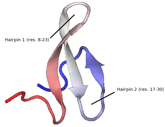
Figure 1: Native structure of Fip35, a WW domain of the fip mutant of protein human pin1 (pdb code: pin1). The primary sequence of fip35 is: EEKLPPGWEKRMSADGRVYYFNHITNASQWERPSG.

In particular, a MD simulation was performed to investigate the dynamics of a mutant named Fip35 (see Fig. 1), for a time interval longer than $10\;\mu$s. Unfortunately, in that simulation no folding transition was observed theWW1 ; theWW2 .

The folding of this WW domain was later investigated by Pande and co-workers, using a world-wide distributed computing scheme  theWW3 . According to this study the transition proceeds in a very heterogeneous way, i.e. through a multitude of qualitatively different and nearly equiprobable folding pathways.

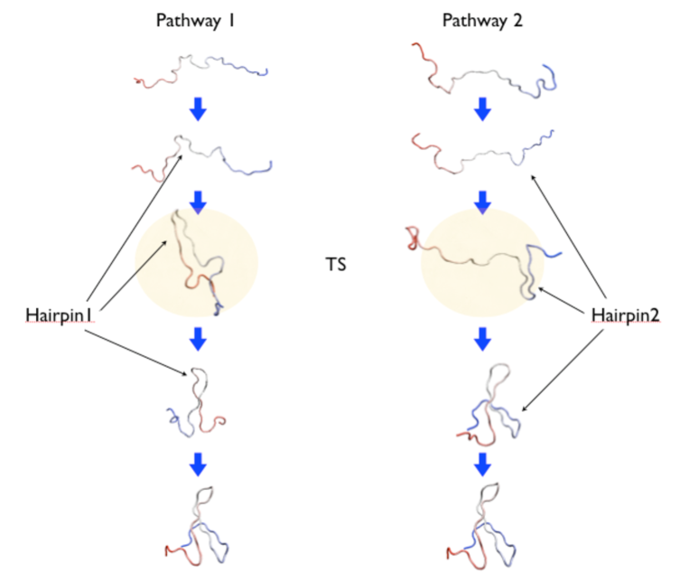
Figure 2: Schematic representation of the structure of the two folding pathways obtained in our DRP simulations.

Noé and co-workers performed a Markov state model analysis of a large number of short ($\lesssim$ 200 ns) nonequilibrium MD trajectories theWW4 performed on the WW domain of human Pin 1 protein. They reported a complex network of transition pathways, which differ by the specific order in which the different local meta-stable states were visited. On the other hand, in all pathways the formation of hairpins takes place in a definite sequence (see e.g. Fig. 2). In particular, from the statistical model it was inferred that in about $30\%$ of the folding transitions, the second hairpin forms first, as in the right panel.

A different conclusion has been reached by Shaw and co-workers, by analyzing a ms-long MD trajectory with multiple unfolding/refolding events, obtained using a special-purpose supercomputer theWW5 . In that simulation the WW domain of Fip35 was found to fold and unfold predominantly along a pathway in which hairpin 1 is fully structured, before hairpin 2 begins to fold, as shown in the left panel of Fig.2. In a recent paper krivov , Krivov re-analyzed the same ms-long MD trajectory in order to identify an optimal set of reaction coordinates. His conclusion was that the folding of this WW domain is thermally activated rather than incipient downhill and that the transition also occurs through a second pathway, in which hairpin 2 forms before hairpin 1. The statistical weights of the two pathways estimated from the number of folding events are $80\%\pm 20\%$ and $20\%\pm 10\%$.

While all these theoretical studies yield folding times in rather good agreement with available experimental data on folding kinetics, they provide different pictures of the folding mechanism and raise a number of issues.

Firstly, it is important to assess the degree of heterogeneity of the folding mechanism and to clarify whether the most statistically significant folding pathways are those in which the hairpins form in sequence. Important related questions are also whether the folding mechanism is correlated with the structure of the initial denatured conditions from which the reaction is initiated and with the temperature of the heat bath. Finally, it is interesting to address the problem of the relative role played by native and non-native interactions in determining the structure of folding pathways. Indeed, while native interactions are arguably shaping the dynamics in the vicinity of the native state, non-native interactions may in principle play an important role in the transition region and at the rate limiting stages of the reaction.

In order to tackle these questions, in this work we use the Dominant Reaction Pathways (DRP) approach DRP1 ; DRP2 ; DRP3 ; DRP4 ; QDRP1 , a framework which allows to very efficiently compute the statistically most significant pathways connecting given denatured configurations to the native state at an atomistic level of detail, with realistic force fields. To further support our results and to study the role of native and non-native interactions we map the free energy landscape by performing Monte Carlo simulations in two coarse-grained models.

Our study confirms that Fip35 folds mostly through the two folding channels discussed above and shows that the relative weight of the two channels changes with temperature. In addition, we find that the folding pathways are correlated with the initial condition from which the transition is initiated. The studies based on the coarse-grained model suggest that the folding dynamics in the transition region is not significantly influenced by non-native interactions.

I Methods

I.1 Atomistic Force Field

Our atomistic simulations of the dominant folding trajectories of the Fip35 WW domain were performed using the AMBER ff99SB force field AMBER99sb in implicit solvent with Generalized Born formalism implemented in GROMACS 4.5.2 GRO4 . The Born radii were calculated according to the Onufriev-Bashford-Case algorithm OBC .

In a recent work based on the DRP method, the dominant pathway in the conformational transition of tetra-alanine obtained using the same version of the AMBER force field was found to agree well with the results of an analogous calculation in which the molecular potential energy was determined ab initio, i.e. directly from quantum electronic structure calculations QDRP2 .

I.2 Coarse-grained Model

To study the equilibrium properties of the folding of the Fip35 WW domain we used the coarse-grained model recently developed in Ref.s Kim&Hummer ; reactioncoord2 . In that model, aminoacids are represented by spherical beads centered at the $C_{\alpha}$ positions. The non-bonded part of the potential energy contains both native and non-native interactions. The former are the same used in the G$\overline{o}$-type model of Ref. Karanikolas&Brooks , while the latter consist of a quasi-chemical potential, which accounts for the statistical propensity of different aminoacids to be found in contact in native structures, and of a Debye-screened electrostatic term. In this model, the average potential energy due to native interactions in the folded phase is typically one order of magnitude larger than that due to non-native interactions. Above the folding temperature, this ratio drops to about 4.

This model was shown to provide an accurate description of protein-protein complexes with low and intermediate binding affinities Kim&Hummer . In the insert of the first panel of Fig. 3 we plot the specific heat, evaluated from MC simulations at different temperatures, which indicates that this model yields the correct folding temperature for this WW domain.

I.3 The Dominant Reaction Pathways Method

The high computational cost of MD simulations of macromolecular systems has triggered efforts towards developing alternative theoretical frameworks to investigate their long-time dynamics and reaction kinetics (see e.g. DRP1 ; method1 ; method2 ; method3 ; method4 ; method5 ; method6 and references therein).

In particular, the DRP approach DRP1 ; DRP2 ; DRP3 ; DRP4 ; QDRP1 ; DRP0 concerns physical systems which can be described by the overdamped Langevin equation. If ${\bf x}_{k}$ denotes the coordinate of the $k-$th atom, the Langevin equation in the so-called Ito Calculus reads:

$${\bf x}_{k}(i+1)={\bf x}_{k}(i)-\frac{\Delta tD_{k}}{k_{B}T}{\bf\nabla}U[{\bf X}(i)]+\sqrt{2D_{k}\Delta t}\,{\bf\eta}_{k}(i).$$ (1)

In this equation, ${\bf X}(i)\equiv({\bf x}_{1}(i),\ldots,{\bf x}_{N}(i))$ is the set of atomic coordinates at the $i-$th time step, $\Delta t$ is an elementary time interval, $D_{k}$ is the diffusion coefficient of the $k-$th atom, $k_{B}$ is the Boltzmann’s constant, $T$ is the temperature of the heat-bath, $U({\bf X})$ is the potential energy. ${\bf\eta}^{k}(i)$ is a white Gaussian noise with unitary variance, acting on the $k-$th atom.

The probability for a protein to fold in a given time interval $t$ can be written as

$$P_{f}(t)=\int d{\bf X}_{f}~{}h_{N}({\bf X}_{f})\int d{\bf X}_{i}~{}h_{D}({\bf X}_{i})~{}P({\bf X}_{f},t|{\bf X}_{i})~{}\rho_{0}({\bf X}_{i}),$$ (2)

where $h_{N(D)}({\bf X})$ is the characteristic function of the native (denatured) state (defined in terms of some suitable order parameters), $\rho_{0}({\bf X}_{i})$ is the initial distribution of micro-states in the denatured state and $P({\bf X}_{f},t|{\bf X}_{i})$ is the conditional probability of reaching the (native) configuration ${\bf X}_{f}$ starting from the (denatured) configuration ${\bf X}_{i}$, in a time $t$. If the total time interval $t$ is chosen much smaller than the inverse folding rate, this probability is dominated by single nonequilibrium folding events.

It can be shown that the probability of a given folding trajectory ${\bf X}(t)$ connecting denatured and native configurations is proportional to the negative exponent of the Onsager-Machlup functional DRP0 ; method5 , which in discretized form reads

$$\text{Prob}[{\bf X}]\propto\exp\left[-\sum_{i=1}^{N_{t}}\sum_{k=1}^{N}\frac{1}{4D_{k}\Delta t}\right.$$

$$\cdot\left.\left({\bf x}^{k}(i+1)-{\bf x}^{k}(i)+\frac{\Delta t~{}D_{k}}{k_{B}T}\nabla U[{\bf X}(i)]\right)^{2}\right],$$ (3)

where $N_{t}$ is the number of time steps in the trajectory. On the other hand, the paths which do not reach native state before time $t$ do not contribute to the transition probability in Eq. 2. The most probable —or so-called dominant— reaction pathways are those which minimize the exponent in Eq. 3. In principle, these may be found by numerically relaxing the effective action functional DRP1 ; Adib

$$S_{eff}[{\bf X}]=\Delta t~{}\sum_{i=1}^{N_{t}}~{}\left[\sum_{k=1}^{N}\frac{({\bf x}_{k}(i+1)-{\bf x}_{k}(i))^{2}}{4D_{k}\Delta t^{2}}+V_{eff}[{\bf X}(i)]\right],$$ (4)

where $V_{eff}({\bf X})$ is the so-called effective potential, and reads

$$V_{eff}({\bf X})=\frac{1}{4(k_{B}T)^{2}}\sum_{k}D_{k}~{}\left(~{}\left|{\bf\nabla}_{k}~{}U({\bf X})\right|^{2}-2~{}k_{B}T\;\nabla_{k}^{2}~{}U({\bf X})\ \right).$$ (5)

In practice, for a protein folding transition, directly minimizing the effective action in Eq. 4 is unfeasible, since at least $10^{4}-10^{5}$ time steps are needed to describe a single folding event. On the other hand, for any fixed pair of native and denatured configurations the dominant paths can be equivalently found by minimizing an effective Hamilton-Jacobi (HJ) action in the form DRP1 ; DRP0

$$S_{HJ}=\sum_{i=1}~{}\Delta l_{i,i+1}\sqrt{\frac{1}{D}\left(E_{eff}+V_{eff}[{\bf X}(i)]\right)},$$ (6)

where and $\Delta l_{i+1,i}=\sqrt{({\bf X}(i+1)-{\bf X}(i))^{2}}$ represents the elementary displacement in configuration space, and for sake of clarity, we have assumed that all atoms have the same diffusion coefficient. The parameter $E_{eff}$ determines the time at which any given frame $l$ of the path is visited:

$$t(l)=\sum_{i\leq l}\Delta l_{i,i+1}~{}\hskip 2.84544pt[4D(E_{eff}+V_{eff}[{\bf X}(i)]~{})]^{-1/2}.$$ (7)

Hence, by adopting the HJ formulation of Eq. 6, it is possible to replace the time discretization with the discretization of the curvilinear abscissa $l$, which measures the Euclidean distance covered in configuration space during the reaction DRP0 . This way, the problem of the decoupling of time scales is bypassed. As a result, only about $10^{2}$ frames are usually sufficient to provide a convergent representation of a trajectory. On the other hand, the HJ formalism requires to perform an optimization in the space of reactive pathways of a functional, which can take complex values, which is in general a complicated task.

The DRP approach displays important similarities with the SDEL (Stochastic Difference Equation in Length) method developed by Elber and co-workers method4 . In particular, while the DRP is based on minimizing the effective HJ action $S_{DRP}=1/\sqrt{D}\int dl\sqrt{V_{eff}[{\bf X}(l)]+E_{eff}}$, in SDEL the folding trajectories are obtained by extremizing the physical HJ action $S_{SDEL}=\int dl\sqrt{U[{\bf X}(l)]-E}$, where $U(x)$ is the potential energy and $E$ is the conserved total mechanical energy.

The SDEL algorithm is presently implemented in the MOIL software for molecular modeling MOIL . In this code, the protein folding trajectories are obtained by means of simulating annealing relaxation, starting from an initial trial trajectory –see e.g. Ref. Elberproteins —. The DRP algorithm is now implemented in DOLOMIT (Dynamics Of muLti-scale mOdels of Molecular transITions), a program under development at the Interdisciplinary Laboratory for Computational Science (Trento). This code uses the MD-based algorithm described in the next section to identify the dominant path.

I.4 Exploration of the Path Space

The reliability of the DRP approach in investigating the protein folding transition crucially depends on the efficiency of the algorithm used to find optimum paths. In the analysis of conformational DRP2 ; QDRP2 or chemical QDRP1 reactions of relatively small molecules, dominant paths can be found by directly optimizing the HJ action in Eq. 6, e.g. using simulated annealing or gradient-based methods. The DRP calculations for protein folding obtained this way have been extensively tested using reduced models in which the relevant degrees of freedom are individual aminoacids and the energy landscape was relatively smooth testDRP1 ; testDRP2 . Unfortunately, when moving from a coarse-grained to an atomistic description, a large amount of frustration is introduced and the energy surface of the model becomes much rougher. Consequently, the relaxation algorithms adopted in our previous calculations were found to provide a poor exploration of the space of folding paths in an all-atom calculation.

In order to overcome this problem, we have used a biased MD algorithm to efficiently produce a large ensemble of paths, starting from a given denatured configuration and reaching the native state ratchetMD2 ; ratchetMD3 ; method3 . In particular, the so-called ratchet-and-pawl MD (rMD) algorithm method3 exploits the spontaneous fluctuations of the system along a specific collective coordinate (CC), towards its native configuration. This is done by introducing a time-dependent bias potential $V_{R}({\bf X},t)$, whose purpose is to make it very unlikely for the system to evolve back to previously visited values of the CC. On the other hand, this bias exerts no work on the system when it spontaneously proceeds towards the native state. We emphasize that this approach is quite different from the one used in steered-MD steeredMD , where an external force is continuously applied to the system, in order to drive it towards the desired state.

Following the work of Ref. method3 we chose a CC $z(t)$, which defines the distance between the contact map in the instantaneous configuration ${\bf X}(t)$ from the contact map in the native configuration ${\bf X}^{\text{native}}$. This way, the energy optimized native configuration has by definition $z=0$. On the other hand, a bias on $z$ does not force nor lock any specific contact, but only imposes a (quasi) monotonic behavior of the total number of native contacts.

In particular, the biasing potential introduced in Ref. method3 is defined as

$$V_{R}({\bf X},t)=\left\{\begin{array}[]{lr r}\frac{k_{R}}{2}(z[{\bf X}(t)]-z_{m}(t))^{2},&\text{for}&\quad z[{\bf X}(t)]>z_{m}(t)\\ 0,&\text{for}&\quad z[{\bf X}(t)]\leq z_{m}(t).\\ \end{array}\right.\vspace{2mm}$$ (10)

In these equations, $z_{m}(t)$ is the minimum value assumed by the collective variable $z$ along the rMD trajectory, up to time $t$.

The value of the collective variable $z$ in the instantaneous configuration $X(t)$ is defined as:

$$z[X(t)]\equiv\sum_{i,j}^{N}[C_{ij}[{\bf X}(t)]-C_{ij}({\bf X}^{\text{native}})]^{2}.$$ (11)

The entries of the contact map C_ij are chosen to interpolate smoothly between 0 and 1, depending on the relative distance of the residues $i$ and $j$:

$$C_{ij}({\bf X})=\frac{1-(\frac{r_{ij}}{r_{0}})^{6}}{1-(\frac{r_{ij}}{r_{0}})^{10}},$$ (12)

where r₀=7.5 Å  is a fixed reference distance. The variable $z_{m}$(t) is updated only when the system visits a configuration with a smaller value of the CC, i.e. any time $z[{\bf X}(t+\delta t)]<z_{m}(t)$.

The value of the spring constant $k_{R}$ in the ratchet potential —see Eq. 10— controls the amount of bias introduced by the ratchet algorithm. At very low values of $k_{R}$, the rMD trajectories are minimally biased. However, in this limit the system performs the first folding transition on typical time intervals comparable with the folding time $t\sim 1/k_{f}$ —where $k_{f}$ is the folding rate—. On the other hand, the DRP method is based on the transition probability given Eq. 2, where the time interval $t$ is of the order of the transition path time $t_{TPT}\ll 1/k_{f}$. Hence, DRP simulations based on ratchet simulations in which $k_{R}$ is chosen too small are computationally very expensive, since most paths do not reach the native state within the time interval $t$ entering Eq. 2, hence do not contribute to the transition probability.

In the opposite high $k_{R}$ limit, the bias force becomes comparable with the physical internal forces acting on the atoms and the dynamics is affected by a significant bias. In this regime, if the ratcheting coordinate is not optimal, the system is driven into relatively large free energy regions. The unbiased statistical weight given by Eq. 3 penalizes these trajectories. In the extremely high $k_{R}$ limit, the bias towards forming native contacts is very large, and breaking a native contact which is present in a (partially) misfolded configuration becomes extremely unlikely. As a result, also rMD simulations in which $k_{R}$ is chosen too large have a low folding yield, since the trajectories have a large probability to be trapped in misfolded states.

This algorithm allows to efficiently generate a large number of trajectories starting from the same configuration and reaching the native state, hence it can be used to explore the folding path space. Eq. 3 provides a rigorous way to score such trial trajectories, i.e. to evaluate the probability for each of them to be realized in an unbiased overdamped Langevin dynamics simulation. In particular, the best estimate for the dominant folding pathway is the one with the smallest Onsager-Machlup action. The path may then be used as a starting point for a further refinement based on a local relaxation of the HJ action given by Eq. 6, performed by means of the optimization algorithms described in our previous work (see e.g. Ref. QDRP2 ; QDRP3 ).

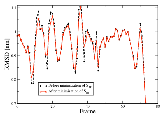
Figure 4: The effect of the minimization of the HJ functional 6 on a trial path obtained from the rMD algorithm on the RMSD to native of the $C_{\alpha}$ atoms in the backbone. This second refinement step does not change the qualitative structure of the dynamics.

The second refinement step is computationally very expensive, requiring several thousands of CPU hours for each dominant trajectory. However, by performing a number of test simulations, we have found that it produces only very small rearrangements of the chain, mostly filtering out small thermal fluctuations (see e.g. Fig.4).

Some comments on the minimization procedure described above are in order: first, we emphasize that since the dynamics generated by the rMD algorithm has infinite memory, it violates the detailed-balance condition and the time intervals computed from the biased trajectories have no direct physical meaning. On the other hand, once a minimum of the HJ action has been identified, it is in principle possible to reconstruct the physical time at which each frame is visited, by means of Eq. 7.

As long as one is concerned mostly with the global qualitative aspects of the folding mechanism, the expensive refinement session of the DRP calculation may be dropped. This allows us to reduce the total computational time required to perform the analysis by several orders of magnitude. On the other hand, we are not in a condition to provide a reliable estimate of the time interval that the protein takes to complete a folding reaction.

We stress that the present DRP approach is expected to give unreliable results if the sampling of the trial trajectories is too limited or if the CC adopted in the bias potential of the rMD algorithm was a bad reaction coordinate. A number of recent studies have shown that the total number of native contacts represents reasonable reaction coordinate for the folding of small globular proteins  reactioncoord2 ; reactioncoord1 ; reactioncoord3 .

Table 1: Summary of the simulation details

Unfold. MD steps	Therm. MD steps	Fold. rMD steps	Denatured	Rejected
(T= 1600 K)	(T= 300 K)	(T= 300 K)	initial conditions
$50\times 10^{3}$	$100\times 10^{3}$	$50\times 10^{3}$	44	18

I.5 Computational Procedures and Simulation Details

The atomistic DRP calculations were performed using DOLOMIT. The code calls a librarized version of GROMACS 4.5.2 GRO4 to calculate the molecular potential energy and its gradient.

We defined the native state as the set of conformations with a RMSD to the crystal structure of the $C_{\alpha}$ in the hairpins smaller than 3.5 Å. A configuration was considered denatured if the RMSD to native of both hairpins was larger than 6Å. The stability of the native state within the present force field was checked by running 12 unbiased 2 ns-long MD simulations at the room temperature (300 K). In all such trajectories the protein remained in the native state. We then generated 44 independent initial conditions, by running a 50 ps MD at 1600 K, starting from the energy minimized native state, followed by a 100 ps relaxation at 300 K. The time step employed in all the simulations was 1 fs. From each of the 24 starting configurations we performed 96 independent runs, each consisting of 50000 rMD steps. For each of the remaining 20 initial conditions, the number of trial paths was limited to 48.

In our simulations, we have chosen the ratchet spring constant $k_{R}=0.02$ kcal/mol, which represents a reasonable compromise between keeping a high computational efficiency for the path exploration and introducing a small bias. Indeed, using this value, the modulus of the biasing force is always at least one order of magnitude smaller than the norm of internal forces.

We observed that 5 of the 44 initial conditions did not correspond to denatured states, hence they were rejected. In addition, in 13 of the remaining 39 sets, more than $80\%$ of the trial trajectories did not reach the native state within the simulation time. In these cases the exploration of the path space was limited to very few trial trajectories, so the corresponding dominant paths were discarded. For the remaining 26 sets of paths, we identified the most probable by computing the OM action of Eq. 3. The complete set of atomistic simulations required less than two days of calculation on 48 CPU’s.

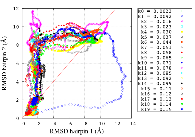
Figure 5: Dominant pathways obtained with different values of the ratchet force, starting from the same initial condition. The values of $k_{R}$ are given in units of kcal/mol.

It is important to study to what extent DRP results obtained this way depend on the value of the bias constant $k_{R}$ adopted in the rMD simulations. In Fig. 5 we plot the dominant reaction pathway obtained starting from the same initial condition, using different values of $k_{R}$ which span over almost two orders of magnitude. We see that in most simulations the folding occurs through the same qualitative pathway, in which the first hairpin forms before the second begins to fold. Only in one case —for a low value of the coupling constant $k_{R}$— we find that the protein travels across the denatured state before taking a different pathway to the native state, in which the order of formation of the hairpins is reversed. Such a trajectory spends a much longer fraction of rMD steps in exploring the denatured state and initiates the transition from a very different configuration.

It is interesting to note that the most probable path turns out not to be the one with the lowest ratchet constant. In particular, the trajectory taking the second pathway (labelled with $K_{1}$ in Fig. 5) is among those with the lowest statistical weight. This is because the OM action tends to penalize paths which travel long Euclidean distances in configuration space. This result illustrates that choosing a low ratchet constant $k_{R}$ produces an enhanced exploration of the denatured state, but does not necessarily lead to a more efficient identification of the most probable trajectories connecting given boundary condition at fixed times.

Once a dominant path has been found, it is relatively straightforward to identify the configuration which belongs to the transition state ensemble. This can be done by finding the frame ${\bf X}_{TS}$ in the trajectory such that the probability to reach the native state is equal to that of going back to the denatured configuration DRP2 :

$$\frac{\text{Prob}[{\bf X}_{TS}\to\text{Unfolded}]}{\text{Prob}[{\bf X}_{TS}\to\text{Native}]}\simeq\frac{e^{-S_{OM}({\bf X}_{TS}\to{\bf X}_{D})}}{e^{-S_{OM}({\bf X}_{TS}\to{\bf X}_{N})}}=1$$ (13)

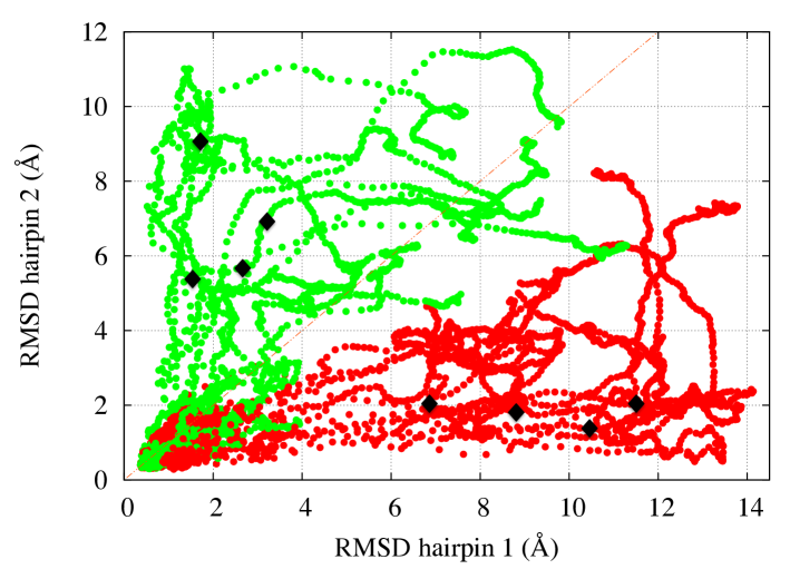
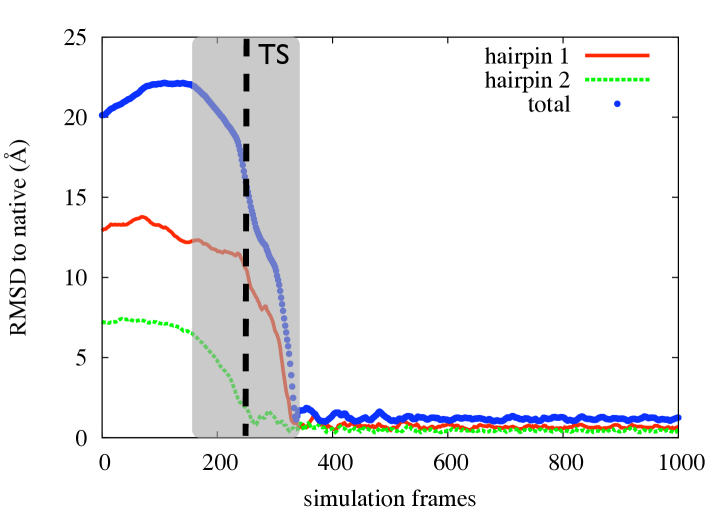
Figure 6: Upper panel: the set of dominant folding paths for Fip35, obtained from atomistic DRP simulations, projected on the plane defined by the RMSD of the two hairpins to the corresponding native structures. The dark spots represent a few typical configurations in the two transition states, evaluated by the requesting a probability 1/2 to reach the native state. Lower panel: evolution of the RMSD to native of the full protein and of the hairpins along a dominant trajectory. The shaded area is the reactive region and the dashed line identifies the transition state configuration obtained according to Eq. 13.

In this equation ${\bf X}_{N}$ and ${\bf X}_{D}$ are the first native and denatured configurations visited along the dominant path, starting from ${\bf X}_{TS}$. In order to locate them, we need to only take into account the “reactive” part of the path, that is the one which leaves the denatured state and, without recrossing, goes straight to the native. To satisfy this requirement, we considered the total RMSD versus frame index curve. The typical trend of this curve for most of the dominant trajectories is shown in the lower panel of Fig. 6: it consists in an initial plateau, followed by a rather steep fall, and then by another flat region, where the system oscillates in the native state. The reactive part of the path was identified with the region of steep fall in this curve. In particular, the beginning of the transition was set to the frame at which the derivative of the total RMSD curve changes sign, from positive to negative.

The simulations of the equilibrium properties of the WW-domain in the coarse-grained models were performed using a Monte Carlo algorithm based on a combination of Cartesian, crankshaft crankshaftMC and pivot pivot moves. The free energy as a function of an arbitrary set of reaction coordinates (potential of mean force) was obtained from the frequency histogram calculated from long MC trajectories.

II Results and Discussion

In the upper panel of Fig.6 we show our set of atomistic dominant folding trajectories, projected onto the plane defined by the RMSD to the native structure of the C_α atoms in residues $8-23$ (hairpin 1) and $17-30$ (hairpin 2).

Two distinct folding pathways which differ by the order of formation of the hairpins can be clearly identified: in about half of the computed dominant folding pathways hairpin 1 consistently folds before hairpin 2. In this channel, we find the transition state is located at the “turn" of the paths, i.e. is formed by configurations in which the hairpin 1 is folded while hairpin 2 is largely unstructured (see pathway 1 in Fig. 2). This is the mechanism predominantly found in the simulation of Ref. theWW5 , performed using the same force field, albeit in explicit solvent.

In about half of the computed dominant paths, we observe that the two hairpins form in the reversed order. In this channel, the transition state is formed by the configurations in which hairpin 2 is folded, while hairpin 1 is unstructured (see pathway 2 in Fig. 2).

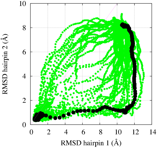
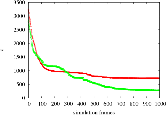
Figure 7: Upper panel: The set of trial paths connecting a given denatured configuration to the native state, used in the search for the dominant paths, projected on the plane defined by the RMSD to native of the two hairpins. The darker path is the selected dominant reaction pathways. Lower panel: the evolution of the biasing coordinate, in two typical folding trajectories of this set.

An important point to emphasize is that this clean two-channel folding mechanism is a prediction of the DRP approach which could not be obtained if we analyzed directly the full set of (biased) trajectories obtained from the rMD algorithm, without scoring their probability. For example, Fig. 7 shows that not all the rMD trajectories computed starting from a given initial condition follow one of the two folding pathways discussed above. Indeed, many of them involve a simultaneous formation of native contacts in both hairpins. A clear prediction of the DRP formalism is that folding events in which the hairpins form simultaneously are much less frequent than those in which the two secondary structures forms in sequence.

Another result emerging from our DRP calculation is the existence of a correlation between the structure of the initial conditions from which the transition is initiated and the pathway taken to fold: if at the beginning of the transition the first hairpin has a RMSD smaller than the second hairpin, then the first pathway is most likely chosen. In the opposite case, i.e. when the second hairpin has a smaller RMSD to native than the first, then the second pathway is generally preferred.

In order to further support these results and gain insight into the folding mechanism, we have performed simulations in an entirely different approach, i.e. by computing equilibrium properties using the coarse-grained models described in the Methods section. In Fig. 3 we show the free energy landscape at the 300 K, as a function of the RMSD to native of the two hairpins for the two models, which differ by the presence of non-native interactions. In both cases, we observe the existence of two valleys in the free energy landscape, which correspond to the two folding pathways discussed above. Remarkably, the same structure for this free energy map was obtained by Ferrara and co-workers for the 20-residue peptide beta3s —which shares the same native topology of WW domains ferrara — by means of equilibrium atomistic simulations based on the CHARMM force field, in implicit solvent.

We emphasize that this set of qualitatively consistent results has been obtained using different algorithms (in equilibrium and nonequilibrium conditions) and different theoretical models (atomistic and coarse-grained). The fact that models with and without non-native interactions give very similar free energy landscapes suggests that the structure of the two folding pathways of WW domains is mostly shaped by native interactions.

II.1 Comparison with experimental data on folding kinetics

In general, all experimental data on folding kinetics of WW domains indicate that the formation of the first hairpin is the main rate limiting step expWW1 ; expWW2 ; expWW3 . In particular, the $\phi$-values measured by Jäger and co-workers display a clear peak in the region associated with hairpin 1, but significant $\phi$–values were reported also for residues in the sequence region relative to hairpin 2 expWW3 . This fact indicates that the folding of the latter structure has some rate limiting effect. In addition, it was found that the $\phi$–values in the region of the second hairpin grow with temperature, while those in the region of the first hairpin decrease. This implies that, at higher and higher temperatures, the second hairpin plays an increasing role in the folding mechanism.

An analysis based on $\phi-$values alone does not permit to fully characterize the folding mechanism. In particular, it cannot distinguish between a single-channel folding mechanism in which native contacts in the two hairpins form simultaneously and a multiple-channel folding mechanism in which the reaction rate in each channel is limited by the folding of one of the hairpins. In Ref. weikl Weikl has shown that the full body of existing $\phi$–value data (taken from Ref.s expWW2 ; expWW3 ) can be consistently and quantitatively explained by a simple kinetic model in which the folding of WW domains occurs through alternative channels, which correspond to the two pathways found in our DRP simulations. From a global fit of the experimental data, the author concluded that the relative probability of the first folding pathway for FBP and Pin 1 WW domain are $77\%\pm 5\%$ and $67\pm 5\%$, respectively.

Let us now discuss the relative statistical weight of the two folding pathways. To this goal we need to estimate and compare the reaction rates in the two channels. The formalism for evaluating reaction rates in the DRP approach was developed in detail in Ref. DRP4 , where it was shown that this method reproduces Kramers theory in the low-temperature regime. Applying that formalism, the ratio of the folding rates in the two channels reads

$$\frac{k_{1}}{k_{2}}\simeq\frac{\kappa^{1}_{0}}{\kappa^{2}_{0}}~{}e^{-\beta~{}(G_{TS_{1}}-G_{TS_{2}})},$$ (14)

where the label 1 (2) identifies the channel in which hairpin 1 (2) folds first. In Eq. 14, the exponent contains the difference of the free-energies of the two transition states, defined from the dominant trajectories according to the commitment analysis described in the Methods section and in Ref.  DRP2 . In particular, one has

$$e^{-\beta G(TS_{i})}\equiv\int d{\bf X}~{}e^{-\beta U({\bf X})}\delta\left[({\bf X}-{\bf X}_{TS}^{i})\cdot\hat{n}_{TS^{i}}\right]\qquad(i=1,2),$$ (15)

where ${\bf X}^{i}_{TS}$ is a point of the transition state which is visited by a typical dominant path in the $i-$th reaction channel and $\hat{n}_{TS^{i}}$ is a versor tangent to the dominant path at ${\bf X}_{TS}^{i}$. Using Eq. 13 to identify the transition states, we have found that the two partition functions defined in Eq. 15 are dominated by configurations in which one of the hairpin is fully formed while the other is still completely unstructured (see Fig. 6). The average location of the computed transition states in the plane defined by the RMSD to native of the two hairpins is highlighted in the lower panel of Fig. 3 and can be identified with the endpoints of the two low free energy valleys.

The coefficients $\kappa_{0}^{1}$ and $\kappa_{0}^{2}$ in the prefactor of Eq. 14 are defined in terms of quantities which can be calculated from the dominant paths — see Ref.DRP4 for details—. These terms estimate the average flux of reactive trajectories across the iso-committor dividing surface, including the contributions from small thermal fluctuations around the dominant paths. Unfortunately, evaluating $\kappa_{0}^{1}$ and $\kappa_{0}^{2}$ necessarily requires to perform the computationally expensive local optimization of the HJ action. However, if the reaction is thermally activated, the ratio of rates $k_{1}/k_{2}$ is mostly controlled by the exponential contribution. Hence, we can consider the Arrhenius approximation

$$\frac{k_{1}}{k_{2}}\simeq e^{-\beta~{}(G_{TS_{1}}-G_{TS_{2}})}.$$ (16)

We emphasize that in this approach the DRP information about the nonequilibrium reactive dynamics is used to define the two transition states. On the other hand, the numerical value of the free energy difference may be obtained from equilibrium techniques, e.g. by sampling the integrals in Eq. 15 by means of computationally very expensive umbrella sampling or meta-dynamics Metadinamica atomistic calculations.

In this first exploratory application of the DRP formalism to a realistic protein folding reaction we choose to perform a much rougher estimate which relies on two main approximations. First, we identify the difference $(G_{TS_{1}}-G_{TS_{2}})$ in Eq. 16 with the difference of the free energy in the two shaded regions of the energy landscape shown in Fig. 3. The centers of these regions represent the average location of the configurations in the two transition states TS1 and TS2 obtained from DRP simulations, projected onto the plane selected by the RMSD to native of the two hairpins. The sizes of the shaded area represents the errors on the average location of the transition states on this plane, estimated from the standard deviation. The second assumption of our model is that such a free energy difference is driven by the balance between energy gain and entropy loss associated to the formation of native contacts in the two hairpins. This native-centric standpoint is supported in part by the fact that free energy landscapes computed in different models with and without non-native interactions are found to be very similar, as it is clear from comparing the panels in Fig. 3. Hence, to estimate $G_{TS_{1}}-G_{TS_{2}}$ we used the G$\overline{o}$-type model described in the Methods section. It is important to emphasize that we are not computing the rate directly from a transition state theory formulated in the coarse-grained model, but we are using it only to estimate a free energy difference.

This way, we obtained an estimate $k_{1}/k_{2}\simeq 2.3$ which corresponds to a relative weight of the first folding channel of $70\%$ and $30\%$. We stress that, such a simple calculation should be considered only a rough estimate. It indicates that the two channels have more or less comparable weight and that the first channel is the most probable, in qualitative agreement with experimental results and with the simulations of Shaw and co-workers.

This simple scheme enables us to address the question of the dependence of the relative weights of the two channels on the temperature. Repeating the calculation at a higher temperature of $380$ K — assuming that the structure of the transition states is not significantly modified— we find $k_{1}/k_{2}\simeq 1.6$, which corresponds to a branching ratio of channel 1 of about $60\%$. Hence, the rate limiting role of the second channel grows with temperature, in qualitative agreement with experimental kinetic data.

This fact can be understood as follows. The folding of one of the hairpins generates an entropy loss proportional to the number $n$ of native contacts formed. More precisely, assuming that the protein in the unfolded state is completely denatured then the entropy loss in the TS of the first (second) channel is $\Delta S_{TS1(TS2)}=n_{1}(n_{2})s$, where $s$ is the entropy loss for locking one residue in its native conformation, while $n_{1}=15$ and $n_{2}=13$ are the numbers of residues in the two hairpins of Fip35. The transition state in the first channel involves forming a longer hairpin, hence reaching it involves a larger entropy loss (but also larger gain of native energy). The role of the entropy loss relative to the energy gain in forming the hairpins grows with temperature, hence disfavoring the first folding channel relative to the second.

III Conclusions

In this work we have studied the folding mechanism of the WW domain Fip35 in equilibrium and nonequilibrium conditions, using an atomistically detailed force field and coarse-grained models based on knowledge-based potentials.

The obtained folding trajectories are not heterogeneous, but rather suggest that the folding proceeds through two dominant channels, defined by a hierarchical order of hairpin formation. In the most probable channel at room temperature, the first hairpin is almost fully formed before the second hairpin starts to fold. In the alternative route, the order of hairpin formation is reversed. Our simulations also suggest that the choice of the folding pathway is correlated with the structure of the denatured configuration from which the peptide initiates the folding reaction. Our results are compatible with both Weikl’s analysis of kinetic data and Krivov’s analysis of equilibrium MD simulations.

The most important result of this work is to show that, using the DRP approach, it is possible to characterize at least the main qualitative aspects of the folding mechanism at an extremely modest computational cost, in the range of few hundreds of CPU hours. Such a level of computational efficiency opens the door to the investigation of the folding pathways of a large number of single-domain proteins, with sizes significantly larger than that of the small domain studied in the present work.

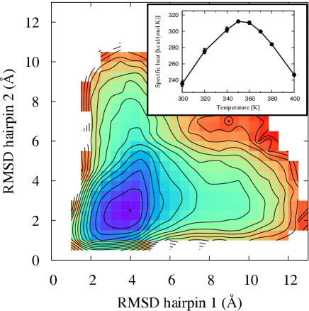
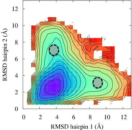
Figure 3: The free energy at $T=300K$ as a function of the RMSD to native of the two hairpins, obtained from the Monte Carlo simulations in two coarse-grained models, described in the Method section. In the upper panel the model accounts for both native and non-native interaction, in the lower panel the model contains only native interactions. In the insert of the upper panel, we show the corresponding plot of the specific heat. Both models predict the existence of two distinct folding paths. The two shaded regions in the lower panel, with coordinates in the range (3.5 $\pm$ 0.5 Å, 7 $\pm$ 0.5 Å) and (9$\pm$ 0.5 Å, = 3.0 $\pm$ 0.5 Å) are identified with the average location of the transition states obtained with DRP simulations. The average of the free energy in these region are used to estimate the relative rate of the two reaction channels.

- (1) Snow, C.D., Sorin, E.J., Rhee, Y.M., & Pande, V.S., (2005) Annual review of biophysics and biomolecular structure 34, 43–69.
- (2) Mirny, L. & Shakhnovich, E., (2001) Annual review of biophysics and biomolecular structure 30, 361–96.
- (3) Onuchic, J.N. & Wolynes, P.G., (2004) Current opinion in structural biology 14(1), 70–5.
- (4) Kubelka, J., Hofrichter, J., & Eaton, W., (2004) Current opinion in structural biology 14(1), 76–88.
- (5) Liu, F., Du, D., Fuller, A., Davoren, J.E., Wipf, P., Kelly, J.W., & Gruebele, M., (2008) Proceedings of the National Academy of Sciences of the United States of America 105(7), 2369–74.
- (6) Deechongkit, S., Nguyen, H., Powers, E.T., Dawson, P.E., Gruebele, M., & Kelly, J.W., (2004) Nature 430(6995), 101–5.
- (7) Jäger, M., Nguyen, H., Crane, J.C., Kelly, J.W., & Gruebele, M., (2001) Journal of molecular biology 311(2), 373–93.
- (8) Freddolino, P.L., Liu, F., Gruebele, M., & Schulten, K., (2008) Biophysical journal 94(10), L75–7.
- (9) Freddolino, P.L., Park, S., Roux, B., & Schulten, K., (2009) Biophysical journal 96(9), 3772–80.
- (10) Ensign, D.L. & Pande, V.S., (2009) Biophysical journal 96(8), L53–5.
- (11) Noé, F., Schütte, C., Vanden-Eijnden, E., Reich, L., & Weikl, T.R., (2009) Proceedings of the National Academy of Sciences of the United States of America 106(45), 19011–6.
- (12) Shaw, D.E., Maragakis, P., Lindorff-Larsen, K., Piana, S., Dror, R.O., Eastwood, M.P., Bank, J., Jumper, J.M., Salmon, J.K., Shan, Y., & Wriggers, W., (2010) Science (New York, N.Y.) 330(6002), 341–6.
- (13) Piana, S., Lindorff-Larsen, K., & Shaw, D.E., (2011) Biophysical journal 100(9), L47–9.
- (14) Faccioli, P., Sega, M., Pederiva, F., & Orland, H. (2006) Physical Review Letters 97(10), 1–4.
- (15) Sega, M., Faccioli, P., Pederiva, F., Garberoglio, G., & Orland, H. (2007) Physical Review Letters 99(11), 1–4.
- (16) Autieri, E., Faccioli, P., Sega, M., Pederiva, F., & Orland, H., (2009) The Journal of chemical physics 130(6), 064106.
- (17) Mazzola, G., a Beccara, S., Faccioli, P., & Orland, H., (2011) The Journal of chemical physics 134(16), 164109.
- (18) a Beccara, S., Garberoglio, G., Faccioli, P., & Pederiva, F., (2010) The Journal of chemical physics 132(11), 111102.
- (19) Wang, J., Cieplak, P., & Kollman, P.A., (2000) Journal of Computational Chemistry 21(12), 1049.
- (20) Hess, B., Kutzner, C., van derSpoel, D., & Lindahl, E., (2008) Journal of Chemical Theory and Computation 4(3), 435–447.
- (21) Onufriev, A., Case, D., &Bashford. D., (2004) Proteins 55, 383–394.
- (22) a Beccara, S., Faccioli, P., Sega, M., Pederiva, F., Garberoglio, G., & Orland, H., (2011) The Journal of chemical physics 134(2), 024501.
- (23) Kim, Y.C. & Hummer, G., (2008) Journal of molecular biology 375(5), 1416–33.
- (24) Best, R.B. & Hummer, G., (2005) Proceedings of the National Academy of Sciences of the United States of America 102(19), 6732–7.
- (25) Karanicolas, J., & Brooks III, C.L., (2002) Protein Science 11(10), 2351–2361.
- (26) Dellago, C., and Bolhuis, P.G. and Geissler, P.L., (2002) Transition Path Sampling (John Wiley & Sons, Inc., Hoboken, NJ, USA), Vol 123.
- (27) Chodera, J.D., Swope, W.C., Pitera, J.W., & Dill, K., (2006) Multiscale Modeling & Simulation 5(4), 1214.
- (28) Camilloni, C., Broglia, R.A., & Tiana, G., (2011) The Journal of chemical physics 134(4), 045105.
- (29) Paci, E. & Karplus, M. (1999) Journal of Molecular Biology 288, 441–459.
- (30) Ghosh, A., Elber, R., & Scheraga, H., (2002) Proceedings of the National Academy of Sciences of the United States of America 99(16), 10394–8.
- (31) Eastman, P., Gronbech-Jensen, N., & Doniach, S., (2001) The Journal of Chemical Physics 114(8), 3823.
- (32) Dryga, A., & Warshel, A., (2010) The journal of physical chemistry. B 114(39), 12720–8.
- (33) Elber, R., & Shalloway, D., (2000) The Journal of Chemical Physics 112(13), 5539.
- (34) Faccioli, P., (2010) The Journal of chemical physics 133(16), 164106.
- (35) Chung, H.S., Louis J. M and Eaton, W. A., (2009) Proceedings of the National Academy of Sciences of the United States of America 106(29), 11837–11844.
- (36) Adib, A.B., (2008) The journal of physical chemistry. B 112(19), 5910–6.
- (37) Faccioli, P., (2008) The journal of physical chemistry. B 112(44), 13756–64.
- (38) Faccioli, P., Lonardi, A., & Orland, H., (2010) The Journal of chemical physics 133(4), 045104.
- (39) Elber, R, Roitberg A., Simmerling C., Goldstein R., Li, H., Verkhivker, G, Keasar C. , Zhang J., & Ulitsky, A. (1995) Computer Physics Communication 91, 159–189.
- (40) Cardenas, E & Elber, R. (2003) Proteins 51, 245–257.
- (41) Marchi, M., & Ballone, P., (1999) The Journal of Chemical Physics 110(8), 3697.
- (42) Zuckerman, D.M., & Woolf, T.B., (1999) The Journal of Chemical Physics 111(21), 9475.
- (43) Isralewitz, B., Gao, M., & Schulten, K., (2001) Current opinion in structural biology 11(2), 224–30.
- (44) a Beccara, S., Garberoglio, G., & Faccioli, P., (2010) The Journal of chemical physics pp. 1–12.
- (45) Best, R.B., & Hummer, G., (2006) Physical review letters 96(22), 228104.
- (46) Cho, S.S., Levy, Y., & Wolynes, P.G., (2006) Proceedings of the National Academy of Sciences of the United States of America 103(3), 586–91.
- (47) Kremer, K., & Binder, K., (1988) Computer Physics Reports 7(6), 259–310.
- (48) Madras, N., & Sokal, A.D., (1988) Journal of Statistical Physics1-2(50), 109–186
- (49) Weikl, T.R., (2008) Biophysical Journal 94, 929–937
- (50) Krivov, S.V., (2011) Journal of Physical Chemistry B 2011, 115 (42), pp 12315–12324
- (51) Ferrara, P., & Caflish, A., (2000) Proceedings of the National Academy of Sciences of the United States of America 97, (20) 10780–10785.
- (52) Laio, A. and Parrinello, M. (2002), Proceedings of the National Academy of Sciences of the United States of America 99, (20) 12562–12566.