Polygons of the Lorentzian plane and spherical simplexes

1 Introduction

It is a common occurence that sets of geometric objects themselves carry some kind of geometric structure. A classical example for this is the set of all conformal structures on a given compact surface. Riemann discovered that this set, the “space” of conformal structures, can be described by a finite number of parameters called moduli. The corresponding parameter or moduli space turned out to be a very interesting geometric object in itself whose study is the subject of Teichmüller theory.

On a more basic level, one can consider spaces consisting of objects of elementary geometry like (shapes of) polyhedra in Euclidean space. Thurston [Thu98] found that in this case, the corresponding moduli space carries the structure of a complex hyperbolic manifold, and he established a link with sets of triangulations of the 2-sphere.

Bavard and Ghys [BG92] considered sets of polygons in the Euclidean plane. Fix a compact convex polygon $P$ with $n\geq 3$ edges and let ${\cal P}(P)$ be the space of convex polygons with $n$ edges parallel to those of $P$. The elements of ${\cal P}(P)$ are then determined by the distances of the lines containing the edges from the origin, which gives $n$ parameters. Following [Thu98], Bavard and Ghys proved that on the space of parameters, the area of the polygons in ${\cal P}(P)$ is a quadratic form, and they computed its signature. The kernel of the corresponding bilinear form has dimension 2 (due to the fact that area is invariant under translations), and there is only one positive direction. Hence, up to the kernel, one gets a Lorentzian signature. As a consequence, the set of elements of ${\cal P}(P)$ with area equal to one, considered up to translations, can be identified with a subset of the hyperbolic space $\mathbb{H}^{n-3}$. This subset turns out to be a hyperbolic convex polyhedron of a special kind: it is a simplex with the property that each hyperplane containing a facet meets orthogonally all but two hyperplanes containing the other facets. Such simplices are called hyperbolic orthoschemes. The dihedral angles of the orthoscheme can be computed from the angles of $P$, and [BG92] contains a list of convex polygons $P$ such that the orthoscheme obtained from $P$ is of Coxeter type, i.e. has acute angles of the form $\pi/k$, $k\in\mathbb{N}$. This list was previously known [IH85, IH90], but it appeared it was incomplete [Fil11].

In this paper we consider a class of non-compact plane polygons whose moduli space is a spherical orthoscheme. These polygons, the $t$-convex polygons introduced in Section 3, are best described not in terms of the Euclidean geometry on $\mathbb{R}^{2}$, but as subsets of the Lorentz plane. Instead of the area we will consider a suitably defined coarea that turns out to be a positive definite quadratic form on the parameter space, an $n$-dimensional vector space. Restricting to coarea one we obtain a subset of the unit sphere in that parameter space, and this subset is shown to be a spherical orthoscheme. Moreover, any spherical orthoschem can be obtained in this way.

It is amusing that in [BG92] Euclidean polygons led to Lorentz metrics and hyperbolic orthoschemes, while in the present paper Lorentzian polygons give rise to Euclidean metrics and spherical orthoschemes. The author does not know if there is a way to obtain Euclidean orthoschemes from spaces of plane convex polygons.

2 Background on the Lorentz plane

Recall that the Lorentz plane is $\mathbb{R}^{2}$ equipped with the Lorentz inner product, that is the bilinear form $\langle\binom{x_{1}}{x_{2}},\binom{y_{1}}{y_{2}}\rangle_{1}=x_{1}y_{1}-x_{2}y_{2}.$ A non-zero vector $v$ can be space-like ($\langle v,v\rangle_{1}>0$), time-like ($\langle v,v\rangle_{1}<0$) or light-like ($\langle v,v\rangle_{1}=0$). The set of time-like vectors has two connected components, and we denote the upper one, the set of future time-like vectors, by

$${\mathcal{F}}:=\{x\in{\mathbb{R}}^{2}|\langle x,x\rangle_{1}<0,x_{2}>0\}.$$

The set of unit future time-like vectors is

$${\mathbb{H}}:=\{x\in{\mathbb{R}}^{2}|\langle x,x\rangle_{1}=-1,x_{2}>0\},$$

which will be the analog of the circle in the Euclidean plane, see Figure 1. In higher dimension, the generalization of ${\mathbb{H}}$ together with its induced metric is a model of the hyperbolic space, in the same way that the unit sphere for the Euclidean metric with its induced metric is a model of the round sphere. In particular, if the angle between two unit vectors in the Euclidean plane is seen as the distance between the two corresponding points on the circle, the (Lorentzian) angle between two future time-like vectors $x$ and $y$ is the unique $\varphi>0$ such that

$$\cosh\varphi=-\frac{\langle x,y\rangle_{1}}{\sqrt{\langle x,x\rangle_{1}\langle y,y\rangle_{1}}}$$ (1)

(see [Rat06, (3.1.7)] for the existence of $\varphi$). The angle $\varphi$ is the distance on ${\mathbb{H}}$ (for the induced metric) between $x/\sqrt{-\langle x,x\rangle_{1}}$ and $y/\sqrt{-\langle y,y\rangle_{1}}$.

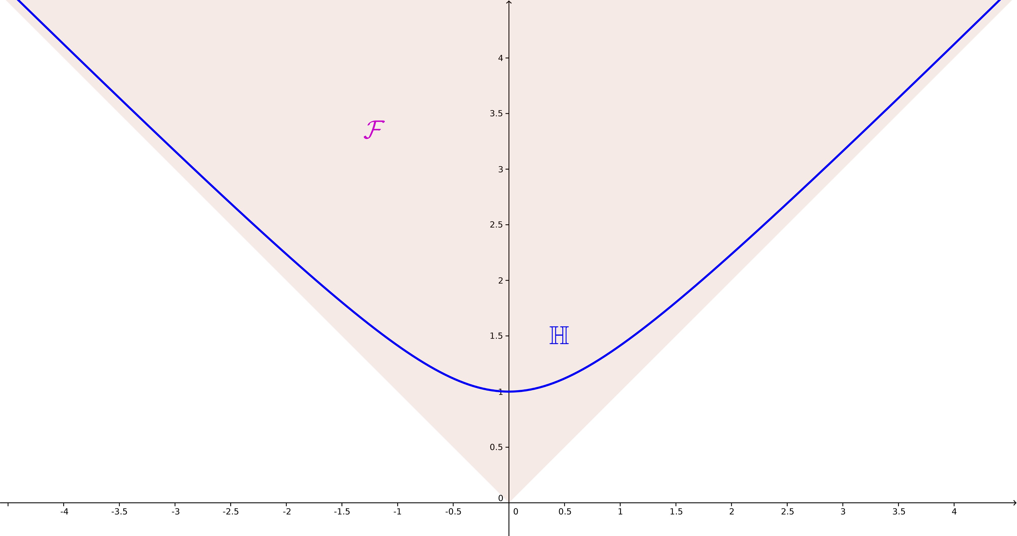
Figure 1: The cone ${\mathcal{F}}$ of future time-like vectors and the curve ${\mathbb{H}}$ of unit future time-like vectors.

${\mathcal{F}}$ and ${\mathbb{H}}$ are globally invariant under the action of the linear isometries of the Lorentzian plane, called hyperbolic translations:

$$H_{t}:=\left(\begin{array}[]{cc}\cosh t&\sinh t\\ \sinh t&\cosh t\end{array}\right),t\in{\mathbb{R}}.$$ (2)

In all the paper we fix a positive $t$. We denote by $<H_{t}>$ the free group spanned by $H_{t}$.

3 $t$-convex polygons

Let $a\in{\mathcal{F}}$. We will denote by

$$a^{\bot}:=\{x\in{\mathbb{R}}^{2}|\langle x,a\rangle_{1}=\langle a,a\rangle_{1}\}$$

the line that passes through $a$ and is parallel to the $1$-dimensional subspace orthogonal to $a$ under $\langle\cdot,\cdot\rangle_{1}$.

Definition 3.1.

Let $(\eta_{1},\ldots,\eta_{n})$, $n\geq 1$, be pairwise distinct unit future time-like vectors in the Lorentzian plane (i.e. $\eta_{i}\in{\mathbb{H}}$), and let $h_{1},\ldots,h_{n}$ be positive numbers. A $t$-convex polygon $P$ is the intersection of the half-planes bounded by the lines

$$(H_{t}^{k}(h_{i}\eta_{i}))^{\bot},\forall k\in\mathbb{Z},\forall i=1,\ldots,n.$$

The half-planes are chosen such that the vectors $\eta_{i}$ are inward pointing. The positive numbers $h_{i}$ are the support numbers of $P$.

A $t$-convex polygon is called elementary if it is defined by a single future time-like vector $\eta$ and a positive number $h$. Note that for each $k$, $(H_{t}^{k}(h\eta))^{\bot}$ is tangent to $h{\mathbb{H}}$ (the upper hyperbola with radius $h$). Hence a $t$-convex polygon is the intersection of a finite number of elementary $t$-convex polygons.

Example 3.2.

Let $t_{0}=\sinh^{-1}(1)$, so

$$H_{t_{0}}:=\left(\begin{array}[]{cc}\sqrt{2}&1\\ 1&\sqrt{2}\end{array}\right).$$

Let us denote by $P_{1}$ the elementary $t_{0}$-convex polygon defined by the vector $\eta=\binom{0}{1}$ and the number $h=1$, see Figure 2a. The elementary $t_{0}$-convex polygon $P_{2}$ of Figure 2b is obtained from $p_{1}$ by a slightly change of $\eta$ and $h$. Their intersection forms the $t_{0}$-convex polygon of Figure 2c.

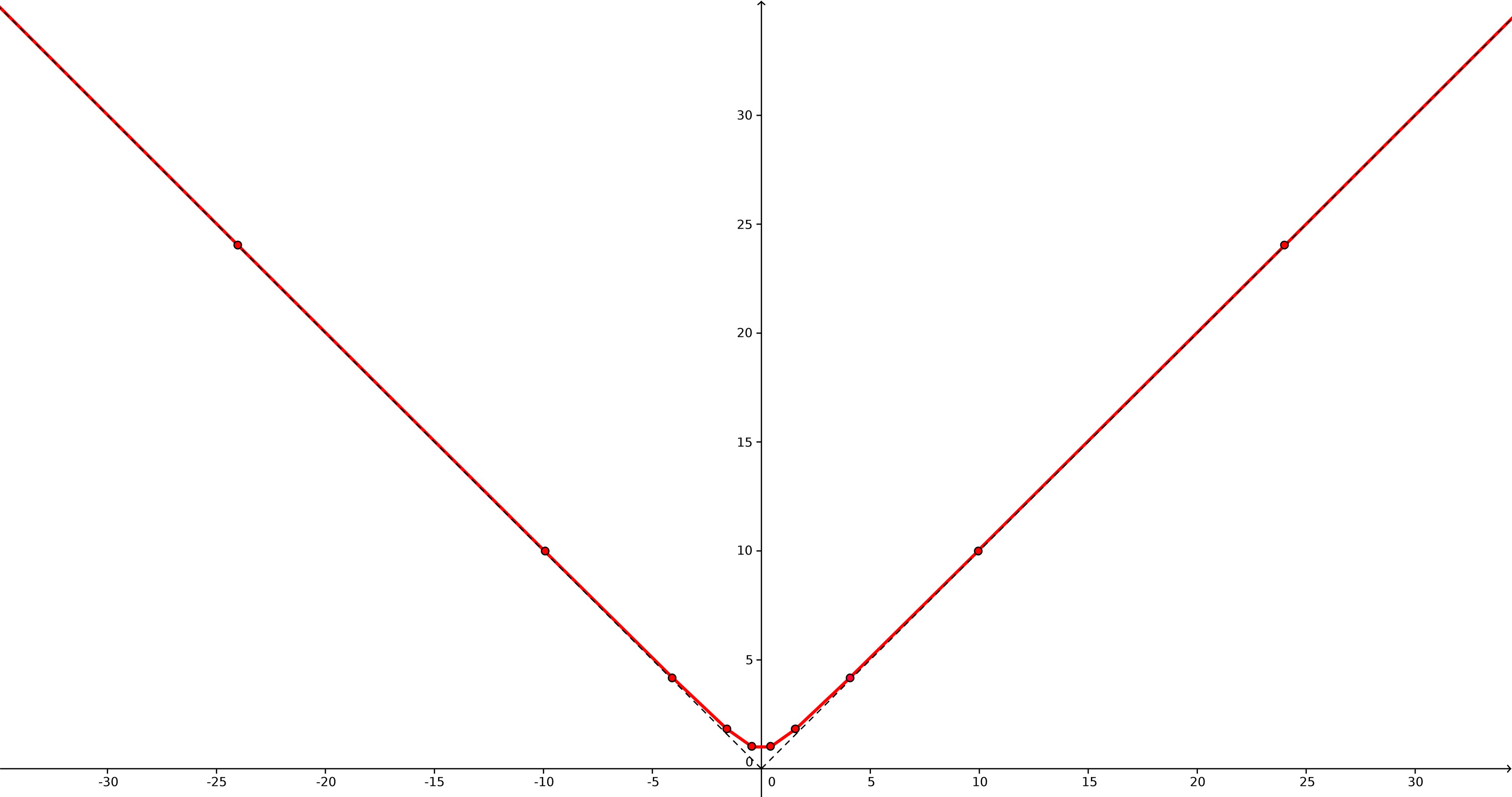
(a) A part of the $t_{0}$-convex polygon $P_{1}$. For the Lorentzian metric, all the edges have equal length and all the angles between edges are equal.

(b) A part of the $t_{0}$-convex polygon $P_{2}$. For the Lorentzian metric, all the edges have equal length and all the angles between edges are equal.

(c) A part of the $t_{0}$-convex polygon obtained as the intersection of $P_{1}$ and $P_{2}$.

Figure 2: To Example 3.2.

Lemma 3.3.

A $t$-convex polygon $P$ is a proper convex subset of ${\mathbb{R}}^{2}$ contained in ${\mathcal{F}}$, bounded by a polygonal line with a countable number of sides, and globally invariant under the action of $<H_{t}>$.

Proof.

The group invariance is clear from the definition. $P$ is the intersection of a finite number of elementary $t$-convex polygons, so we only have to check the other properties in the elementary case. Actually the only non-immediate one is that an elementary $t$-convex polygon is contained in ${\mathcal{F}}$. Let us consider an elementary $t$-convex polygon made from a single future time-like vector $\eta$ and a number $h$. Without loss of generality, consider that $h=1$. Let $u=H^{k}_{t}(\eta)$ and $v=H^{k^{\prime}}_{t}(\eta)$ and let $x$ be the intersection between $u^{\bot}$ and $v^{\bot}$. As $\langle x,u\rangle_{1}=\langle x,v\rangle_{1}=-1$, $x$ is orthogonal to $u-v$, which is a space-like vector (compute its norm with the help of (1)). Hence $x$ is time-like, and as $u^{\bot}$ and $v^{\bot}$ never meet the past cone, $x$ is future. It is easy to deduce that the $t$-convex polygon is contained in ${\mathcal{F}}$. ∎

Note that as a convex surface, a $t$-convex polygon can also be a $t^{\prime}$-convex polygon (for example it is also invariant under the action of any subgroup of $<H_{t}>$), but we will only consider the action of a given $<H_{t}>$.

Given a $t$-convex polygon $P$, we will require that the set of elementary $t$-convex polygons such that their intersection gives $P$ is minimal, i.e each $\eta_{i}$ is the inward unit normal of a genuine edge $e_{i}$ of $P$. The edge at the left (resp. right) of $e_{i}$ is denoted by $e_{i-1}$ (resp. $e_{i+1}$). Let $p_{i}$ be the foot of the perpendicular from the origin to the line containing $e_{i}$ (in particular, $p_{i}=h_{i}\eta_{i}$). Let $p_{ii+1}$ be the vertex between $e_{i}$ and $e_{i+1}$. We denote by $h_{ii+1}$ (resp. $h_{ii-1}$) the signed distance from $p_{i}$ to $p_{ii+1}$ (resp. from $p_{i}$ to $p_{i-1i}$): it is non negative if $p_{i}$ is on the same side of $e_{i+1}$ (resp. $e_{i-1}$) as $P$. The angle between $\eta_{i}$ and $\eta_{i+1}$ is denoted by $\varphi_{i}$. See Figure 3.

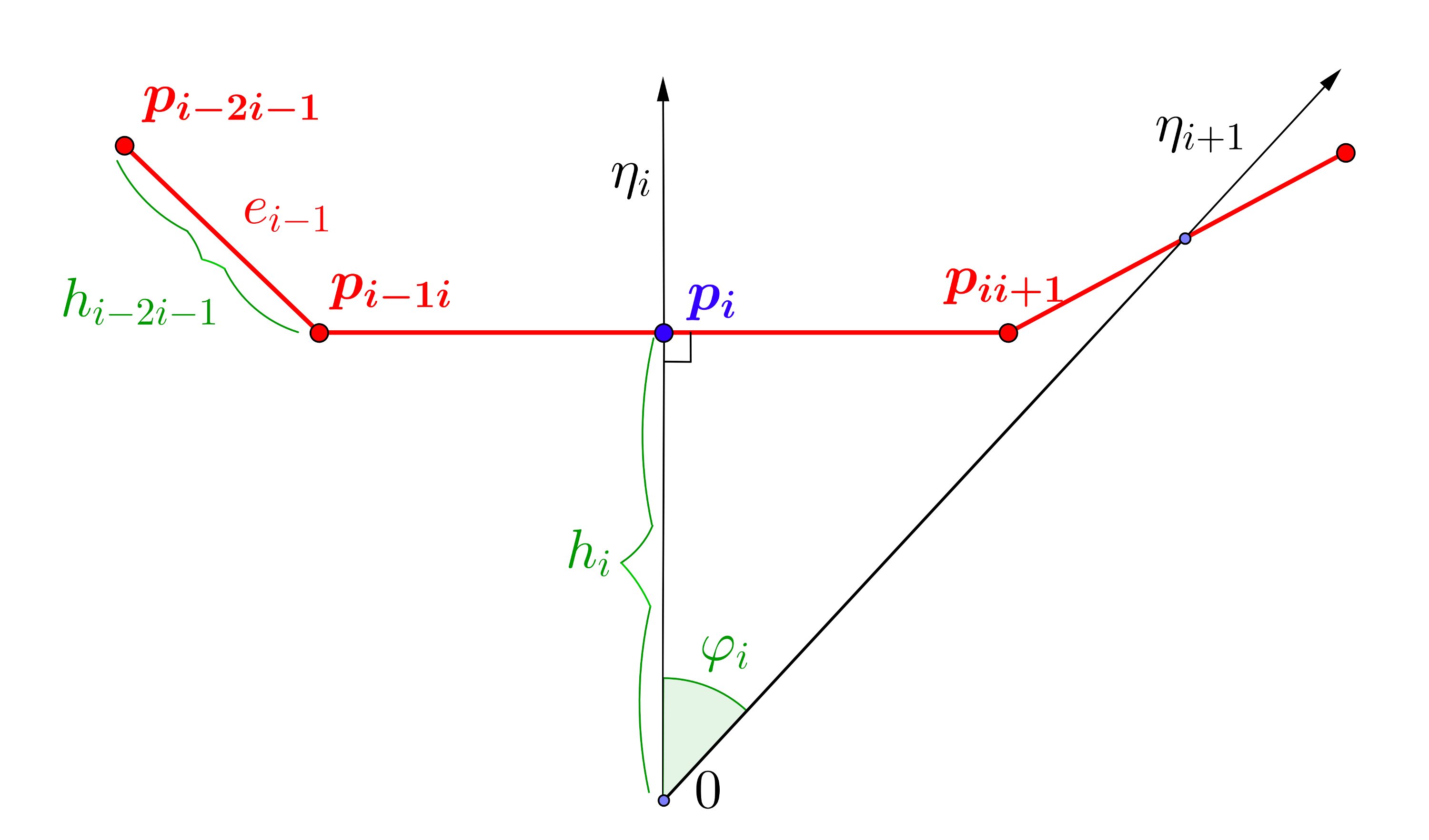
Figure 3: Notations for a $t$-convex polygon.

Lemma 3.4.

With the notations introduced above,

$$h_{ii+1}=\frac{h_{i}\cosh\varphi_{i}-h_{i+1}}{\sinh\varphi_{i}},h_{ii-1}=\frac{h_{i}\cosh\varphi_{i-1}-h_{i-1}}{\sinh\varphi_{i-1}}.$$ (3)

Proof.

By definition, $h_{ii+1}$ is non negative when $\langle p_{i}-p_{i+1},\eta_{i+1}\rangle_{1}\leq 0$, i.e.

$$-(h_{i+1}-h_{i}\cosh\varphi_{i})\geq 0.$$

Hence

$$h_{ii+1}=-\frac{h_{i+1}-h_{i}\cosh\varphi_{i}}{|h_{i+1}-h_{i}\cosh\varphi_{i}|}\sqrt{\langle p_{ii+1}-p_{i},p_{ii+1}-p_{i}\rangle_{1}}.$$

Up to an orientation and time orientation preserving linear isometry, one can take $\eta_{i}=\left(0\atop 1\right)$. In particular $p_{i}=\left(0\atop h_{i}\right)$ and $(p_{ii+1})_{2}=h_{i}$ hence

$$\langle p_{ii+1}-p_{i},p_{ii+1}-p_{i}\rangle_{1}=(p_{ii+1})_{1}^{2}.$$

We also have $\eta_{i+1}=\left(\sinh\varphi_{i}\atop\cosh\varphi_{i}\right)$, and as $\langle p_{ii+1},\eta_{i+1}\rangle_{1}=-h_{i+1}$ we get

$$(p_{ii+1})_{1}=\frac{-h_{i+1}+h_{i}\cosh\varphi_{i}}{\sinh\varphi_{i}}.$$

The proof for $h_{ii-1}$ is similar, considering $\eta_{i-1}=\left(-\sinh\varphi_{i}\atop\cosh\varphi_{i}\right)$. ∎

4 The cone of support vectors

Let $P$ be a $t$-convex polygon. Choose an edge and denote its inward unit normal by $\eta_{1}$. We denote the inward unit normal of the edge on the right by $\eta_{2}$, and so on until $\eta_{n+1}=H_{t}(\eta_{1})$. The edges with normals $\eta_{1},\ldots,\eta_{n}$ are the fundamental edges of $P$. Note that with this labeling, if $\varphi_{i}$ is the angle between $\eta_{i}$ and $\eta_{i+1}$, we have

$$\varphi_{1}+\varphi_{2}+\cdots+\varphi_{n}=t.$$ (4)

The number $h_{i}(P)$ is the support number of the edge with normal $\eta_{i}$, and $h(P)=(h_{1}(P),\ldots,h_{n}(P))$ is the support vector of $P$. So $P$ is identified with a vector of ${\mathbb{R}}^{n}$, in such a way that $\eta_{1},\ldots,\eta_{n}$ are in bijection with the standard basis of $\mathbb{R}^{n}$. Of course $P$ is uniquely determined by its support vector.

Definition 4.1.

Choose $\eta\in{\mathbb{H}}$ and let $\varphi_{1},\varphi_{2},\cdots,\varphi_{n}$ be positive numbers satisfying (4). The cone of support vectors $\overline{\mathcal{P}}(\varphi_{1},\varphi_{2},\ldots,\varphi_{n})$ is the set of support vectors of $t$-convex polygons with inward unit normals $\eta_{1}=\eta$, $\eta_{i+1}=H_{\varphi_{i}}(\eta_{i})$.

A priori the definition of $\overline{\mathcal{P}}$ depends not only on the angles $\varphi_{i}$ but also on the choice of $\eta$. Actually choosing another starting $\eta^{\prime}\in{\mathbb{H}}$, the hyperbolic translation from $\eta$ to $\eta^{\prime}$ gives a linear isomorphism between the two resulting sets of support vectors. Hence $\overline{\mathcal{P}}(\varphi_{1},\varphi_{2},\ldots,\varphi_{n})$ could be defined as the set of $t$-convex polygons with ordered angles $(\varphi_{1},\varphi_{2},\ldots,\varphi_{n})$ up to hyperbolic translations. Note also that if $s$ is a cyclic permutation, then $\overline{\mathcal{P}}(\varphi_{s(1)},\ldots,\varphi_{s(n)})$ is the same as $\overline{\mathcal{P}}(\varphi_{1},\ldots,\varphi_{n})$.

It is possible to prove that $\overline{\mathcal{P}}(\varphi_{1},\varphi_{2},\ldots,\varphi_{n})$ is a convex polyhedral cone with non-empty interior in ${\mathbb{R}}^{n}$, but this will be easier after a suitable metrization of ${\mathbb{R}}^{n}$, that is the subject of the next section.

5 Coarea

Definition 5.1.

Let $P\in\overline{\mathcal{P}}(\varphi_{1},\varphi_{2},\ldots,\varphi_{n})$. The coarea of $P$ is

$$\operatorname{coarea}(P)=\frac{1}{2}\sum_{i=1}^{n}h_{i}(P)\ell_{i}(P)$$

where the sum is on the fundamental edges, and $\ell_{i}(P)=h_{ii-1}(P)+h_{ii+1}(P)$ is the length of the $i$th fundamental edge (hence positive).

Geometrically $\operatorname{coarea}(P)$ is the area (in the sense of the Lebesgue measure) of a fundamental domain for the action of $H_{t}$ on the complement of $P$ in ${\mathcal{F}}$. The main point is that hyperbolic translations (2) have determinant $1$, so they preserve the area, which is then independent of the choice of the fundamental domain, see Figure 4. Moreover the area of a triangle with a space-like edge $e$ of length $l$ and $0$ as a vertex has area $\frac{1}{2}lh$, if $h$ is the Lorentzian distance between $0$ and the line containing $e$. (To see this, perform a hyperbolic translation such that $e$ is horizontal and compute the area.) Note that the coarea depends not only on the polygonal line $P$ but also on the group $<H_{t}>$, so it would be more precise to speak about “$t$-coarea”, but as the group is fixed from the beginning, no confusion is possible.

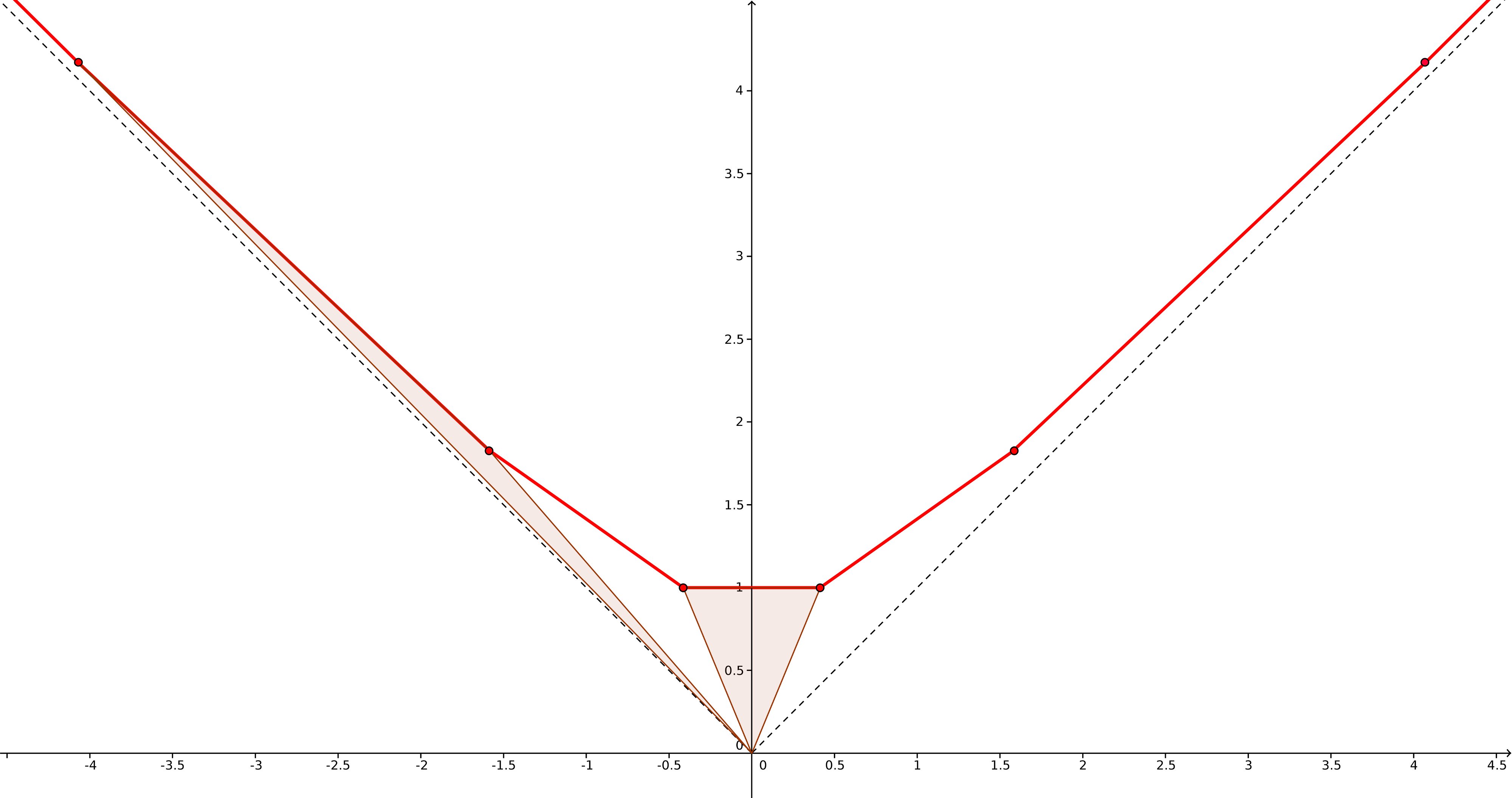
Figure 4: The two shaded regions have the same area. This area is the coarea of the polygon.

For a given cone of support vectors, the coarea can be formally extended to ${\mathbb{R}}^{n}$ with the help of (3): for $h\in{\mathbb{R}}^{n}$,

$$\operatorname{coarea}(h)=\frac{1}{2}\sum_{i=1}^{n}h_{i}\ell_{i}(h)$$

with

$$\ell_{i}(h):=\frac{h_{i}\cosh\varphi_{i-1}-h_{i-1}}{\sinh\varphi_{i-1}}+h_{i}\frac{h_{i}\cosh\varphi_{i}-h_{i+1}}{\sinh\varphi_{i}}.$$ (5)

If $n=1$, there is only one angle between the unit inward normal $\eta$ and its image under $H_{t}$, which is equal to $t$, and $\operatorname{coarea}(h)=h^{2}\frac{\cosh t-1}{\sinh t}.$

If $n\geq 2$, we introduce the mixed-coarea

$$\operatorname{coarea}(h,k)=\frac{1}{2}\sum_{i=1}^{n}h_{i}\frac{k_{i}\cosh\varphi_{i-1}-k_{i-1}}{\sinh\varphi_{i-1}}+h_{i}\frac{k_{i}\cosh\varphi_{i}-k_{i+1}}{\sinh\varphi_{i}},$$

which is the polarization of the $\operatorname{coarea}$. Actually, it is clearly a bilinear form, and

$$\operatorname{coarea}(\eta_{k},\eta_{j})=\left\{\begin{array}[]{ccc}0&\mbox{if }&2\leq|j-k|\leq n+1\\ \displaystyle{-\frac{1}{2}\frac{1}{\sinh\varphi_{k-1}}}&\mbox{if}&j=k-1\\ \displaystyle{-\frac{1}{2}\frac{1}{\sinh\varphi_{k}}}&\mbox{if}&j=k+1\\ \displaystyle{\frac{1}{2}\left(\frac{\cosh\varphi_{k-1}}{\sinh\varphi_{k-1}}+\frac{\cosh\varphi_{k}}{\sinh\varphi_{k}}\right)}&\mbox{if}&j=k\end{array}\right.$$ (6)

so $\operatorname{coarea}$ is symmetric. We also obtain the following key result.

Proposition 5.2.

The symmetric bilinear form $\operatorname{coarea}$ is positive definite.

Proof.

As $\cosh\varphi_{k}>1$, the matrix $(\operatorname{coarea}(u_{k},u_{j}))_{kj}$ is strictly diagonally dominant, and symmetric with positive diagonal entries, hence positive definite, see for example [Var00, 1.22]. ∎

The Cauchy–Schwarz inequality applied to support vectors of $t$-convex polygons gives the following reversed Minkowski inequality:

Corollary 5.3.

Let $P,Q$ be $t$-convex polygons with parallel edges. Then

$$\operatorname{coarea}(P,Q)^{2}\leq\operatorname{coarea}(P)\operatorname{coarea}(Q),$$

with equality if and only if $P$ and $Q$ are homothetic: $\exists\lambda>0,\forall i,h_{i}(P)=\lambda h_{i}(Q)$.

6 Spherical orthoschemes

$\overline{\mathcal{P}}(\varphi_{1},\varphi_{2},\ldots,\varphi_{n})$ is clearly a cone in ${\mathbb{R}}^{n}$. Moreover it is the set of vectors of positive edge lengths, for the edge lengths defined by (5). From the definition of the coaera, for $h\in{\mathbb{R}}^{n}$, $2\operatorname{coarea}(\eta_{i},h)=\ell_{i}(h)$, so $\eta_{i}$ is an inward normal vector to the facet of $\overline{\mathcal{P}}$ defined by $\ell_{i}=0$. So $\overline{\mathcal{P}}$ is polyhedral, and it is convex because the $\eta_{i}$ form a basis of ${\mathbb{R}}^{n}$. Let us denote by $\mathcal{P}(\varphi_{1},\varphi_{2},\ldots,\varphi_{n})$ the intersection of $\overline{\mathcal{P}}(\varphi_{1},\varphi_{2},\ldots,\varphi_{n})$ with the unit sphere of $({\mathbb{R}}^{n},\operatorname{coarea})$ (i.e. the set of support vectors of $t$-convex polygons with coarea one). It follows that $\mathcal{P}$ is a spherical simplex. If $n=1$, $\mathcal{P}$ is a point on a line, so from now on assume that $n>1$.

When $n=2$, $\mathcal{P}$ is an arc on the unit circle with length $\theta$ satisfying

$$\cos\theta=\frac{\sinh\varphi_{2}}{\sinh(\varphi_{1}+\varphi_{2})}.$$

When $n=3$, $\mathcal{P}$ is a spherical triangle with acute inner angles, whose cosines are given by:

$$-\frac{\operatorname{coarea}(\eta_{k},\eta_{k+1})}{\sqrt{\operatorname{coarea}(\eta_{k},\eta_{k})}\sqrt{\operatorname{coarea}(\eta_{k+1},\eta_{k+1})}}=\sqrt{\frac{\sinh\varphi_{k-1}\sinh\varphi_{k+1}}{\sinh(\varphi_{k-1}+\varphi_{k})\sinh(\varphi_{k}+\varphi_{k+1})}}.$$ (7)

When $n\geq 3$, from (6) we see that each facet has an acute interior dihedral angle with exactly two other facets, and is orthogonal to the other facets. Such spherical simplexes are called acute spherical orthoschemes. See [Deb90, 5] for the history and main properties of these very particular simplexes. Note that there are no spherical Coxeter orthoschemes, because the Coxeter diagram of a spherical orthoscheme must be a cycle, and there is no cycle in the list of Coxeter diagrams of spherical Coxeter simplexes. The list can be found for example in [Rat06].

Let us denote by $U_{k}$ the line through $p_{k}$ (so the angle between $U_{k}$ and $U_{k+1}$ is $\varphi_{k}$), and by $\lambda$ the cross ratio $[U_{k-1},U_{k},U_{k+1},U_{k+2}]$, namely if $u_{k-1},u_{k},u_{k+1},u_{k+2}$ are the intersections of the lines $U_{i}$ with any line not passing through zero and endowed with coordinates then (see [Ber94])

$$\lambda=[U_{k-1},U_{k},U_{k+1},U_{k+2}]=\frac{u_{k+1}-u_{k-1}}{u_{k+1}-u_{k}}\frac{u_{k+2}-u_{k}}{u_{k+2}-u_{k-1}}.$$

We have the formula (see [PY12])

$$\frac{\sinh\varphi_{k-1}\sinh\varphi_{k+1}}{\sinh(\varphi_{k-1}+\varphi_{k})\sinh(\varphi_{k}+\varphi_{k+1})}=\frac{\lambda-1}{\lambda}=[U_{k-1},U_{k+2},U_{k},U_{k+1}].$$

From a given $n$-dimensional acute spherical orthoscheme $O$ we can find angles (positive real numbers) $(\varphi_{1},\varphi_{2},\ldots,\varphi_{n})$ such that $\mathcal{P}(\varphi_{1},\varphi_{2},\ldots,\varphi_{n})$ is isometric to $O$. Let $0<A<1$ be the square of the cosine of an acute dihedral angle of $O$. We have first to find ordered time-like lines $U_{1},U_{2},U_{3},U_{4}$ such that $[U_{1},U_{2},U_{3},U_{4}]=\frac{1}{1-A}$, i.e. we have to prove that the cross-ratio of the lines can reach any value $>1$. Choose arbitrary distinct ordered time-like $U_{1},U_{2},U_{4}$. If $U_{3}=U_{4}$ then $[U_{1},U_{2},U_{3},U_{4}]=1$, and if $U_{3}=U_{2}$ then $[U_{1},U_{2},U_{3},U_{4}]=+\infty$, so by continuity any given value $>1$ can be reached for a suitable $U_{3}$ between $U_{2}$ and $U_{4}$. $U_{1},U_{2},U_{3},U_{4}$ give angles $\varphi_{1},\varphi_{2},\varphi_{3}$.

Now the other $\varphi_{k}$ are easily obtained as follows. Given the next dihedral angle of $O$ (they can be ordered by ordering the unit normals to $O$, see [Deb90]), the square of its cosine should be equal to

$$\frac{\sinh\varphi_{2}\sinh\varphi_{4}}{\sinh(\varphi_{2}+\varphi_{3})\sinh(\varphi_{3}+\varphi_{4})}$$

and $\varphi_{2},\varphi_{3}$ are known, so we get $\varphi_{4}$. And so on.

7 Spherical cone-manifolds

Let $n>2$ and consider the orthoscheme $\mathcal{P}=\mathcal{P}(\varphi_{1},\ldots,\varphi_{n})$. A facet of $\mathcal{P}$ is isometric to the space of $t$-convex polygons with $\eta_{1},\ldots,\hat{\eta_{i}},\ldots,\eta_{n}$ ($\hat{\eta_{i}}$ means that $\eta_{i}$ is deleted from the list) as normals to the fundamental edges. The angles between the normals are $\varphi_{1},\ldots,\varphi_{i-2},\varphi_{i-1}+\varphi_{i},\varphi_{i+1},\ldots,\varphi_{n}$. This orthoscheme is also isometric to a facet of the orthoscheme $\mathcal{P}^{\prime}$ obtained by permuting $\varphi_{i-1}$ and $\varphi_{i}$ in the list of angles. Hence we can glue $\mathcal{P}$ and $\mathcal{P}^{\prime}$ isometrically along this common facet. We denote by ${\mathcal{C}}(\varphi_{1},\ldots,\varphi_{n})$ the $(n-1)$-dimensional spherical cone-manifold obtained by gluing in this way all the $(n-1)!$ orthoschemes obtained by permutations of the list $\varphi_{1},\ldots,\varphi_{n}$, up to cyclic permutations.

When $n=3$, ${\mathcal{C}}(\varphi_{1},\varphi_{2},\varphi_{3})$ is isometric to a spherical cone-metric on the sphere with three conical singularities, with cone-angles $<\pi$, obtained by gluing two isometric spherical triangles along corresponding edges.

Let $n\geq 4$. Around the codimension 2 face of ${\mathcal{C}}$ isometric to

$$N:=\mathcal{C}(\varphi_{1},\ldots,\varphi_{k}+\varphi_{k+1},\ldots,\varphi_{j}+\varphi_{j+1},\ldots,\varphi_{n+3})$$

are glued four orthoschemes, corresponding to the four ways of ordering $(\varphi_{k},\varphi_{k+1})$ and $(\varphi_{j},\varphi_{j+1}).$ As the dihedral angle of each orthoscheme at such codimension $2$ face is $\pi/2$, the total angle around $N$ in ${\mathcal{C}}$ is $2\pi$. Hence metrically $N$ is actually not a singular set. Around the codimension 2 face of ${\mathcal{C}}$ isometric to

$$S:={\mathcal{C}}(\varphi_{1},\ldots,\varphi_{k}+\varphi_{k+1}+\varphi_{k+2},\ldots,\varphi_{n+3})$$

are glued six orthoschemes corresponding to the six ways of ordering $(\varphi_{k},\varphi_{k+1},\varphi_{k+2})$. Let $\Theta$ be the cone-angle around $S$. It is the sum of the dihedral angles of the six orthoschemes glued around it. As formula (7) is symmetric for two variables, $\Theta$ is two times the sum of three different dihedral angles. A direct computation gives ($k=1$ in the formula)

$$\cos(\Theta/2)=\textstyle\frac{\sinh\varphi_{1}\sinh\varphi_{2}\sinh\varphi_{3}-\sinh(\varphi_{1}+\varphi_{2}+\varphi_{3})(\sinh\varphi_{1}\sinh\varphi_{2}+\sinh\varphi_{2}\sinh\varphi_{3}+\sinh\varphi_{3}\sinh\varphi_{1})}{\sinh(\varphi_{1}+\varphi_{2})\sinh(\varphi_{2}+\varphi_{3})\sinh(\varphi_{3}+\varphi_{1})}.$$

During the computation we used that

$$\sinh(a+b)\sinh(b+c)-\sinh a\sinh c=\sinh b\sinh(a+b+c)$$

which can be checked with $\frac{1}{2}\left(\cosh(x+y)-\cosh(x-y)\right)=\sinh x\sinh y$. The analogous formula in the Euclidean convex polygons case was obtained in [KNY99].

For example when $\varphi_{i}=\varphi\;\forall i$, we have

$$\cos(\Theta/2)=-\frac{2\cosh(\varphi)^{2}+\sinh(\varphi)^{2}}{2\cosh(\varphi)^{3}}.$$

The function on the right-hand side is a bijection from the positive numbers to $]-1,0[$, hence all the $\Theta\in]2\pi,3\pi[$ (the dihedral angle $\theta\in]\pi/3,\pi/2[$) are uniquely reached. In particular ${\mathcal{C}}$ is not an orbifold.

The cone-manifold ${\mathcal{C}}$ comes with an isometric involution which consists of reversing the order of the angles $(\varphi_{1},\ldots,\varphi_{n})$.

8 Higher dimensional generalization

The generalization of $t$-convex polygons to higher dimensional Minkowski spaces is as follows. Let us consider the $d$-dimensional hyperbolic space ${\mathbb{H}}^{d}$ as a pseudo-sphere in the $d+1$-dimensional Minkowski space $M^{d+1}$, and let $\Gamma$ be a discrete group of linear isometry of $M^{d+1}$ such that ${\mathbb{H}}^{d}/\Gamma$ is a compact hyperbolic manifold. A $\Gamma$-convex polyhedron is, given $\eta_{1},\ldots,\eta_{n}\in{\mathbb{H}}^{d}$ and positive numbers $h_{1},\ldots,h_{n}$, the intersection of the future sides of the space-like hyperplanes $(\gamma(h_{i}\eta_{i}))^{\bot}$ $\forall i,\forall\gamma\in\Gamma$. The mixed-coarea is generalized as a “mixed covolume”. For details and computation of the signature, see [Fil13]. Actually for a given set of $\eta_{i}$, many combinatorial types may appear, and one has to restrict to type cones (cones of polyhedra with parallel facets and same combinatorics). It should be interesting to investigate the kind of spherical polytopes that appear.

Another related question is to look at the quadratic form given by the face area of the polyhedra (in a fundamental domain) and its relations with the moduli spaces of flat metric with conical singularities of negative curvature on compact surfaces of genus $>1$ (the quotient of the boundary of a $\Gamma$-convex polyhedron is isometric to such a metric).

The analogous questions in the convex polytopes case are the subject of [FI13]. The moduli space of flat metrics on the sphere was studied in [Thu98].

References

- [Ber94] M. Berger. Geometry. I. Universitext. Springer-Verlag, Berlin, 1994. Translated from the 1977 French original by M. Cole and S. Levy, Corrected reprint of the 1987 translation.
- [BG92] C. Bavard and É. Ghys. Polygones du plan et polyèdres hyperboliques. Geom. Dedicata, 43(2):207–224, 1992.
- [Deb90] H. E. Debrunner. Dissecting orthoschemes into orthoschemes. Geom. Dedicata, 33(2):123–152, 1990.
- [FI13] F. Fillastre and I. Izmestiev. Shapes of polyhedra, mixed volumes, and hyperbolic geometry. In preparation, 2013.
- [Fil11] F. Fillastre. From spaces of polygons to spaces of polyhedra following Bavard, Ghys and Thurston. Enseign. Math. (2), 57(1-2):23–56, 2011.
- [Fil13] F. Fillastre. Fuchsian convex bodies: basics of Brunn–Minkowski theory. To appear Geometric and Functional Analysis, 2013.
- [FV13] F. Fillastre and G. Veronelli. Lorentzian area measures and the Christoffel problem. 2013.
- [IH85] H.-C. Im Hof. A class of hyperbolic Coxeter groups. Exposition. Math., 3(2):179–186, 1985.
- [IH90] H.-C. Im Hof. Napier cycles and hyperbolic Coxeter groups. Bull. Soc. Math. Belg. Sér. A, 42(3):523–545, 1990. Algebra, groups and geometry.
- [KNY99] S. Kojima, H. Nishi, and Y. Yamashita. Configuration spaces of points on the circle and hyperbolic Dehn fillings. Topology, 38(3):497–516, 1999.
- [PY12] A. Papadopoulos and S. Yamada. A Remark on the Projective Geometry of Constant Curvature Spaces. 2012.
- [Rat06] J. Ratcliffe. Foundations of hyperbolic manifolds, volume 149 of Graduate Texts in Mathematics. Springer, New York, second edition, 2006.
- [Thu98] W. P. Thurston. Shapes of polyhedra and triangulations of the sphere. In The Epstein birthday schrift, volume 1 of Geom. Topol. Monogr., pages 511–549 (electronic). Geom. Topol. Publ., Coventry, 1998. Circulated as a preprint since 1987.
- [Var00] R. Varga. Matrix iterative analysis, volume 27 of Springer Series in Computational Mathematics. Springer-Verlag, Berlin, expanded edition, 2000.