High-Order Wave Propagation Algorithms for Hyperbolic Systems

Abstract

We present a finite volume method that is applicable to hyperbolic PDEs including spatially varying and semilinear nonconservative systems. The spatial discretization, like that of the well-known Clawpack software, is based on solving Riemann problems and calculating fluctuations (not fluxes). The implementation employs weighted essentially non-oscillatory reconstruction in space and strong stability preserving Runge-Kutta integration in time. The method can be extended to arbitrarily high order of accuracy and allows a well-balanced implementation for capturing solutions of balance laws near steady state. This well-balancing is achieved through the $f$-wave Riemann solver and a novel wave-slope WENO reconstruction procedure. The wide applicability and advantageous properties of the method are demonstrated through numerical examples, including problems in nonconservative form, problems with spatially varying fluxes, and problems involving near-equilibrium solutions of balance laws.

1 Introduction

Many important physical phenomena are governed by hyperbolic systems of conservation laws. In one space dimension the standard conservation law has the form

$$q_{t}+f(q)_{x}=0,$$ (1)

where the components of $q\in\mathbb{R}^{m}$ are conserved quantities and the components of $f:\mathbb{R}^{m}\times\mathbb{R}^{m}\rightarrow\mathbb{R}^{m}$ are the corresponding fluxes. Very many numerical methods have been developed for the solution of (1); some of the most successful are the high resolution Godunov-type methods based on the use of Riemann solvers and nonlinear limiters. These and other methods are generally based on flux-differencing and make explicit use of the flux function $f$.

Herein we also consider systems with spatially varying flux:

$$\kappa(x)q_{t}+f(q,x)_{x}=\psi(q,x),$$ (2)

and spatially varying linear systems not in conservation form:

$$\kappa(x)q_{t}+A(x)q_{x}=\psi(q,x),$$ (3)

as well as their two-dimensional extensions. Wave-propagation methods of up to second-order accuracy have been developed for such systems in, e.g. [22, 20]. These methods are based on wave-propagation Riemann solvers, which compute fluctuations, (i.e. traveling discontinuities) rather than fluxes and thus can be applied to (2) or (3) just as easily as to the conservation law (1).

Second-order methods may often be the best choice in terms of a balance between computational cost and desired resolution, especially for problems with solutions dominated by shocks or other discontinuities with relatively simple structures between these discontinuities. For problems containing complicated smooth solution structures, where the accurate resolution of small scales is required (e.g. simulation of compressible turbulence, computational aeroacoustics, computational electromagnetism, turbulent combustion etc.), schemes with higher order accuracy are desirable.

The purpose of this work is to present a numerical method that combines the advantages of wave-propagation solvers with high order of accuracy. The basic discretization approach was presented already in [15]; here, we give a more detailed presentation and demonstrate the wide applicability of the method. The new method combines the notions of wave propagation ([22, 24]) and the method of lines, and can in principle be extended to arbitrarily high order accuracy by the use of high order accurate spatial reconstructions and high order accurate ordinary differential equation (ODE) solvers. The implementation presented here is based on the fifth-order accurate weighted essentially non-oscillatory (WENO) reconstruction and a fourth-order accurate strong-stability-preserving Runge-Kutta (RK) scheme. We restrict our attention to problems in one or two dimensions, although the method may be extended in a straightforward manner to higher dimensions.

Although the method described here can be applied to classical hyperbolic systems (1), in that case it is equivalent to a standard finite volume WENO flux-differencing scheme, as long as component-wise reconstruction and a conservative wave propagation Riemann solver (such as a Roe or HLL solver) are used. For this reason, we focus on problems in non-conservative form or with explicit spatial dependence in the flux or source terms, which can be challenging for traditional discretizations.

Another approach to high order discretization of hyperbolic PDEs, referred to as the ADER method, has been developed by Titarev & Toro [33] and subsequent authors. That approach uses the Cauchy-Kovalewski procedure and has the advantage of leading to one-step time discretization. The method of lines approach used in the present work seems more straightforward and allows manipulation of the method’s properties by the use of different time integrators, but requires the evaluation of multiple stages per time step.

A similar class of conservative, well-balanced, and high-order accurate methods has been developed by Castro, Gallardo, Pares, and their coauthors; see, e.g. [4]. Those methods also use WENO reconstruction and Runge-Kutta time stepping in conjunction with Riemann solvers, and lead to a discretization with a form similar to that presented here and in [15]. Those methods have recently been combined with the ADER approach; see [9]. The present method differs in the approach to reconstruction and the kind of Riemann solvers used. These differences result in some useful features: our method also handles systems (2)-(3) with capacity function $\kappa$ and it can make use of $f$-wave Riemann solvers [3] as well as wave-slope reconstruction and achieve high order convergence even for some problems with discontinuous coefficients. Finally, the method can immediately be applied to very many interesting problems because the implementation is based on Clawpack Riemann solvers, which are available for a great variety of hyperbolic systems. A potential drawback of the current implementation of our method is that, for well-balancing, it relies on discretizing the source term such that its effect is collocated at cell interfaces only.

The methods described in this paper are implemented in the software package SharpClaw, which is freely available on the web at http://www.clawpack.org. SharpClaw employs the same interface that is used in Clawpack [24] for problem specification and setup, as well as for the necessary Riemann solvers. This makes it simple to apply SharpClaw to a problem that has been set up in Clawpack. These methods have also been incorporated into PyClaw[17], which allows them to be run in parallel on large supercomputers.

The paper is organized as follows. In Section 2.2, we present Godunov’s method for linear hyperbolic PDEs in wave propagation form [24]. This method is extended to high order in Section 2.3 by introducing a high-order reconstruction based on cell averages. Generalization to spatially varying nonconservative linear systems is presented in 2.4. Further extensions and details of the method are presented in the remainder of Section 2. Numerical examples, including application to acoustics, elasticity, and shallow water waves,are presented in Section 3.

2 Semi-discrete wave-propagation

The wave-propagation algorithm was first introduced by LeVeque [22] in 1997 in the framework of high resolution finite volume methods for solving hyperbolic systems of equations. The scheme is conservative, second-order accurate in smooth regions, and captures shocks without introducing spurious oscillations. In this section, we extend the wave-propagation algorithm to high order accuracy through use of high order reconstruction and time marching. For simplicity, we focus on the one dimensional scheme and then briefly describe the extension to two dimensions.

2.1 Riemann Problems and Notation

The notation for Riemann solutions used in this paper comes primarily from [24], and is motivated by consideration of the linear hyperbolic system

$$q_{t}+Aq_{x}=0.$$ (4)

Here $q\in\mathbb{R}^{m}$ and $A\in\mathbb{R}^{m\times m}$. System (4) is said to be hyperbolic if $A$ is diagonalizable with real eigenvalues; we will henceforth assume this to be the case. Let $s^{p}$ and $r^{p}$ for $1\leq p\leq m$ denote the eigenvalues and the corresponding right eigenvectors of $A$ with the eigenvalues ordered so that $s^{1}\leq s^{2}\leq\ldots\leq s^{m}$.

Consider the Riemann problem consisting of (4) together with initial data

$$q(x,0)=\left\{\begin{array}[]{cc}q_{l}&x<0\\ q_{r}&x>0\end{array}\right..$$ (7)

The solution for $t>0$ is piecewise constant with $m$ discontinuities, the $p$th one proportional to $r^{p}$ and moving at speed $s^{p}$. They can be obtained by decomposing the difference $q_{r}-q_{l}$ in terms of the eigenvectors $r^{p}$:

$$q_{r}-q_{l}=\sum_{p}\alpha^{p}r^{p}=\sum_{p}{\cal W}^{p}.$$ (8)

We refer to the vectors ${\cal W}^{p}$ as waves. Each wave is a jump discontinuity along the ray $x=s^{p}t$. An example solution is pictured in Figure 1 for $m=3$. For brevity, we will sometimes refer to the Riemann problem with initial left state $q_{l}$ and initial right state $q_{r}$ as the Riemann problem with initial states $(q_{l},q_{r})$.

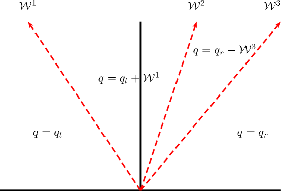
Fig. 1: The wave propagation solution of the Riemann problem. The horizontal axis corresponds to space and the vertical axis to time.

In a finite volume method, it is useful to define notation for the net effect of all left- or right-going waves:

$${\cal A}^{-}\Delta q \equiv \sum_{p=1}^{m}\left(s^{p}\right)^{-}{\cal W}^{p}$$ (9a)

$${\cal A}^{+}\Delta q \equiv \sum_{p=1}^{m}\left(s^{p}\right)^{+}{\cal W}^{p}.$$ (9b)

Here and throughout, $(x)^{\pm}$ denotes the positive or negative part of $x$:

$$(x)^{-}=\min(x,0)\quad\quad(x)^{+}=\max(x,0).$$

The symbols ${\cal A}^{\pm}\Delta q$, referred to as fluctuations, should be interpreted as single entities that represent the net effect of all waves travelling to the right or left. The notation is motivated by the constant coefficient linear system (4), in which case ${\cal A}^{\pm}\Delta q=A^{\pm}(q_{r}-q_{l})$, where $A^{-}$ (respectively $A^{+}$) is the matrix obtained by setting all postive (respectively negative) eigenvalues of $A$ to zero. See [22] or [24] for more details.

The notation for waves and fluctuations defined in (8) and (9) can also be used to describe numerical solutions of Riemann problems for nonlinear systems if the numerical solver approximates the solution by a series of propagating jump discontinuities, which is very often the case. Because the approximate Riemann solution for a nonlinear system depends not only on the difference $q_{r}-q_{l}$ but on the values of the states, we will sometimes employ for clarity the notation ${\cal W}^{p}(q_{l},q_{r})$ to denote the $p$th wave in the solution of the Riemann problem with initial states $(q_{l},q_{r})$. In this case the vectors $r^{p}$ used for the decomposition (8) are typically eigenvectors of an averaged Jacobian matrix $\bar{A}$, and the $s^{p}$ are the corresponding wave speeds. Then ${\cal A}^{\pm}\Delta q=\bar{A}^{\pm}(q_{r}-q_{l})$. But there are other possible ways to define the $r^{p}$, $s^{p}$ and hence the fluctuations. For example, using the HLL approximate Riemann solver [12] would always use only two waves regardless of the size of the system. Or, for the case of spatially varying flux functions, the left-going waves may be defined by eigenvectors of the Jacobian $f^{\prime}(q_{l})$ while the right-going waves are defined by eigenvectors of the Jacobian $f^{\prime}(q_{r})$. One could combine these to create a matrix $\bar{A}$ having this set of eigenvectors and the corresponding eigenvalues, but this is not required for implementation of the method. For these reasons we use the more general notation ${\cal A}^{\pm}\Delta q$ for the fluctuations defined by (9).

2.2 First-order Godunov’s method

Consider the constant-coefficient linear system in one dimension (4). Taking a finite volume approach, we define the cell averages (i.e. the solution variables)

$$Q_{i}(t)=\frac{1}{\Delta x}\int_{x_{i-\frac{1}{2}}}^{x_{i+\frac{1}{2}}}q(x,t)dx,$$

where the index $i$ and the quantity $\Delta x$ denote the cell index and the cell size, respectively. To solve the linear system (4), we initially approximate the solution $q(x,t)$ by these cell averages; that is, at $t=t_{0}$ we define the piecewise-constant function

$$\tilde{q}(x,t_{0})=Q_{i}\mbox{ for }x\in(x_{i-\frac{1}{2}},x_{i+\frac{1}{2}}).$$ (10)

The linear system (4) with initial data $\tilde{q}$ consists locally of a series of Riemann problems, one at each interface $x_{i-\frac{1}{2}}$. The Riemann problem at $x_{i-\frac{1}{2}}$ consists of (4) with the piecewise constant initial data

$$q(x,0)=\left\{\begin{array}[]{ll}Q_{i-1}&x<x_{i-\frac{1}{2}}\\ Q_{i}&x>x_{i-\frac{1}{2}}\end{array}\right..$$

As discussed above, the solution of the Riemann problem is expressed as a set of waves obtained by decomposing the jump in $Q$ in terms of the eigenvectors of $A$:

$$Q_{i}-Q_{i-1}=\sum_{p}\alpha^{p}_{i-\frac{1}{2}}r^{p}_{i-\frac{1}{2}}=\sum_{p}{\cal W}^{p}(Q_{i-1},Q_{i}).$$ (11)

Let $\tilde{q}(x,t_{0}+\Delta t)$ denote the exact evolution of $\tilde{q}$ after a time increment $\Delta t$. If we take $\Delta t$ small enough that the waves from adjacent interfaces do not pass through more than one cell, then we can integrate (4) over $[x_{i-\frac{1}{2}},x_{{i+\frac{1}{2}}}]\times[0,\Delta t]$ and divide by $\Delta x$ to obtain

$$Q_{i}(t_{0}+\Delta t)-Q_{i}(t_{0}) =-\frac{1}{\Delta x}\int_{x_{i-\frac{1}{2}}}^{x_{i+\frac{1}{2}}}A\,\tilde{q}_{x}(x,t_{0}+\Delta t)dx.$$ (12)

Here $\tilde{q}_{x}$ should be understood in the sense of distributions.

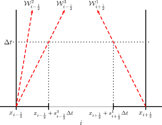
Fig. 2: Time evolution of the reconstructed solution $\tilde{q}$ in cell $i$.

We can split the integral above into three parts, representing the Riemann fans from the two interfaces, and the remaining piece:

$$\int_{x_{i-\frac{1}{2}}}^{x_{i+\frac{1}{2}}}A\tilde{q}_{x}dx =\int_{x_{i-\frac{1}{2}}}^{x_{i-\frac{1}{2}}+s^{R}\Delta t}A\tilde{q}_{x}dx+\int_{x_{i+\frac{1}{2}}+s^{L}\Delta t}^{x_{i+\frac{1}{2}}}A\tilde{q}_{x}dx+\int_{x_{i-\frac{1}{2}}+s^{R}\Delta t}^{x_{i+\frac{1}{2}}+s^{L}\Delta t}A\tilde{q}_{x}dx.$$ (13)

The relevant regions are depicted in Figure 2. Here we have defined $s^{L}=\min(s^{1}_{i+\frac{1}{2}},0)$ and $s^{R}=\max(s^{m}_{i-\frac{1}{2}},0)$. The third integral in (13) vanishes because $\tilde{q}(x,\Delta t)$ is constant outside the Riemann fans, by the definition (10). Hence (13) reduces to

$$\int_{x_{i-\frac{1}{2}}}^{x_{i+\frac{1}{2}}}A\tilde{q}_{x}dx =\Delta t\sum_{p=1}^{m}\left(s^{p}_{i-\frac{1}{2}}\right)^{+}{\cal W}^{p}_{i-\frac{1}{2}}+\Delta t\sum_{p=1}^{m}\left(s^{p}_{i+\frac{1}{2}}\right)^{-}{\cal W}^{p}_{i+\frac{1}{2}}$$ (14a)

$$=\Delta t\left({\cal A}^{+}\Delta Q_{i-\frac{1}{2}}+{\cal A}^{-}\Delta Q_{i+\frac{1}{2}}\right),$$ (14b)

where the fluctuations ${\cal A}^{-}\Delta Q_{i+\frac{1}{2}}$ and ${\cal A}^{+}\Delta Q_{i-\frac{1}{2}}$ are defined by

$${\cal A}^{-}\Delta Q_{i+\frac{1}{2}} \equiv \sum_{p=1}^{m}\left(s^{p}_{i+\frac{1}{2}}\right)^{-}{\cal W}^{p}_{i+\frac{1}{2}},\qquad{\cal W}^{p}_{i+\frac{1}{2}}\equiv{\cal W}^{p}(Q_{i},Q_{i+1})$$ (15a)

$${\cal A}^{+}\Delta Q_{i-\frac{1}{2}} \equiv \sum_{p=1}^{m}\left(s^{p}_{i-\frac{1}{2}}\right)^{+}{\cal W}^{p}_{i-\frac{1}{2}},\qquad{\cal W}^{p}_{i-\frac{1}{2}}\equiv{\cal W}^{p}(Q_{i-1},Q_{i}).$$ (15b)

Note again that the fluctuations ${\cal A}^{+}\Delta Q_{i-\frac{1}{2}}$ and ${\cal A}^{-}\Delta Q_{i+\frac{1}{2}}$ are motivated by the idea of a matrix-vector product but should be interpreted as single entities that represent the net effect of all waves travelling to the right or left. The upper-case $Q$ in the fluctuations is meant to emphasize that they are based on differences of cell averages. For instance, the fluctuation ${\cal A}^{+}\Delta Q_{i-\frac{1}{2}}$ corresponds to the effect of right-going waves from the Riemann problem with initial states $(Q_{i-1},Q_{i})$.

Substituting (14b) into (12), we obtain the scheme

$$Q_{i}^{n+1}-Q_{i}^{n}=-\frac{\Delta t}{\Delta x}\left({\cal A}^{+}\Delta Q_{i-\frac{1}{2}}+{\cal A}^{-}\Delta Q_{i+\frac{1}{2}}\right).$$

Dividing by $\Delta t$ and taking the limit as $\Delta t$ approaches zero, we obtain the semi-discrete wave-propagation form of the (first-order) Godunov’s scheme

$$\frac{\partial Q_{i}}{\partial t}=-\frac{1}{\Delta x}\left({\cal A}^{+}\Delta Q_{i-\frac{1}{2}}+{\cal A}^{-}\Delta Q_{i+\frac{1}{2}}\right).$$ (16)

Equation (16) constitutes a linear system of ordinary differential equations (ODEs) that may be integrated, for instance, with a Runge-Kutta method. It is clear from the derivation that this scheme reduces to the corresponding flux-differencing scheme when applied to systems written in conservation form, e.g. system (2).

2.3 Extension to higher order

The method of the previous section is only first-order accurate in space. In order to improve the spatial accuracy, we replace the piecewise-constant approximation (10) by a piecewise-polynomial approximation that is accurate to order $p$ in regions where the solution is smooth:

$$\tilde{q}(x,t_{0}) =\tilde{q}_{i}(x)\mbox{ for }x\in(x_{i-\frac{1}{2}},x_{i+\frac{1}{2}}),$$ (17)

where

$$\tilde{q}_{i}(x)=q(x,t_{0})+{\cal O}(\Delta x^{p+1}).$$

Integration of $A\tilde{q}_{x}$ over $[x_{i-\frac{1}{2}},x_{{i+\frac{1}{2}}}]$ again yields (13), but now the third integral is non-zero in general, since $\tilde{q}$ is not constant outside the Riemann fans. Define

$$q^{R}_{i-\frac{1}{2}}\equiv\lim_{x\to x_{i-\frac{1}{2}}^{+}}\tilde{q}_{i}(x)\qquad\qquad q^{L}_{i+\frac{1}{2}}\equiv\lim_{x\to x_{i+\frac{1}{2}}^{-}}\tilde{q}_{i}(x),$$ (18)

where superscripts $L$ and $R$ refer respectively to the left and the right state of the interface considered. Then in place of (14), we now obtain (neglecting terms of order ${\cal O}(\Delta t^{2})$)

$$\int_{x_{i-\frac{1}{2}}}^{x_{i+\frac{1}{2}}}A\tilde{q}_{x}dx \approx\Delta t\sum_{p=1}^{m}\left(s^{p}_{i-\frac{1}{2}}\right)^{+}{\cal W}^{p}_{i-\frac{1}{2}}+\Delta t\sum_{p=1}^{m}\left(s^{p}_{i+\frac{1}{2}}\right)^{-}{\cal W}^{p}_{i+\frac{1}{2}}+\int_{x_{i-\frac{1}{2}}+s^{R}\Delta t}^{x_{i+\frac{1}{2}}+s^{L}\Delta t}A\tilde{q}_{x}dx$$ (19a)

$$=\Delta t\left({\cal A}^{+}\Delta{q}_{i-\frac{1}{2}}+{\cal A}^{-}\Delta{q}_{i+\frac{1}{2}}\right)+A(q^{L}_{i+\frac{1}{2}}-q^{R}_{i-\frac{1}{2}}).$$ (19b)

The resulting fully-discrete scheme is thus

$$Q_{i}^{n+1}-Q_{i}^{n}=-\frac{\Delta t}{\Delta x}\left({\cal A}^{+}\Delta{q}_{i-\frac{1}{2}}+{\cal A}^{-}\Delta{q}_{i+\frac{1}{2}}+A(q^{L}_{i+\frac{1}{2}}-q^{R}_{i-\frac{1}{2}})\right).$$

We use the notation ${\cal A}^{\pm}\Delta{q}$ instead of ${\cal A}^{\pm}\Delta Q$ because the states in the Riemann problems are not the cell averages, but rather the reconstructed interface values. In other words, the fluctuations at $x_{i-\frac{1}{2}}$ are defined by

$${\cal A}^{\pm}\Delta{q}_{i-\frac{1}{2}} =\sum_{p=1}^{m}\left(s^{p}(q^{L}_{i-\frac{1}{2}},q^{R}_{i-\frac{1}{2}})\right)^{\pm}{\cal W}^{p}(q^{L}_{i-\frac{1}{2}},q^{R}_{i-\frac{1}{2}}).$$

For instance, the fluctuation ${\cal A}^{+}\Delta{q}_{i-\frac{1}{2}}$ corresponds to the effect of right-going waves from the Riemann problem with initial states $(q^{L}_{i-\frac{1}{2}},q^{R}_{i-\frac{1}{2}})$. Moreover, we can view the term $A(q^{L}_{i+\frac{1}{2}}-q^{R}_{i-\frac{1}{2}})$ as the sum of both the left- and right-going fluctuations resulting from a Riemann problem with initial states $(q^{R}_{i-\frac{1}{2}},q^{L}_{i+\frac{1}{2}})$. It is natural to denote this term, which we refer to as a total fluctuation, by ${\cal A}\Delta q_{i}$:

$${\cal A}\Delta q_{i} =\sum_{p=1}^{m}\left(s^{p}(q^{R}_{i-\frac{1}{2}},q^{L}_{i+\frac{1}{2}})\right)^{\pm}{\cal W}^{p}(q^{R}_{i-\frac{1}{2}},q^{L}_{i+\frac{1}{2}}).$$

Dividing by $\Delta t$ and taking the limit as $\Delta t$ approaches zero, we obtain the semi-discrete scheme

$$\frac{\partial Q_{i}}{\partial t}=-\frac{1}{\Delta x}\left({\cal A}^{+}\Delta{q}_{i-\frac{1}{2}}+{\cal A}^{-}\Delta{q}_{i+\frac{1}{2}}+{\cal A}\Delta q_{i}\right).$$ (20)

2.4 Spatially varying linear systems

Next we generalize the method to solve one-dimensional spatially varying nonconservative linear systems:

$$q_{t}+A(x)q_{x}=0.$$ (21)

We again assume that $A$ is a constant function of $x$ within each cell, so we can write $A(x)=A_{i}(q)$. In the special case that $A$ is the Jacobian matrix of some function $f$, (21) corresponds to the conservation law (1). Our method can be applied to the general system (21) as long as the physically meaningful solution to the Riemann problem can be approximated. This may be nontrivial for a nonconservative nonlinear problem, as discussed in many papers such as [5, 6, 7, 8, 19]. We do not go into this here, but assume that our numerical approach is to be applied to a problem for which the user has a means of solving the Riemann problem in terms of discontinuities (waves) ${\cal W}^{p}_{i-\frac{1}{2}}$ propagating at speeds $s^{p}_{i-\frac{1}{2}}$, and hence can define fluctuations. This is the case for any linearized Riemann solver, and often for other approximate solvers. Then the scheme is given by

$$\frac{\partial Q_{i}}{\partial t}=-\frac{1}{\Delta x}\left({\cal A}^{+}\Delta{q}_{i-\frac{1}{2}}+{\cal A}^{-}\Delta{q}_{i+\frac{1}{2}}+\int_{x_{i-\frac{1}{2}}}^{x_{i+\frac{1}{2}}}A_{i}\,\tilde{q}_{x}dx\right).$$ (22)

In general, the integral in (22) must be evaluated by quadrature; however, for the conservative system (1), the integral can be evaluated exactly, and is given by

$$\int_{x_{i-\frac{1}{2}}}^{x_{i+\frac{1}{2}}}A_{i}\,\tilde{q}_{x}dx=f(q^{L}_{i+\frac{1}{2}})-f(q^{R}_{i-\frac{1}{2}}).$$ (23)

If the fluctuations are computed using a Roe solver or some other conservative wave-propagation Riemann solver, then the flux difference appearing in (23) is equal to the sum of fluctuations from a fictitious “internal” Riemann problem for the current cell $i$, just as in the linear case above:

$$f(q^{L}_{i+\frac{1}{2}})-f(q^{R}_{i-\frac{1}{2}})={\cal A}^{+}\Delta{q}_{i}+{\cal A}^{-}\Delta{q}_{i}={\cal A}\Delta q_{i}.$$ (24)

Specifically, the fluctuations ${\cal A}^{\pm}\Delta{q}_{i}$ are those resulting from the Riemann problem with initial states $(q^{R}_{i-\frac{1}{2}},q^{L}_{i+\frac{1}{2}})$. Then we can write (22) also as

$$\frac{\partial Q_{i}}{\partial t}=-\frac{1}{\Delta x}\left({\cal A}^{-}\Delta{q}_{i+\frac{1}{2}}+{\cal A}^{+}\Delta{q}_{i-\frac{1}{2}}+{\cal A}\Delta q_{i}\right).$$ (25)

Note that, for the conservative system (1), if a Roe solver or an $f$-wave solver (see Section 2.6) is used, then the fluctuations are equal to the flux differences

$${\cal A}^{-}\Delta{q}_{i-\frac{1}{2}} = \hat{f}_{i-\frac{1}{2}}-f(q^{L}_{i-\frac{1}{2}})$$ (26)

$${\cal A}^{+}\Delta{q}_{i-\frac{1}{2}} = f(q^{R}_{i-\frac{1}{2}})-\hat{f}_{i-\frac{1}{2}},$$ (27)

where $\hat{f}_{i-\frac{1}{2}}$ is the numerical flux at $x_{i-\frac{1}{2}}$. Thus (25) is in that case equivalent to the traditional flux-differencing method

$$\frac{\partial Q_{i}}{\partial t}=-\frac{1}{\Delta x}\left(\hat{f}_{i+\frac{1}{2}}-\hat{f}_{i-\frac{1}{2}}\right).$$ (28)

In particular, the scheme is conservative in this case.

2.5 Capacity-form differencing

In many applications the system of conservation laws takes the form

$$\kappa(x)q_{t}+f(q)_{x}=0,$$ (29)

in one space dimension, or

$$\kappa(x,y)q_{t}+f(q)_{x}+g(q)_{y}=0,$$ (30)

in two dimensions, where $\kappa$ is a given function of space and is usually indicated as capacity function (see [22]). Systems like (29) and (30) arise naturally in the derivation of a conservation law, where the flux of a quantity is naturally defined in terms of one variable $q$, whereas it is a different quantity $\kappa q$ that is conserved. For instance, for the flow in a porous media, $\kappa$ would be the porosity. Note that a capacity function can also appear in systems that are not in conservation form, e.g. the quasilinear system (3).

Several approaches can be used to reduce such a system to a more familiar conservation law. One natural approach is the capacity-form differencing [22],

$$\frac{\partial Q_{i}}{\partial t}=-\frac{1}{\kappa_{i}\Delta x}\left({\cal A}^{+}\Delta{q}_{i-\frac{1}{2}}+{\cal A}^{-}\Delta{q}_{i+\frac{1}{2}}+{\cal A}\Delta q_{i}\right),$$ (31)

where $\kappa_{i}$ is the capacity of the $i$th cell. This is a simple extension of (20) or (25) which ensures that $\sum\kappa_{i}Q_{i}$ is conserved (except possibly at the boundaries) and yet allows the Riemann solution to be computed based on $q$ as in the case $\kappa=1$.

2.6 $f$-wave Riemann solvers and well-balancing

For application to conservation laws, it is desirable to ensure that the wave-propagation discretization is conservative. This can easily be accomplished by using an $f$-wave Riemann solver [3]. Use of $f$-wave solvers is also useful for problems with spatially varying flux function, as well as problems involving balance laws near steady state. Further uses of the $f$-wave approach can be found in [1, 2, 18, 28, 32].

The idea of the $f$-wave splitting for (1) is to decompose the flux difference $f(q_{r})-f(q_{l})$ into waves rather than the $q$-difference used in (11), i.e. we decompose the flux difference as a linear combination of the right eigenvectors $r^{p}$ of some Jacobian:

$$f(q_{r})-f(q_{l})=\sum_{p}\beta^{p}r^{p}=\sum_{p}\mathcal{Z}^{p}(q_{l},q_{r}).$$ (32)

The fluctuations are then defined as

$${\cal A}^{-}\Delta q \equiv\sum_{p:s^{p}<0}\mathcal{Z}^{p}(q_{l},q_{r}) {\cal A}^{+}\Delta q \equiv\sum_{p:s^{p}>0}\mathcal{Z}^{p}(q_{l},q_{r})$$

Note that the total fluctuation in cell $i$ is given simply by

$${\cal A}\Delta q_{i}=f\left(q^{L}_{i+\frac{1}{2}}\right)-f\left(q^{R}_{i-\frac{1}{2}}\right).$$

An advantage of particular interest is the possibility to include source terms directly into the $f$-wave decomposition. In fact, for balance laws that include non-hyperbolic terms,

$$q_{t}+f(q)_{x}=\psi(q,x),$$

one can easily extend this algorithm by first discretizing the source term to obtain values $\Psi_{i-\frac{1}{2}}$ at the cell interfaces and then compute the waves $\mathcal{Z}^{p}_{i-\frac{1}{2}}$ by splitting

$$f(q_{r})-f(q_{l})-\Delta x\Psi(q_{l},q_{r},x)=\sum_{p}\beta^{p}r^{p}=\sum_{p}\mathcal{Z}^{p}(q_{l},q_{r}).$$ (33)

Here $\Psi(q_{l},q_{r},x)$ is some suitable average of $\psi(q,x),$ between the neighboring states. In Bale et al. [3], it has been shown that for the second-order FV wave-propagation scheme implemented in Clawpack, the $f$-wave approach is very useful for handling source terms, especially in cases where the solution is close to a steady state because it leads to a well-balanced scheme. However, for our high order wave-propagation scheme, application of the $f$-wave algorithm with component-wise or characteristic-wise reconstruction [29] (which take no account of the source term) does not lead to a method that is well-balanced, even though the source term is accounted for in the Riemann solves which compute ${\cal A}^{\pm}\Delta{q}_{i-\frac{1}{2}}$. This is because with the aforementined WENO approaches the reconstructed solution within each cell is not constant (i.e. $q^{L}_{i+\frac{1}{2}}\neq q^{R}_{i-\frac{1}{2}}$) and ${\cal A}\Delta q_{i}\neq 0$.

In this work, we consider an extension of the $f$-wave well-balancing technique that is compatible with our higher order scheme. The extension is useful for problems in which the source term vanishes over the interior of each cell (i.e., its effect is concentrated at cell interfaces). This is the case, for instance, when considering the shallow water equations with piecewise-constant bathymetry (see Section 3.3.2). This well-balancing technique uses the $f$-wave Riemann solver in combination with a $f$-wave-slope reconstruction (see Section 2.7.3). With this approach, the contribution of the source term is directly included in the Riemann solve at the cell’s interface, i.e. (33). The reconstruction methods considered in this work are presented in the next section.

2.7 Reconstruction

The reconstruction (17) should be performed in a manner that yields high order accuracy but avoids spurious oscillations near discontinuities. For this purpose, we use weighted essentially non-oscillatory (WENO) reconstruction [31]. The spatial accuracy of the method will in general be equal to that of the reconstruction. In the present work we employ fifth-order WENO reconstruction.

2.7.1 Scalar WENO Reconstruction

WENO reconstruction formulas are typically written in terms of the divided differences $\Delta Q_{{i\pm\frac{1}{2}}}/\Delta x$. It is possible to rewrite them in terms of the difference ratios

$$\theta_{{i-\frac{1}{2}},j}=\frac{\Delta Q_{{i-\frac{1}{2}}+j}}{\Delta Q_{i-\frac{1}{2}}}.$$ (34)

as long as $\Delta Q_{i-\frac{1}{2}}\neq 0$. Then the reconstructed interface values in cell $i$ are given by

$$q^{R}_{i-\frac{1}{2}} =Q_{i}-\phi(\theta_{{i-\frac{1}{2}},2-k},\dots,\theta_{{i-\frac{1}{2}},k-1})\Delta Q_{i-\frac{1}{2}}$$ (35a)

$$q^{L}_{i+\frac{1}{2}} =Q_{i}+\phi(\theta_{{i+\frac{1}{2}},1-k},\dots,\theta_{{i+\frac{1}{2}},k-2})\Delta Q_{i-\frac{1}{2}},$$ (35b)

where $\phi$ is a particular nonlinear function that we will not write out here. The usefulness of (35) is that it allows WENO reconstruction to be applied to waves directly by redefining $\theta$, as we do below. In the case that $\Delta Q_{i-\frac{1}{2}}\approx 0$ (to near machine precision), the value of $\phi$ is set to zero.

For systems of equations, the simplest approach to reconstruction is component-wise reconstruction, which consists of applying the scalar reconstruction approach (34)-(35) to each element of $q$. A more sophisticated approach is characteristic-wise reconstruction, in which an eigendecomposition of $q$ is performed, followed by reconstruction of each eigencomponent. For problems with spatially-varying coefficients, even the characteristic-wise reconstruction may not be satisfying, since it involves comparing coefficients of eigenvectors whose direction in state space varies from one cell to the next. In Clawpack, an alternative kind of TVD limiting known as wave limiting has been implemented and shown to be effective for such problems.

2.7.2 Wave-slope reconstruction

In order to implement a wave-type WENO limiter, we first solve a Riemann problem at each interface $x_{i-\frac{1}{2}}$, using the adjacent cell average values $Q_{i-1},Q_{i}$ as left and right states. This results in a set of waves ${\cal W}^{p}_{i-\frac{1}{2}}$, which are used solely for the purpose of reconstruction. This reconstruction is performed by replacing (34) by

$$\theta^{p}_{{i-\frac{1}{2}},j} =\frac{{\cal W}^{p}_{i-\frac{1}{2}+j}\cdot{\cal W}^{p}_{i-\frac{1}{2}}}{{\cal W}^{p}_{i-\frac{1}{2}}\cdot{\cal W}^{p}_{i-\frac{1}{2}}}$$ (36)

and replacing (35) by

$$q^{L}_{i-\frac{1}{2}} =Q_{i-1}+\sum_{p}\phi(\theta^{p}_{{i+\frac{1}{2}},1-k},\dots,\theta^{p}_{{i+\frac{1}{2}},k-2}){\cal W}^{p}_{i-\frac{1}{2}}$$ (37a)

$$q^{R}_{i-\frac{1}{2}} =Q_{i}\ \ \ -\sum_{p}\phi(\theta^{p}_{{i-\frac{1}{2}},2-k},\dots,\theta^{p}_{{i-\frac{1}{2}},k-1}){\cal W}^{p}_{i-\frac{1}{2}},$$ (37b)

This approach takes into account the smoothness of the $p$th characteristic component of the solution by using the information arising from the $k$-cell stencils. It is intended to be similar to that used in Clawpack [24] and can be conveniently implemented using the same Riemann solvers supplied with Clawpack.

2.7.3 $f$-wave-slope reconstruction

Wave-slope reconstruction can also be performed using an $f$-wave Riemann solver. This is useful for computing near-equilibrium solutions of balance laws. The procedure is identical to that above, except that the Riemann problem is solved with the $f$-wave Riemann solver at each interface $x_{i-\frac{1}{2}}$, using the adjacent cell average values $Q_{i-1},Q_{i}$ as left and right states. Since the resulting $f$-waves have the form of a $q$ increment multiplied by the wave speed [3], the waves ${\cal Z}$ are normalized by the corresponding wave speed before being used for reconstruction:

$${\cal W}^{p}_{i-\frac{1}{2}} =\mathcal{Z}^{p}_{i-\frac{1}{2}}/s^{p}_{i-\frac{1}{2}}.$$ (38)

In this paper we assumed that the original hyperbolic system has no zero eigenvalues ($s^{p}\neq 0$) or eigenvalues that change sign between grid cells (i.e. the resonant case). The reconstruction procedure (36)-(37) is then applied to the waves computed by (38).

For systems with source terms that are at a steady state, assuming that (33) holds, results in ${\cal Z}^{p}=0$ for all waves. Therefore, the $f$-wave-slope reconstruction will yield to a constant reconstructed function in regions where source terms and hyperbolic terms are balanced. Then all fluctuations computed in the update step will vanish, so the steady state will be preserved exactly.

2.8 Time integration

The semi-discrete scheme can be integrated in time using any initial-value ODE solver. Herein we use the ten-stage fourth-order strong-stability-preserving Runge-Kutta scheme of [13]. This method has a large stability region and a large SSP coefficient, allowing use of a relatively large CFL number in practical computations. In all numerical examples of the next section, a CFL number of 2.45 is used.

To summarize, the full semi-discrete algorithm used in each Runge-Kutta stage is as follows.

1. (only if using wave-slope reconstruction) Solve the Riemann problem at each interface $x_{i-\frac{1}{2}}$ using the adjacent cell average values $Q_{i-1},Q_{i}$ as left and right states.

2. Compute the reconstructed piecewise function $\tilde{q}$, and in particular the states $q^{R}_{i-\frac{1}{2}},q^{L}_{i+\frac{1}{2}}$ in each cell, using component-wise, characteristic-wise, or wave-slope reconstruction.

3. At each interface $x_{i-\frac{1}{2}}$, compute the fluctuations ${\cal A}^{+}\Delta{q}_{i-\frac{1}{2}}$ and ${\cal A}^{-}\Delta{q}_{i-\frac{1}{2}}$ by solving the Riemann problem with initial states $(q^{L}_{i-\frac{1}{2}},q^{R}_{i-\frac{1}{2}})$.

4. Over each cell, compute the integral $\int A\,\tilde{q}_{x}dx$. For conservative systems this is just the total fluctuation ${\cal A}\Delta q_{i}$.

5. Compute $\partial Q/\partial t$ using the semi-discrete scheme (22).

Note again that, for conservative systems, the quadrature in step 3 requires nothing more than evaluating and differencing the fluxes.

2.9 Extension to Two Dimensions

In this section, we extend the numerical wave propagation method to two dimensions using a simple dimension-by-dimension approach. The method is applicable to systems of the form

$$q_{t}+A(x,y)q_{x}+B(x,y)q_{y}=0$$ (39)

on uniform Cartesian grids.

The 2D analog of the semi-discrete scheme (25) is

$$\begin{split}\frac{\partial Q_{ij}}{\partial t}=-\frac{1}{\Delta x\Delta y}\left({\cal A}^{-}\Delta{q}_{{i+\frac{1}{2}},j}+{\cal A}^{+}\Delta{q}_{{i-\frac{1}{2}},j}+{\cal A}\Delta{q}_{i,j}\right.\\ \left.+{\cal B}^{-}\Delta{q}_{i,{j+\frac{1}{2}}}+{\cal B}^{+}\Delta{q}_{i,{j-\frac{1}{2}}}+{\cal B}\Delta{q}_{i,j}\right).\end{split}$$ (40)

For the method to be high order accurate, the fluctuation terms like ${\cal A}^{-}\Delta{q}_{{i+\frac{1}{2}},j}$ should involve integrals over cell edges, while the total fluctuation terms like ${\cal A}\Delta{q}_{i,j}$ should involve integrals over cell areas. This can be achieved by forming a genuinely multidimensional reconstruction of $q$ and using, e.g., Gauss quadrature. An implementation following this approach exists in the SharpClaw software. For nonlinear problems containing shocks, the genuinely multidimensional reconstruction has been found to be inefficient (at least for some simple test problems), as it typically yields only a small improvement in accuracy over the dimension-by-dimension scheme given below (which formally only second-order accurate), but has a much greater computational cost on the same mesh. Similar observations have been reported in Zhang et al. [34], where both approaches have been throughly tested and compared for linear and nonlinear systems. For problems with shocks, at least for the simple test problems presented, the two schemes give comparable resolution on the same meshes, despite their difference in formal order of accuracy.

We now describe the dimension-by-dimension scheme for a single Runge-Kutta stage. We first reconstruct piecewise-polynomial functions $\tilde{q}_{j}(x)$ along each row of the grid and $\tilde{q}_{i}(y)$ along each column, by applying a 1D reconstruction procedure to each slice. We thus obtain reconstructed values

$$\tilde{q}_{j}^{R}(x_{i-\frac{1}{2}}) \approx q(x_{i-\frac{1}{2}},y_{j})$$ (41a)

$$\tilde{q}_{j}^{L}(x_{i+\frac{1}{2}}) \approx q(x_{i+\frac{1}{2}},y_{j})$$ (41b)

$$\tilde{q}_{i}^{R}(y_{i-\frac{1}{2}}) \approx q(x_{i},y_{i-\frac{1}{2}})$$ (41c)

$$\tilde{q}_{i}^{L}(y_{i+\frac{1}{2}}) \approx q(x_{i},y_{i+\frac{1}{2}})$$ (41d)

for each cell $i,j$. The fluctuation terms in (40) are determined by solving Riemann problems between the appropriate reconstructed values; for instance ${\cal B}^{-}\Delta{q}_{i,{j+\frac{1}{2}}}$ is determined by solving a Riemann problem in the $y$-direction with initial states $(q^{L}_{i,{j+\frac{1}{2}}},q^{R}_{i,{j+\frac{1}{2}}}).$ In the case of conservative systems or piecewise-constant coefficients, the total fluctuation terms ${\cal A}\Delta{q}_{i,j}$ and ${\cal B}\Delta{q}_{i,j}$ can be similarly determined by summing the left- and right-going fluctuations of an appropriate Riemann problem. Thus, for instance, ${\cal B}\Delta{q}_{i,j}$ is determined by solving Riemann problem in the $y$-direction with initial states $(q^{R}_{i,{j-\frac{1}{2}}},q^{L}_{i,{j+\frac{1}{2}}}).$

3 Numerical applications

In this section we present results of numerical tests using the wave propagation methods just described. The examples included are chosen to emphasize the advantages of the wave propagation approach. We make some comparisons with the well-known second-order wave propagation code Clawpack [25, 24].

3.1 Acoustics

In this section, the high-order wave propagation algorithm is applied to the 1D equations of linear acoustics in piecewise homogeneous materials:

$$p_{t}+K(x,y)(u_{x}+v_{y}) = 0$$ (42a)

$$u_{t}+\frac{1}{\rho(x,y)}p_{x} = 0$$ (42b)

$$v_{t}+\frac{1}{\rho(x,y)}p_{y} = 0.$$ (42c)

Here $p$ is the pressure and $u,v$ are the x- and y-velocities, respectively. The coefficients $\rho$ and $K$, which vary in space, are the density and bulk modulus of the medium. We will also refer to the sound speed $c=\sqrt{K/\rho}$. Notice that in general since $\rho$ varies in space, the last two equations above are not in conservation form. This test case demonstrates that the proposed approach is able to solve hyperbolic system of equations written in nonconservative form. Of course, this system can be written in conservative form as follows:

$$\epsilon_{t}-(u_{x}+v_{y}) = 0$$ (43a)

$$\rho(x,y)u_{t}-(K(x,y)\epsilon)_{x} = 0$$ (43b)

$$\rho(x,y)v_{t}-(K(x,y)\epsilon)_{y} = 0,$$ (43c)

Where $\epsilon=-p/K$ is the strain. As we will see, the latter form may be advantageous in terms of the accuracy that can be obtained.

The grid is chosen so that the material is homogeneous in each computational cell, and an exact Riemann solver is used at each interface; for details of this solver see e.g. [11].

3.1.1 One-dimensional acoustics

We first consider one-dimensional acoustic waves in a piecewise-constant medium with a single interface. Namely, we solve (42) on the interval $x\in[-10,10]$ with

$$(\rho,c)=\left\{\begin{array}[]{cr}(\rho_{l},c_{l})&x<0\\ (\rho_{r},c_{r})&x>0\end{array}\right.$$

We measure the convergence rate of the solution in order to verify the order of accuracy for smooth solutions. The initial condition is a compact, six-times differentiable purely right-moving pulse:

$$p(x,0) =\frac{((x-x_{0})-a)^{6}((x-x_{0})+a)^{6}}{a^{12}}\xi(x-x_{0})$$

$$u(x,0) =p(x,0)/Z(x)$$

where

$$\xi(x-x_{0})=\left\{\begin{array}[]{cc}0&\mbox{for }|x-x_{0}|>a)\\ 1&\mbox{for }|x-x_{0}|\leq a.\end{array}\right.$$

with $x_{0}=-4$ and $a=1$, and $Z(x)=\sqrt{K(x)\rho(x)}$. This condition was chosen to be sufficiently smooth to demonstrate the design order of the scheme and to give a solution that is identically zero at the material interface at the initial and final times.

Table 1 shows $L_{1}$ errors and convergence rates for propagation in a homogeneous medium with $\rho_{l}=c_{l}=\rho_{r}=c_{r}=1$. Here we use componentwise reconstruction. Specifically, we compute

$$E_{L_{1}}=\Delta x\sum_{i}|Q_{i}-\bar{Q}_{i}|$$ (44)

where $\bar{Q}_{i}$ is a highly accurate solution cell average computed by characteristics or by using a very fine grid. For the acoustics problems in this section, $\bar{Q}$ is computed using characteristics and adaptive Gauss quadrature. Table 1 indicates that in each case, the order of convergence is approximately equal to the design order of the discretization.

Table 1: Errors for homogeneous acoustics test

	SharpClaw		Clawpack
mx	Error	Order	Error	Order
200	3.60e-02		4.10e-02
400	3.65e-03	3.30	1.30e-02	1.66
800	1.85e-04	4.31	3.61e-03	1.85
1600	7.35e-06	4.65	8.94e-04	2.01

To test the accuracy in the presence of discontinuous coefficients we take

$$\rho_{l}=c_{l}=1\quad\rho_{r}=4\quad c_{r}=1/2,$$

with an impedance ratio of $Z_{r}/Z_{l}=2$. As was noted in [3], this system can also be solved in the conservative form (43) using the $f$-wave approach. We include results of this approach, where we have also performed characteristic-wise rather than component-wise reconstruction. Results are shown in Table 2. In this case all schemes exhibit a convergence rate below the formal order, even though the initial and final solutions are smooth. To investigate this further, we repeat the same test with a wider pulse by taking $a=4$. Results are shown in Table 3.

For the latter test, we observe a convergence rate of approximately two for SharpClaw, one for Clawpack, and five for SharpClaw using the $f$-wave approach and characteristic-wise reconstruction. The last convergence rate is remarkable, considering that the solution is not differentiable when it passes through the material interface. Further investigation of the accuracy of this approach for more complicated problems with discontinuous coefficients is ongoing. In tests not shown here, Clawpack achieves approximately second-order accuracy when used with an $f$-wave Riemann solver for this problem.

Table 2: Errors for acoustics interface with narrow pulse

	SharpClaw		SharpClaw $f$-wave		Clawpack
mx	Error	Order	Error	Order	Error	Order
200	2.10e-01		9.50e-02		1.98e-01
400	5.98e-02	1.81	1.42e-02	2.74	7.26e-02	1.45
800	1.25e-02	2.26	1.42 e-03	3.32	2.21e-02	1.71
1600	1.17e-03	3.42	1.20e-04	3.56	7.86e-03	1.49

Table 3: $L^{1}$ Errors for acoustics interface problem with wide pulse (a=4)

	SharpClaw		SharpClaw $f$-wave		Clawpack
mx	Error	Order	Error	Order	Error	Order
200	9.67e-03		5.01e-03		5.23e-02
400	2.01e-03	2.27	4.63e-04	3.44	2.32e-02	1.17
800	4.89e-04	2.04	2.51e-05	4.36	1.09e-02	1.09
1600	1.22e-04	2.00	6.49e-07	5.12	5.26e-03	1.05

3.1.2 A Two-dimensional sonic crystal

In this section we model sound propagation in a sonic crystal. A sonic crystal is a periodic structure composed of materials with different sounds speeds and impedances. The periodic inhomogeneity can give rise to bandgaps – frequency bands that are completely reflected by the crystal. This phenomenon is widely utilized in photonics, but its significance for acoustics has only recently been considered. Photonic crystals can be analyzed quite accurately using analytic techniques, since they are essentially infinite size structures relative to the wavelength of the waves of interest. In contrast, sonic crystals are typically only a few wavelengths in size, so that the effects of their finite size cannot be neglected. For more information on sonic crystals, see for instance the review paper [27].

We consider a square array of square rods in air with a plane wave disturbance incident parallel to one of the axes of symmetry. The array is infinitely wide but only eight periods deep. The lattice spacing is 10 cm and the rods have a cross-sectional side length of 4 cm, so that the filling fraction is $0.16$. This crystal is similar to one studied in [30], and it is expected that sound waves in the 1200-1800 Hz range will experience severe attenuation in passing through it, while longer wavelengths will not be significantly attenuated.

A numerical instability very similar to that observed in 1D simulations in [10, 11] was observed when the standard Clawpack method was applied to this problem. The fifth-order WENO method with characteristic-wise limiting showed no such instability.

Figure 3 shows a snapshot of the RMS pressure distribution in space for a plane wave with $k=15$ incident from the left. The RMS (root mean square) pressure is computed as follows:

$$p_{\textup{RMS}}(x,y)=\sqrt{\frac{1}{T}\int_{t}^{t+T}p^{2}(x,y,t)dt}.$$ (45)

This wave has a frequency of about 800 Hz, well below the partial band gap. As expected, the wave passes through the crystal without significant attenuation. In Figure 4, the pressure is plotted along a slice in the $x$-direction approximately midway between rows of rods.

Fig. 3: Pressure in the sonic crystal for a long wavelength plane wave incident from the left.

Fig. 4: Pressure in the sonic crystal for a long wavelength plane wave incident from the left.

Figure 5 shows a snapshot of the RMS pressure distribution in space for an incident plane wave with with frequency 1600 Hz, inside the partial bandgap. Notice that the wave is almost entirely reflected, resulting in a standing wave in front of the crystal. Figure 6 shows the RMS pressure along a slice in the $x$-direction.

Fig. 5: Snapshot of RMS pressure distribution in space in the sonic crystal for a plane wave incident from the left.

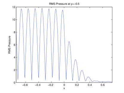
Fig. 6: Snapshot of RMS pressure distribution in space in the sonic crystal along a slice.

3.2 Nonlinear Elasticity in a Spatially Varying Medium

In this section we consider a more difficult test involving nonlinear wave propagation and many material interfaces. This problem was considered previously in [20] and studied extensively in [21]. Solitary waves were observed to arise from the interaction of nonlinearity and an effective dispersion due to material interfaces in layered media.

Elastic compression waves in one dimension are governed by the equations

$$\epsilon_{t}(x,t)-u_{x}(x,t) =0$$ (46a)

$$(\rho(x)u(x,t))_{t}-\sigma(\epsilon(x,t),x)_{x} =0.$$ (46b)

where $\epsilon$ is the strain, $u$ the velocity, $\rho$ the density, and $\sigma$ the stress. This is a conservation law of the form (1), with

$$q(x,t) =\left(\begin{array}[]{c}\epsilon\\ \rho(x)u\end{array}\right) f(q,x) =\left(\begin{array}[]{c}-u\\ -\sigma(\epsilon,x)\end{array}\right).$$

Note that the density and the stress-strain relationship vary in $x$. The Jacobian of the flux function is

$$f^{\prime}(q)=\left(\begin{array}[]{cc}0&-1/\rho(x)\\ -\sigma_{\epsilon}(\epsilon,x)&0\end{array}\right).$$

In the case of the linear stress-strain relation $\sigma(x)=K(x)\epsilon(x)$, (46) is equivalent to the one-dimensional form of the acoustics equations considered in the previous section.

We consider the piecewise constant medium studied in [20, 21]:

$$(\rho(x),K(x)) =\left\{\begin{array}[]{cl}(1,1)&\mbox{if }j<x<(j+\frac{1}{2})\mbox{ for some integer }j\\ (4,4)&\mbox{otherwise},\end{array}\right.$$ (49)

with exponential stress-strain relation

$$\sigma(\epsilon,x)=\exp(K(x)\epsilon)-1.$$ (50)

The initial condition is uniformly zero, and the boundary condition at the left generates a half-cosine pulse.

We solve this problem using the $f$-wave solver developed in [20]. Figure 7 shows a comparison of results using Clawpack and SharpClaw on this problem, with 24 cells per layer. The SharpClaw results are significantly more accurate.

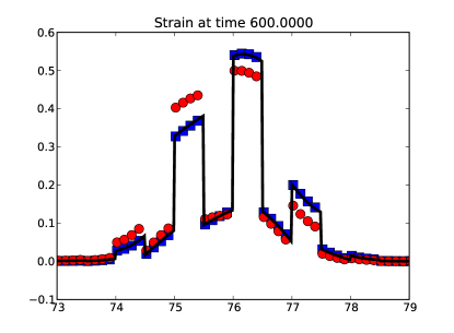
(a) Strain.

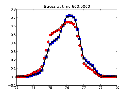
(b) Stress.

Fig. 7: Comparison of Clawpack (red circles) and SharpClaw (blue squares) solution of the stegoton problem using 24 cells per layer. For clarity, only every third solution point is plotted. The black line represents a very highly resolved solution.

Solutions of (46) are time-reversible in the absence of shocks. As discussed in [14, 16], the effective dispersion induced by material inhomogeneities suppresses the formation of shocks, for small amplitude initial and boundary conditions, rendering the solution time-reversible for very long times. This provides a useful numerical test. We solve the stegoton problem numerically up to time $T$, then negate the velocity and continue solving to time $2T$. The solution at any time $2T-t_{0}$, with $t_{0}\leq T$, should be exactly equal to the solution at $t_{0}$. We take $T=600$ and $t_{0}=60$. Figure 8(a) shows the solution obtained using SharpClaw on a grid with 24 cells per layer. The $t=1140$ solution (squares) is in excellent agreement with the $t=60$ solution (solid line). In fact, the maximum point-wise difference has magnitude less than $2\times 10^{-2}$. Using a grid twice as fine, with 48 cells per layer, reduces the point-wise difference to $1\times 10^{-3}$. The Clawpack solution, computed on the same grid (24 cells per layer), is shown in Figure 8(b). Again, the SharpClaw solution is noticeably more accurate. For a more detailed study of this time-reversibility test, we refer to [16].

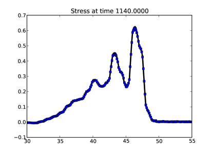
(a) SharpClaw.

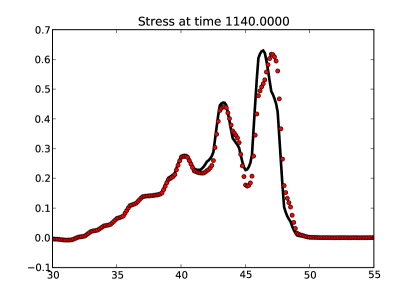
(b) Clawpack.

Fig. 8: Comparison of forward solution (black line) and time-reversed solution (symbols).

3.3 Shallow Water Flow

The next example involves solution of the two-dimensional shallow water equations

$$h_{t}+(hu)_{x}+(hv)_{y} =0$$ (51a)

$$(hu)_{t}+\left(\frac{1}{2}hu^{2}+\frac{1}{2}gh^{2}\right)_{x}+(huv)_{y} =-ghb_{x}$$ (51b)

$$(hv)_{t}+(huv)_{x}+\left(\frac{1}{2}hv^{2}+\frac{1}{2}gh^{2}\right)_{y} =-ghb_{y},$$ (51c)

where $h$, $u$ and $v$ are the depth of the fluid and the velocity components in $x$ and $y$ directions, respectively. The function $b(x,y)$ is the bottom elevation and the constant $g$ represents gravitational acceleration.

Two test cases are presented: a radially symmetric dam-break problem over a flat bottom and a small perturbation of a steady state over a hump. A Roe solver with entropy fix is used in both cases.

3.3.1 Radial dam-break problem

This problem consists in computing the flow induced by the instantaneous collapse of an idealized circular dam. It is widely used to benchmark numerical methods designed to simulate interfacial flows and impact problems.

The domain considered is $[-1.25,1.25]\times[-1.25,1.25]$. The initial depth is

$$h(x,y,t=0) =\begin{cases}2&\mbox{ for }\sqrt{x^{2}+y^{2}}\leq 1/2\\ 1&\mbox{ for }\sqrt{x^{2}+y^{2}}>1/2,\end{cases}$$ (52)

and the initial velocity is zero everywhere. This tests the ability of the method to compute the 2D propagation of nonlinear waves and the extent to which symmetry is preserved in the numerical solution. In the presence of radial symmetry, system (51) can be recast in the following form:

$$h_{t}+(hU)_{r} =-\frac{hU}{r}$$ (53a)

$$(hU)_{t}+\left(\frac{1}{2}hU^{2}+\frac{1}{2}gh^{2}\right)_{r} =-\frac{hU^{2}}{r},$$ (53b)

where $h$ is still the depth of the fluid, whereas $U$ and $r$ are the radial velocity and the radial position. An important feature of these equations is the presence of a source term, which physically arises from the fact that the fluid is spreading out and it is impossible to have constant depth and constant non-zero radial velocity.

A first comparison between SharpClaw and Clawpack is performed by solving the 1D system (53) on the interval $0\leq r\leq 2.5$. A wall boundary condition and non-reflecting boundary condition are imposed at the left and the right boundaries, respectively. The final time for the analysis is taken to be $t=1$. The classical $q$-wave Riemann solver based on the Roe linearization is used to solve the Riemann problem at each interface (see for instance [24] for details), where the left and the right states are computed by using the characteristic-wise WENO reconstruction. The gravitational acceleration is set to $g=1$. A highly resolved solution obtained with Clawpack on a grids with $25,600$ cells is used as a reference solution.

It is well-known that high order convergence is not observed in the presence of shock waves [26] and typically the convergence rate is no greater than first order. However, if we plot the difference between the computed solution available at the cell’s center and the reference solution conservatively averaged on the same grid, i.e. $E_{i}=|Q_{i}-\bar{Q}_{i}|$, then we can visualize where the errors are largest as well as their spatial structure. Figure 9 shows this difference for the water height ($h$) on a grid with $800$ cells. The reference solution at $t=1$ is shown by the solid line in Figure 10. The largest errors in both solutions are near the shocks. In the smooth regions, the SharpClaw solution is more accurate than that of the Clawpack code.

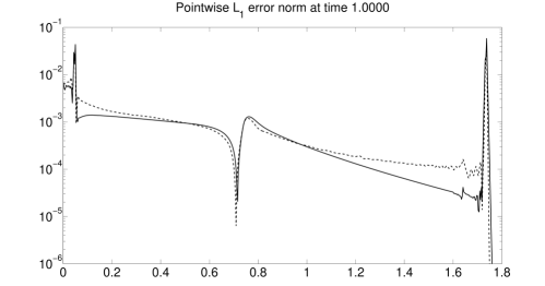
Fig. 9: Pointwise absolute error for the water height on a grid with $800$ cells. Solid line: SharpClaw solution; dashed line: Clawpack solution.

Next we consider the same problem using the full 2D equations (51). The SharpClaw and Clawpack codes are tested on two grids with $125\times 125$ and $500\times 500$ cells. The final time for the analysis is again taken to be $t=1$.

Figure 10 shows the water height $h$ computed with SharpClaw at each cell’s center and $t=1.0$ as a function of the radial position. The radius is measured respect to the center of the initial condition. The 1D reference solution used before is also plotted for comparison. It can be seen that the scheme preserves a good radial symmetry, though it cannot resolve the shock near the origin. The grid is in fact too coarse. Clawpack results are not shown in this figure but indicate similar accuracy and similarly good symmetry.

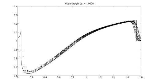
Fig. 10: Solution for the 2D radial dam-break problem on a grid with $125\times 125$ cells, plotted as a function of radius.

The solutions obtained on the finer grid ($500\times 500$ cells) are shown in Figure 11. The effect of the grid refinement is clearly visible. In fact, the solutions gets close to the reference solution. However, the density of the grid near the origin is still too coarse to resolve the shock near the origin to high accuracy.

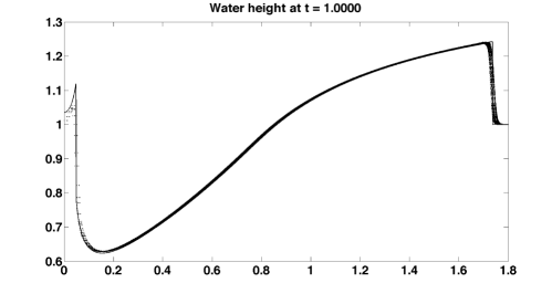
Fig. 11: Solution for the 2D radial dam-break problem on a grid with $500\times 500$ cells, plotted as a function of radius.

3.3.2 Perturbation of a steady state solution

Conservation laws with source terms often have steady states in which the flux gradient are non-zero but exactly balanced by source terms. A good numerical scheme should be able to preserve such steady states and accurately model small perturbations around these conditions. A classical benchmark test case to investigate these properties is the small perturbation of a 2D steady state water given by LeVeque [23].

System (51) is solved in a rectangular domain $[0,2]\times[0,1]$, with a bottom topography characterized by an ellipsoidal gaussian hump:

$$b(x,y)=0.8\exp(-5(x-0.9)^{2}-50(y-0.5)^{2}).$$

The surface is initially flat with $h(x,y,0)=1-b(x,y)$ except for $0.05<x<0.15$, where $h$ is perturbed upward by $\epsilon=0.01$. The initial discharge in both direction is zero, i.e. $hu(x,y,0)=hv(x,y,0)=0$. Non-reflecting (i.e., zero-extrapolation) conditions are imposed at all boundaries. The gravitational acceleration is set to $g=9.81$.

An effort was made to achieve a well-balanced scheme using the $f$-wave approach combined with component-wise or characteristic-wise WENO reconstruction, but this was unsuccessful. This is not surprising, since the algorithm begins by reconstructing a non-constant function. Figure 12(a) shows the contour levels of the solution at $t=0.12$ on a fine grid with $600\times 300$ cells, obtained with the $f$-wave Riemann solver and the component-wise reconstruction approach as a building block for the WENO scheme. The scheme is not well-balanced and spurious waves are generated around the hump. Similar results are obtained using characteristic-wise reconstruction.

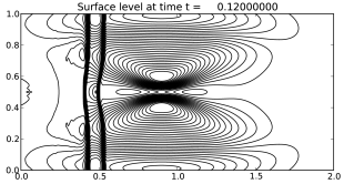
(a) Component-wise reconstruction.

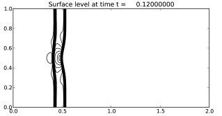
(b) $f$-wave-slope reconstruction.

Fig. 12: Contour of the surface level $h+b$ at time $t=0.12$ computed with component-wise reconstruction and $f$-wave-slope reconstruction. Contour levels: $0.99942:0.000238:1.00656$.

In order to balance the scheme, the $f$-wave-slope reconstruction introduced in Section 2.7 is used instead. In this approach, the WENO reconstruction is applied to waves computed by solving the Riemann problem at the cell’s interface with the $f$-wave solver. The bathymetry is approximated by a piecewise-constant function so that its effect is concentrated at the cell interfaces. When the source term is included in these Riemann problems, the resulting waves vanish as shown in Figure 12(b). In Figure 13 the surface level a cross section along $y=0.5$ at time $t=0.06$ computed with both reconstruction approaches (and the $f$-wave Riemann solver) on a uniform mesh with $600\times 300$ is plotted. This comparison illustrates the different nature of the two approaches. The $f$-wave-slope reconstruction method keeps the surface flat, whereas the component-wise reconstruction introduces spurious waves which have an amplitude of the order of the disturbance that we want to resolve.

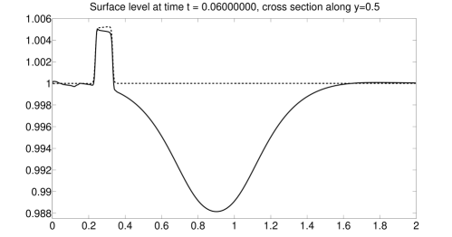
Fig. 13: Surface level $h+b$ along a cross section at $y=0.5$ and time $t=0.06$. Solid line: $f$-wave Riemann solver and component-wise reconstruction; dashed line: $f$-wave Riemann solver and $f$-wave-slope reconstruction.

Figure 14 shows the solution on two uniform meshes with $200\times 100$ cells and $600\times 300$ cells, computed using the $f$-wave-slope reconstruction approach. The results clearly indicate that the detailed structure of the evolution of such a small perturbation is resolved well even with the relatively coarse mesh. These results agree with those reported in [23].

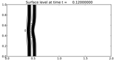
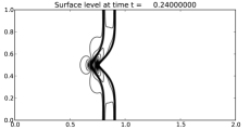
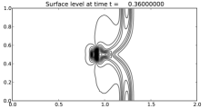
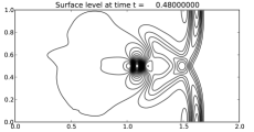
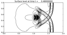
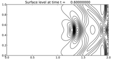
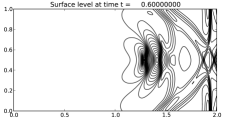
Fig. 14: Contour of the surface level $h+b$. $f$-wave-slope reconstruction. 30 uniformly spaced contour lines. $t=0.12$ from $0.99942$ to $1.00656$; $t=0.24$ from $0.99318$ to $1.01659$; $t=0.36$ from $0.98814$ to $1.01161$; $t=0.48$ from $0.99023$ to $1.00508$; $t=0.6$ from $0.995144$ to $1.00629$. Left: results with a $200\times 100$ cells. Right: results with a $600\times 300$ cells.

In order to investigate the accuracy of our scheme for smooth solutions we also have performed a convergence study at a fixed CFL of 0.3 for the same 2D problem. The smooth initial perturbation is given by

$$h(x,y,t=0)=\exp(-50(x-0.1)^{2})/100$$ (54)

The results of the convergence study are shown in Table 4. A highly resolved numerical simulation computed with Clawpack on a $40,000\times 20,000$ grid has been used as a reference solution. Since the bathymetry $b(x,y)$ is approximated by a piecewise-constant function, both discretizations are formally only second-order accurate, and the results are roughly consistent with this. Nevertheless, the SharpClaw discretization yields significantly more accurate results.

Table 4: Convergence results for the smooth initial condition (54). $L_{2}$-norm of the error as a function of the grid spacing.

	SharpClaw		Clawpack
$\Delta x=\Delta y$	Error	Order	Error	Order
1/10	1.14e-2		2.78e-2
1/20	7.00e-3	0.70	2.09e-2	0.41
1/100	8.11e-4	1.34	6.33e-3	0.74
1/200	3.24e-4	1.32	2.40e-3	1.40
1/1000	2.93e-5	1.49	1.43e-4	1.75
1/2000	5.94e-6	2.30	3.81e-5	1.91

4 Conclusions

We have presented a general approach to extending the finite volume wave propagation algorithm to high order accuracy in one and two dimensions. The algorithm is based on a method-of-lines approach, wherein the semi-discrete scheme relies on high order reconstruction and computation of fluctuations, including a total fluctuation term arising inside each cell. By using WENO reconstruction and strong stability preserving time integration, high order accurate non-oscillatory results are obtained, as demonstrated through a variety of test problems.

This algorithm has several desirable features. Like the second-order wave propagation algorithms in Clawpack [22], it is applicable to hyperbolic PDEs including linear nonconservative systems and nonlinear systems with spatially varying flux function. It has been shown to achieve high order accuracy even for problems with discontinuous coefficients. Finally, the algorithm can be adapted to give a well-balanced scheme for balance laws by use of the $f$-wave approach and a new wave-slope reconstruction technique.

Hyperbolic systems of equations with both smooth and non-smooth solution have been used to test the properties and the capabilities of the proposed method. The schemes have been compared for linear acoustics and nonlinear elasticity problems in heterogeneous media and for the shallow water equations with and without bottom topography. Two types of Riemann solver have been used, i.e the classical ($q$-) wave algorithm and the $f$-wave approach. The new scheme performed well for all the test cases. It gives significantly better accuracy than Clawpack (on the same grid) for smooth problems.

A drawback of our implementation of well-balancing is that it requires the effect of the source term to be approximated entirely at the cell interfaces. For shallow water equations with smooth bathymetry, this will reduce the formal accuracy to second order. Future work might explore the implementation of higher order accurate well-balancing for polynomial source terms using high order quadrature. In any case, in two dimensions, the presented dimension-by-dimension reconstruction approach is formally only second-order accurate (see [34]); however, it gives improved accuracy over the second-order scheme implemented in Clawpack for the test problems considered. Further investigation of different approaches to multidimensional reconstruction for problems containing both shocks and rich smooth flow structures is a topic of future research.

Acknowledgments

The authors are grateful to anonymous referees whose suggestions improved this paper. This work was supported in part by NSF grants DMS-0609661 and DMS-0914942.

References

- [1] N. Ahmad, The f-wave Riemann solver for meso- and micro-scale flows. AIAA Paper 2008-465, 2008.
- [2] N. Ahmad and J. Lindeman, Euler solutions using flux-based wave decomposition, Int. J. Numer. Meth. Fluids, 54 (2006), pp. 47–72.
- [3] D. S. Bale, R. J. LeVeque, S. Mitran, and J. A. Rossmanith, A wave propagation method for conservation laws and balance laws with spatially varying flux functions, SIAM Journal on Scientific Computing, 24 (2002), pp. 955–978.
- [4] M. Castro, J. Gallardo, J. López-GarcÍa, and C. Parés, Well-Balanced High Order Extensions of Godunov’s Method for Semilinear Balance Laws, SIAM Journal on Numerical Analysis, 46 (2008), p. 1012.
- [5] M. J. Castro, P. G. LeFloch, M. L. Munoz, and C. Parés, Why many theories of shock waves are necessary: convergence error in formally path-consistent schemes, J. Comput. Phys., 227 (2008), pp. 8107–8129.
- [6] M. J. Castro Díaz, T. C. Rebollo, E. D. Fernández-Nieto, and C. Parés, On well-balanced finite volume methods for nonconservative nonhomogeneous hyperbolic systems, SIAM Journal on Scientific Computing, 29 (2007), pp. 1093–1126.
- [7] J.-F. Colombeau, A. Y. LeRoux, A. Noussair, and B. Perrot, Microscopic profiles of shock waves and ambiguities in multiplications of distributions, SIAM J. Numer. Anal., 26 (1989), pp. 871–883.
- [8] G. Dal Maso, P. G. LeFloch, and F. Murat, Definition and weak stablity of nonconservative products, J. Math. Pures Appl., 74 (1995), pp. 483–548.
- [9] M. Dumbser, M. Castro, C. Parés, and E. F. Toro, ADER schemes on unstructured meshes for nonconservative hyperbolic systems: Applications to geophysical flows, Computers & Fluids, 38 (2009), pp. 1731–1748.
- [10] T. R. Fogarty, High-Resolution Finite Volume Methods for Acoustics in a Rapidly-Varying Heterogeneous Medium, PhD thesis, University of Washington, 1998.
- [11] T. R. Fogarty and R. J. LeVeque, High-resolution finite-volume methods for acoustic waves in periodic and random media, Journal of the Acoustical Society of America, 106 (1999), pp. 17–28.
- [12] A. Harten, P. D. Lax, and B. van Leer, On upstream differencing and Godunov-type schemes for hyperbolic conservation laws, SIAM Review, 25 (1983), pp. 35–61.
- [13] D. I. Ketcheson, Highly efficient strong stability preserving Runge-Kutta methods with low-storage implementations, SIAM Journal on Scientific Computing, 30 (2008), pp. 2113–2136.
- [14] D. I. Ketcheson, High order strong stability preserving time integrators and numerical wave propagation methods for hyperbolic PDEs, PhD thesis, University of Washington, Seattle, 2009.
- [15] D. I. Ketcheson and R. J. LeVeque, WENOCLAW: A higher order wave propagation method, in Hyperbolic Problems: Theory, Numerics, Applications: Proceedings of the Eleventh International Conference on Hyperbolic Problems, S. Benzoni-Gavage and D. Serre, eds., Berlin, 2008, Springer-Verlag, p. 1123.
- [16] D. I. Ketcheson and R. J. LeVeque, Shock dynamics in layered periodic materials, Communications in Mathematical Sciences, 10 (2012), pp. 859–874.
- [17] D. I. Ketcheson, K. T. Mandli, A. Ahmadia, A. Alghamdi, M. Quezada, M. Parsani, M. G. Knepley, and M. Emmett, Pyclaw: Accessible, extensible, scalable tools for wave propagation problems, SIAM Journal on Scientific Computing, 34 (2012), pp. C210–C231.
- [18] B. Khouider and A. J. Majda, A non-oscillatory balanced scheme for an idealized tropical climate model, Theor. Comput. Fluid Dyn., 19 (2005), pp. 331–354.
- [19] P. G. LeFloch and A. E. Tzavaras, Representation of weak limits and definition of non-conservative products, SIAM J. Math. Anal., 30 (1999), pp. 1309–1342.
- [20] R. LeVeque, Finite-volume methods for non-linear elasticity in heterogeneous media, IJNMF, 40 (2002), pp. 93–104.
- [21] R. LeVeque and D. Yong, Solitary waves in layered nonlinear media, SIAM Journal on Applied Mathematics, 63 (2003), pp. 1539–1560.
- [22] R. J. LeVeque, Wave propagation algorithms for multidimensional hyperbolic systems, Journal of Computational Physics, 131 (1997), pp. 327–353.
- [23] R. J. LeVeque, Balancing source terms and flux gradients in high-resolution Godunov methods: the quasi-steady wave-propagation algorithm, Journal of Computational Physics, 146 (1998), pp. 346–365.
- [24] R. J. LeVeque, Finite Volume Methods for Hyperbolic Problems, Cambridge University Press, 2002.
- [25] R. J. LeVeque and M. J. Berger, Clawpack Software version 4.5, 2011.
- [26] A. Majda and S. Osher, Propagation of error into regions of smoothness for accurate difference approximations to hyperbolic equations, Communications on Pure and Applied Mathematics, 30 (1977), pp. 671–705.
- [27] T. Miyashita, Sonic crystals and sonic wave-guides, Meas. Sci. Technol, 16 (2005), pp. R47–R63.
- [28] M. R. Norman, R. D. Nair, and F. H. M. Semazzi, A low communication and large time step explicit finite-volume solver for non-hydrostatic atmospheric dynamics, J. Comput. Phys., 230 (2010), pp. 1567–1584.
- [29] J. Qiu and C.-W. Shu, On the construction, comparison, and local characteristic decomposition for high-order central WENO schemes, Journal of Computational Physics, 183 (2002), pp. 187 – 209.
- [30] L. Sanchis, F. Cervera, J. Sanchez-Dehesa, J. V. Sanchez-Perez, C. Rubio, and R. Martinez-Sala, Reflectance properties of two-dimensional sonic band-gap crystals, J. Acoust. Soc. Am., 109 (2001), pp. 2598–2605.
- [31] C. Shu, High order weighted essentially nonoscillatory schemes for convection dominated problems, SIAM Review, 51 (2009), p. 82.
- [32] J. B. Snively and V. P. Pasko, Breaking of thunderstorm-generated gravity waves as a source of short-period ducted waves at mesopause altitudes, Geophys. Res. Lett., 30 (2003), p. 2254 doi:10.1029/2003GL018436.
- [33] V. A. Titarev and E. F. Toro, ADER: Arbitrary High Order Godunov Approach, Journal of Scientific Computing, 17 (2002), pp. 609–618–618.
- [34] R. Zhang, M. Zhang, and C.-W. Shu, On the order of accuracy and numerical performance of two classes of finite volume WENO schemes, Communications in Computational Physics, 9 (2011), pp. 807–827.