Glass to superfluid transition in dirty bosons on a lattice

Abstract

We investigate the interplay between disorder and interactions in a Bose gas on a lattice in presence of randomly localized impurities. We compare the performance of two theoretical methods, the simple version of multi-orbital Hartree–Fock and the common Gross–Pitaevskii approach, showing how the former gives a very good approximation to the ground state in the limit of weak interactions, where the superfluid fraction is small. We further prove rigorously that for this class of disorder the fractal dimension of the ground state $d^{*}$ tends to the physical dimension in the thermodynamic limit. This allows us to introduce a quantity, the fractional occupation, which gives insightful information on the crossover from a Lifshits to a Bose glass. Finally, we compare temperature and interaction effects, highlighting similarities and intrinsic differences.

1 Introduction

The physics of disordered quantum systems is a very active field of research since the 1950s, when this topic received the fundamental contributions of Anderson and Mott [1]. Their works showed that, in presence of disorder, even ideal conductors undergo a phase transition towards an insulating state due to destructive quantum interference. An ideal playground for the investigation of quantum effects is offered by ultracold atoms, where a controllable amount of disorder may be implemented in many ways, e.g., by means of speckle potentials, bichromatic lattices with incommensurate frequencies, localized impurities, or site-resolved addressing in optical lattices. After a long search, Anderson localization of ultracold ideal gases was finally observed in one dimension (1D) [2], and very recently reported also in 3D [3].

At this point it is important to stress the fundamental difference between disordered fermionic and bosonic systems. For fermions the crucial role is played by the Fermi energy: the question whether a given system is a conductor or insulator depends on whether the single particle states close to Fermi level are localized or not. Bosons, in contrast, tend to condense in the lowest energy state (or states). The question whether they constitute a superfluid or an insulator reduces then to understanding if the low-energy states are localized or not (for more extensive discussion see for instance [4, 5]).

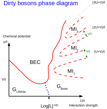
Figure 1: Schematic phase diagram for dirty bosons at zero temperature as a function of interactions ($U$) and chemical potential ($\mu$) containing glassy (G), superfluid (BEC), and Mott insulating (MI) phases. The continuous and dashed lines mark respectively the superfluid-insulator and glass-Mott transition, while the dotted line indicates a crossover from the Lifshits glass (heavily fragmented) to the Bose glass (extended) region. Outside of the BEC region, the one-body density matrix $\rho({\bf r},{\bf r^{\prime}})$ decays as $|{\bf r-r^{\prime}}|\to\infty$. The Mott insulator lobes appear at sufficiently strong interactions, as the inclusion theorem guarantees that there may be no MI for $U<V$.

In the past decades there appeared an enormous literature on disordered systems, see, e.g., [6, 7, 8, 9, 10, 11, 12, 13, 4, 14, 5], although due to the complexity of the topic mathematically rigorous results are still scarce. A great deal of work has been done on random Schrödinger operators, which describe single particle behaviour, see [15] for an excellent survey. In the recent paper [16] two of us have provided rigorous tight bounds on the ground state energy, as well as approximations of the ground state and excited states wave-functions for the case of random impurity (Bernoulli) disorder in a 1D lattice. Since in this case the shape of the low-energy states is known, there are analytical ways to estimate interaction energy and obtain rigorous results also for interacting systems.

A challenging and still open problem is the understanding of interaction effects on disordered systems. A crucial step forward in our understanding of dirty bosonic systems was made by Giamarchi and Schulz [6] and Fisher et al. [7] who conjectured that, in presence of weak disorder, interactions give rise to an intermediate compressible but insulating phase, the Bose glass, in between the superfluid and the insulating strongly-interacting phases (Tonks gas in continuous 1D systems, or Mott insulator in lattice systems). The disputed controversy, as to whether or not the insulating Mott phase is always surrounded by a glassy phase was finally settled in [13], who demonstrated, using the theorem of inclusions, that this is indeed the case for the dirty boson system with generic bounded disorder. Experimentally, this problem has been recently addressed in [17, 18, 19].

In the regime where disorder dominates over interactions, it was shown instead that the ground state of the quantum fluid may be described in terms of a qualitatively different glassy phase, called Lifshits (or Anderson) glass [10, 20], characterized by exponentially localized and well separated ”islands”. The latter may be identified with the low-lying single-particle eigenstates residing in the regions of space where the potential is small. As repulsive interactions are strengthened, an increasing number of islands is populated, until their overlap becomes sufficient to establish phase coherence and transport between them. The gas as a whole then undergoes a phase transition towards an extended Bose–Einstein condensate (BEC). If the gas is confined in a lattice, for even larger interactions the repulsion between particles becomes so strong that on-site density fluctuations characteristic of the superfluid state become energetically unfavourable. In this situation the gas undergoes a further transition out of the BEC, first to the Bose glass phase and then into the incompressible Mott state. Between the Lifshits and the Bose glasses there is no phase transition, as both are gapless, insulating and compressible phases, but nonetheless the two states are qualitatively different, in the sense that in the former the gas is fragmented into independent and distant low-energy islands (the Lifshits states), while the latter tends to extend over a large portion of the available volume. The phases discussed above are sketched in figure 1, and their most important properties listed in table 1.

Table 1: Summary of most common phases for dirty bosons in a lattice, and associated properties.

• 		Superfluid	Compressible	Gapless	Fragmented
  BEC		Y	Y	Y	N
  Glass	Lifshits	N	Y	Y	Y
  	Bose	N	Y	Y	N
  Mott insulator		N	N	N	N

In the present paper we consider disorder of Bernoulli type, i.e., randomly-distributed, identical and localized impurities, and we focus on the regime of weak to intermediate interactions in presence of such impurities. We first investigate the properties of the ideal gas, discussing the typical size and energy of the localized islands, and showing that the low-energy states indeed form a so-called Lifshits tail.

We further explore interaction effects on the ground state properties by comparing the performance of two theoretical methods. The first one is a simple version of the multi-orbital Hartree–Fock method (sMOHF), a variational method based on an expansion on single-particle states. This approximation is appropriate to describe the glassy regime where superfluidity is suppressed by disorder [10]. More elaborate versions of the Hartree–Fock method, that incorporate self-consistency and allow to describe fragmentation and quantum dynamics of interacting Bose systems can be found in [21] and references therein. The second method is the standard Gross–Pitaevskii (GP) approach, which generally yields an appropriate description for every interaction strength.

We calculate the ground state energy of the system, the associated superfluid fraction, the fractal dimension, and introduce a new parameter, the fractional occupation, allowing one to discern between the Lifshits and the Bose glass. Finally, we turn to the investigation of temperature effects in an ideal gas. Due to the increase of kinetic energy, temperature yields effects similar to those generated by repulsive interactions, in the sense that the gas occupies a larger number of islands, which increasingly overlap until the ground state covers a large amount of the available space. Nonetheless, we will point out that there are important differences between the two cases.

As an important result, in this paper we show that disordered systems with Bernoulli potential allow for analytical estimates which are very well supported by numerical simulations. These results provided us with intuitions on how to generalize the rigorous results of [16] to non-interacting 2D systems, and, at least partially, to interacting 1D and 2D systems. These rigorous results go beyond the scope of the present article, and will be published in a more appropriate mathematical physics journal.

This paper is structured as follows. We introduce the disordered potential under study and the relevant Hamiltonian in Sec. 2. In Sec. 3 we identify the eigenstates of the ideal system, we numerically demonstrate the Lifshits tail behaviour, and we discuss the ground state energy scaling as a function of the size of the system. In Sec. 4 we introduce the sMOHF and GP methods, and in Sec. 5 we compute a number of relevant quantities for interacting systems. In Sec. 6 we compare the effects of interactions and non-zero temperature, and we present our conclusions in Sec. 7.

2 The model

We study the properties of a bosonic gas on disordered 1D and 2D square lattices of linear dimension $L$. We consider disorder of the so-called Bernoulli type, i.e., the potential on each site is an independent random variable that assumes the value:

$$V_{i}=\left\{\begin{array}[]{ll}V>0&{\rm with\,probability\,}1-p\\ 0&{\rm with\,probability\,}p\\ \end{array}\right.$$ (1)

This kind of potential may be ideally realized by using a two-component gas, and a species-selective lattice which deeply traps only one of the two components [22, 19]. At sufficiently low energies, the component which is not trapped experiences $s$-wave collisions against localized scatterers. Alternatively, a Bernoulli disorder may be imprinted directly on the gas exploiting single-site addressable optical lattices [23].

The use of Bernoulli disorder is particularly appealing because its asymptotic properties, as discussed in the next sections, become apparent even for small lattices (e.g., with $50^{D}$ sites). As we show in A, the Bernoulli potential has actually optimal properties of convergence. Therefore, the Bernoulli disorder is suitable for numerical simulations and due to its simple form, it allows for various analytical estimates.

The Hamiltonian of the interacting system we consider is then

$$\hat{H}=-t\sum_{\langle i,j\rangle}\hat{c}_{i}^{\dagger}\hat{c}_{j}+\sum_{i}V_{i}\hat{c}_{i}^{\dagger}\hat{c}_{i}+\hat{U}_{\rm int},$$ (2)

where $t$ denotes the tunnelling energy, $\hat{c}_{i}^{\dagger}$ is the creation operator of bosons on site $i$, and $\langle i,j\rangle$ denotes nearest neighbour pairs of sites. The interaction term $\hat{U}_{\rm int}$ will be discussed later in Section 4.

3 Properties of a non-interacting gas

Let us start by discussing the properties of a non-interacting system, and in particular look at its ground state energy, and the density of low energy excited states.

3.1 Ground state energy

In a large 1D system with Bernoulli disorder, the linear size $L_{\rm max}^{\rm(1D)}$ of the largest island of contiguous zero-potential sites scales as $L_{\rm max}^{\rm(1D)}\propto\log L$ [16]. The proof of this fact is based on the following simple observation. Let $l_{0}$ be the characteristic size of the largest island, then $p^{l_{0}}$ estimates its occurrence. The number of islands of similar size is expected to be of order of $L$ (strictly speaking $L/\log{L}$ as we shall discuss below), so that the probability of occurring of any one of them is $Lp^{l_{0}}\to{\rm const}$ as $L\to\infty$, which indeed implies $l_{0}\simeq\log{L}/|\log(p)|$. It is then clear that the ground state energy of the non-interacting bosonic gas in such a potential will be bounded above by the energy of the first harmonic, i.e., a half-sine function, of the largest island. A lower bound of the same order was proven in [16], showing that the ground state energy behaves asymptotically as $\pi^{2}/(\log L)^{2}$ when $L\to\infty$.

Similarly, one can argue that in a large D-dimensional system the ground state will be occupying the largest spherical island of zero-potential sites since this shape minimizes the kinetic energy [24]. Its diameter can be shown to grow as $L_{\rm max}^{\rm(D)}\propto(\log L)^{1/D}$, and therefore we expect the energy of the ground state to scale as $E_{0}\propto\log L^{-2/D}$. Again, the proof is based on the similar argument as in the 1D case, except that one has to replace the characteristic length $l_{0}$ by the volume $l_{0}^{D}$ in arbitrary dimension. The numerical confirmation of the scaling for the 2D case is shown in the inset of figure 2.

For comparison, we plot in the same inset the ground state energy obtained from a random-amplitude disorder (i.e., one where to each site corresponds a random potential $V_{i}$, uniformly distributed in the interval $[0,V^{{}^{\prime}}]$). We see that the rate of convergence of the energy for a Bernoulli distribution is quicker than for a uniform distribution. Because of this, the potential with a Bernoulli distribution is ideal for ground state energy convergence as well as localization of low energy states. This may be quickly seen as follows, while further details are given in A. If the potential takes value zero with a positive probability $p$, one can define islands of zero potential as the natural locus of the ground eigenstate. In cases where the values of the potential are positive, even when they are arbitrarily close to zero, the low potential islands can still be defined, using a (volume-dependent) energy cut-off, but the contribution to energy from such islands will in this case be larger. Accordingly, the convergence of the ground state energy to zero will be faster in the former case. Among the distributions which assign a fixed probability $p$ to the zero value of the potential, the optimal ones to work with are the Bernoulli distributions, in which some positive value $V$ is assumed with probability $1-p$. While the rate of convergence of the ground state energy to zero is comparable for all such distributions, the advantage of the Bernoulli distribution is that it localizes the low energy states more clearly. The analysis of other potential distributions is more complicated, because it necessitates introducing an energy cut-off to define low potential islands. The Bernoulli potential is also easier to work with numerically, since it requires sampling fewer potential realizations.

Although we do not expect any of the properties discussed in the following to depend on the specific type of bounded disorder, we clearly see that the Bernoulli choice yields a much faster convergence of the ground state energy to the desired asymptotic behaviour.

3.2 Lifshits tail

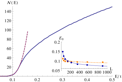
Figure 2: Properties of non-interacting dirty bosons in 2D. Main figure: the cumulative density of states $\mathcal{N}(\epsilon)$ shows a Lifshits tail (purple dashed line) given by (3). Here we have taken a 200$\times$200 lattice, and averaged over 10 realizations. Inset: ground state energy $E_{0}$ in 2D plotted versus linear size of the system $L$; results for Bernoulli disorder are plotted in blue and scale as $\sim 1/\log L$, while results for random-amplitude disorder are plotted in orange and scale as $\sim\log\log L/\log L$.

Since the disordered potential is chosen to be finite, the spectrum of the system is bounded from below. As a consequence, the spectrum is expected to exhibit a so-called Lifshits tail [10, 25], in the sense that the cumulative density of states (cDOS) $\mathcal{N}(\epsilon)=\int^{\epsilon}\mathrm{d}\epsilon^{\prime}\ \mathcal{D}(\epsilon^{\prime})$ behaves at low energies as

$$\mathcal{N}(\epsilon)\sim\exp\left[-c(\epsilon-V_{\rm min})^{-D/2}\right].$$ (3)

The cDOS and the associated Lifshits tail for the considered 2D system were obtained numerically and are shown in figure 2. The Lifshits states lie on well-separated islands, and have almost degenerate energies since the islands’ diameters are approximately the same.

4 Interacting case

In this Section we will present two common theoretical approaches used to describe a Bose gas with short-range interaction potential. The first one corresponds to a simplified version of Multi-Orbital Hartree–Fock (sMOHF) method, based on an expansion into single-particle eigenstates. As we will see, sMOHF is suitable to describe a weakly-interacting system, whose ground state occupies few disconnected large islands of zero potential. For more sophisticated version of the Hartree–Fock approach applied to bosons, see [21]. The second method is the standard Gross–Pitaevskii (GP) equation, which describes the dynamics of a fully-coherent matter wave, and correctly describes also the regime of strong interactions, where large overlaps between the islands and self-interaction on each island play an important role. overlap between the islands.

Before going into details, let us estimate when the sMOHF description based on non-interacting single particle states should be valid. As we have discussed, this regime corresponds to the Lifshits glass region. Let us assume that we have $\tilde{r}$ filled islands of the characteristic size $l_{0}$, and ”volume” $l_{0}^{D}$, so that

$$\tilde{r}l_{0}^{D}=CL^{D},$$

where the proportionality constant $C$ depends, in general, weakly on $p$ and the density $\rho$, since it results from the complex interplay between the kinetic and interaction energy. In the following we will ignore this dependence.

The Lifshits glass regime occurs then for an inter-particle interaction coupling $g$ smaller than the characteristic value $g_{\rm ch}$, at which the kinetic energy is comparable to the interaction energy. An estimate of the characteristic coupling is easily obtained by equating the kinetic energy per particle $\simeq 1/l_{0}^{2}$, with the interaction energy $\simeq gN/\tilde{r}l_{0}^{D}$. Using the above expression for $\tilde{r}$, we obtain

$$g_{\rm ch}\simeq C/\rho l_{0}^{2}\simeq C(|\log{p}|)^{2/D}/\rho(|\log{L}|)^{2/D}.$$ (4)

This scaling provides a good estimate of the coupling at which the two energies depicted in figure 3 start to diverge.

4.1 Multi-orbital Hartree–Fock approach

In the sMOHF treatment, the wave function is expressed in the single particle eigenstates, and is taken to be in the product form

$$|\Psi\rangle=\prod_{k}\frac{(\hat{a}^{\dagger}_{k})^{n_{k}}}{\sqrt{n_{k}!}}|0\rangle,$$ (5)

where $|0\rangle$ is the vacuum of the system and $a^{\dagger}_{k}$ creates a particle in the $k$th non-interacting eigenstate (i.e., orbital). We consider repulsive interactions of strength $g>0$, which yield an interaction energy given by

$$\langle\hat{U}_{\rm int}\rangle=\frac{g}{2}\int\rm{d}{\bf x}\ \hat{\psi}^{\dagger}({\bf x})\hat{\psi}^{\dagger}({\bf x})\hat{\psi}({\bf x})\hat{\psi}({\bf x})=$$

$$\frac{g}{2}\int\rm{d}{\bf x}\sum\psi^{*}_{k_{1}}({\bf x})\psi^{*}_{k_{2}}({\bf x})\psi_{k_{3}}({\bf x})\psi_{k_{4}}({\bf x})\hat{a}^{\dagger}_{k_{1}}\hat{a}^{\dagger}_{k_{2}}\hat{a}_{k_{3}}\hat{a}_{k_{4}},$$ (6)

where the sum runs only over terms conserving number of particles, i.e., such that $k_{1}+k_{2}=k_{3}+k_{4}$. The diagonal terms ($\hat{a}^{\dagger}_{k}\hat{a}^{\dagger}_{k}\hat{a}_{k}\hat{a}_{k}$) contribute a factor $\frac{g}{2}\sum_{k}{n}_{k}({n}_{k}-1)O_{k,k}$, where we have defined the overlaps $O_{k,j}=\int{\rm d}{\bf x}|\psi_{k}({\bf x})|^{2}|\psi_{j}({\bf x})|^{2}$.

There are two other possibilities which conserve the number of particles: ($k_{4}=k_{1}$ and $k_{3}=k_{2}$), or ($k_{4}=k_{2}$ and $k_{3}=k_{1}$). These two terms, called direct and exchange terms, are equal for bosons, and their sum contributes a factor $\frac{g}{2}\sum_{j\neq k}2n_{k}n_{j}O_{k,j}$.

The average interaction energy reads then:

$$\langle\hat{U}_{\rm int}\rangle=\frac{g}{2}\sum_{k}\left[n_{k}(n_{k}-1)O_{k,k}+\sum_{j\neq k}2n_{k}n_{j}O_{k,j}\right].$$ (7)

The occupation probabilities $n_{k}$ yielding the ground state may now be found by minimizing the total energy

$$E=\sum_{k}n_{k}E_{k}+\langle\hat{U}_{\rm int}\rangle,$$ (8)

subject to the constraints of normalization and positivity of all $n_{k}$,

$$\sum_{k}n_{k}=N,\quad\forall k,\,n_{k}\geq 0.$$ (9)

We present the analytic solution of this problem in B.

4.2 Gross–Pitaevskii approach

The properties of the system may be analysed also in the framework of the usual GP equation,

$$\left(-\frac{\hbar^{2}}{2m}\triangle+V+gN|\psi({\bf x})|^{2}\right)\psi({\bf x})=\mu\psi({\bf x})$$ (10)

which describes the behaviour of an interacting Bose gas in terms of a single-particle coherent wave-function. We find the ground state and the chemical potential $\mu$ by imaginary time evolution, applying an operator split method. The ground state energy $E$ is related to $\mu$ by the formula

$$E=\mu-\frac{gN}{2}\int\rm{d}{\bf x}\,|\psi({\bf x})|^{4}.$$ (11)

5 Comparison of $\mathbf{sMOHF}$ and GP approaches

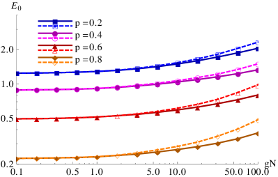
Figure 3: Ground state energies obtained by sMOHF (dashed) and GP (continuous) for various disorder densities $p$. The value of the coupling constant at which the energies obtained by the two methods start to diverge is estimated by equation (4). Results obtained by averaging over 5 simulations and $V=5t$.

In this Section, we present the numerical solutions of the sMOHF and GP equations, comparing the performance of the two methods. In particular, we discuss and compare the ground state energy, the superfluid fraction, and the fractal dimension. As we will see, in the regime of strong disorder (Lifshits regime) sMOHF provides ground state energies in accord with GP. Nonetheless, sMOHF has the advantage of being insensitive to convergence issues, and its solution is generally much faster than GP. The fact that in this regime both methods agree confirms the intuition that the particles populate low-lying eigenstates, the Lifshits islands. In the regime where interactions dominate over the disorder, we will show instead that GP provides energies which are perceptibly lower than sMOHF. Unless otherwise noted, the numerics presented in this section have been obtained for a system on a 2D lattice with $32\times 32$ sites, $N_{\mathrm{part}}=10^{4}$ particles, a Bernoulli potential with $V=5t$ or $V=50t$, and we have set $t=\hbar^{2}/2m=k_{B}=1$. Where needed, we have performed appropriate averages to obtain results which are independent of the particular disorder configuration.

5.1 Energy

In figure 3 we compare the energies obtained through the sMOHF approach with those obtained from the GP equation as a function of the interaction strength $g$. For a coupling constant $g$ smaller than a characteristic value $g_{\rm ch}$, the minimization of expression (8) and the GP equation yield the same values of energy proving that sMOHF method correctly describes the system in this limit. The characteristic value $g_{\rm ch}$ is given by the interaction strength at which the energy obtained from the sMOHF starts to differs from the one obtained by the GP equation. The range of $g$ for which sMOHF approach is an equivalent description shrinks with increasing $p$, as the scatterers become increasingly sparser, leaving large regions of zero potential. The range of applicability of sMOHF also shrinks with decreasing $V$. For values of the interaction $g\gg g_{\rm ch}$, the disorder plays a negligible role and the energy per particle saturates to the analytic value $E=\overline{E}+g\rho/2$, where $\overline{E}$ is a constant that depends on $V$ and $p$. This analytic result is recovered by the numerical solution of the GP equation, but not by the sMOHF approach.

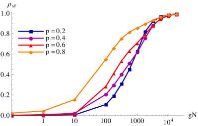
a) b)

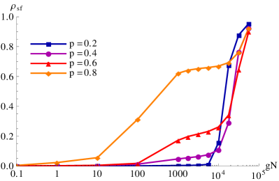
Figure 4: Superfluid fraction $\rho_{\rm sf}$ as a function of potential density $p$ and interaction strength $g$ for a) $V=5t$ b) $V=50t$.

5.2 Superfluid fraction

The superfluid fraction $\rho_{\rm sf}$ may be defined in terms of the energy change of a periodic system in response to twisted boundary conditions along one direction. To calculate this quantity we solve the GP equation (10) with boundary conditions $\psi_{i+L,j}={\rm e}^{{\rm i}\Phi}\psi_{i,j}$, and we obtain

$$\rho_{\rm sf}=\frac{2mL^{2}}{\hbar^{2}}\frac{E(\Phi)-E(0)}{\Phi^{2}},$$ (12)

where $E(\Phi)$ is the energy per particle of a system with the total phase shift $\Phi$. Our results are depicted in figure 4. In the regime where sMOHF provides a good description, the SF fraction is negligible because the localized single-particle eigenstates experience an exponentially small energy change due to the imposed phase shift. The GP equation instead yields a perceptibly lower energy than sMOHF when the superfluid fraction $\rho_{\rm sf}$ becomes sufficiently large ($\rho_{\rm sf}\gtrsim 0.1$).

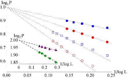
Figure 5: Scaling of the logarithm of the participation number $\log_{L}P$ versus the inverse of the logarithm of the lattice size. The slope of the lines, being the logarithm of $c$, allows for determining the fraction of space occupied by the state. Main figure: 1D lattice of length $L$, and interaction strengths $g=0.1$(empty) and $g=10$(filled). The potential densities are respectively $p=0.4$(red circles) and $0.7$(blue squares). Inset: 2D lattice of linear size $L$, interaction strength $g=10$, potential parameter $p=0.6$(green diamonds), $0.8$ (purple triangles).

5.3 Fractal dimension

As we have discussed in the previous sections, the ground state of a weakly-interacting fluid is localized on one or a few Lifshits islands. When interactions start to play an important role, the extension of the ground state increases generally until the gas occupies all available space. In order to provide a quantitative measure of the extension of the ground state, we calculate its fractal dimension $d^{*}$ [1], and introduce here the concept of fractional occupation $c$.

The fractal dimension is defined as a minimum $d^{*}$ such that

$$\lim_{L\rightarrow\infty}\frac{P}{L^{d^{*}}}=c,\,c>0.$$ (13)

Here $P=1/\int\rm{d}{\bf x}|\psi_{0}({\bf x})|^{4}=1/O_{0,0}$ is the so-called “participation number” of the ground state [1]. For an extended state such as a plane wave one finds that $P$ is proportional to the volume of the system, and therefore the fractal dimension equals the Euclidean dimension, $d^{*}=D$. For a state which is instead localized in a volume $Q$, the participation number behaves as $Q$, and the corresponding fractal dimension vanishes if $Q$ grows slower than any power of $L$. For instance, the ground state of the non-interacting system is localized on an island of volume $Q\sim\log L$ which for all $\alpha$ grows slower then $L^{\alpha}$. So, in general, one has $0\leq d^{*}\leq D$.

Analysing the results obtained from both sMOHF and GP approaches, we find that $d^{*}=D$ for any $g>0$. This may be seen as follows. Assuming that $d^{*}$ is bounded strictly below $D$, we see that the interaction energy $(gN/2)\int\rm{d}{\bf x}\,|\psi_{0}({\bf x})|^{4}$ will diverge. Physically, there is not enough space for the particles to keep the interaction energy bounded unless they spread out through a non-zero proportion of the whole space. If $\log_{L}P=D-f(L)$, and $\lim_{L\to\infty}L^{D}/L^{d^{*}}=c$, then it must be that $L^{f(L)}\to c$, so $f(L)\approx\log(c)/\log(L)$. Numerical results confirm this behaviour in both 1D and 2D. To show this, in figure 5 we plot $\log_{L}P$ as a function of $1/\log L$ for a 1D system and a 2D system (inset).

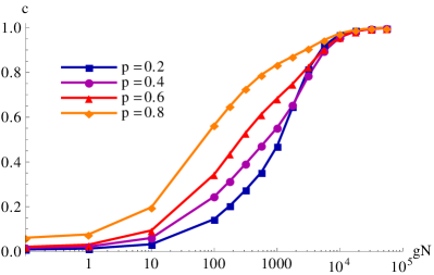
a) b)

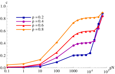
Figure 6: Fractional occupation $c$ of the ground state as a function of potential density $p$ and interaction strength $g$ for a) $V=5t$ and b) $V=50t$. Here we have considered a 2D lattice and $c$ was obtained by averaging over 5 potential realizations.

The quantity $c$, which takes values between 0 and 1, can be interpreted as the fraction of space occupied by the ground state, and we will therefore refer to it as the fractional occupation of the ground state. We show our results for the fractional occupation in figure 6.

For strong disorder ($V\gg t$) the fractional occupation $c$ displays at intermediate interactions a plateau at $\sim p$. This coincides with a similar plateau in the plot of the superfluid fraction (cf. figures 4b and 6b). In 1D the explanation for such behaviour of $c$ and $\rho_{\mathrm{sf}}$ is the following. For small $g$ the wave function fills only a part of zero-potential space. Indeed, for $g=0$, we have a linear operator and therefore the ground state is approximately the wave function on the longest island of zero potential, yielding a nearly zero $c$. For $g$ small such that $gN/2$ is approximately $1/(\log L)^{2}$, the ground state spreads to many of the long islands: the kinetic energy increases a little (on the order $1/(\log L)^{3}$) while interaction energy decreases by a factor $1/(\#$ of islands). As $g$ grows to be on the order of $1$, it supports itself on all sites of zero potential save for the shortest islands, so $c\approx p$. This is where the graphs level off in (Fig 6), where the ground state does not have large norm on short islands of zero potential and sites of $V$ potential.

For large interactions one may use the Thomas-Fermi Approximation, cf. [5]. Suppose we choose an ansatz such that the wave function equals $\frac{m}{\sqrt{pL}}$ on sites of zero potential and $\frac{\sqrt{1-m^{2}}}{\sqrt{qL}}$, then energy optimizing $m$ would be $m^{2}=p+\frac{pqV}{g\rho}$ and $1-m^{2}=q-\frac{pqV}{g\rho}$. If $g\rho\leq pV$, then the above ansatz is invalid, and the ground state stays exclusively on sites of zero potential. If we compare the energy of a wave function equal to $\frac{1}{\sqrt{pL}}$ on sites of zero potential and zero elsewhere to a wave function that is equal to $\frac{1}{\sqrt{L}}$ everywhere, and ignore the kinetic energy terms (which we can control by another parameter), we see that the first wave function provides a better variational ansatz if $\frac{g\rho}{2}\leq pV$. This means that for $g\rho\lesssim 2pV$, we are in an area where $c\approx p$, that is, the kinetic energy and interaction energy are balancing, but any significant support of the ground state on the sites occupied by scatterers is too costly. Since the wave function does not spread significantly in this regime, also the superfluid fraction remains constant.

6 Comparison of temperature and interaction effects

In this section we turn to the analysis of the effects of non-zero temperature in a non-interacting system. We will see that those remind very much effects of interactions at zero temperature, and yet are quite different.

6.1 Single-particle density distribution

For free boson systems, the effects of temperature may be studied by expanding arbitrary states in the basis of non-interacting eigenstates, in analogy with what we did to treat the interacting case. In this approximation, the average density of the gas reads

$$\rho({\bf x})=L^{-D}\sum n_{k}|\psi_{k}({\bf x})|^{2}.$$ (14)

An approximation of a typical wave-function is then given by

$$\psi({\bf x})=\sum\sqrt{w_{k}}{\rm e}^{i\phi_{k}}\psi_{k}({\bf x}),$$ (15)

where ${\rm e}^{i\phi_{k}}$ are random phases, and $w_{k}$ is a Gaussian random variable with distribution $\mathcal{P}(w_{k})=n_{k}^{-1}{\rm e}^{-w_{k}/n_{k}}$, such that $\langle w_{k}\rangle_{\mathcal{P}}=n_{k}$.

The occupation factors depend on the statistics of the particles. Identical bosons follow the Bose–Einstein distribution

$$n_{k}=\frac{1}{{\rm e}^{(E_{k}-\mu)/T}-1}.$$ (16)

Distinguishable (or classical) particles would instead populate the non-interacting eigenstates following a Boltzmann distribution, $n_{k}={\rm e}^{-(E_{k}-\mu)/T}$.

At zero temperature, only the lowest energy state will have a non-zero population, i.e., $n_{k}=N\delta_{0,k}$. Non-zero temperatures will modify the occupation probabilities, redistributing population over the higher energy states, but we expect that for $T\ll t$ only the lowest energy states (the Lifshits states) will be populated.

We note here that in an interacting 2D Bose gas of finite extension one generally expects a crossover between two qualitatively different regimes. At very low temperatures ($T<T_{C}$) phase correlations in the gas decay algebraically with distance. For temperatures larger than the critical value $T_{C}$ instead, phase correlations decay exponentially with distance. This switch in the decay of correlations can be traced back to the dissociation of bound vortex-antivortex pairs at $T>T_{C}$. The crossover becomes a real phase transition in an infinite system, and the underlying mechanism goes under the name of Berezinskii-Kosterlitz-Thouless (BKT) transition [26].

Our approach to finite temperatures is rather crude, and is not well suited to describe BKT physics, which requires considering both temperature and interactions at the same time. However, for the range of parameters considered in this manuscript, our model provides a qualitative, although simplified, explanation of the complementary roles payed by temperature and interactions. Moreover, a similar scenario to the one considered here is present in three dimensions, where a true BEC exists at low temperatures.

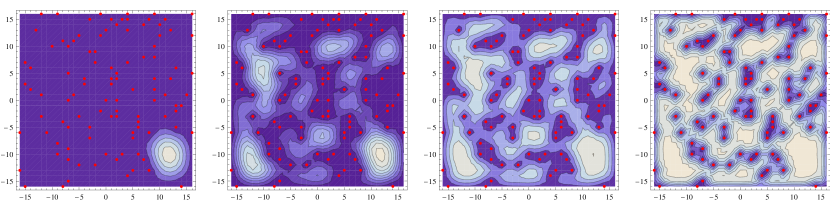
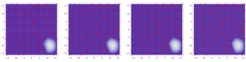
a) b) c)

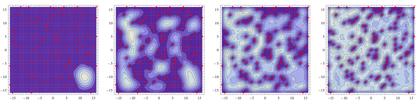
Figure 7: Comparison of temperature and interaction effects. First two rows: thermally averaged single particle density with respectively Boltzmann (top) and Bose (centre) statistics; from left to right, $T/t=$0, 0.1, 0.2, 0.5.
Bottom row: single particle density of an interacting gas; from left to right, $g\rho/t=0,\ 0.1,\ 2,\ 10.$
The red dots indicate the sites occupied by the disordered scatterers. The average density is $\rho=0.9$particles/site.

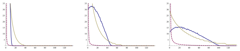
Figure 8: Occupations of the single particle states for the simulations shown in columns 2,3, and 4 of figure 7. The lines are: Boltzmann (yellow dotted), Bose (red dashed), and sMOHF (blue continuous). Results averaged over 200 simulations. x-axis: index labeling the single-particle state; y-axis: occupation.

6.2 Non-zero temperature

As temperature is raised, the cloud gets to occupy more and more islands; when $T\lesssim V$ it will populate all unoccupied sites, and for $T\gg V$ it will occupy even sites inhabited by scatterers.

The averaged densities in presence of positive non-zero temperature are shown in figure 7a) and b). While a classical cloud quickly spreads over various low energy states, a bosonic gas at low temperatures tends to condense in a single or few Lifshits states. Interaction effects in a bosonic cloud at $T=0$, instead, yield at first sight a state which very much resembles the Boltzmann case. Even for moderate repulsive interactions, the cloud spreads over various Lifshits states. Effects of interactions at $T=0$ are shown in figure 7c.

The occupation probabilities $n_{k}$ for the three cases analysed above (Boltzmann, Bose, and interacting) are shown in figure 8. Since the lowest-energy single-particle states correspond to the localized and well separated Lifshits states, a population distribution which is narrow in energy corresponds to a ground state localized on one or very few well-separated islands, the Lifshits glass. As the temperature increases the Bose liquid tends to have a rather narrow population distribution, while the Boltzmann and interacting distributions quickly spread. Nonetheless, a few important differences may be noted comparing the two latter cases, as maybe seen in Figs. 7a and 7c. While the population distribution for the Boltzmann case smoothly decreases, with a long tail, the distribution for the interacting case has a local minimum at very low $k$, while at larger $k$ goes through a maximum and then quickly drops to zero. These features can be understood in the following way. The eigenstates with lowest energies tend to have higher inverse participations (overlaps), i.e., the Lifshits states are rather concentrated on a single or few islands while states at intermediate energies are delocalized over the whole system. For an interacting system is therefore preferable to occupy states indexed by states with intermediate $k$ values, as their larger spatial extension helps to reduce the interaction energy. At very high energies ($k\gg 1$) instead the states have again very high $O_{kk}$, since they become completely localized on single sites, and their populations abruptly drop to zero, as it is too costly energetically to put particles with repulsive interactions in small regions of space.

7 Conclusions

In this paper we have considered a bosonic lattice gas in the presence of Bernoulli disorder, given by randomly-localized identical scatterers. We have shown that in this case it is possible to provide precise analytical estimates even for the interacting case. We have compared two theoretical schemes, the simplified multi-orbital Hartree–Fock and the Gross–Pitaevskii approaches, showing how the first is very accurate in the glassy regime of strong disorder, but it fails when interactions bring the system into an extended state and the superfluid fraction reaches values $\rho_{\it sf}\gtrsim 0.1$.

Further, we have shown analytically that the fractal dimension for this kind of potential tends to the physical dimension of the system. As a result, we have introduced a quantity termed fractional occupation, which characterizes the typical extension of the system. When the latter becomes of order $p$, i.e., the fraction of physical space where scatterers are absent, the system crosses over from the Lifshits to the Bose glass. Finally, we have discussed the similarities and differences between effects due to interaction and temperature. This question is of fundamental importance for ongoing experiments, since in a laboratory the two effects are often difficult to distinguish. We hope that our results will provide new insights in the complex route towards understanding the interplay between disorder, interactions, and temperature in quantum mechanical systems.

Appendix A Comparison of the Bernoulli and uniform distributions

The choice of potential may change the behaviour and scaling of the ground state energy in a single-particle system. We will consider potentials that are bounded below at $0$ and to simplify notation let $P(x)=P[V_{j}\leq x]$ for a given distribution. Any potential that is bounded below can be shifted so that the bottom of its support is zero. Then $P(x)=0$ for $x<0$. For the ground state, we are interested in the distribution around zero; the behaviour of the distribution outside of the neighborhood of zero does not affect limiting behaviour. Assume that the probability of the potential being less than $\epsilon$ in a neighborhood of zero is given by $P[V\leq\epsilon]=a+m\epsilon^{\gamma}$, where $a\in[0,1)$, $m\geq 0$, and $\gamma>0$. Then the expected potential energy of a ground state supported on the island with each site having potential less than $\epsilon$ is:

$$E[V|V\leq\epsilon]=\frac{\int_{0}^{\epsilon}x\frac{\partial}{\partial x}(a+mx^{\gamma})dx}{a+m\epsilon^{\gamma}}$$

$$=\frac{m\gamma\epsilon^{\gamma+1}}{2(\gamma+1)(a+m\epsilon\gamma)}.$$ (17)

For a specific $\epsilon$ and related probability $P(\epsilon)$, the typical largest island composed by sites where the potential is less than $\epsilon$ has size

$$L_{\rm max}\approx\frac{\log\left(P(\epsilon)(1-P(\epsilon))L\right)}{\log P(\epsilon)}$$ (18)

Then the energy of the ground state is expected to be approximately

$$\frac{(|\log P(\epsilon)|)^{2/D}}{(\log(P(\epsilon)(1-P(\epsilon))L))^{2/D}}+\frac{m\gamma\epsilon^{\gamma+1}}{2(\gamma+1)(a+m\epsilon\gamma)}$$ (19)

For this to be minimized in the large system limit, the order of each term must be approximately the same, so $\epsilon$ must scale with $L$ as:

$$\epsilon_{L}^{\gamma+1}\approx\frac{1}{(\log L)^{2/D}}.$$ (20)

Plugging this into the kinetic term should give an approximate rate of convergence

$$\frac{(|\log a+\frac{m}{(\log L)^{2/D}}|)^{2/D}}{(\log L)^{2/D}}$$ (21)

For the Bernoulli distribution, $a=p$ and $m=0$, so the rate of $\log L^{-2/D}$ is recovered. For the uniform distribution, $a=0$ and $m=\frac{1}{V^{\prime}}$ and has rate of convergence $(\frac{\log\log L}{\log L})^{2/D}$ which is slower than the Bernoulli distribution. In fact, any distribution with $a\neq 0$, which means the potential can equal exactly zero with positive probability, must have its associated ground state energy converge to zero faster than for distributions with $a=0$. Considering distributions with $a>0$ and comparing the cases $m=0$ and $m>0$, the ground state energy in the former case will be larger than in the latter case, but asymptotically they will converge to zero at the same rate. More importantly, in the case where $m=0$, the longest island is clearly defined whereas its definition involves an arbitrary (or artificial) cutoff. in the case where $m>0$.

Appendix B Solution of the sMOHF equations

The occupation probabilities $n_{k}$ may be found by minimizing the total energy

$$E=\sum_{k}n_{k}\left[E_{k}+\frac{g}{2}\sum_{j}(n_{j}-\delta_{k,j})\tilde{O}_{k,j}\right],$$ (22)

where $\tilde{O}=2O-\mathrm{Diag}(O)$, subject to the constraints:

$$\sum_{k}n_{k}=N,\quad\forall k,\,n_{k}\geq 0.$$ (23)

The minimization yields the linear system (one equation for each $k$):

$$\sum_{j}n_{j}\tilde{O}_{j,k}=\frac{\mu+\gamma_{k}-E_{k}}{g}+\frac{\tilde{O}_{k,k}}{2},$$ (24)

where Lagrange multipliers $\gamma_{k}$ and $\mu$ correspond to the conditions of positivity of each $n_{k}$ and global normalization, respectively. We introduce the vector

$$v_{k}=\left[\frac{\mu-E_{k}}{g}+\frac{\tilde{O}_{k,k}}{2}\right]_{k},$$ (25)

which allows us to write the solution as

$$\mathbf{n}=\tilde{O}^{-1}\mathbf{v}+\tilde{O}^{-1}\frac{\boldsymbol{\gamma}}{g}.$$ (26)

Now, $\boldsymbol{\gamma}$ and $\mu$ should be chosen such that the following conditions, named KKT [27], are fulfilled:

$$\gamma_{k}\geq 0\;\&\;\gamma_{k}n_{k}=0\;\&\;\sum_{k}n_{k}=N.$$ (27)

The KKT conditions allow for solving the optimization problem in the case in which some of the constraints are in the form of inequalities. These conditions lead to a nonlinear system for $\boldsymbol{\gamma}$ and $\mu$.

References

References

- [1] Kramer B and MacKinnon A 1993 Rep. Prog. Phys. 56 1469.
- [2] Billy J, Josse V, Zuo Z, Bernard A, Hambrecht B, Lugan P, Clément D, Sanchez-Palencia L, Bouyer P and Aspect A 2008 Nature 453 891; Roati G, D’Errico C, Fallani L, Fattori M, Fort C, Zaccanti M, Modugno G, Modugno M and Inguscio M 2008 Nature 453 895.
- [3] Kondov S S, McGehee W R, Zirbel J J and DeMarco B 2011 Science 334 66; Jendrzejewski F, Bernard A, Mueller K, Cheinet P, Josse V, Piraud M, Pezzé L, Sanchez-Palencia L, Aspect A and Bouyer P 2011 Three-dimensional localization of ultracold atoms in an optical disordered potential Preprint cond-mat.other/1108.0137.
- [4] Sanchez-Palencia L and Lewenstein M 2010 Nature Phys. 6 87.
- [5] Lewenstein M, Sanpera A and Ahufinger V 2012 Ultracold Atoms in Optical Lattices: Simulating Quantum Many Body Physics (Oxford: Oxford University Press) in print.
- [6] Giamarchi T and Schulz H J 1988 Phys. Rev. B 37 325.
- [7] Fisher M P A, Grinstein G and Fisher D S 1989 Phys. Rev. B 40 546.
- [8] Scalettar R T, Batrouni G G and Zimanyi G T 1991 Phys. Rev. Lett. 66, 3144.
- [9] Damski B, Zakrzewski J, Santos L, Zoller P and Lewenstein M 2003 Phys. Rev. Lett. 91 080403.
- [10] Lugan P, Clément D, Bouyer P, Aspect A, Lewenstein M and Sanchez-Palencia L 2007 Phys. Rev. Lett. 98, 170403.
- [11] Lugan P, Clément D, Bouyer P, Aspect A and Sanchez-Palencia L 2007 Phys. Rev. Lett. 99, 180402.
- [12] Altman E, Kafri Y, Polkovnikov A and Refael G 2008 Phys. Rev. Lett. 100, 170402.
- [13] Pollet L, Prokof’ev N V, Svistunov B V and Troyer M 2009, Phys. Rev. Lett. 103, 140402; Gurarie V, Pollet L, Prokof’ev N V, Svistunov B V and Troyer M 2009 Phys. Rev. B 80 214519.
- [14] Gaul C and Müller C A 2011 Phys. Rev. A 83 063629.
- [15] Kirsch W 2007 An invitation to random Schroedinger operators Preprint math-ph/0709.3707.
- [16] Bishop M and Wehr J 2011 Ground state energy of the one-dimensional discrete random Schrödinger operator with Bernoulli potential Preprint math-ph/1109.4109.
- [17] Fallani L, Lye J, Guarrera V, Fort C and Inguscio M 2007 Phys. Rev. Lett. 98, 130404.
- [18] Pasienski M, McKay D, White M and DeMarco B 2010 Nature Phys. 6 677.
- [19] Gadway B, Pertot D, Reeves J, Vogt M and Schneble D 2011 Phys. Rev. Lett. 107 145306.
- [20] Deissler B, Zaccanti M, Roati G, D’Errico C, Fattori M, Modugno M, Modugno G and M. Inguscio 2010 Nature Phys. 6 354.
- [21] Cederbaum L S and Streltsov A I 2003 Phys. Lett. A 318 564; Cederbaum L S and Streltsov A I 2004 Phys. Rev. A 70 023610; Streltsov A I and Cederbaum L S 2005 Phys. Rev. A 71 023612; Alon O E, Streltsov A I and Cederbaum L S 2007 Phys. Lett. A 362 453; Alon O E, Streltsov A I and Cederbaum L S 2009 The Multiconfigurational Time-Dependent Hartree Method for Identical Particles and Mixtures Thereof (in Multidimensional Quantum Dynamics: MCTDH Theory) ed Meyer H-D, Gatti F and Worth G A (Eds.), (Weinheim: Wiley-VCH).
- [22] Gavish U and Castin Y 2005 Phys. Rev. Lett. 95 020401; Massignan P and Castin Y 2006 Phys. Rev. A 74 013616.
- [23] Nelson K, Li X and Weiss D 2007 Nature Phys. 3 556; Gericke T, Würtz P, Reitz D, Langen T and Ott H 2008 Nature Phys. 4 949; Karski M, Förster L, Choi J M, Alt W, Widera A and Meschede D 2009 Phys. Rev. Lett. 102 053001; Bakr W S, Gillen J I, Peng A, Foelling S and Greiner M 2009 Nature 462 74.
- [24] Antal P 1995 Annals of Probability 23 1061.
- [25] Simon B 1985 J. Stat. Phys. 38 66.
- [26] Berezinskii V L 1972, Sov. Phys. JETP 34, 610-616. Kosterlitz J M and Thouless D J 1973, J. Phys. C 6, 1181-1203.
- [27] Boyd S and Vandenberghe L 2004 Convex Optimization (Cambridge: Cambridge University Press).