Optical realization of two-boson tunneling dynamics

Abstract

An optical realization of the tunneling dynamics of two interacting bosons in a double-well potential, based on light transport in a four-core microstructured fiber, is proposed. The optical setting enables to visualize in a purely classical system the entire crossover from Rabi oscillations to correlated pair tunneling and to tunneling of a fragmented pair in the fermionization limit.

I Introduction.

Light transport in engineered optical waveguides has provided a fascinating and experimentally accessible framework to visualize in a classical setting many universal coherent quantum phenomena generally encountered in condensed-matter or matter-wave systems Christodoulides03 ; Longhi09 . This has lead to the prediction and observation of a wide variety of classic optics analogues of single-particle nonrelativistic and even relativistic phenomena, such as Bloch oscillations and Zener tunneling Christodoulides03 ; BO , dynamic localization Longhi06 , Anderson localization and , coherent destruction of tunneling Longhi09 , Zeno dynamics Zeno , adiabatic stabilization Longhi05 , and Zitterbewegung Dreisow10 . Since photons do not interact, it is a common belief that, as opposed to other quantum systems such as cold atoms or trapped ions (see, e.g., JPBreview ), the use of photonics as a model system for quantum physics carries the intrinsic drawback of being limited to visualize single-particle phenomena, missing the possibility to simulate the richer physics of interacting many-particle quantum systems. A paradigmatic example of many-body physics is found in quantum tunneling of bosons in a double well potential, the so-called bosonic junction C0 ; C1 ; C2 ; C3 ; C4 ; C5 ; C6 . For a relatively large number and weakly interacting bosons, this has led to the observation of Josephson oscillations and nonlinear self-trapping of bosons above a critical interaction strength, as described by a standard Bose-Hubbard model or by coupled mean-field equations in the Gross-Pitaevskii limit C0 . A simple optical realization of the bosonic junction in such a limiting case is based on light tunneling between two coupled nonlinear waveguides Ruffo . However, a richer dynamical scenario has been recently predicted to occur for tunneling of few and strongly correlated bosons C4 ; vari , covering the full crossover from weak interactions to the fermionization limit of the Tonks-Girardeau gas fermionization . In particular, the tunneling dynamics of two bosons in a one-dimensional double well shows a transition from Rabi oscillations, in the absence of interaction, to correlated pair tunneling and further to fragmented-pair tunneling as the interaction strength is increased C4 . As few-body counterparts of the self-trapping transition and correlated pair tunneling in a bosonic junction have been reported in recent experiments C3 ; C7 , an observation of the rich two-boson tunneling dynamics up to the fermionization limit C4 is still missing. In this article it is shown that such a two-boson tunneling dynamics can be realized in a classical optical setting based on four-core guiding dielectric structure, in which the electric field propagation along the guide mimics the quantum mechanical evolution of the two-particle wave function. The paper is organized as follows. In Sec.II, the quantum-optical analogy between light propagation in a four-core microstructured fiber and the dynamics of two interacting bosons in a double well is outlined. In Sec.III, a detailed analysis of the tunneling dynamics is presented, and the entire crossover from Rabi oscillations to correlated pair tunneling and to tunneling of a fragmented pair in the fermionization limit is explained on the basis of the coupling among the various modes sustained by the fiber cores. Finally, in Sec.IV the main conclusions are outlined.

II Quantum-optical analogy

Let us consider a weakly-guiding dielectric structure with a refractive index $n(x_{1},x_{2})$, which varies in the transverse $(x_{1},x_{2})$ plane but remains invariant along the axial direction $z$. In the paraxial approximation, propagation of monochromatic light waves is described by a Schödinger-type wave equation for the electric field envelope $\psi$ Longhi09

$$i\lambdabar\partial_{z}\psi=-\frac{\lambdabar^{2}}{2n_{s}}\left(\frac{\partial^{2}}{\partial x_{1}^{2}}+\frac{\partial^{2}}{\partial x_{2}^{2}}\right)\psi+V(x_{1},x_{2})\psi,$$ (1)

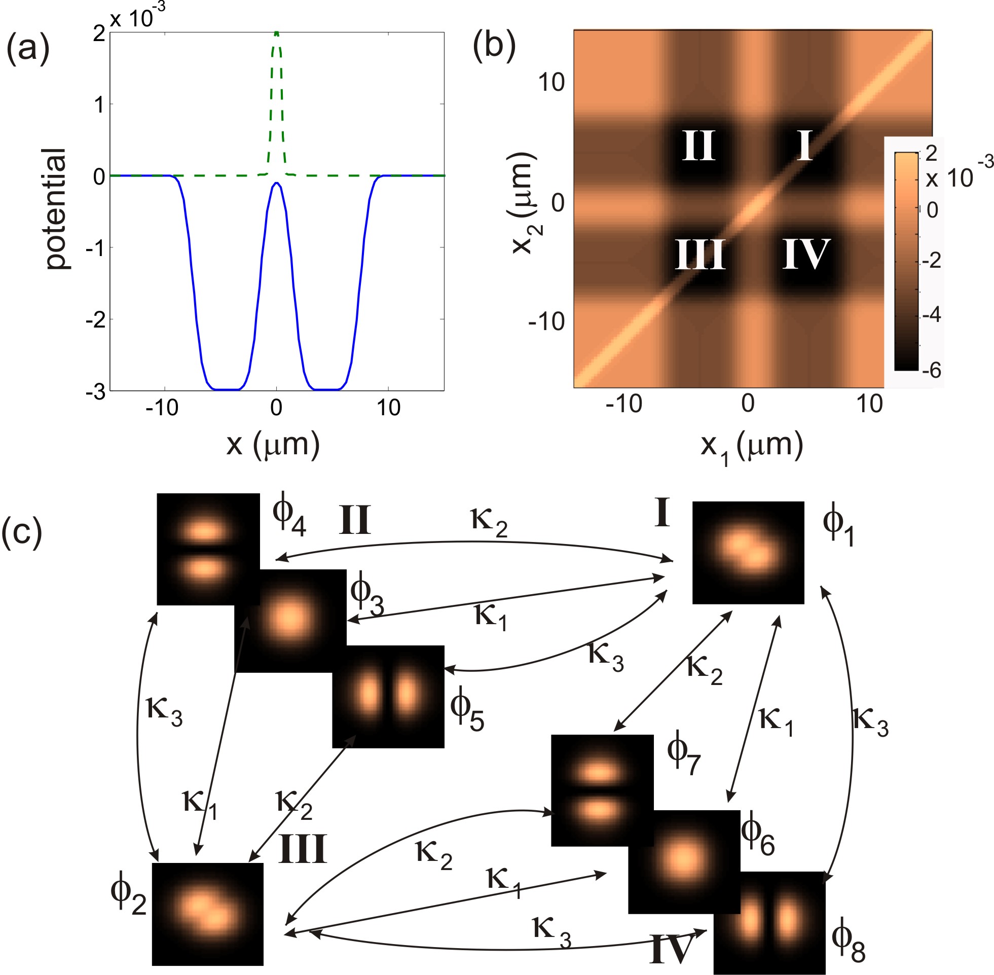
Figure 1: (color online) (a) Profiles of the double well potential $V_{w}(x)$ (solid curve) and of the repulsive potential $V_{int}(x)$ (dashed curve) for parameter values $a=4.5\;\mu$m, $w=3\;\mu$m, $D_{x}=1\;\mu$m, $w_{i}=0.5\;\mu$m, $D_{xi}=0.2\;\mu$m, $\Delta n_{1}=0.003$, and $\Delta n_{2}=0.002$. The corresponding two-dimensional optical potential $V(x_{1},x_{2})$ is shown in (b). (c) Schematic of the guided modes supported by the four core regions involved in the tunneling dynamics and their couplings.

where $\lambdabar=\lambda/(2\pi)$ is the reduced wavelength of photons, $V(x_{1},x_{2})\simeq n_{s}-n(x_{1},x_{2})$ is the optical potential, and $n_{s}$ is the substrate refractive index. The normalization condition $\int_{-\infty}^{\infty}dx_{1}dx_{2}|\psi|^{2}=1$ will be assumed in the following. Previous quantum-optical analogies have generally viewed the paraxial wave equation (1) as formally equivalent to the Schrödinger equation for a single particle of mass $n_{s}$ in a two-dimensional potential $V(x_{1},x_{2})$, in which the temporal evolution of the quantum particle is mapped into the spatial light evolution along the axial direction $z$ and the Planck’s constant is replaced by the reduced wavelength of photons (see, for instance, Longhi05 ). However, whenever the potential $V$ has the form

$$V(x_{1},x_{2})=V_{w}(x_{1})+V_{w}(x_{2})+V_{int}(|x_{1}-x_{2}|),$$ (2)

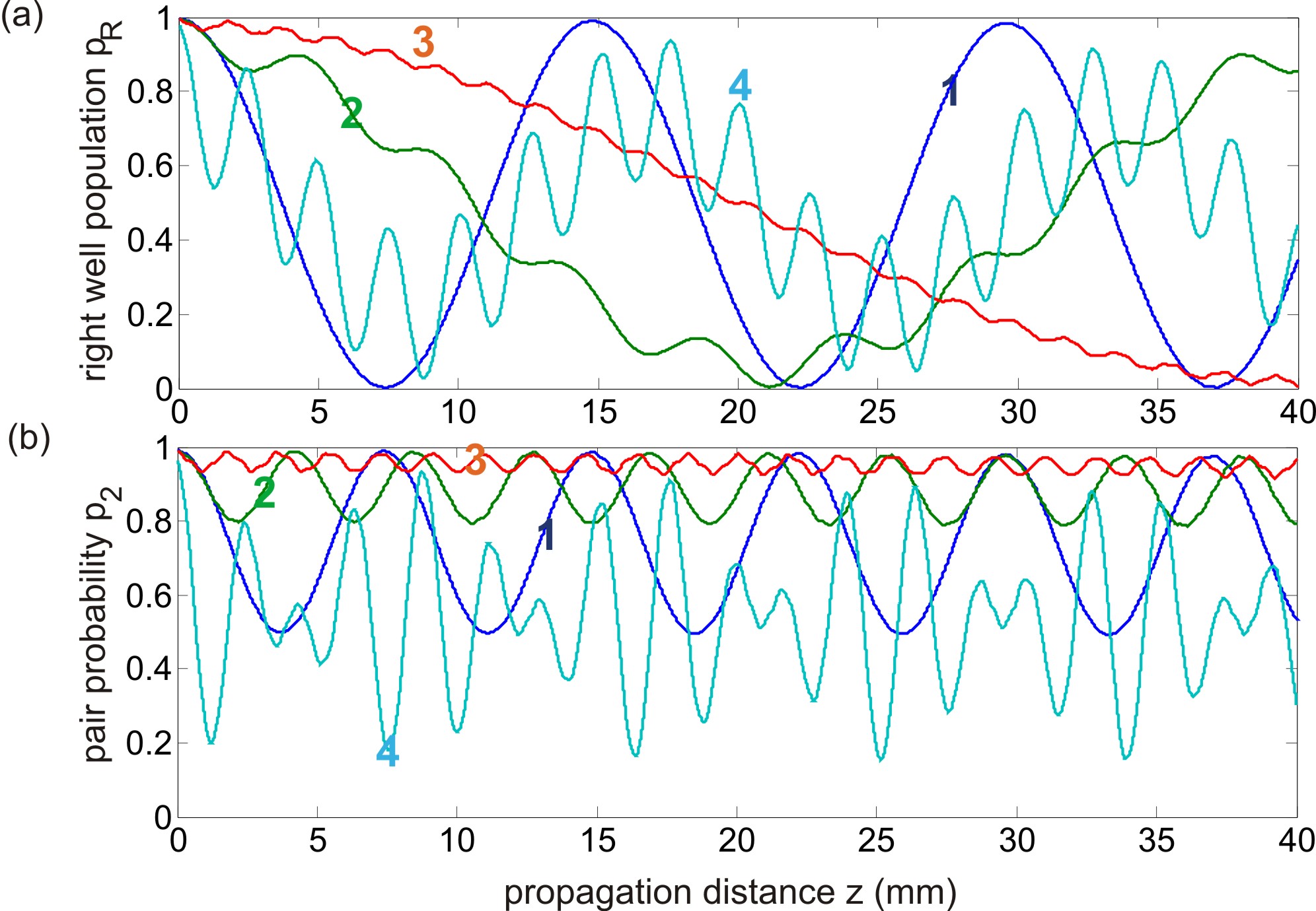
Figure 2: (color online) Numerically-computed behavior of (a) the percentage of bosons in the right well $p_{R}$, and (b) of the pair probability $p_{2}$ versus propagation distance, for increasing values of the particle interaction strength, measured by the index change $\Delta n_{2}$. Curve 1: $\Delta n_{2}=0$ (non-interacting bosons); curve 2: $\Delta n_{2}=0.5\times 10^{-3}$; curve 3: $\Delta n_{2}=1.5\times 10^{-3}$; curve 4: $\Delta n_{2}=15\times 10^{-3}$. Curves 2 and 3 correspond to the correlated pair tunneling regime, whereas curve 4 corresponds to tunneling of a fragmented pair.

where $V_{w}(x)$ is an arbitrary one-dimensional potential and $V_{int}(x)$ is a short-range potential, Eq.(1) can be regarded as the optical analogue of the Schrödinger equation for two particles with the same mass $n_{s}$ in a one-dimensional potential $V_{w}$, which interacts via the potential $V_{int}$. If the optical structure is excited at the $z=0$ input plane by a beam satisfying the symmetry constraint $\psi(x_{1},x_{2},0)=\psi(x_{2},x_{1},0)$, the wave function $\psi$ remains symmetric along the propagation, and Eq.(1) thus describes the evolution of two interacting identical bosons. Therefore, if we assume for $V_{w}$ a double well shape and for $V_{int}$ a short-range repulsive potential, our optical system realizes a classic wave optics analogue of the two-boson junction recently studied in Ref.C4 . In our optical system, we assume for $V_{w}(x)$ a double well of the form DellaValle07 $V_{w}=-\Delta n_{1}[g(x-a)+g(x+a)]$, where $g(x)=[{\rm erf}((x+w)/D_{x})-{\rm erf}((x-w)/D_{x})]/[2{\rm erf}(w/D_{x})]$ is the well shape, $2a$ is the distance between the two wells, $\Delta n_{1}>0$ is the peak index change that defines the well depth, and $2w$ is the well width. For the repulsive potential, we assume a similar functional form $V_{int}=\Delta n_{2}[{\rm erf}((x+w_{i})/D_{xi})-{\rm erf}((x-w_{i})/D_{xi})]/[2{\rm erf}(w_{i}/D_{xi})]$, with $w_{i}$ and $D_{xi}$ much smaller than $w$ and $D_{x}$, respectively. The refractive index change $\Delta n_{2}>0$ measures the strength of the interaction, $\Delta n_{2}=0$ corresponding to non-interacting bosons. Typical shapes of $V_{w}(x)$, $V_{int}(x)$ and of the resulting two-dimensional potential $V(x_{1},x_{2})$ [Eq.(2)] are shown in Figs.1(a) and (b). Note that the resulting potential $V$ in the $(x_{1},x_{2})$ plane defines four higher-index guiding regions, i.e. four waveguides, denoted by I-IV in Fig.1(b), which are evanescently coupled. Such a four-core guide could be realized, for example, with the technology of microstructured fibers fibers , in which a preform with the desired geometrical and refractive index features is first manufactured. For example, using a cladding region made of fused silica, the structure of Fig.1(b) could be realized by assembling different regions of fused silica with different GeO₂ doping concentrations.

III Tunneling dynamics

The main features of the tunneling dynamics of two bosons in a double-well potential are captured by analyzing the evolution of the percentage of bosons in the right well $p_{R}(z)$ and the the pair (or same-site) boson probability $p_{2}(z)$, which are defined by C4

$$p_{R}(z) = \int_{0}^{\infty}dx_{1}\int_{-\infty}^{\infty}dx_{2}|\psi|^{2}$$ (3)

$$p_{2}(z) = \int_{x_{1},x_{2}>0}dx_{1}dx_{2}|\psi|^{2}+\int_{x_{1},x_{2}<0}dx_{1}dx_{2}|\psi|^{2}\;\;\;\;\;\;\;.$$ (4)

In our optical setting, $p_{R}(z)$ and $p_{2}(z)$ simply correspond to the fractional light power trapped in waveguides I and IV, and in waveguides I and III, respectively. A typical evolution of $p_{R}(z)$ and $p_{2}(z)$, as obtained by numerical integration of Eq.(1) for increasing values of the interaction strength $\Delta n_{2}$, is shown in Fig.2. Parameter values used in simulations are $\lambda=633$ nm and $n_{s}=1.45$. In each simulation, the structure is excited at $z=0$ in the fundamental mode of the guide I, which corresponds to have initially the two bosons in the right-side well in the lowest energy state. The scenario shown in Fig.2 reproduces the transition from uncorrelated tunneling to pair tunneling and fragmented tunneling in the fermionization limit, predicted in Ref.C4 . For non-interacting bosons (curve 1), the atoms simply Rabi oscillate back and forth between both wells, and they tunnel independently. As a small correlation is introduced (curve 2), both atoms tend to remain in the same well in the course of tunneling, i.e they tunnel as pairs. Such a dynamical behavior, which was observed in C5 and referred to as second-order tunneling, can be simply explained in the framework of a standard two-site Bose-Hubbard model, the optical simulation of which was recently proposed in the Fock space using waveguide arrays Longhiun . However, the standard Bose-Hubbard model fails to predict the tunneling regimes at strong interaction and the transition to the fermionization limit. Indeed, at a larger interaction (curve 3), tunneling tends to be inhibited, which is the few-body signature of the self-trapping phenomenon of many bosons in the mean-field limit. Remarkably, at stronger interaction and near the fermionization limit (curve 4), tunneling is again allowed, and a fast oscillation of $p_{R}(z)$ is superimposed to the slower tunneling cycle. This basically corresponds to fragmented-pair tunneling at the Rabi frequency predicted in Ref.C4 . Correspondingly, $p_{2}(z)$ passes through just about any value from 1 (fragmented pair) to small values (near complete isolation). A detailed explanation of such a rich tunneling scenario requires an inspection of the low-lying energy spectrum of the exact two-boson Hamiltonian (1) beyond the standard two-mode Bose-Hubbard approximation C4 . In the optical context, the scenario can be explained in a different view as the result of evanescent photonic tunneling among a few guided modes of the four two-dimensional guides in the geometrical setting of Fig.1(b). In fact, let us indicate by $\phi_{1,2}$ the fundamental modes of the isolated waveguides I and III, by $\phi_{3,4,5}$ the fundamental and the two lowest higher-order degenerate transverse modes of the isolated waveguide II, and by $\phi_{6,7,8}$ the fundamental and the two lowest higher-order degenerate transverse modes of the isolated waveguide IV. A typical profile of such modes is shown in Fig.1(c). Let then expand the envelope $\psi$ as a superposition of such modes with $z$-varying coefficients, i.e. $\psi=\sum_{l=1}^{8}c_{l}(z)\phi_{l}(x_{1},x_{2})\exp(i\beta z)$, where $\beta$ is a reference propagation constant. Note that, for symmetry reasons, one has $c_{6}=c_{3}$, $c_{7}=c_{4}$ and $c_{8}=c_{5}$. In the tight-binding and nearest-neighboring approximation, neglecting cross-coupling terms, the following coupled-mode equations for the amplitudes $c_{l}$ can be derived (see, for instance, Christodoulides03 ; Ruffo ):

$$i(dc_{1}/dz) = -2\kappa_{1}c_{3}-2\kappa_{2}c_{4}-2\kappa_{3}c_{5}+\delta_{1}c_{1}$$

$$i(dc_{2}/dz) = -2\kappa_{1}c_{3}-2\kappa_{3}c_{4}-2\kappa_{2}c_{5}+\delta_{1}c_{2}$$

$$i(dc_{3}/dz) = -\kappa_{1}(c_{1}+c_{2})$$ (5)

$$i(dc_{4}/dz) = -\kappa_{2}c_{1}-\kappa_{3}c_{2}+\delta_{2}c_{4}$$

$$i(dc_{5}/dz) = -\kappa_{3}c_{1}-\kappa_{2}c_{2}+\delta_{2}c_{5}$$

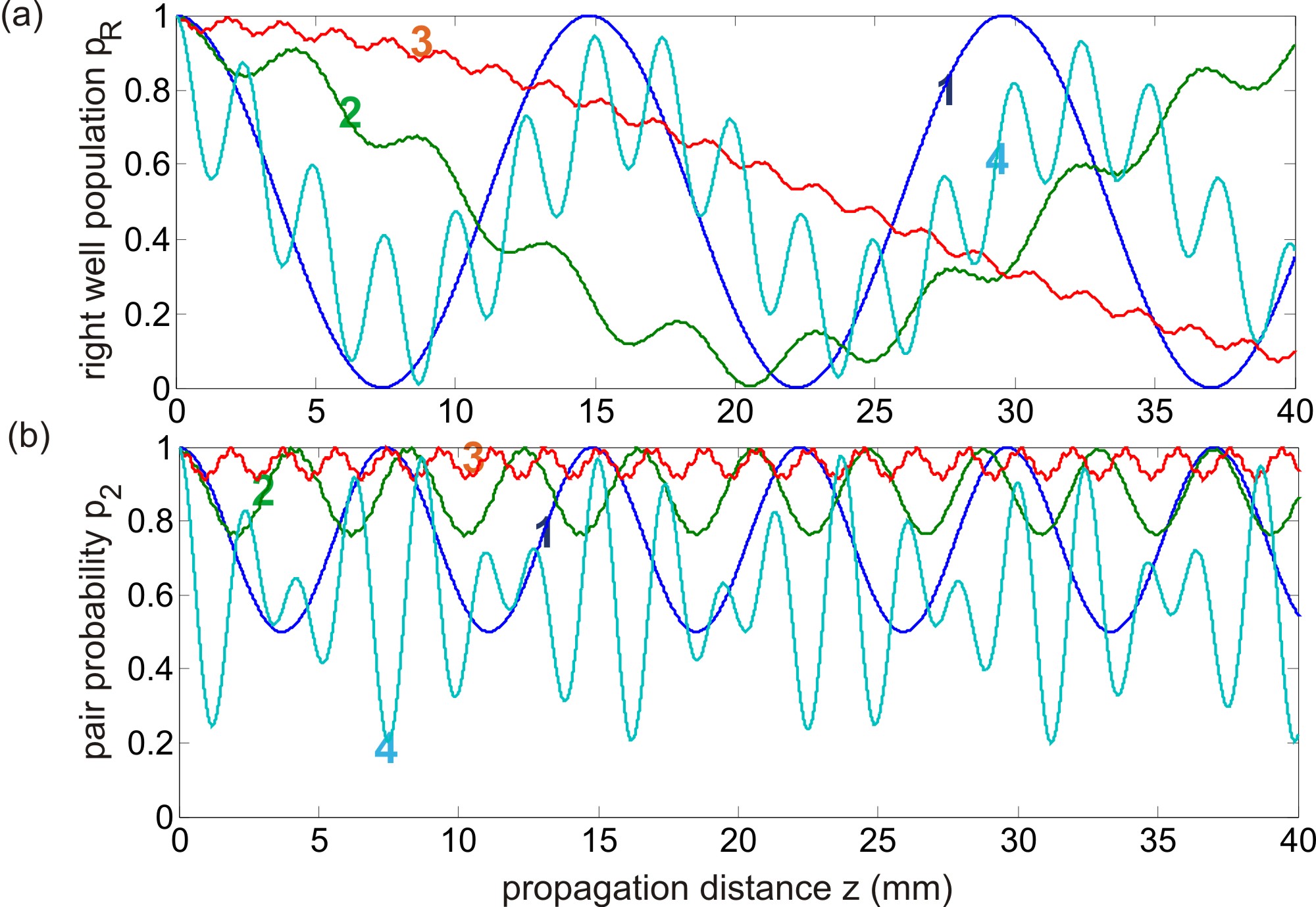
Figure 3: (color online) (a) Behavior of $p_{R}$, and (b) of $p_{2}$ versus propagation distance, for increasing values of particle interaction strength measured by the detuning $\delta_{1}$, as predicted by the coupled-mode equations (3), for $\kappa_{2}=0.16$, $\kappa_{3}=0.80$, and $\delta_{2}=20$ (in units of ${\rm mm}^{-1}$). Curve 1: $\delta_{1}=0$, $\kappa_{1}=0.212$; curve 2: $\delta_{1}=1.22$, $\kappa_{1}=0.26$; curve 3: $\delta_{1}=3.2$, $\kappa_{1}=0.32$; curve 4: $\delta_{1}=18.9$, $\kappa_{1}=0.38$.

where $\kappa_{1}$, $\kappa_{2}$ and $\kappa_{3}$ are the coupling constants between the couples of modes $\{\phi_{1},\phi_{3}\}$, $\{\phi_{1},\phi_{4}\}$ and $\{\phi_{1},\phi_{5}\}$, respectively [see Fig.1(c)], $\delta_{1}=\beta_{3}-\beta_{1}$ is the mismatch between the propagation constants $\beta_{3}$ and $\beta_{1}$ of modes $\phi_{3}$ and $\phi_{1}$, and $\delta_{2}=\beta_{3}-\beta_{4}$ is the mismatch between the propagation constants $\beta_{3}$ and $\beta_{4}$ of modes $\phi_{3}$ and $\phi_{4}$ (or $\phi_{5}$). Initial condition for Eqs.(5) is $c_{l}(0)=\delta_{l,1}$. In terms of the amplitudes $c_{l}$, the percentage of bosons in the right well and the same-site boson probability, as defined by Eqs.(3) and (4), take take the simple form

$$p_{R}(z) = |c_{1}|^{2}+|c_{3}|^{2}+|c_{4}|^{2}+|c_{5}|^{2}$$ (6)

$$p_{2}(z) = |c_{1}|^{2}+|c_{2}|^{2},$$ (7)

respectively. In the absence of interaction, i.e. for $\Delta n_{2}=0$, one has $\delta_{1}=0$ whereas $\delta_{2}$ is much larger than the coupling constants. Hence, the higher-order transverse modes of waveguides II and IV are not excited, i.e. one has $c_{4}\sim c_{5}\sim 0$, and the evolution of $c_{1}$, $c_{2}$ and $c_{3}$ can be calculated exactly, yielding $p_{R}(z)=\cos^{2}(\kappa_{1}z)$ and $p_{2}(z)=(1/2)[1+\cos^{2}(2\kappa_{1}z)]$: this is precisely the dynamical behavior of uncorrelated bosons (curve 1 of Fig.2). As the interaction $\Delta n_{2}$ is increased, the detuning $\delta_{1}$ increases, whereas $\delta_{2}$ does not change. The coupling constants $\kappa_{1}$, $\kappa_{2}$ and $\kappa_{3}$ are given by overlapping integrals involving the coupled guided modes, and are expected to slightly increase as $\Delta n_{2}$ is increased because of the less confinement of modes $\phi_{1}$ and $\phi_{2}$. If $(\delta_{2}-\delta_{1})$ is still large enough that the higher-order transverse modes of waveguides II and IV are still out of resonance, the amplitudes $c_{4}$ and $c_{5}$ remain small, and the tunneling dynamics is mainly governed by the first three equations of the system (3), but with $\delta_{1}\neq 0$. A nonvanishing value of the detuning $\delta_{1}$ is responsible for the doubly-periodicity of $p_{R}(z)$, the increase of the tunneling period, and the appearance of correlated pair tunneling (i.e. $p_{2}(z)\simeq 1$) as observed in curves 2 and 3 of Fig.2. As the interaction $\Delta n_{2}$ is further increased, excitation of the higher-order transverse modes of waveguides II and IV can not be anymore neglected, and the tunneling dynamics requires to account for the full five amplitudes entering in Eq.(5). For very strong interactions, corresponding to the fermionization limit, the fundamental modes $\phi_{1,2}$ of waveguides I and III get close to resonance with the (degenerate) transverse modes $\phi_{4,5}$ and $\phi_{7,8}$ of waveguides II and IV, whereas their fundamental modes $\phi_{3,6}$ are now out of resonance. Hence, in the fermionization limit one can set $c_{3}\simeq 0$ in Eqs.(5). Such equations well describe the restoration of tunneling of a fragmented pair.

A typical dynamical evolution of $p_{R}(z)$ and $p_{2}(z)$ in the various parameter regions, as obtained by numerically solving the coupled-mode equations (5) by varying $\delta_{1}$ and taking into account for the correction of $\kappa_{1}$ solely, is shown in Fig.3.

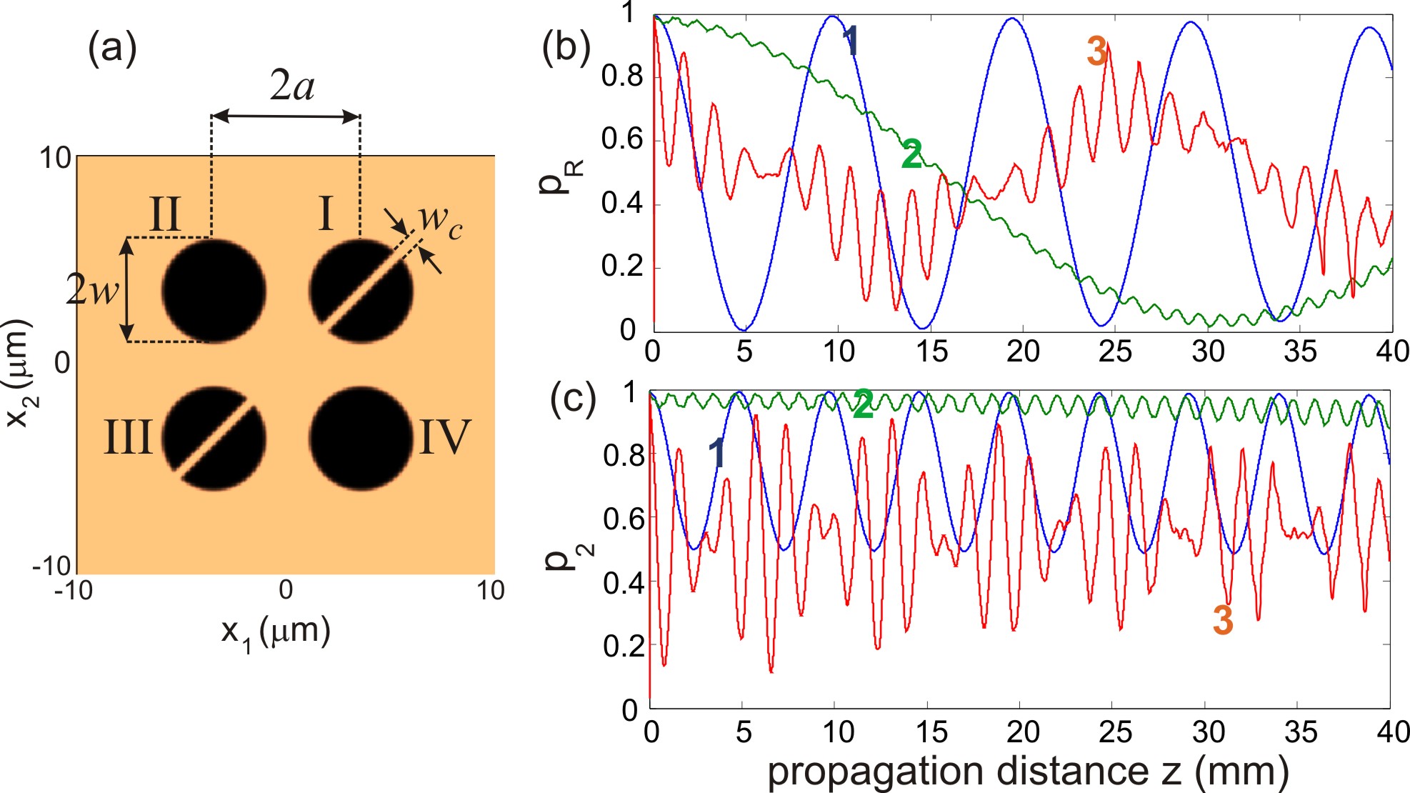
Figure 4: (color online) Light tunneling dynamics in a four-core fiber. (a) Profile of the optical potential $n_{s}-n(x_{1},x_{2})$ (core diameter $2w=5\;\mu$m, core spacing $2a=7\;\mu$m, index change $\Delta n=0.005$). (b) and (c) show the evolution of $p_{R}$ and $p_{2}$, respectively, for increasing values of the width $w_{c}$ of the cut in guides I and III. Curve 1: $w_{c}=0$ (non-interacting bosons); curve 2: $w_{c}=0.6\;\mu$m (correlated pair tunneling); curve 3: $w_{c}=2\;\mu$m (tunneling of a fragmented pair).

Note that the behavior of both the percentage of bosons in the right well and the same-site boson probability reproduces very well the different tunneling regimes previously found in Fig.2.

The good description of the tunneling dynamics offered by the coupled-mode equations (5) indicates that the tunneling dynamics of two bosons, shown in Fig.2, is rather insensitive to the specific shapes of the guides, and could be thus observed in simpler optical structures. For example, in Fig.4 it is shown that a similar dynamical behavior can be realized using a microstructured optical fiber with four circular cores of radius $w$ and step-index $\Delta n$, in which a cut with variable width $w_{c}$ is applied to the cores I and III to mimic boson repulsion [Fig.4(a)]. As the cut width $w_{c}$ (i.e. the interaction strength) is increased, a transition from independent Rabi oscillations (curve 1) to correlated pair tunneling (curve 2) and to tunneling of a fragmented pair (curve 3) ic clearly observed.

IV Conclusions

In conclusion, an optical realization of the tunneling dynamics of two interacting bosons in a double-well potential, based on light transport in a four-core microstructured fiber, has been proposed. The present results indicate that photonic systems could provide an experimentally accessible test bench to investigate in a purely classical setting the dynamical aspects embodied in the physics of strongly-correlated few-particle quantum systems. As compared to quantum simulators based on the coherent dynamics of cold atoms or ions trapped in optical lattices JPBreview , the use of a classical optics simulator enables a direct access to the evolution of the multiparticle probability density and could provide a new route to realize other many-body physical models Longhiun ; Korsch . For example, the introduction of gain and loss regions in the optical structure could offer the possibility to test in the lab the physics of many-body particles within non-Hermitian $\mathcal{PT}$-symmetric models Korsch .

- (1) D.N. Christodoulides, F. Lederer, and Y. Silberberg, Nature (London) 424, 817 (2003).
- (2) S. Longhi, Laser and Photon. Rev. 3, 243 (2009).
- (3) H. Trompeter, T. Pertsch, F. Lederer, D. Michaelis, U. Streppel, A. Bräuer, and U. Peschel, Phys. Rev. Lett. 96, 023901 (2006).
- (4) S. Longhi, M. Marangoni, M. Lobino, R. Ramponi, P. Laporta, E. Cianci, and V. Foglietti, Phys. Rev. Lett. 96, 243901 (2006); A. Szameit, I.L. Garanovich, M. Heinrich, A.A. Sukhorukov, F. Dreisow, T. Pertsch, S. Nolte, A. Tünnermann, and Y.S. Kivshar, Nat. Phys. 5, 271 (2009).
- (5) T. Schwartz, G. Bartal, S. Fishman, and M. Segev, Nature (London) 446, 52 (2007); Y. Lahini, A. Avidan, F. Pozzi, M. Sorel, R. Morandotti, D. N. Christodoulides, and Y. Silberberg, Phys. Rev. Lett. 100, 013906 (2008).
- (6) G. Della Valle, M. Ornigotti, E. Cianci, V. Foglietti, P. Laporta, and S. Longhi, Phys. Rev. Lett. 98, 263601 (2007).
- (7) P. Biagioni, G. Della Valle, M. Ornigotti, M. Finazzi, L. Duó, P. Laporta, and S. Longhi, Opt. Express 16, 3762 (2008); F. Dreisow, A. Szameit, M. Heinrich, T. Pertsch, S. Nolte, A. Tünnermann, and S. Longhi, Phys. Rev. Lett. 101, 143602 (2008).
- (8) S. Longhi, M. Marangoni, D. Janner, R. Ramponi, P. Laporta, E. Cianci, and V. Foglietti, Phys. Rev. Lett. 94, 073002 (2005).
- (9) X. Zhang, Phys. Rev. Lett. 100, 113903 (2008); F. Dreisow, M. Heinrich, R. Keil, A. Tünnermann, S. Nolte, S. Longhi, and A. Szameit, Phys. Rev. Lett. 105, 143902 (2010).
- (10) J.J. García-Ripoll, P. Zoller, and J.I. Cirac, J. Phys. B 38, S567 (2005); M. Johanning, A.F. Varon and C. Wunderlich, J. Phys. B 42, 154009 (2009).
- (11) R. Gati and M.K. Oberthaler, J. Phys. B 40, R61 (2007).
- (12) M. Albiez, R. Gati, J. Fölling, S. Hunsmann, M. Cristiani, and M.K. Oberthaler, Phys. Rev. Lett. 95, 010402 (2005).
- (13) S. Levy, E. Lahoud, I. Shomroni, and J. Steinhauer, Nature (London) 449, 579 (2007).
- (14) S. Fölling, S. Trotzky, P. Cheinet, M. Feld, R. Saers, A. Widera, T.Müller, and I. Bloch, Nature (London) 448, 1029 (2007).
- (15) S. Zöllner, H.-D. Meyer, and P. Schmelcher, Phys. Rev. Lett. 100, 040401 (2008); S. Zöllner, H.-D. Meyer, and P. Schmelcher, Phys. Rev. A 78, 013621 (2008).
- (16) K. Sakmann, A.I. Streltsov, O.E. Alon, and L.S. Cederbaum, Phys. Rev. Lett. 103, 220601 (2009).
- (17) J. Gong, L. Morales-Molina, and P. Hänggi, Phys. Rev. Lett. 103, 133002 (2009).
- (18) S.M. Jensen, IEEE J. Quantum Electron. 18, 1580, (1982); R. Khomeriki, J. Leon, and S. Ruffo, Phys. Rev. Lett. 97, 143902 (2006).
- (19) S. Zöllner, H.-D. Meyer, and P. Schmelcher, Phys. Rev. A 74, 053612 (2006); J.-Q. Liang, J.-L. Liu, W.-D. Li, and Z.-J. Li, Phys. Rev. A 79, 033617 (2009); B. Chatterjee, I. Brouzos, S. Zöllner, and P. Schmelcher, Phys. Rev. A 82, 043619 (2010).
- (20) O.E. Alon and L.S. Cederbaum, Phys. Rev. Lett. 95, 140402 (2005).
- (21) K. Winkler, G. Thalhammer, F. Lang, R. Grimm, J. Hecker Denschlag, A.J. Daley, A. Kantian, H. P. Büchler, and P. Zoller, Nature (London) 441, 853 (2006).
- (22) M. Bayindir, A. F. Abouraddy, O. Shapira, J. Viens, D. Saygin-Hinczewski, F. Sorin, J. Arnold, J. D. Joannopoulos, and Y. Fink, IEEE J. Sel. Top. Quantum Electron. 12, 1202 (2006).
- (23) S. Longhi, J. Phys. B 44, 051001 (2011); S. Longhi Phys. Rev. A 83, 034102 (2011).
- (24) E.M. Graefe, H.J. Korsch, and A. E. Niederle, Phys. Rev. Lett. 101, 150408 (2008).