Gelfond-Bézier Curves

Abstract

We show that the generalized Bernstein bases in Müntz spaces defined by Hirschman and Widder [7] and extended by Gelfond [6] can be obtained as limits of the Chebyshev-Bernstein bases in Müntz spaces with respect to an interval $[a,1]$ as $a$ converges to zero. Such a realization allows for concepts of curve design such as de Casteljau algorithm, blossom, dimension elevation to be translated from the general theory of Chebyshev blossom in Müntz spaces to these generalized Bernstein bases that we termed here as Gelfond-Bernstein bases. The advantage of working with Gelfond-Bernstein bases lies in the simplicity of the obtained concepts and algorithms as compared to their Chebyshev-Bernstein bases counterparts.

1 Introduction

This work was motivated by the following rather surprising observation : Let $r_{1},...,r_{n}$ be $n$ real numbers such that $0<r_{1}<r_{2}<...<r_{n}$. Then, for any interval $[a,b]$ such that $0<a<b$, the linear Müntz space

$$E=span(1,t^{r_{1}},t^{r_{2}},...,t^{r_{n}})$$ (1)

possesses a particular basis $(B_{0},B_{1},...,B_{n})$ called the Chebyshev-Bernstein basis with respect to the interval $[a,b]$ and can be characterized by the following two properties [11]: For any $t\in[a,b]$, we have

$$\sum_{k=0}^{n}B_{k}(t)=1$$ (2)

and for any $k=0,...,n$, the function $B_{k}$ has a zero of order $k$ at $a$ and a zero of order $(n-k)$ at $b$. The Müntz space $E$ also possesses a different basis, called generalized Bernstein basis, that were first defined by Hirschman and Widder [7], extended by Gelfond [6] and popularized in Lorentz’s book [8]. Due to the fact that there is a variety of bases in the literature that are also termed generalized Bernstein polynomials or bases [5, 15] and because the account given in Lorentz’s book for these generalized Bernstein bases follows more the approach taken by Gelfond than the one taken by Hirschman and Widder, we call these bases here, the Gelfond-Bernstein bases. The Gelfond-Bernstein bases are in some sense a generalization of the classical Bernstein base over the interval $[0,1]$ of the linear space of polynomials. The Chebyshev-Bernstein bases are defined only with respect to intervals $[a,b]$ such that $a>0$. Our observation is the fact that when $b=1$ and $a$ converges to zero, the Chebyshev-Bernstein bases over the interval $[a,b]$ coincide with the Gelfond-Bernstein bases. To understand the peculiarity and then the consequences of this result, we should first recall the historical reasons for defining the Gelfond-Bernstein bases. In 1912, Bernstein found an ingenious method of proving the Weierstrass approximation Theorem, by defining what we now know as the Bernstein basis of the linear space of polynomials [3]. In 1914, Müntz , answering a conjecture of Bernstein, generalized the Weierstrass Theorem in the following sense [12]: Given a sequence of positive real numbers $r_{1}<r_{2}<...<r_{n}<..$ such that $\lim_{n\to\infty}r_{n}=\infty$, then the linear space $E=span(1,t^{r_{1}},t^{r_{2}},...,t^{r_{n}},...)$ is a dense subset of the space $C\left([0,1]\right)$ of continuous functions over the interval $[0,1]$ endowed with the uniform norm if and only if

$$\sum_{i=1}^{\infty}\frac{1}{r_{i}}=\infty.$$ (3)

The proof given by Müntz of the if part of the Theorem involved rather complicated techniques on summation of Fourier series. It was then an interesting and rather difficult problem of whether there exists a suitable generalization of Bernstein polynomials that could lead to a new proof of the if part of Müntz Theorem in a fashion similar to Bernstein proof of the Weierstrass Theorem. Such generalized Bernstein bases were found by Hirschman and Widder in 1949. Their proof of the if part of Müntz theorem was modified and generalized by Gelfond in 1958. These generalized Bernstein bases (Gelfond-Bernstein bases) were defined to specifically handle the problem of density of Müntz spaces as a subset of the space of continuous functions over the interval $[0,1]$ (or the interval $[0,b]$, $b>0$ through a change of variable). The only hints that these generalized Bernstein bases were the most suitable one are the fact that they satisfy (2), they are non-negative in the interval $[0,1]$ and most importantly that they achieve the right generalization for proving Müntz Theorem. Now, coming to a more recent history, Pottmann, in 1993, defined the notion of Chebyshev blossom associated with any linear space $F=span\left(1,\phi_{1},\phi_{2},...,\phi_{n}\right)$ such that $span\left(\phi_{1}^{\prime},\phi_{2}^{\prime},...,\phi_{n}^{\prime}\right)$ is an extended Chebyshev space of order $n$ on an interval [13]. Chebyshev blossoming allows for a natural definition of the notion of Chebyshev-Bernstein basis associated with the linear space $F$ and which reveal striking similarities with the classical notions associated with the Bernstein-Bézier framework such as the notions of control points, de Casteljau algorithm, subdivision schemes, dimension elevation. In the case of the Müntz space $E$ in (1), we can define the notion of Chebyshev-Bernstein basis only on interval $[a,b]$ such that $a>0$. Therefore, a way to define a notion of Chebyshev-Bernstein basis of the space $E$ over the interval $[0,1]$ is to hope that taking the limit of Chebyshev-Bernstein basis on the interval $[a,1]$ with $a>0$ as $a$ converges to zero leads to meaningful expressions that constitute a basis of the space $E$. Our observation is that in doing so, we did not only defined the “Chebyshev-Bernstein basis” over the interval $[0,1]$, but we also discover that they coincide with the Gelfond-Bernstein basis. This result reflects, first of all, the ingenuity of Hirschmann, Widder and Gelfond in defining the right generalized Bernstein bases with little knowledge at the time of the most natural criteria for such a generalization. Furthermore, this result legitimates the use of Gelfond-Bernstein bases in computer aided geometric design and in which the CAGD concepts can be translated from the Chebyshev-Bernstein bases to Gelfond-Bernstein bases by a limiting process. As we will exhibit in this work, several useful properties of the Gelfond-Bernstein bases could be simply proven without resort to the limiting process. However, the notion of blossom and the derivation of the de Casteljau algorithm are not obvious from the classical definition of the Gelfond-Bernstein bases and should be derived from the limiting process. Including the point zero in the interval under consideration through the limiting process will have an effect of collapsing difficult expressions in the theory of Chebyshev blossoms in Müntz spaces to highly simpler ones. Such simplifications are achieved through a splitting concept in the theory of Schur functions. This provides the theory of Gelfond-Bernstein bases with simpler algorithms as compared to their Chebyshev-Bernstein bases counterparts. The paper is organized as follows. In section 2, we recall some basic properties of Schur functions. In section 3, we recall our main results in [1] regarding Chebyshev blossoming in Müntz spaces and in which the Chebyshev blossom and the Chebyshev-Bernstein bases are expressed in terms of Schur functions. The definition of the Gelfond-Bernstein bases, as well as the proof that they coincide with the Chebyshev-Bernstein bases through a limiting process will be given in section 4. In section 5, we study the notion of Gelfond-Bézier curves, thereby demonstrating their adequacy to be incorporated into CAGD tools. The expression of Chebyshev-Bernstein bases in Müntz spaces are given in terms of Schur functions, while the definition of Gelfond-Bernstein bases involves divided differences. The connection between the two bases leads to a simple expression of the divided differences in terms of Schur functions. We will exhibit the usefulness of such expression by providing the Gelfond-Bernstein bases of some specific Müntz spaces. In section 7, we define the blossom associated with Gelfond-Bézier curves and give a method of deriving the de Casteljau algorithm in Müntz spaces. In section 8, we study the concept of dimension elevation algorithms of Gelfond-Bézier curves. We define the notion of shifted Gelfond-Bézier curves in section 9, and show their adequacy in curve design. We conclude in Section 10.

2 Schur Functions

The theory of Schur functions will play a fundamental role in this work. Therefore, in this section, we fix notations and review some basic concepts in the theory. In the case of Schur functions associated with integer partitions, we will follow the standard Macdonald’s notations [9].

A sequence $\lambda=(\lambda_{1},\lambda_{2},...,\lambda_{n})$ of real numbers is said to be a real partition if it satisfies

$$\lambda_{1}>\lambda_{2}-1>\lambda_{3}-2>...>\lambda_{n}-(n-1)>-n.$$

The Schur function indexed by a real partition $\lambda$ is defined as

$$S_{\lambda}(u_{1},...,u_{n})=\frac{\det(u_{i}^{\lambda_{j}+n-j})_{{1\leq i,j\leq n}}}{\prod_{1\leq i<j\leq n}(u_{i}-u_{j})},$$ (4)

with the convention that L’Hospital’s rule is applied whenever there are equalities among $u_{1},u_{2},...,u_{n}$. Note that if $\lambda=(\lambda_{1},\lambda_{2},...,\lambda_{n})$ is a real partition, then $(\lambda_{1},\lambda_{2},...,\lambda_{n},0)$ is also a real partition. Therefore, we will adopt the convention that if the number of variables in the Schur function is larger than the number of components in the real partition, then we add zeros to the real partition. For example, we will write $S_{(\lambda_{1},\lambda_{2})}(u_{1},u_{2},u_{3},u_{4})$ to mean $S_{(\lambda_{,}\lambda_{2},0,0)}(u_{1},u_{2},u_{3},u_{4})$. In the case the elements of the sequence $\lambda$ are positive integers, we recover the classical notion of integer partitions and in which the associated Schur function $S_{\lambda}(u_{1},...,u_{n})$ is an element of the ring $\mathbb{Z}[u_{1},...,u_{n}]$. For integer partitions, we will follow the following terminology and conventions. The total number of non-zero components, $l(\lambda)$, will be called the length of the integer partition $\lambda$. We will always ignore the difference between two integer partitions that differ only in the number of their trailing zeros. The non-zero $\lambda_{i}$ of the partition will be called the parts of $\lambda$. The weight $|\lambda|$ of a partition $\lambda$ is defined as the sum its parts i.e., $|\lambda|=\sum_{i=1}^{\infty}\lambda_{i}$. We will find it sometimes convenient to write a partition by the common notation that indicate the number of times each integer appears as a part in the partition, for example we write the partition $\lambda=(4,4,4,3,3,1)$ as $\lambda=(4^{3},3^{2},1)$. We will adopt the convention that $S_{\lambda}(u_{1},...,u_{n})\equiv 0$ if $l(\lambda)>n$. From the definition, the Schur function associated with the empty partition $\lambda=(0,...,0,..)$ is $S_{\lambda}(u_{1},...,u_{n})\equiv 1$. For the partition $\lambda=(r)$, the Schur function $S_{\lambda}$ is the complete symmetric function $h_{r}$ i.e.,

$$S_{(r)}(u_{1},u_{2},...,u_{n})=h_{r}(u_{1},...,u_{n})=\sum_{i_{1}\leq i_{2}\leq...\leq i_{r}}u_{i_{1}}u_{i_{2}}...u_{i_{r}},$$

while for the partition $\lambda=(1^{r})$ with $r\leq n$, the Schur function $S_{(1^{r})}$ is given by the elementary symmetric function $e_{r}$ i.e,

$$S_{(1^{r})}(u_{1},u_{2},...,u_{n})=e_{r}(u_{1},...,u_{n})=\sum_{i_{1}<i_{2}<...<i_{r}}u_{i_{1}}u_{i_{2}}...u_{i_{r}}.$$

The Schur function $S_{\lambda}$, with $\lambda$ an integer partition, can be expressed in terms of the complete symmetric functions through the Jacobi-Trudi formula

$$S_{\lambda}=\det\left(h_{\lambda_{i}-i+j}\right)_{1\leq i,j\leq n},$$ (5)

where we assume that $h_{m}\equiv 0$ if $m<0$. The conjugate, $\lambda^{\prime}$, of an integer partition $\lambda$ is the integer partition whose Young diagram is the transpose of the Young diagram of $\lambda$, equivalently $\lambda^{\prime}_{i}=Card\{j|\lambda_{j}\geq i\}.$ Using the conjugate partition, Schur functions can be expressed in terms of the elementary symmetric functions through the Nägelsbach-Kostka formula

$$S_{\lambda}=\det\left(e_{\lambda_{i}^{\prime}-i+j}\right)_{1\leq i,j\leq n},$$

where we assume that $e_{m}\equiv 0$ if $m<0$. Throughout this work, we will use the notation

$$S_{\lambda}(u_{1}^{m_{1}},u_{2}^{m_{2}},...,u_{k}^{m_{k}}),$$

to mean the evaluation of the Schur function in which the argument $u_{1}$ is repeated $m_{1}$ times, the argument $u_{2}$ is repeated $m_{2}$ times and so on. Combinatorial definition of Schur functions: The Young diagram of an integer partition $\lambda$ is a sequence of $l(\lambda)$ left-justified row of boxes, with the number of boxes in the $i$th row being $\lambda_{i}$ for each $i$. A box $x=(i,j)$ in the diagram of $\lambda$ is the box in row $i$ from the top and column $j$ from the left. For example the Young diagram of the partition $\lambda=(5,4,2)$ and the coordinate of its boxes are

$$\lambda=(5,4,2)\qquad{\vbox{\vbox{\offinterlineskip \moveright 0.0pt\vbox{ \hrule height=0.3pt\hbox{\vrule height=15.52005pt,width=0.3pt,depth=3.87993pt\hbox to19.4pt{\hfil$\mbox{\small{(1,1)}}$\hfil}\vrule height=15.52005pt,width=0.3pt,depth=3.87993pt\hbox to19.4pt{\hfil$\mbox{\small{(1,2)}}$\hfil}\vrule height=15.52005pt,width=0.3pt,depth=3.87993pt\hbox to19.4pt{\hfil$\mbox{\small{(1,3)}}$\hfil}\vrule height=15.52005pt,width=0.3pt,depth=3.87993pt\hbox to19.4pt{\hfil$\mbox{\small{(1,4)}}$\hfil}\vrule height=15.52005pt,width=0.3pt,depth=3.87993pt\hbox to19.4pt{\hfil$\mbox{\small{(1,5)}}$\hfil}\vrule height=15.52005pt,width=0.3pt,depth=3.87993pt}\hrule height=0.3pt}\vspace{-\y@linethick} \moveright 0.0pt\vbox{ \hrule height=0.3pt\hbox{\vrule height=15.52005pt,width=0.3pt,depth=3.87993pt\hbox to19.4pt{\hfil$\mbox{\small{(2,1)}}$\hfil}\vrule height=15.52005pt,width=0.3pt,depth=3.87993pt\hbox to19.4pt{\hfil$\mbox{\small{(2,2)}}$\hfil}\vrule height=15.52005pt,width=0.3pt,depth=3.87993pt\hbox to19.4pt{\hfil$\mbox{\small{(2,3)}}$\hfil}\vrule height=15.52005pt,width=0.3pt,depth=3.87993pt\hbox to19.4pt{\hfil$\mbox{\small{(2,4)}}$\hfil}\vrule height=15.52005pt,width=0.3pt,depth=3.87993pt}\hrule height=0.3pt}\vspace{-\y@linethick} \moveright 0.0pt\vbox{ \hrule height=0.3pt\hbox{\vrule height=15.52005pt,width=0.3pt,depth=3.87993pt\hbox to19.4pt{\hfil$\mbox{\small{(3,1)}}$\hfil}\vrule height=15.52005pt,width=0.3pt,depth=3.87993pt\hbox to19.4pt{\hfil$\mbox{\small{(3,2)}}$\hfil}\vrule height=15.52005pt,width=0.3pt,depth=3.87993pt}\hrule height=0.3pt}\vspace{-\y@linethick} }}}$$

A semi-standard tableau $T^{\lambda}$ with entries less or equal to $n$ is a filling-in the boxes of the integer partition $\lambda$ with numbers from $\{1,2,...,n\}$ making the rows increasing when read from left to right and the column strictly increasing when read from the top to bottom. We say that the shape of $T^{\lambda}$ is $\lambda$. For each semi-standard tableau $T^{\lambda}$ of the shape $\lambda$, we denote by $p_{i}$ the number of occurrence of the number $i$ in the semi-standard tableau $T^{\lambda}$. The weight of $T^{\lambda}$ is then defined as the monomial

$$u^{T^{\lambda}}=u_{1}^{p_{1}}u_{2}^{p_{2}}...u_{n}^{p_{n}}.$$

For a given integer partition $\lambda$ of length at most $n$, the Schur function $S_{\lambda}(u_{1},...,u_{n})$ is given by

$$S_{\lambda}(u_{1},u_{2},...,u_{n})=\sum_{T^{\lambda}}u^{T^{\lambda}},$$

where the sum run over all the semi-standard tableaux of shape $\lambda$ and entries at most $n$.

Example 1.

Consider the partition $\lambda=(2,1)$ and $n=3$. Then, the Young diagram of $\lambda$ and the complete list of semi-standard tableaux of shape $\lambda$ are

   $$1 1 2 1 1 3 1 2 3 1 3 2 1 2 2 1 3 3 2 2 3 2 3 3$$                                                                                                                                                 

Therefore, the Schur function associated with the partition $\lambda$ is given by

$$S_{\lambda}(u_{1},u_{2},u_{3})=u_{1}^{2}u_{2}+u_{1}^{2}u_{3}+2u_{1}u_{2}u_{3}+u_{2}^{2}u_{3}+u_{2}u_{3}^{2}+u_{1}u_{2}^{2}+u_{1}u_{3}^{2}.$$

Giambelli formula: The Young diagram of an integer partition $\lambda$ is said to be a hook diagram if the partition $\lambda$ is of the shape $\lambda=(p+1,1^{q})$ i.e.,

$q\left\{{\hbox{}\vbox{\vbox{\offinterlineskip\vbox{\hrule height=0.3pt\hbox{\vrule height=8.74669pt,width=0.3pt,depth=2.18663pt\hbox to10.93333pt{\hfil}\vrule height=8.74669pt,width=0.3pt,depth=2.18663pt} \hrule height=0.3pt}\vspace{-\y@linethick} \vbox{\hrule height=0.3pt\hbox{\vrule height=8.74669pt,width=0.3pt,depth=2.18663pt\hbox to10.93333pt{\hfil}\vrule height=8.74669pt,width=0.3pt,depth=2.18663pt} \hrule height=0.3pt}\vspace{-\y@linethick} \vbox{\hrule height=0.3pt\hbox{\vrule height=8.74669pt,width=0.3pt,depth=2.18663pt\hbox to10.93333pt{\hfil}\vrule height=8.74669pt,width=0.3pt,depth=2.18663pt} \hrule height=0.3pt}\vspace{-\y@linethick} \vbox{\hrule height=0.3pt\hbox{\vrule height=8.74669pt,width=0.3pt,depth=2.18663pt\hbox to10.93333pt{\hfil}\vrule height=8.74669pt,width=0.3pt,depth=2.18663pt} \hrule height=0.3pt}\vspace{-\y@linethick} }}}\right.$                                           $\overbrace{{\hbox{}\vbox{\vbox{\offinterlineskip\vbox{\hrule height=0.3pt\hbox{\vrule height=8.74669pt,width=0.3pt,depth=2.18663pt\hbox to10.93333pt{\hfil}\vrule height=8.74669pt,width=0.3pt,depth=2.18663pt\hbox to10.93333pt{\hfil}\vrule height=8.74669pt,width=0.3pt,depth=2.18663pt\hbox to10.93333pt{\hfil}\vrule height=8.74669pt,width=0.3pt,depth=2.18663pt\hbox to10.93333pt{\hfil}\vrule height=8.74669pt,width=0.3pt,depth=2.18663pt\hbox to10.93333pt{\hfil}\vrule height=8.74669pt,width=0.3pt,depth=2.18663pt} \hrule height=0.3pt}\vspace{-\y@linethick} }}}}^{p+1}$

In Frobenius notation, we write the partition $\lambda$ as $(p|q)$. Expanding the Jacobi-Trudi formula (5) along the top row, shows that the Schur function associated with the partition $(p|q)$ is given by

$$S_{(p|q)}=h_{p+1}e_{q}-h_{p+2}e_{q-1}+....+(-1)^{q}h_{p+q+1}.$$

Any integer partition $\lambda$ can be represented in Frobenius notation as

$$\lambda=(\alpha_{1},...,\alpha_{r}|\beta_{1},...,\beta_{r}),$$ (6)

where $r$ is the number of boxes in the main diagonal of the Young diagram of $\lambda$ and for $i=1,...,r$, $\alpha_{i}$ (resp. $\beta_{i}$) is the number of boxes in the $i$th row (resp. the $i$th column) of $\lambda$ to the right of $(i,i)$ (resp. below $(i,i)$). For example the partition $\lambda=(6,4,2,1^{2})$, depicted below, can be written in Frobenius notation as $\lambda=(5,2|4,1)$

$$\lambda={\hbox{}\vbox{\vbox{\offinterlineskip \moveright 0.0pt\vbox{ \hrule height=0.3pt\hbox{\vrule height=8.74669pt,width=0.3pt,depth=2.18663pt\hbox to10.93333pt{\hfil$\blacksquare$\hfil}\vrule height=8.74669pt,width=0.3pt,depth=2.18663pt\hbox to10.93333pt{\hfil$\mbox{}$\hfil}\vrule height=8.74669pt,width=0.3pt,depth=2.18663pt\hbox to10.93333pt{\hfil$\mbox{}$\hfil}\vrule height=8.74669pt,width=0.3pt,depth=2.18663pt\hbox to10.93333pt{\hfil$\mbox{}$\hfil}\vrule height=8.74669pt,width=0.3pt,depth=2.18663pt\hbox to10.93333pt{\hfil$\mbox{}$\hfil}\vrule height=8.74669pt,width=0.3pt,depth=2.18663pt\hbox to10.93333pt{\hfil$\mbox{}$\hfil}\vrule height=8.74669pt,width=0.3pt,depth=2.18663pt}\hrule height=0.3pt}\vspace{-\y@linethick} \moveright 0.0pt\vbox{ \hrule height=0.3pt\hbox{\vrule height=8.74669pt,width=0.3pt,depth=2.18663pt\hbox to10.93333pt{\hfil$\mbox{}$\hfil}\vrule height=8.74669pt,width=0.3pt,depth=2.18663pt\hbox to10.93333pt{\hfil$\blacksquare$\hfil}\vrule height=8.74669pt,width=0.3pt,depth=2.18663pt\hbox to10.93333pt{\hfil$\mbox{}$\hfil}\vrule height=8.74669pt,width=0.3pt,depth=2.18663pt\hbox to10.93333pt{\hfil$\mbox{}$\hfil}\vrule height=8.74669pt,width=0.3pt,depth=2.18663pt}\hrule height=0.3pt}\vspace{-\y@linethick} \moveright 0.0pt\vbox{ \hrule height=0.3pt\hbox{\vrule height=8.74669pt,width=0.3pt,depth=2.18663pt\hbox to10.93333pt{\hfil$\mbox{}$\hfil}\vrule height=8.74669pt,width=0.3pt,depth=2.18663pt\hbox to10.93333pt{\hfil$\mbox{}$\hfil}\vrule height=8.74669pt,width=0.3pt,depth=2.18663pt}\hrule height=0.3pt}\vspace{-\y@linethick} \moveright 0.0pt\vbox{ \hrule height=0.3pt\hbox{\vrule height=8.74669pt,width=0.3pt,depth=2.18663pt\hbox to10.93333pt{\hfil$\mbox{}$\hfil}\vrule height=8.74669pt,width=0.3pt,depth=2.18663pt} \hrule height=0.3pt}\vspace{-\y@linethick} \moveright 0.0pt\vbox{ \hrule height=0.3pt\hbox{\vrule height=8.74669pt,width=0.3pt,depth=2.18663pt\hbox to10.93333pt{\hfil$\mbox{}$\hfil}\vrule height=8.74669pt,width=0.3pt,depth=2.18663pt} \hrule height=0.3pt}\vspace{-\y@linethick} }}}$$

With the decomposition (6) of $\lambda$ in hook diagrams, the Giambelli formula states that

$$S_{\lambda}=\det(S_{\left(\alpha_{i}|\beta_{j}\right)})_{1\leq i,j\leq r}$$

We will adopt the convention that $S_{(\alpha|\beta)}\equiv 0$ if $\alpha$ or $\beta$ are negatives. Hook length formula: The hook-length of an integer partition $\lambda$ at a box $x=(i,j)$ is defined to be $h(x)=\lambda_{i}+\lambda^{\prime}_{i}-i-j+1$, where $\lambda^{\prime}$ is the conjugate partition of $\lambda$. In other word the hook-length at the box $x$ is the number of boxes that are in the same row to the right of it plus those boxes in the same column below it, plus one (for the box itself). The content of the partition $\lambda$ at the box $x=(i,j)$ is defined as $c(x)=j-i$. The hook-length and the content of every box of the partition $\lambda=(5,4,2)$ is given as

$$h(\lambda)={\hbox{}\vbox{\vbox{\offinterlineskip \moveright 0.0pt\vbox{ \hrule height=0.3pt\hbox{\vrule height=8.74669pt,width=0.3pt,depth=2.18663pt\hbox to10.93333pt{\hfil$7$\hfil}\vrule height=8.74669pt,width=0.3pt,depth=2.18663pt\hbox to10.93333pt{\hfil$6$\hfil}\vrule height=8.74669pt,width=0.3pt,depth=2.18663pt\hbox to10.93333pt{\hfil$4$\hfil}\vrule height=8.74669pt,width=0.3pt,depth=2.18663pt\hbox to10.93333pt{\hfil$3$\hfil}\vrule height=8.74669pt,width=0.3pt,depth=2.18663pt\hbox to10.93333pt{\hfil$1$\hfil}\vrule height=8.74669pt,width=0.3pt,depth=2.18663pt}\hrule height=0.3pt}\vspace{-\y@linethick} \moveright 0.0pt\vbox{ \hrule height=0.3pt\hbox{\vrule height=8.74669pt,width=0.3pt,depth=2.18663pt\hbox to10.93333pt{\hfil$5$\hfil}\vrule height=8.74669pt,width=0.3pt,depth=2.18663pt\hbox to10.93333pt{\hfil$4$\hfil}\vrule height=8.74669pt,width=0.3pt,depth=2.18663pt\hbox to10.93333pt{\hfil$2$\hfil}\vrule height=8.74669pt,width=0.3pt,depth=2.18663pt\hbox to10.93333pt{\hfil$1$\hfil}\vrule height=8.74669pt,width=0.3pt,depth=2.18663pt}\hrule height=0.3pt}\vspace{-\y@linethick} \moveright 0.0pt\vbox{ \hrule height=0.3pt\hbox{\vrule height=8.74669pt,width=0.3pt,depth=2.18663pt\hbox to10.93333pt{\hfil$2$\hfil}\vrule height=8.74669pt,width=0.3pt,depth=2.18663pt\hbox to10.93333pt{\hfil$1$\hfil}\vrule height=8.74669pt,width=0.3pt,depth=2.18663pt}\hrule height=0.3pt}\vspace{-\y@linethick} }}}\qquad Content(\lambda)={\hbox{}\vbox{\vbox{\offinterlineskip \moveright 0.0pt\vbox{ \hrule height=0.3pt\hbox{\vrule height=8.74669pt,width=0.3pt,depth=2.18663pt\hbox to10.93333pt{\hfil$0$\hfil}\vrule height=8.74669pt,width=0.3pt,depth=2.18663pt\hbox to10.93333pt{\hfil$1$\hfil}\vrule height=8.74669pt,width=0.3pt,depth=2.18663pt\hbox to10.93333pt{\hfil$2$\hfil}\vrule height=8.74669pt,width=0.3pt,depth=2.18663pt\hbox to10.93333pt{\hfil$3$\hfil}\vrule height=8.74669pt,width=0.3pt,depth=2.18663pt\hbox to10.93333pt{\hfil$4$\hfil}\vrule height=8.74669pt,width=0.3pt,depth=2.18663pt}\hrule height=0.3pt}\vspace{-\y@linethick} \moveright 0.0pt\vbox{ \hrule height=0.3pt\hbox{\vrule height=8.74669pt,width=0.3pt,depth=2.18663pt\hbox to10.93333pt{\hfil$\mbox{-1}$\hfil}\vrule height=8.74669pt,width=0.3pt,depth=2.18663pt\hbox to10.93333pt{\hfil$0$\hfil}\vrule height=8.74669pt,width=0.3pt,depth=2.18663pt\hbox to10.93333pt{\hfil$1$\hfil}\vrule height=8.74669pt,width=0.3pt,depth=2.18663pt\hbox to10.93333pt{\hfil$2$\hfil}\vrule height=8.74669pt,width=0.3pt,depth=2.18663pt}\hrule height=0.3pt}\vspace{-\y@linethick} \moveright 0.0pt\vbox{ \hrule height=0.3pt\hbox{\vrule height=8.74669pt,width=0.3pt,depth=2.18663pt\hbox to10.93333pt{\hfil$\mbox{-2}$\hfil}\vrule height=8.74669pt,width=0.3pt,depth=2.18663pt\hbox to10.93333pt{\hfil$\mbox{-1}$\hfil}\vrule height=8.74669pt,width=0.3pt,depth=2.18663pt}\hrule height=0.3pt}\vspace{-\y@linethick} }}}$$

With these notations, the number of semi-standard tableaux of shape $\lambda$ with entries at most $n$ is given by the so-called hook-length formula as

$$f_{\lambda}(n)=S_{\lambda}(\overbrace{1,1,...,1}^{n})=\prod_{x\in\lambda}\frac{n+c(x)}{h(x)}.$$ (7)

In particular, we have the following useful hook-length formulas

$$f_{(1^{r})}(n)=\binom{n}{r},\quad f_{(r)}(n)=\binom{n+r-1}{r}$$ (8)

and

$$f_{(p|q)}(n)=\frac{n}{p+q+1}\binom{n+p}{p}\binom{n-1}{q}.$$ (9)

We will adopt the convention that for every integer $n$, the hook-length of the empty partition $\lambda=(0,0,...)$ is given by $f_{\emptyset}(n)=1$. We can also show that for any real partition $\lambda$, we have

$$f_{\lambda}(n)=\frac{\prod_{1\leq j<k\leq n}(\lambda_{j}-\lambda_{k}-j+k)}{\prod_{j=1}^{n}(j-1)!}.$$ (10)

Skew Schur functions and Branching rule: Given two integer partitions, $\lambda$ and $\mu$, such that $\mu\subset\lambda$ i.e., $\mu_{i}\leq\lambda_{i}$, $i\geq 1$, a Young diagram with skew shape $\lambda/\mu$ is the Young diagram of $\lambda$ with the Young diagram of $\mu$ removed from its upper left-hand corner. Note that the standard shape $\lambda$ is just the skew shape $\lambda/\mu$ with $\mu=\emptyset$. For example, we have

$$(4,3,1)/(2,1)={\hbox{}\vbox{\vbox{\offinterlineskip \moveright 22.46667pt\vbox{ \hrule height=0.3pt\hbox{\vrule height=8.74669pt,width=0.3pt,depth=2.18663pt\hbox to10.93333pt{\hfil$\mbox{}$\hfil}\vrule height=8.74669pt,width=0.3pt,depth=2.18663pt\hbox to10.93333pt{\hfil$\mbox{}$\hfil}\vrule height=8.74669pt,width=0.3pt,depth=2.18663pt}\hrule height=0.3pt}\vspace{-\y@linethick} \moveright 11.23334pt\vbox{ \hrule height=0.3pt\hbox{\vrule height=8.74669pt,width=0.3pt,depth=2.18663pt\hbox to10.93333pt{\hfil$\mbox{}$\hfil}\vrule height=8.74669pt,width=0.3pt,depth=2.18663pt\hbox to10.93333pt{\hfil$\mbox{}$\hfil}\vrule height=8.74669pt,width=0.3pt,depth=2.18663pt}\hrule height=0.3pt}\vspace{-\y@linethick} \moveright 0.0pt\vbox{ \hrule height=0.3pt\hbox{\vrule height=8.74669pt,width=0.3pt,depth=2.18663pt\hbox to10.93333pt{\hfil$\mbox{}$\hfil}\vrule height=8.74669pt,width=0.3pt,depth=2.18663pt} \hrule height=0.3pt}\vspace{-\y@linethick} }}}$$

The skew Schur function $S_{\lambda/\mu}$ is defined as

$$S_{\lambda/\mu}(u_{1},u_{2},...,u_{n})=\sum_{T^{\lambda/\mu}}x^{T^{\lambda/\mu}}$$

where the sum run over all the semi-standard tableaux of shape $\lambda/\mu$ and entries at most $n$. Skew Schur functions have a determinant expression as

$$S_{\lambda/\mu}=det(h_{\lambda_{i}-\mu_{j}-i+j})_{1\leq i,j\leq n}.$$

Using the skew Schur functions, we have the following branching rule

$$S_{\lambda}(u_{1},...,u_{j},u_{j+1},...,u_{n})=\sum_{\mu\subset\lambda}S_{\mu}(u_{1},...,u_{j})S_{\lambda/\mu}(u_{j+1},...,u_{n}).$$

Particularly interesting for this work, the following two branching rules

$$S_{\lambda}(u_{1},...,u_{n-1},u_{n})=\sum_{\mu\prec\lambda}S_{\mu}(u_{1},...,u_{n-1})u_{n}^{|\lambda|-|\mu|},$$ (11)

where the sum is over are the interlacing partitions $\mu$ i.e., partition $\mu=(\mu_{1},...,$ $\mu_{n-1})$ such that

$$\lambda_{1}\geq\mu_{1}\geq\lambda_{2}\geq...\mu_{n-1}\geq\lambda_{n},$$

and

$$S_{\lambda}(u_{1},...,u_{n-1},u_{n})=\sum_{j=0}^{\lambda_{1}}S_{\lambda/{(j)}}(u_{1},...,u_{n-1})u_{n}^{j}.$$ (12)

Splitting formula for Schur functions: The following splitting formula for Schur functions will be fundamental in this work. For integer partitions, it can be proved using the branching rule of Schur functions. For real partitions, its proof is explicit in the treatment given in [4] even though such a proof is given only for integer partitions. To be rigorous, we will repeat the exact same proof here and only emphasize the part which makes the arguments of the proof valid for real partitions too.

Proposition 1.

Let $\eta=(\lambda_{1},...,\lambda_{k},\mu_{1},...,\mu_{h})$ be a real partition. Then we have

$$\lim_{\epsilon\to 0}\frac{S_{\eta}(z_{1},...,z_{k},\epsilon y_{1},...,\epsilon y_{h})}{\epsilon^{|\mu|}}=S_{\lambda}(z_{1},...,z_{k})S_{\mu}(y_{1},...,y_{h})$$ (13)

where $\lambda$ and $\mu$ are the real partitions $\lambda=(\lambda_{1},...,\lambda_{k})$ and $\mu=(\mu_{1},...,\mu_{h}),$ where $|\mu|$ denotes $\mu_{1}+\mu_{2}+....+\mu_{h}$.

Proof.

Without loss of generality, we can assume that the components of the vector $(z_{1},...,z_{k},y_{1},...,y_{h})$ are pairwise distinct. Consider, now, a generic real partition $\gamma=(\alpha_{1},\alpha_{2},...,\alpha_{k},\beta_{1},...,\beta_{h})$ and let us study the behavior of the function $\Delta_{\gamma}(z,\epsilon y)$ as the real number $\epsilon$ converges to zero. The function $\Delta_{\gamma}(z,\epsilon y)$ is defined as the determinant of the $(n\times n)$ matrix $V$ defined as

$$V_{ij}=z_{i}^{\gamma_{j}+k+h-j}\quad\textnormal{for}\quad 1\leq i\leq k,\quad j=1,...,n$$

and

$$V_{ij}=(\epsilon y_{i-k})^{\gamma_{j}+k+h-j}\quad\textnormal{for}\quad k<i\leq n,\quad j=1,...,n.$$

Consider the Laplacian expansion of the determinant of $V$ along the first $k$ rows

$$\det V=\sum_{I\subset[k+h],|I|=k}\rho(I,[k])\det V_{[k],I}\det V_{[k]^{c},I^{c}},$$ (14)

For any set of indices $I$ with $|I|=k$, the determinant $\det V_{[k]^{c},I^{c}}$ in (14) has an exposed factor of $\epsilon^{\sum_{j\in I^{c}}\gamma_{j}+k+h-j}$. In particular for $I=[k]$, the factor is given by $\epsilon^{|\beta|+\binom{h}{2}}$. The fact that $\gamma$ is a real partition shows, in particular, that for any $I$ such that $|I|=k$ and $I\neq[k]$, we have

$$\sum_{j\in I^{c}}\gamma_{j}+k+h-j>|\beta|+\binom{h}{2}.$$

Therefore, we have

$$\begin{split}\frac{\Delta_{\gamma}(z,\epsilon y)}{\epsilon^{|\beta|+\binom{h}{2}}}&=\det(z_{i}^{\alpha_{j}+k+h-j})_{1\leq i,j\leq k}\det(y_{i}^{\beta_{j}+h-j})_{1\leq i,j\leq h}+O(\epsilon^{\tau})\\ &=\left(\prod_{i=1}^{k}{z_{i}}^{h}\right)\Delta_{\alpha}(z)\Delta_{\beta}(y)+O(\epsilon^{\tau}),\end{split}$$ (15)

where $\tau$ is a strictly positive number. Applying Equation (15) to the real partition $\eta$ and the zero partition lead to (13). ∎

3 Chebyshev blossom in Müntz spaces and Chebyshev-Bernstein bases

In this section, we review the needed results that we have obtained in [1] on Chebyshev blossom in Müntz spaces. We recall the expression of the Chebyshev blossom in terms of Schur functions, we give the expression of the pseudo-affinity factor, as well as an explicit expression of the Chebyshev-Bernstein bases. Chebyshev blossom: Let $\Lambda=(r_{0},r_{1},...,r_{n})$ be a sequence of $(n+1)$ real numbers such that $0=r_{0}<r_{1}<...<r_{n}$ and let $I=[a,b]$ be a non-empty real interval such that $0<a<b$. The function

$$\phi(t)=(t^{r_{1}},t^{r_{2}},...,t^{r_{n}})^{T}$$ (16)

is a Chebyshev function of order $n$ on $I$ [10]. Therefore, if we denote by $Osc_{i}\phi(t)$ the osculating flat of order $i$ of the function $\phi$ at the point $t$, i.e.,

$$Osc_{i}\phi(t)=\{\phi(t)+\alpha_{1}\phi^{\prime}(t)+...+\alpha_{i}\phi^{(i)}(t)\quad|\quad\alpha_{1},...,\alpha_{i}\in\mathbb{R}\},$$

then, for all distinct points $\tau_{1},...,\tau_{r}$ in the interval $I$ and all positive integers $\mu_{1},...,\mu_{r}$ such that $\sum_{k=1}^{r}\mu_{k}=m\leq n$, we have

$$dim\cap_{k=1}^{r}Osc_{n-\mu_{k}}\phi(\tau_{k})=n-m.$$ (17)

In particular, if in equation (17) we have $m=n$, then the intersection consists of a single point in $\mathbb{R}^{n}$, which we label as $\varphi(\tau_{1}^{\mu_{1}},\tau_{2}^{\mu_{2}},...,\tau_{r}^{\mu_{r}})$, i.e.,

$$\varphi(\tau_{1}^{\mu_{1}},\tau_{2}^{\mu_{2}},...,\tau_{r}^{\mu_{r}})=\cap_{k=1}^{r}Osc_{n-\mu_{k}}\varphi(\tau_{k}).$$

The previous construction provides us with a function $\varphi=(\varphi_{1},\varphi_{2},...,\varphi_{n})^{T}$ from $I^{n}$ into $\mathbb{R}^{n}$ with the following straightforward properties: The function $\varphi$ is symmetric in its arguments and its restriction to the diagonal of $I^{n}$ is equal to $\phi$ i.e., $\varphi(t,t,...,t)=\phi(t)$. The function $\varphi$ is called the Chebyshev blossom of the function $\phi$. To give an explicit expression of the Chebyshev blossom $\varphi$ of the function $\phi$, we first associated a real partition $\lambda$ to the sequence $\Lambda$ as follows

Definition 1.

For a sequence $\Lambda=(r_{0},r_{1},...,r_{n})$ of $(n+1)$ real numbers such that $0=r_{0}<r_{1}<...<r_{n}$, we define the real partition $\lambda=(\lambda_{1},...,\lambda_{n})$ associated with the sequence $\Lambda$ by

$$\lambda_{k}=r_{n}-r_{k-1}-(n-k+1)\quad\textnormal{for}\quad k=1,...,n.$$ (18)

We need also to define a sequence of real partitions associated with a single real partition $\lambda$ as follows

Definition 2.

Let $\lambda=(\lambda_{1},\lambda_{2},...,\lambda_{n})$ be a real partition. The Müntz tableau associated with the partition $\lambda$ is given by a sequence of $(n+1)$ real partitions $(\lambda^{(0)},\lambda^{(1)},\lambda^{(2)},...,\lambda^{(n)})$ defined as follows:

$$\lambda^{(0)}=(\lambda_{2},\lambda_{3},...,\lambda_{n}),$$

for $\;i=1,2,...n-1$

$$\lambda^{(i)}=(\lambda_{1}+1,\lambda_{2}+1,...,\lambda_{i}+1,\lambda_{i+2},...,\lambda_{n})$$

and

$$\lambda^{(n)}=(\lambda_{1}+1,\lambda_{2}+1,...,\lambda_{n}+1).$$

In the case of integer partitions, a way to remember the construction of the Müntz tableau is to remark that the partition $\lambda^{(0)}$ is obtained form the partition $\lambda$ by deleting the first row. The partition $\lambda^{(i)}$ is obtained by adding a box to the first $i$ rows of the partition $\lambda$, deleting the $i+1$ row and keeping all the other rows the same.

For a real partition $\lambda$, the real partition $\lambda^{(0)}$ in the Müntz tableau associated with $\lambda$ will play an important role in this work and will be called the bottom partition of $\lambda$.

Example 2.

The Müntz tableau associated with the partition $\lambda=(4,2)$ and $n=3$ is depicted as

$$\lambda={\hbox{}\vbox{\vbox{\offinterlineskip\vbox{\hrule height=0.3pt\hbox{\vrule height=8.74669pt,width=0.3pt,depth=2.18663pt\hbox to10.93333pt{\hfil}\vrule height=8.74669pt,width=0.3pt,depth=2.18663pt\hbox to10.93333pt{\hfil}\vrule height=8.74669pt,width=0.3pt,depth=2.18663pt\hbox to10.93333pt{\hfil}\vrule height=8.74669pt,width=0.3pt,depth=2.18663pt\hbox to10.93333pt{\hfil}\vrule height=8.74669pt,width=0.3pt,depth=2.18663pt} \hrule height=0.3pt}\vspace{-\y@linethick} \vbox{\hrule height=0.3pt\hbox{\vrule height=8.74669pt,width=0.3pt,depth=2.18663pt\hbox to10.93333pt{\hfil}\vrule height=8.74669pt,width=0.3pt,depth=2.18663pt\hbox to10.93333pt{\hfil}\vrule height=8.74669pt,width=0.3pt,depth=2.18663pt} \hrule height=0.3pt}\vspace{-\y@linethick} }}}\quad\lambda^{(0)}={\hbox{}\vbox{\vbox{\offinterlineskip\vbox{\hrule height=0.3pt\hbox{\vrule height=8.74669pt,width=0.3pt,depth=2.18663pt\hbox to10.93333pt{\hfil}\vrule height=8.74669pt,width=0.3pt,depth=2.18663pt\hbox to10.93333pt{\hfil}\vrule height=8.74669pt,width=0.3pt,depth=2.18663pt} \hrule height=0.3pt}\vspace{-\y@linethick} }}}\quad\lambda^{(1)}={\hbox{}\vbox{\vbox{\offinterlineskip\vbox{\hrule height=0.3pt\hbox{\vrule height=8.74669pt,width=0.3pt,depth=2.18663pt\hbox to10.93333pt{\hfil}\vrule height=8.74669pt,width=0.3pt,depth=2.18663pt\hbox to10.93333pt{\hfil}\vrule height=8.74669pt,width=0.3pt,depth=2.18663pt\hbox to10.93333pt{\hfil}\vrule height=8.74669pt,width=0.3pt,depth=2.18663pt\hbox to10.93333pt{\hfil}\vrule height=8.74669pt,width=0.3pt,depth=2.18663pt\hbox to10.93333pt{\hfil}\vrule height=8.74669pt,width=0.3pt,depth=2.18663pt} \hrule height=0.3pt}\vspace{-\y@linethick} }}}\quad\lambda^{(2)}={\hbox{}\vbox{\vbox{\offinterlineskip\vbox{\hrule height=0.3pt\hbox{\vrule height=8.74669pt,width=0.3pt,depth=2.18663pt\hbox to10.93333pt{\hfil}\vrule height=8.74669pt,width=0.3pt,depth=2.18663pt\hbox to10.93333pt{\hfil}\vrule height=8.74669pt,width=0.3pt,depth=2.18663pt\hbox to10.93333pt{\hfil}\vrule height=8.74669pt,width=0.3pt,depth=2.18663pt\hbox to10.93333pt{\hfil}\vrule height=8.74669pt,width=0.3pt,depth=2.18663pt\hbox to10.93333pt{\hfil}\vrule height=8.74669pt,width=0.3pt,depth=2.18663pt} \hrule height=0.3pt}\vspace{-\y@linethick} \vbox{\hrule height=0.3pt\hbox{\vrule height=8.74669pt,width=0.3pt,depth=2.18663pt\hbox to10.93333pt{\hfil}\vrule height=8.74669pt,width=0.3pt,depth=2.18663pt\hbox to10.93333pt{\hfil}\vrule height=8.74669pt,width=0.3pt,depth=2.18663pt\hbox to10.93333pt{\hfil}\vrule height=8.74669pt,width=0.3pt,depth=2.18663pt} \hrule height=0.3pt}\vspace{-\y@linethick} }}}\quad$$

$$\lambda^{(3)}={\hbox{}\vbox{\vbox{\offinterlineskip\vbox{\hrule height=0.3pt\hbox{\vrule height=8.74669pt,width=0.3pt,depth=2.18663pt\hbox to10.93333pt{\hfil}\vrule height=8.74669pt,width=0.3pt,depth=2.18663pt\hbox to10.93333pt{\hfil}\vrule height=8.74669pt,width=0.3pt,depth=2.18663pt\hbox to10.93333pt{\hfil}\vrule height=8.74669pt,width=0.3pt,depth=2.18663pt\hbox to10.93333pt{\hfil}\vrule height=8.74669pt,width=0.3pt,depth=2.18663pt\hbox to10.93333pt{\hfil}\vrule height=8.74669pt,width=0.3pt,depth=2.18663pt} \hrule height=0.3pt}\vspace{-\y@linethick} \vbox{\hrule height=0.3pt\hbox{\vrule height=8.74669pt,width=0.3pt,depth=2.18663pt\hbox to10.93333pt{\hfil}\vrule height=8.74669pt,width=0.3pt,depth=2.18663pt\hbox to10.93333pt{\hfil}\vrule height=8.74669pt,width=0.3pt,depth=2.18663pt\hbox to10.93333pt{\hfil}\vrule height=8.74669pt,width=0.3pt,depth=2.18663pt} \hrule height=0.3pt}\vspace{-\y@linethick} \vbox{\hrule height=0.3pt\hbox{\vrule height=8.74669pt,width=0.3pt,depth=2.18663pt\hbox to10.93333pt{\hfil}\vrule height=8.74669pt,width=0.3pt,depth=2.18663pt} \hrule height=0.3pt}\vspace{-\y@linethick} }}}$$

Notations 1: To a sequence $\Lambda=(0=r_{0},r_{1},r_{2},...,r_{n})$ of strictly increasing real numbers, we can associate the Chebyshev curve given in (16). We can also associated the Müntz space $E=span(1,t^{r_{1}},t^{r_{2}},...,t^{r_{n}})$. To emphasize the dependence of $E$ on the sequence $\Lambda$, we will denote this space as $E_{\Lambda}(n)$. From definition 18, we can also associate a real partition $\lambda$ to the sequence $\Lambda$. Therefore, we will also denote the space $E$ as $\mathcal{E}_{\lambda}$, if we want to emphasize more the real partition $\lambda$ than the sequence $\Lambda$. In case, we want to emphasize both the sequence $\Lambda$ and the partition $\lambda$, we will write $E_{\Lambda}(n)=\mathcal{E}_{\lambda}(n)$ in the corresponding statement. With the definitions aboves, the following explicit expression of the Chebyshev blossom of the Chebyshev curve $\phi$ given in (16) has been proven in [1]

Theorem 1.

For any sequence $(u_{1},u_{2},...,u_{n})\in]0,+\infty[^{n}$, the blossom $\varphi=(\varphi_{1},\varphi_{2},...,\varphi_{n})^{T}$ of the Chebyshev curve $\phi$ given in (16) is given by

$$\varphi_{i}(u_{1},u_{2},...,u_{n})=\frac{f_{\lambda^{(0)}}(n)S_{\lambda^{(i)}}(u_{1},u_{2},...,u_{n})}{f_{\lambda^{(i)}}(n)S_{\lambda^{(0)}}(u_{1},u_{2},...,u_{n})},$$

where $(\lambda^{(0)},\lambda^{(1)},...,\lambda^{(n)})$ is the Müntz tableau associated with the real partition $\lambda$, which in turn $\lambda$ is the real partition associated with the sequence $\Lambda$.

The pseudo-affinity property: Another fundamental property of Chebyshev blossom is the notion of pseudo-affinity, which states that for any Chebyshev curve $\phi$ on an interval $I$, there exists a function $\alpha$ such that for any distinct numbers $a$ and $b$ in the interval $I$, and for any $t\in I$, we have

$$\varphi(u_{1},...,u_{n-1},t)=\left(1-\alpha(t)\right)\varphi(u_{1},...,u_{n-1},a)+\alpha(t)\varphi(u_{1},...,u_{n-1},b),$$ (19)

where $\varphi$ is the Chebyshev blossom of the function $\phi$. In general, the function $\alpha$ depends on $a,b$, the real numbers $u_{i},i=1,...,n-1$ as well as the parameter $t$. To stress this dependence, we will often write the pseudo-affinity factor as $\alpha(u_{1},...,u_{n-1};a,b,t)$. In the case of the Chebyshev curve given in (16), we can give an explicit expression of the pseudo-affinity factor as follows [1]

Theorem 2.

The pseudo-affinity factor of the Müntz space $\mathcal{E}_{\lambda}(n)$ associated with a real partition $\lambda=(\lambda_{1},...,\lambda_{n})$ is given by

$$\alpha(U;a,b,t)=(\frac{t-a}{b-a})\frac{S_{\lambda}(U,a,t)S_{\lambda^{(0)}}(U,b)}{S_{\lambda}(U,a,b)S_{\lambda^{(0)}}(U,t)},$$

where $U$ is a sequence of strictly positive real numbers $U=(u_{1},...,u_{n-1})$ and $\lambda^{(0)}$ is the bottom partition of $\lambda$.

Chebyshev-Bernstein Basis: Given two real numbers $a$ and $b$ such that ($0<a<b$), and denote by $\Pi_{k}$, $k=0,...,n$, the $(n+1)$ points defined as

$$\Pi_{i}=\varphi(a^{n-i},b^{i}),$$

where $\varphi$ is the Chebyshev blossom of the Chebyshev curve $\phi$ in (16). Denote by $\Lambda$ (resp. $\lambda$) the sequence (resp. the real partition) associated with the curve $\phi$. The points $\Pi_{i}$ are affinely independent in $\mathbb{R}^{n}$ [11]. Therefore, there exist $(n+1)$ functions $B^{n}_{k,\lambda},k=0,...,n$ such that for any $t\in I$

$$\phi(t)=\sum_{k=0}^{n}B^{n}_{k,\lambda}(t)\Pi_{i}\quad\textnormal{and}\quad\sum_{k=0}^{n}B^{n}_{k,\lambda}(t)=1.$$

The functions $B^{n}_{0,\lambda},...,B^{n}_{k,\lambda},...,B^{n}_{n,\lambda}$ form a basis of the Müntz space $E_{\Lambda}(n)=\mathcal{E}_{\lambda}(n)$, called the Chebyshev-Bernstein basis of the space $E_{\Lambda}(n)=\mathcal{E}_{\lambda}(n)$ with respect to the interval $[a,b]$. An explicit expression of the Chebyshev-Bernstein basis is given by [1]

Theorem 3.

The Chebychev-Bernstein basis $(B^{n}_{0,\lambda},B^{n}_{1,\lambda},...,B^{n}_{n,\lambda})$ of the Müntz space associated with a real partition $\lambda=(\lambda_{1},\lambda_{2},...,\lambda_{n})$ over an interval $[a,b]$ is given by

$$B^{n}_{k,\lambda}(t)=\frac{f_{\lambda}(n+1)}{f_{\lambda^{(0)}}(n)}B^{n}_{k}(t)\frac{S_{\lambda^{(0)}}(a^{n-k},b^{k})t^{\lambda_{1}}S_{\lambda}(a^{n-k},b^{k},\frac{ab}{t})}{S_{\lambda}(a^{n+1-k},b^{k})S_{\lambda}(a^{n-k},b^{k+1})},$$ (20)

where $B^{n}_{k}$ is the classical Bernstein basis of the polynomial space over the interval $[a,b]$ and $\lambda^{(0)}$ is the bottom partition of $\lambda$.

4 Divided difference and Gelfond-Bernstein bases

Let $f$ be a smooth real function defined on an interval $I$. For any real numbers $x_{0}\leq x_{1}\leq...\leq x_{n}$ in the interval $I$, the divided difference $[x_{0},...,x_{n}]f$ of the function $f$ supported at the point $x_{i},i=0,...,n$ is recursively defined by $[x_{0}]f=f(x_{0})$ and

$$[x_{0},x_{1},...,x_{n}]f=\frac{[x_{1},...,x_{n}]f-[x_{0},x_{1},...,x_{n-1}]f}{x_{n}-x_{0}}\quad\textnormal{if}\quad n>0.$$ (21)

If some of the $x_{i}$ coincide, then the divided difference $[x_{0},...,x_{n}]f$ is defined as the limit of (21) when the distance of the $x_{i}$ becomes arbitrary small. A simple inductive argument shows that when the $x_{i}$ are pairwise distinct then we have

$$[x_{0},...,x_{n}]f=\sum^{n}_{i=0}\frac{f(x_{i})}{\prod^{n}_{j=0,j\neq i}{(x_{i}-x_{j})}}=\frac{\left|\begin{array}[]{ccccc}1&x_{0}&\dots&x_{0}^{n-1}&f(x_{0})\\ 1&x_{1}&\dots&x_{1}^{n-1}&f(x_{1})\\ \dots&\dots&\dots&\dots\\ 1&x_{n}&\dots&x_{n}^{n-1}&f(x_{n})\\ \end{array}\right|}{V(x_{0},x_{1},...,x_{n})},$$ (22)

where $V(x_{0},...,x_{n})$ is the Vandermonde determinant. Note that by (22) the divided difference $[x_{0},x_{1},...,x_{n}]f$ is symmetric in the arguments $x_{0},x_{1},...x_{n}$. Consider, now, the function $f_{t}(x)=t^{x}$, where $t$ is viewed as a parameter. For a sequence $\Lambda=(0=r_{0},r_{1},...,r_{n})$ of strictly increasing real numbers, the Gelfond-Bernstein basis of the Müntz space $\mathcal{E}_{\Lambda}(n)$ is defined as

Definition 3.

For a sequence $\Lambda=(0=r_{0},r_{1},...,r_{n})$ of strictly increasing positive real numbers, the Gelfond-Bernstein basis of the Müntz space $E_{\Lambda}(n)$ with respect to the interval $[0,1]$ is defined by

$$H^{n}_{k,\Lambda}(t)=(-1)^{n-k}r_{k+1}...r_{n}[r_{k},...,r_{n}]f_{t}\quad\textnormal{for}\quad k=0,...,n-1$$

and

$$H^{n}_{n,\Lambda}(t)=t^{r_{n}}.$$

The determinant representation of the divided differences (22), shows that for $k=0,...,n-1$, the Gelfond-Bernstein basis can be expressed as

$$H^{n}_{k,\Lambda}(t)=\frac{r_{k+1}r_{k+2}...r_{n}}{V(r_{k},r_{k+1},...,r_{n})}\left|\begin{array}[]{ccccc}t^{r_{k}}&1&r_{k}&\dots&r^{n-k-1}_{k}\\ t^{r_{k+1}}&1&r_{k+1}&\dots&r^{n-k-1}_{k+1}\\ \dots&\dots&\dots&\dots\\ t^{r_{n}}&1&r_{n}&\dots&r^{n-k-1}_{n}\\ \end{array}\right|$$ (23)

Formula (23) reiterate the fact that every function $H^{n}_{k,\Lambda}$ is an element of the space $E_{\Lambda}(n)$. Moreover, applying successive derivatives to the determinant formula (23) shows that the function $H^{n}_{k,\Lambda}$ has a zero of order $n-k$ at $1$. Now let $a$ be a real number such that $0<a<1$, and let $\lambda$ be the real partition associated with the sequence $\Lambda$ and denote by $B^{n}_{k,\lambda},k=0,...,n,$ the Chebyshev-Bernstein basis of the space $\mathcal{E}_{\lambda}(n)=E_{\Lambda}(n)$ over the interval $[a,1]$. If we express the function $B^{n}_{0,\lambda}$ in the Gelfond-Bernstein basis $H^{n}_{k,\Lambda},k=0,...,n$ as

$$B^{n}_{0,\lambda}(t)=\sum^{n}_{k=0}a_{k}H^{n}_{k,\Lambda}(t),$$

then, using the fact that $B^{n}_{0,\lambda}$ has a zero of order $n$ at $1$, shows that $a_{1}=a_{2}=...=a_{n}=0$. Therefore, there exists a constant $a_{0}$ such that $B^{n}_{0,\lambda}=a_{0}H^{n}_{k,\Lambda}$. Moreover, using the fact that $B^{n}_{0,\lambda}(a)=1$, shows that the constant $a_{0}$ is given by $a_{0}=1/H^{n}_{k,\Lambda}(a)$. Therefore, from the expression of the Chebyshev-Bernstein basis in Theorem 3, we have

$$B^{n}_{0,\lambda}(t)=\frac{(1-t)^{n}S_{\lambda}(1,t^{n})S_{\lambda^{(0)}}(a^{n})}{(1-a)^{n}S_{\lambda}(1,a^{n})S_{\lambda^{(0)}}(t^{n})}=\frac{H^{n}_{0,\Lambda}(t)}{H^{n}_{0,\Lambda}(a)}.$$

The last equation shows in particular that there exists a constant $C$ such that

$$\frac{(1-t)^{n}S_{\lambda}(1,t^{n})}{S_{\lambda^{(0)}}(t^{n})}=CH^{n}_{0,\Lambda}(t).$$ (24)

From the determinant formulas (23), we can readily show that $H^{n}_{0,\Lambda}(0)=1$. Moreover, using the splitting formula (13) for Schur functions, we obtain

$$\lim_{t\to 0}\frac{S_{\lambda}(1,t^{n})}{t^{|\lambda^{(0)}|}}=S_{\lambda_{1}}(1)S_{\lambda^{(0)}}(1^{n})\quad\textnormal{and}\quad\lim_{t\to 0}\frac{S_{\lambda^{(0)}}(t^{n})}{t^{|\lambda^{(0)}|}}=S_{\lambda^{(0)}}(1^{n}).$$

Thus, evaluating the left hand side factor of (24) at $t=0$ gives the value $1$. Therefore, the constant $C$ in (24) is equal to $1$. Summarizing,

Proposition 2.

Let $H^{n}_{k,\Lambda},k=0,...,n$ be the Gelfond-Bernstein basis of the space $E_{\Lambda}(n)=\mathcal{E}_{\lambda}(n)$ with respect to the interval $[0,1]$. Then, we have

$$H^{n}_{0,\Lambda}(t)=(-1)^{n}r_{1}r_{2}...r_{n}[r_{0},r_{1},...,r_{n}]f_{t}=(1-t)^{n}\frac{S_{\lambda}(1,t^{n})}{S_{\lambda^{(0)}}(t^{n})},$$

where $\lambda^{(0)}$ is the bottom partition of $\lambda$.

The last proposition also leads to the following interesting Schur representation of the divided difference of the function $f_{t}$

Corollary 1.

Let $\Lambda=(0=r_{0},r_{1},...,r_{n})$ be a sequence of strictly increasing real numbers and let $f_{t}$ be the function given by $f_{t}(x)=t^{x}$. Then, we have

$$[r_{0},r_{1},...,r_{n}]f_{t}=\frac{(-1)^{n}}{r_{1}r_{2}...r_{n}}(1-t)^{n}\frac{S_{\lambda}(1,t^{n})}{S_{\lambda^{(0)}}(t^{n})},$$

where $\lambda$ is the real partition associated with the sequence $\Lambda$ and $\lambda^{(0)}$ the bottom partition of $\lambda$.

We will need the following simple lemma, in which its proof is left to the reader, as it can be readily proved using the determinant formulas of the divided difference

Lemma 1.

For any real numbers $m_{0}<m_{1}<...<m_{s}$, we have

$$[m_{0},m_{1},...,m_{s}]f_{t}=t^{m_{0}}[0,m_{1}-m_{0},m_{2}-m_{0},...,m_{s}-m_{0}]f_{t},$$

where $f_{t}$ is the function defined by $f_{t}(x)=t^{x}$.

Using Lemma 1 and corollary 1, we can give the following Schur function representation of the Gelfond-Bernstein basis

Proposition 3.

Let $\Lambda=(0=r_{0},r_{1},...,r_{n})$ be a sequence of strictly increasing real numbers and denote by $\lambda=(\lambda_{1},\lambda_{2},...,\lambda_{n})$ the associated real partition. The Gelfond-Bernstein basis of the space $E_{\Lambda}(n)=\mathcal{E}_{\lambda}(n)$ with respect to the interval $[0,1]$ is given, for $k\leq n-1$, by

$$H^{n}_{k,\Lambda}(t)=\frac{\prod_{i=k+1}^{n}{r_{i}}}{\prod_{i=k+1}^{n}{(r_{i}-r_{k})}}t^{r_{k}}(1-t)^{n-k}\frac{S_{(\lambda_{k+1},...,\lambda_{n})}(1,t^{n-k})}{S_{(\lambda_{k+2},...,\lambda_{n})}(t^{n-k})}$$

and

$$H^{n}_{n,\Lambda}(t)=t^{r_{n}}.$$

Proof.

According to Lemma 1, for $k\leq n-1$ we have

$$\begin{split}H^{n}_{k,\Lambda}(t)=&(-1)^{n-k}r_{k+1}r_{k+2}...r_{n}[r_{k},...,r_{n}]f_{t}\\ =&(-1)^{n-k}r_{k+1}r_{k+2}...r_{n}t^{r_{k}}[0,r_{k+1}-r_{k},...,r_{n}-r_{k}]f_{t}.\\ \end{split}$$

Now, from corollary 1, we have

$$H^{n}_{k,\Lambda}(t)=\frac{r_{k+1}r_{k+2}...r_{n}}{(r_{k+1}-r_{k})(r_{k+2}-r_{k})...(r_{n}-r_{k})}t^{r_{k}}(1-t)^{n-k}\frac{S_{\eta}(1,t^{n-k})}{S_{\eta^{(0)}}(t^{n-k})},$$

where $\eta$ is the real partition associated with the sequence $(0,r_{k+1}-r_{k},...,r_{n}-r_{k})$. From (18), we have $r_{k}=\lambda_{1}-\lambda_{k+1}+k$. Therefore, the partition $\eta$ is given by $\eta=(\lambda_{k+1},...,\lambda_{n})$. This leads to the formula of the proposition. ∎

Now, we are in a position to show the relation between the Chebyshev-Bernstein bases and the Gelfond-Bernstein bases in Müntz spaces

Theorem 4.

Let $\Lambda=(0=r_{0},r_{1},...,r_{n})$ be a sequence of strictly increasing real numbers and $\lambda$ its associated real partition. Let $B^{n}_{k,\lambda},$ $k=0,...,n$ be the Chebyshev-Bernstein basis associated with the partition $\lambda$ over an interval $[a,1]$ and let $H^{n}_{k,\Lambda},k=0,...,n$ be the Gelfond-Bernstein basis associated with the same partition $\lambda$ over the interval $[0,1]$. Then, for any $k=0,...,n$, we have

$$\lim_{a\to 0}B^{n}_{k,\lambda}(t)=H^{n}_{k,\Lambda}(t).$$

Proof.

Let us fix $k$ such that $k\leq n-1$. From the splitting formula (13) of Schur functions, we have

$$\lim_{a\to 0}\frac{S_{\lambda^{(0)}}(1^{k},a^{n-k})}{a^{\lambda_{k+2}+\lambda_{k+3}+...+\lambda_{n}}}=S_{(\lambda_{2},...,\lambda_{k+1})}(1^{k})S_{(\lambda_{k+2},...,\lambda_{n})}(1^{n-k}),$$

$$\lim_{a\to 0}\frac{S_{\lambda}(1^{k},a^{n-k},a/t)}{a^{\lambda_{k+1}+\lambda_{k+2}+...+\lambda_{n}}}=S_{(\lambda_{1},...,\lambda_{k})}(1^{k})S_{(\lambda_{k+1},...,\lambda_{n})}(1^{n-k},1/t),$$

$$\lim_{a\to 0}\frac{S_{\lambda}(1^{k},a^{n+1-k})}{a^{\lambda_{k+1}+\lambda_{k+2}+...+\lambda_{n}}}=S_{(\lambda_{1},...,\lambda_{k})}(1^{k})S_{(\lambda_{k+1},...,\lambda_{n})}(1^{n+1-k}),$$

and

$$\lim_{a\to 0}\frac{S_{\lambda}(1^{k+1},a^{n-k})}{a^{\lambda_{k+2}+\lambda_{k+3}+...+\lambda_{n}}}=S_{(\lambda_{1},...,\lambda_{k+1})}(1^{k+1})S_{(\lambda_{k+2},...,\lambda_{n})}(1^{n-k}).$$

Therefore, from the explicit expression of the Chebyshev-Bernstein basis in Theorem 3, we have

$$\lim_{a\to 0}B^{n}_{k,\lambda}(t)=\binom{n}{k}t^{k+\lambda_{1}}(1-t)^{n-k}\frac{f_{\lambda}(n+1)}{f_{\lambda^{(0)}}(n)}\frac{f_{\mu^{(0)}}(k)}{f_{\mu}(k+1)f_{\eta}(n+1-k)}S_{\eta}(1^{n-k},1/t),$$

where $\mu=(\lambda_{1},...,\lambda_{k+1})$ and $\eta=(\lambda_{k+1},...,\lambda_{n})$. By the homogeneity property of Schur functions, we have

$$S_{\eta}(1^{n-k},1/t)=\frac{S_{\eta}(t^{n-k},1)f_{\eta^{(0)}}(n-k)}{S_{\eta^{(0)}}(t^{n-k})t^{\lambda_{k+1}}}.$$

Therefore,

$$\lim_{a\to 0}B^{n}_{k,\lambda}(t)=C(\lambda)t^{\lambda_{1}-\lambda_{k+1}+k}(1-t)^{n-k}\frac{S_{\eta}(t^{n-k},1)}{S_{\eta^{(0)}}(t^{n-k})},$$ (25)

where $C(\lambda)$ is given by

$$C(\lambda)=\binom{n}{k}\frac{f_{\lambda}(n+1)}{f_{\lambda^{(0)}}(n)}\frac{f_{\mu^{(0)}}(k)f_{\eta^{(0)}}(n-k)}{f_{\mu}(k+1)f_{\eta}(n+1-k)}.$$

Using the hook-length formula (10), it can then be proved that the constant $C(\lambda)$ is given by

$$C(\lambda)=\frac{r_{k+1}r_{k+2}...r_{n}}{(r_{k+1}-r_{k})(r_{k+2}-r_{k})...(r_{n}-r_{k})}.$$

Inserting the last equation into (25) and taking into consideration the claim of Proposition 3 conclude that for $k=0,1,...,n-1$, we have

$$\lim_{a\to 0}B^{n}_{k,\lambda}(t)=H^{n}_{k,\Lambda}(t).$$

Moreover, as the Chebyshev-Bernstein and the Gelfond-Bernstein bases are both normalized, we also get

$$\lim_{a\to 0}B^{n}_{0,\lambda}(t)=H^{n}_{0,\Lambda}(t).$$

∎

5 Gelfond-Bézier Curves

Theorem 4 implies in particular that several properties of the Chebyshev-Bernstein bases can be transfered to the Gelfond-Bernstein bases through a limiting process. In particular, we conclude that the Gelfond-Bernstein basis is a non-negative normalized basis. Moreover, the fundamental variation diminishing property, namely that for any $a\leq t_{0}<t_{1}<...<t_{n}\leq 1$, the matrix $(B^{n}_{k,\lambda}(t_{j}))_{0\leq j,k\leq n}$ is totally positive is also transfered to the Gelfond-Bernstein bases through the limiting process. Summarizing,

Corollary 2.

Let $\Lambda=(0=r_{0},r_{1},...,r_{n})$ be a sequence of strictly increasing real numbers, and let $H^{n}_{k,\Lambda},k=0,...,n$ be the Gelfond-Bernstein basis associated with the Müntz space $E_{\Lambda}(n)$ over the interval $[0,1]$, then

$$\sum_{k=0}^{n}H^{n}_{k,\Lambda}(t)=1,\quad\textnormal{and}\quad 0\leq H^{n}_{k,\lambda}(t)\leq 1\quad\textnormal{for all}\quad t\in[0,1].$$ (26)

Moreover, for any $0\leq t_{0}<t_{1}<...<t_{n}\leq 1$, the matrix $(H^{n}_{k,\Lambda}(t_{j}))_{0\leq j,k\leq n}$ is totally positive.

In the case each $r_{i}$ in the sequence $\Lambda=(0=r_{0},r_{1},...,r_{n})$ is a positive integer (a case in which the associated real partition is an integer partition), we can give the following characterization of the Gelfond-Bernstein basis

Theorem 5.

Let $\Lambda=(0=r_{0},r_{1},...,r_{n})$ be a strictly increasing sequence of integers. Then the Gelfond-Bernstein basis $H^{n}_{k,\Lambda},k=0,...,n$ associated with the Müntz space $E_{\Lambda}(n)$ is the unique normalized basis of $E_{\Lambda}(n)$ such that for $k=0,...,n$, $H^{n}_{k,\Lambda}$ vanish $r_{k}$ times at $0$ and $n-k$ times at $1$.

Proof.

From (26), we know that the Gelfond-Bernstein basis $H^{n}_{k,\Lambda}$ $k=0,...,n$ is normalized. Let $\lambda=(\lambda_{1},...,\lambda_{n})$ be the integer partition associated with the sequence $\Lambda$. Then, from Proposition 3, to show that for each $k=0,..,n$ the function $H^{n}_{k,\Lambda}$ vanish exactly $r_{k}$ times at $0$ and $n-k$ times at $1$, we should, therefore, prove that for each $k\leq n-1$, the function $\psi_{k}(t)$

$$\psi_{k}(t)=\frac{S_{(\lambda_{k+1},...,\lambda_{n})}(1,t^{n-k})}{S_{(\lambda_{k+2},...,\lambda_{n})}(t^{n-k})}$$

does not vanishes at $0$ and $1$. Denote by $\mu$ the partition $\mu=(\lambda_{k+1},...,\lambda_{n})$, then by the branching rule (11), we have

$$\psi_{k}(t)=\frac{\sum_{\eta\prec\mu}S_{\eta}(t^{n-k})}{S_{\mu^{(0)}}(t^{n-k})},$$

where the sum is over all the interlacing partitions $\eta$ i.e., partitions $\eta=(\eta_{1},\eta_{2},...,$ $\eta_{n-k})$ such that

$$\mu_{1}\geq\eta_{1}\geq\mu_{2}\geq...\eta_{n-k-1}\geq\mu_{n-k}\geq\eta_{n-k}\geq 0.$$ (27)

Noticing that $\mu^{(0)}$ satisfies the condition (27), and that for any partition $\eta$ that satisfies (27) and different from $\eta^{(0)}$, we have $|\eta|-|\mu^{(0)}|>0$, we obtain

$$\psi_{k}(t)=1+\sum_{\eta\prec\mu;\eta\neq\mu^{(0)}}\frac{f_{\eta}(n-k)}{f_{\mu^{(0)}}(n-k)}t^{|\eta|-|\mu^{(0)}|}.$$

Therefore, $\psi_{k}$ is a polynomial in $t$ with positive coefficients, and thus have no roots in the interval $[0,1]$. Now, to prove the uniqueness, we assume that there exist another basis $G^{n}_{k,\Lambda},k=0,...,n$ of the Müntz space $E_{\Lambda}(n)$, that satisfies the normalization and the vanishing properties at $0$ and $1$ as mentioned in the Theorem. We will prove by induction on $k$ that $G^{n}_{k,\Lambda}=H^{n}_{k,\Lambda}$. For $k=0$, we can write

$$G^{n}_{0,\Lambda}(t)=\sum_{j=0}^{n}a_{j}H^{n}_{j,\Lambda}(t).$$

Using the fact that $H^{n}_{j,\Lambda}$, for $j=0,...,n$ has a root of order $n-j$ at $1$ and a successive evaluation of the $j$th derivative of $G^{n}_{0,\Lambda}$ at $1$, for $j=0,...,n-1$, shows that $a_{1}=a_{2}=...=a_{n}=0$. Therefore, we have $G^{n}_{0,\Lambda}=a_{0}H^{n}_{0,\Lambda}$. From the normalization and the vanishing properties for both $H^{n}_{k,\Lambda}$ and $G^{n}_{k,\Lambda}$, we have $H^{n}_{0,\Lambda}(1)=G^{n}_{0,\Lambda}(1)=1$. Therefore, $a_{0}=1$ and then $G^{n}_{0,\Lambda}=H^{n}_{0,\Lambda}$. Let us assume that $G^{n}_{j,\Lambda}=H^{n}_{j,\Lambda}$ for $j=0,...,k-1$ and then prove that $G^{n}_{k,\Lambda}=H^{n}_{k,\Lambda}$. We write

$$G^{n}_{k,\Lambda}(t)=\sum_{j=0}^{n}a_{j}H^{n}_{j,\Lambda}(t).$$ (28)

Evaluating successively ${G^{n}_{k,\Lambda}}^{(h)}(1)$, $h=0,...,n-k-1$, in the expression (28), shows that $a_{n}=a_{n-1}=...=a_{k+1}=0$. Similarly, evaluating ${G^{n}_{k,\Lambda}}^{(r_{h})}(0)$, $h=0,...,k-1$ in the expression (28), shows that $a_{0}=a_{1}=...=a_{k-1}=0$. Therefore, we have $G^{n}_{k,\Lambda}=a_{k}H^{n}_{k,\Lambda}$. Now, from the normalization condition, we have

$$\sum_{j=0}^{k}{H^{n}_{j,\Lambda}}^{(n-k)}(1)=0\quad and\quad\sum_{j=0}^{k}{G^{n}_{j,\Lambda}}^{(n-k)}(1)=0.$$

The induction hypothesis then shows that ${G^{n}_{k,\Lambda}}^{(n-k)}(1)={H^{n}_{k,\Lambda}}^{(n-k)}(1)$, thus $a_{k}=1$ ∎

We can define the Gelfond-Bézier curve using the Gelfond-Bernstein basis in the same way we define the Bézier curve using the Bernstein basis, namely,

Definition 4.

Let $\Lambda=(0=r_{0},r_{1},...,r_{n})$ be a sequence of strictly increasing real numbers, and let $H^{n}_{k,\Lambda},k=0,...,n$ be the Gelfond-Bernstein basis associated with the Müntz space $E_{\Lambda}(n)$ over the interval $[0,1]$. The parametric curve defined over $[0,1]$ by

$$P(t)=\sum_{k=0}^{n}H^{n}_{k,\Lambda}(t)P_{i},$$

where $P_{i}$ are points in $\mathbb{R}^{s}$, $s\geq 1$, is called a Gelfond-Bézier curve with control point $P_{i}$. The polygon $(P_{0},P_{1},...,P_{n})$ is called the control polygon of the Gelfond-Bézier curve.

From the definition of the Gelfond-Bernstein basis, the Gelfond-Bézier curve $P$ satisfies the end conditions

$$P(0)=P_{0}\quad\textnormal{and}\quad P(1)=P_{n}.$$

Moreover, from the total positivity of the Gelfond-Bernstein basis stated in corollary 2, the Gelfond-Bézier curve satisfies the so-called variation diminishing property, namely, the number of intersection of a hyperplane with the curve does not exceed the number of intersection of the hyperplane with the control polygon. In the following, we will prove that if the sequence $\Lambda=(0=r_{0},r_{1},...,r_{n})$ is such that $r_{1}$ is a positive integer, then the Gelfond-Bézier curve possesses the tangency property at the end points. Figure 1 shows different Gelfond-Bézier curves associated with the control points $(P_{0},P_{1},P_{2},P_{3})$ and various Müntz spaces.

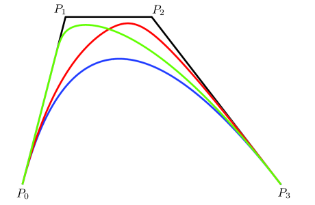
Figure 1: Gelfond-Bézier curves associated with the control polygon $(P_{0},P_{1},P_{2},P_{3})$ and Müntz spaces : blue curve $span(1,t,t^{2},t^{3})$, red curve $span(1,t,t^{2},t^{20})$, green curve $span(1,t^{2},t^{50},t^{100})$.

The derivative of the Gelfond-Bernstein Basis: We start with the following lemma giving the derivative of the divided differences

Lemma 2.

Le $x_{0},x_{1},...,x_{n}$ be pairwise distinct real numbers and consider the function $\psi(t)=[x_{0},x_{1},...,x_{n}]f_{t}$, where $f_{t}$ is the function defined as $f_{t}(x)=t^{x}$. Then we have

$$\psi^{\prime}(t)=x_{0}[x_{0}-1,x_{1}-1,...,x_{n}-1]f_{t}+[x_{1}-1,x_{2}-1,...,x_{n}-1]f_{t}.$$ (29)

Proof.

By the definition of the divided differences, we have

$$\psi^{\prime}(t)=\sum^{n}_{i=0}\frac{x_{i}t^{x_{i}-1}}{\prod^{n}_{j=0,j\neq i}{(x_{i}-x_{j})}}.$$ (30)

Now, the right hand side of the equation (29) is given by

$$x_{0}\sum^{n}_{i=0}\frac{t^{x_{i}-1}}{\prod^{n}_{j=0,j\neq i}{(x_{i}-x_{j})}}+\sum^{n}_{i=1}\frac{t^{x_{i}-1}}{\prod^{n}_{j=1,j\neq i}{(x_{i}-x_{j})}}.$$ (31)

Let $k$ be an integer in $\{0,1,...,n\}$ and let us compare the coefficient of the monomial $t^{x_{k}-1}$ in both of the expressions (30) and (31). For (30) the coefficient is given by

$$\frac{x_{k}}{\prod^{n}_{j=0,j\neq k}{(x_{k}-x_{j})}},$$

while for (31), the coefficient is given for $k=0$ by $\frac{x_{0}}{\prod^{n}_{j=0,j\neq 0}{(x_{0}-x_{j})}}$ and for $k\neq 0$ by

$$\frac{1}{\prod^{n}_{j=1,j\neq k}{(x_{k}-x_{j})}}\left(\frac{x_{0}}{x_{k}-x_{0}}+1\right)=\frac{x_{k}}{\prod^{n}_{j=0,j\neq k}{(x_{k}-x_{j})}}.$$

The equality of the coefficients conclude the proof of the lemma. ∎

A direct and simple consequence of the preceding lemma ( in which we omit the proof) is the following

Proposition 4.

Let $\Lambda=(0=r_{0},r_{1},...,r_{n})$ be a sequence of strictly increasing real numbers such that $r_{1}=1$, and let $H^{n}_{k,\Lambda},k=0,...,n$ be the Gelfond-Bernstein basis, over the interval $[0,1]$, associated with the Müntz space $E_{\Lambda}(n)$. Then, we have

$${H_{k,\Lambda}^{n}}^{\prime}(t)=\frac{\prod_{j=k+1}^{n}r_{j}}{\prod_{j=k+1}^{n}(r_{j}-1)}\left(r_{k}H^{n-1}_{k-1,\Lambda_{1}}(t)-(r_{k+1}-1)H^{n-1}_{k,\Lambda_{1}}(t)\right),$$

where is to be understood that

$${H_{0,\Lambda}^{n}}^{\prime}(t)=-\frac{\prod_{j=2}^{n}r_{j}}{\prod_{j=2}^{n}(r_{j}-1)}H^{n-1}_{0,\Lambda_{1}}(t)\quad\textnormal{;}\quad{H_{n,\lambda}^{n}}^{\prime}(t)=r_{n}H^{n}_{n,\Lambda_{1}}(t)$$

and $\Lambda_{1}$ is the sequence $\Lambda_{1}=(0=r_{0},r_{2}-1,r_{3}-1,...,r_{n}-1).$

From the last proposition, the following easily follows

Theorem 6.

Let $\Lambda=(0=r_{0},r_{1},...,r_{n})$ be a sequence of strictly increasing real numbers such that $r_{1}=1$ and consider the Gelfond-Bézier curve

$$P(t)=\sum_{k=0}^{n}H_{k,\Lambda}^{n}(t)P_{k}.$$

Then, we have

$$P^{\prime}(t)=\sum_{k=0}^{n-1}\frac{\prod_{j=k+1}^{n}r_{j}}{\prod_{j=k+2}^{n}(r_{j}-1)}H_{k,\Lambda_{1}}^{n-1}(t)\Delta{P_{k}},$$

where $\Lambda_{1}$ is the sequence $\Lambda_{1}=(0=r_{0},r_{2}-1,r_{3}-1,...,r_{n}-1)$. We adopt the convention that $\prod_{k=n+1}^{n}*=1$.

From the last theorem, we conclude that for sequences $\Lambda=(0=r_{0},r_{1},...,r_{n})$ such that $r_{1}=1$, the associated Gelfond-Bézier curves satisfy the tangency property at the end points, namely, we have

$$P^{\prime}(0)=\frac{\prod_{j=2}^{n}r_{j}}{\prod_{j=2}^{n}(r_{j}-1)}\Delta{P_{0}}\quad\textnormal{and}\quad P^{\prime}(1)=r_{n}\Delta{P_{n-1}}.$$

In the case we have a sequence $\Lambda=(0=r_{0},r_{1},...,r_{n})$ of strictly increasing real numbers such that $r_{1}>1$, then we can embed the Müntz space $E_{1}=span(1,t^{r_{1}},t^{r_{2}},...,t^{r_{n}})$ into the space $E_{2}=span(1,t,t^{r_{1}},t^{r_{2}},...,t^{r_{n}})$ in which the relation between the Gelfond-Bernstein bases of the spaces $E_{1}$ and $E_{2}$ is given in the forthcoming proposition 11. We can then apply proposition 4 to compute the derivatives of the Gelfond-Bernstein bases associated with the Müntz space $E_{2}$. Such a program, in which we omit the details due to their simplicity, leads to

Proposition 5.

Let $\Lambda=(0=r_{0},r_{1},...,r_{n})$ be a sequence of strictly increasing real numbers such that $r_{1}>1$ and let $H^{n}_{k,\Lambda},k=0,...,n$ be the Gelfond-Bernstein basis associated with the Müntz space $E_{\Lambda}(n)$. Then, we have, for $1\leq k\leq n-1$

$${H_{k,\Lambda}^{n}}^{\prime}(t)=\frac{\prod_{j=k+1}^{n}r_{j}}{\prod_{j=k+1}^{n}(r_{j}-1)}\left(r_{k}H^{n}_{k,\Lambda_{1}}(t)-(r_{k+1}-1)H^{n}_{k+1,\Lambda_{1}}(t)\right)$$

and

$${H_{0,\Lambda}^{n}}^{\prime}(t)=-\frac{\prod_{j=1}^{n}r_{j}}{\prod_{j=2}^{n}(r_{j}-1)}H^{n}_{1,\Lambda_{1}}(t)\quad\textnormal{and}\quad{H_{n,\Lambda}^{n}}^{\prime}(t)=r_{n}H^{n}_{n,\Lambda_{1}}(t),$$

where $\Lambda_{1}$ is the sequence $\Lambda_{1}=(0=r_{0},r_{1}-1,r_{2}-1,...,r_{n}-1)$.

From the last proposition, the following easily follows

Theorem 7.

Let $\Lambda=(0=r_{0},r_{1},...,r_{n})$ be a sequence of strictly increasing real numbers such that $r_{1}>1$ and consider the Gelfond-Bézier curve

$$P(t)=\sum_{k=0}^{n}H_{k,\Lambda}^{n}(t)P_{k}.$$

Then, we have

$$P^{\prime}(t)=\sum_{k=1}^{n}\frac{\prod_{j=k}^{n}r_{j}}{\prod_{j=k+1}^{n}(r_{j}-1)}H_{k,\Lambda_{1}}^{n}(t)\Delta{P_{k-1}},$$

where $\Lambda_{1}$ is the sequence $\Lambda_{1}=(0=r_{0},r_{1}-1,r_{2}-1,...,r_{n}-1)$.We adopt the convention that $\prod_{k=n+1}^{n}*=1$.

Note that from Theorem 7, we have $P^{\prime}(0)=0$. Therefore, for a sequence $\Lambda=(0=r_{0},r_{1},...,r_{n})$ of strictly increasing real numbers such that $r_{1}$ is a positive integer, we can iterate the statement of Theorem 7 to conclude that we have

$$P^{\prime}(0)=P^{(2)}(0)=...=P^{(r_{1}-1)}(0)=0\quad\textnormal{and}\quad P^{(r_{1})}(0)=\frac{\prod_{j=1}^{n}r_{j}}{\prod_{j=1}^{n}(r_{j}-r_{1})}\Delta P_{0},$$

thereby, showing that the Gelfond-Bézier curve is geometrically tangent to the control segment $[P_{0},P_{1}]$ for the parameter $t=0$. Moreover, we have $P^{\prime}(1)=r_{n}\Delta{P_{n-1}}$ showing that Gelfond-Bézier curves associated with sequences $\Lambda=(0=r_{0},r_{1},...,r_{n})$ of strictly increasing real numbers such that $r_{1}$ is a positive integer satisfy the tangency property at the end points.

6 Examples of Gelfond-Bernstein bases

For sequences $\Lambda=(0=r_{0},r_{1},...,r_{n})$ of strictly increasing integers, Proposition 3 gives an alternative method of deriving Gelfond-Bernstein bases of Müntz spaces using the combinatoric of Schur functions instead of computing with the divided differences. In this section, we will exhibit the usefulness of this approach by giving the Gelfond-Bernstein bases of some specific Müntz spaces. As horizontal, vertical and hook Young diagrams occupy an important place in the combinatorics of Schur functions, it is only natural to define the Müntz spaces associated with these particular Young diagrams and compute their Gelfond-Bernstein bases. We will also give one example of a low order Müntz space for a better emphazise on our main point. In section 2, we recalled several alternative way of computing Schur functions for integer partitions, such as the Jacobi-Trudi formula, the Nägelsbach-Kostka formula and the Giambelli formula. It is at this point of trying to derive explicit expressions of the Gelfond-Bernstein bases using Proposition 3 that the reader will feel the importance of these alternative way of computing Schur functions and our reason of reminding them. We will not fully exhibit this fact here, but the reader is invited to compute the Gelfond-Bernstein bases of more complicated Müntz spaces to be aware of the importance of the combinatorics of Schur functions. The same remarks apply to the computation of the blossom and the derivation of the de Casteljau algorithms in the next section. Notations 2: In notations 1, we have denoted as $E_{\Lambda}(n)$ or $\mathcal{E}_{\lambda}(n)$ the Müntz space $E=span(1,t^{r_{1}},t^{r_{2}},...,t^{r_{n}})$ so as to emphasize the sequence $\Lambda$ or the associated real partition $\lambda$ depending on the context. We will imitate these notations for the Gelfond-Bernstein basis of the Müntz space $E_{\Lambda}(n)=\mathcal{E}_{\lambda}(n)$, in which we denote them as $H^{n}_{k,\Lambda}$ or $\mathcal{H}^{n}_{k,\lambda}$ depending on the contextual emphasize. Polynomial Müntz space: Consider the Müntz space associated with the sequence $\Lambda=(0,1,2,...,n)$, namely the Müntz space $span(1,t,t^{2},...,t^{n})$. The partition $\lambda$ associated with the sequence $\Lambda$ is the empty partition, the bottom partition of $\lambda$ is also empty. Therefore, Theorem 3 states that the Gelfond-Bernstein basis associated with the sequence $\Lambda$ coincide with the classical Bernstein basis over the interval $[0,1]$. Combinatorial Müntz space: Consider the Müntz space $E_{\Lambda}(4)=span(1,t^{3},$ $t^{4},t^{6},t^{9})$ of order $4$. The sequence $\Lambda$ is given by $\Lambda=(r_{0}=0,r_{1}=3,r_{2}=4,r_{3}=6,r_{4}=9)$. The partition $\lambda$ associated with the sequence $\Lambda$ is given by $\lambda=(5,3,3,2)$. Let us, for example, compute the element $H^{4}_{2,\Lambda}$ of the Gelfond-Bernstein basis associated with the Müntz space $E_{\Lambda}(4)$. From proposition 3, we have

$$H^{4}_{2,\Lambda}(t)=\frac{\prod_{i=3}^{4}{r_{i}}}{\prod_{i=3}^{4}{(r_{i}-r_{2})}}t^{4}(1-t)^{2}\frac{\tiny S_{\hbox{}{\vbox{\offinterlineskip\vbox{\hrule height=0.3pt\hbox{\vrule height=3.06133pt,width=0.3pt,depth=0.76532pt\hbox to3.82666pt{\hfil}\vrule height=3.06133pt,width=0.3pt,depth=0.76532pt\hbox to3.82666pt{\hfil}\vrule height=3.06133pt,width=0.3pt,depth=0.76532pt\hbox to3.82666pt{\hfil}\vrule height=3.06133pt,width=0.3pt,depth=0.76532pt} \hrule height=0.3pt}\vspace{-\y@linethick} \vbox{\hrule height=0.3pt\hbox{\vrule height=3.06133pt,width=0.3pt,depth=0.76532pt\hbox to3.82666pt{\hfil}\vrule height=3.06133pt,width=0.3pt,depth=0.76532pt\hbox to3.82666pt{\hfil}\vrule height=3.06133pt,width=0.3pt,depth=0.76532pt} \hrule height=0.3pt}\vspace{-\y@linethick} }}}(1,t^{2})}{\tiny S_{\hbox{}{\vbox{\offinterlineskip\vbox{\hrule height=0.3pt\hbox{\vrule height=3.06133pt,width=0.3pt,depth=0.76532pt\hbox to3.82666pt{\hfil}\vrule height=3.06133pt,width=0.3pt,depth=0.76532pt\hbox to3.82666pt{\hfil}\vrule height=3.06133pt,width=0.3pt,depth=0.76532pt} \hrule height=0.3pt}\vspace{-\y@linethick} }}}(t^{2})}.$$

Therefore, using the branching rule (11), the expression of $H^{4}_{2,\Lambda}(t)$ is given by

$$\frac{27}{5}t^{4}(1-t)^{2}\frac{\tiny t^{3}f_{\hbox{}{\vbox{\offinterlineskip\vbox{\hrule height=0.3pt\hbox{\vrule height=3.06133pt,width=0.3pt,depth=0.76532pt\hbox to3.82666pt{\hfil}\vrule height=3.06133pt,width=0.3pt,depth=0.76532pt\hbox to3.82666pt{\hfil}\vrule height=3.06133pt,width=0.3pt,depth=0.76532pt\hbox to3.82666pt{\hfil}\vrule height=3.06133pt,width=0.3pt,depth=0.76532pt} \hrule height=0.3pt}\vspace{-\y@linethick} \vbox{\hrule height=0.3pt\hbox{\vrule height=3.06133pt,width=0.3pt,depth=0.76532pt\hbox to3.82666pt{\hfil}\vrule height=3.06133pt,width=0.3pt,depth=0.76532pt\hbox to3.82666pt{\hfil}\vrule height=3.06133pt,width=0.3pt,depth=0.76532pt} \hrule height=0.3pt}\vspace{-\y@linethick} }}}(2)+t^{2}(f_{\hbox{}{\vbox{\offinterlineskip\vbox{\hrule height=0.3pt\hbox{\vrule height=3.06133pt,width=0.3pt,depth=0.76532pt\hbox to3.82666pt{\hfil}\vrule height=3.06133pt,width=0.3pt,depth=0.76532pt\hbox to3.82666pt{\hfil}\vrule height=3.06133pt,width=0.3pt,depth=0.76532pt} \hrule height=0.3pt}\vspace{-\y@linethick} \vbox{\hrule height=0.3pt\hbox{\vrule height=3.06133pt,width=0.3pt,depth=0.76532pt\hbox to3.82666pt{\hfil}\vrule height=3.06133pt,width=0.3pt,depth=0.76532pt\hbox to3.82666pt{\hfil}\vrule height=3.06133pt,width=0.3pt,depth=0.76532pt} \hrule height=0.3pt}\vspace{-\y@linethick} }}}(2)+f_{\hbox{}{\vbox{\offinterlineskip\vbox{\hrule height=0.3pt\hbox{\vrule height=3.06133pt,width=0.3pt,depth=0.76532pt\hbox to3.82666pt{\hfil}\vrule height=3.06133pt,width=0.3pt,depth=0.76532pt\hbox to3.82666pt{\hfil}\vrule height=3.06133pt,width=0.3pt,depth=0.76532pt\hbox to3.82666pt{\hfil}\vrule height=3.06133pt,width=0.3pt,depth=0.76532pt} \hrule height=0.3pt}\vspace{-\y@linethick} \vbox{\hrule height=0.3pt\hbox{\vrule height=3.06133pt,width=0.3pt,depth=0.76532pt\hbox to3.82666pt{\hfil}\vrule height=3.06133pt,width=0.3pt,depth=0.76532pt} \hrule height=0.3pt}\vspace{-\y@linethick} }}}(2))+t(f_{\hbox{}{\vbox{\offinterlineskip\vbox{\hrule height=0.3pt\hbox{\vrule height=3.06133pt,width=0.3pt,depth=0.76532pt\hbox to3.82666pt{\hfil}\vrule height=3.06133pt,width=0.3pt,depth=0.76532pt\hbox to3.82666pt{\hfil}\vrule height=3.06133pt,width=0.3pt,depth=0.76532pt\hbox to3.82666pt{\hfil}\vrule height=3.06133pt,width=0.3pt,depth=0.76532pt} \hrule height=0.3pt}\vspace{-\y@linethick} }}}(2)+f_{\hbox{}{\vbox{\offinterlineskip\vbox{\hrule height=0.3pt\hbox{\vrule height=3.06133pt,width=0.3pt,depth=0.76532pt\hbox to3.82666pt{\hfil}\vrule height=3.06133pt,width=0.3pt,depth=0.76532pt\hbox to3.82666pt{\hfil}\vrule height=3.06133pt,width=0.3pt,depth=0.76532pt} \hrule height=0.3pt}\vspace{-\y@linethick} \vbox{\hrule height=0.3pt\hbox{\vrule height=3.06133pt,width=0.3pt,depth=0.76532pt\hbox to3.82666pt{\hfil}\vrule height=3.06133pt,width=0.3pt,depth=0.76532pt} \hrule height=0.3pt}\vspace{-\y@linethick} }}}(2))+f_{\hbox{}{\vbox{\offinterlineskip\vbox{\hrule height=0.3pt\hbox{\vrule height=3.06133pt,width=0.3pt,depth=0.76532pt\hbox to3.82666pt{\hfil}\vrule height=3.06133pt,width=0.3pt,depth=0.76532pt\hbox to3.82666pt{\hfil}\vrule height=3.06133pt,width=0.3pt,depth=0.76532pt} \hrule height=0.3pt}\vspace{-\y@linethick} }}}(2)}{\tiny f_{\hbox{}{\vbox{\offinterlineskip\vbox{\hrule height=0.3pt\hbox{\vrule height=3.06133pt,width=0.3pt,depth=0.76532pt\hbox to3.82666pt{\hfil}\vrule height=3.06133pt,width=0.3pt,depth=0.76532pt\hbox to3.82666pt{\hfil}\vrule height=3.06133pt,width=0.3pt,depth=0.76532pt} \hrule height=0.3pt}\vspace{-\y@linethick} }}}(2)}.$$

Using the hook length formula (7), we obtain

$$H^{4}_{2,\Lambda}(t)=\frac{27}{15}t^{4}(1-t)^{2}(3+6t+4t^{2}+2t^{3}).$$

Elementary Müntz spaces Let $l$ and $n$ be two positive integers such that $1\leq l\leq n$. Consider the Müntz space of order $n$, defined for $l\neq 1$ by $E=span(1,t,t^{2},...,t^{l-1},t^{l+1},...,t^{n+1})$ and $E=span(1,t^{2},t^{3},...,t^{n+1})$ for $l=1$. The partition $\lambda$ associated with the Müntz space $E$ is given by a vertical Young diagram with $l$ boxes, i.e, $\lambda=(1^{l})$. For this reason, we have called these Müntz spaces in [1] the $l$th elementary Müntz spaces. The sequence $\Lambda$ associated with $E$ is given by $\Lambda=(r_{0}=0,r_{1}=1,...,r_{l-1}=l-1,r_{l}=l+1,r_{l+1}=l+2,...,r_{n}=n+1)$. Let us first compute the Gelfond-Bernstein basis $\mathcal{H}^{n}_{k,(1^{l})}$ when $k\leq l-1$. In this case we have

$$\frac{\prod_{i=k+1}^{n}{r_{i}}}{\prod_{i=k+1}^{n}{(r_{i}-r_{k})}}=\frac{l-k}{l}\binom{n+1}{k}.$$

Therefore, by Proposition 3, for $k\leq l-1$, we have

$$\mathcal{H}^{n}_{k,(1^{l})}(t)=\frac{l-k}{l}\binom{n+1}{k}t^{k}(1-t)^{n-k}\frac{e_{l-k}(1,t^{n-k})}{e_{l-k-1}(t^{n-k})}.$$

Using the branching rule $e_{l-k}(1,t^{n-k})=e_{l-k}(t^{n-k})+e_{l-k-1}(t^{n-k})$, we obtain

$$\mathcal{H}^{n}_{k,(1^{l})}(t)=\frac{l-k}{l}\binom{n+1}{k}t^{k}(1-t)^{n-k}\left(1+\frac{n-l+1}{l-k}t\right).$$

For the case $k\geq l$, we have

$$\frac{\prod_{i=k+1}^{n}{r_{i}}}{\prod_{i=k+1}^{n}{(r_{i}-r_{k})}}=\binom{n+1}{k+1},$$

and then Proposition 3, gives

$$\mathcal{H}^{n}_{k,(1^{l})}(t)=\binom{n+1}{k+1}t^{k+1}(1-t)^{n-k}=B^{n+1}_{k+1}(t),$$

where $B^{n+1}_{k+1}$ is the classical Bernstein polynomials. Summarizing

Proposition 6.

The Gelfond-Bernstein basis of the elementary Müntz space $\mathcal{E}_{(1^{l})}(n)$ with respect to the interval $[0,1]$ is given by

$$\mathcal{H}^{n}_{k,(1^{l})}(t)=\frac{l-k}{l}\binom{n+1}{k}t^{k}(1-t)^{n-k}\left(1+\frac{n-l+1}{l-k}t\right)\quad\textnormal{for}\quad k=0,...,l-1$$

and

$$\mathcal{H}^{n}_{k,(1^{l})}(t)=B^{n+1}_{k+1}(t)\quad\textnormal{for}\quad k=l,...,n,$$

where $B^{n+1}_{k+1}$ is the classical Bernstein polynomials.

Complete Müntz spaces Let $l$ be a non-negative integer and consider the Müntz space of order $n$, $E=span(1,t^{l+1},...,t^{l+n})$. The partition associated with $E$ is given by a horizontal Young diagram with $l$ boxes, i.e., $\lambda=(l)$. For this reason, we call the Müntz space $E=\mathcal{E}_{(l)}(n)$ the $l$th complete Müntz space. The bottom partition $\lambda^{(0)}$ is an empty partition. The sequence $\Lambda$ is given by $\Lambda=(r_{0}=0,r_{1}=l+1,...r_{j}=l+j,...,r_{n}=l+n$. For any integer $0\leq k\leq n$, we have

$$\frac{\prod_{i=k+1}^{n}{r_{i}}}{\prod_{i=k+1}^{n}{(r_{i}-r_{k})}}=\binom{n+l}{k+l}\;\textnormal{if}\;k\neq 0\quad\textnormal{and}\quad\frac{\prod_{i=k+1}^{n}{r_{i}}}{\prod_{i=k+1}^{n}{(r_{i}-r_{k})}}=1\;\textnormal{if}\;k=0.$$

Therefore, by Proposition 3, we have

$$\mathcal{H}^{n}_{0,(l)}(t)=(1-t)^{n}h_{l}(1,t^{n})$$

and

$$\mathcal{H}^{n}_{k,(l)}(t)=\binom{n+l}{k+l}t^{l+k}(1-t)^{n-k}=B^{n+l}_{k+l}(t)\quad\textnormal{for}\quad k=1,...,n.$$

Summarizing,

Proposition 7.

The Gelfond-Bernstein basis of the complete Müntz space $\mathcal{E}_{(l)}(n)$ with respect to the interval $[0,1]$ is given by

$$\mathcal{H}^{n}_{0,(l)}(t)=(1-t)^{n}\sum_{j=0}^{l}\binom{n+j-1}{n-1}t^{j}$$

and

$$\mathcal{H}^{n}_{k,(l)}(t)=B^{n+l}_{k+l}(t)\quad\textnormal{for}\quad k=1,...,n,$$

where $B^{n+l}_{k+l}$ is the classical Bernstein basis.

Hook Müntz spaces: Let $l$ and $n$ be two positive integers and let $m$ be a positive integer such that $0<m<n$. Consider the Müntz space of order $n$, $E=span(1,t^{l+1},t^{l+2},...,t^{l+m},t^{l+m+2},...,t^{l+n+1})$. The partition $\lambda$ associated with the space $E$ is given by a $(l,m)$-hook Young diagram, i.e., $\lambda=(l|m)$. Therefore, we call the space $E=\mathcal{E}_{(l|m)}(n)$ the $(l|m)$-hook Müntz space. For $k=0$, Proposition 3 gives

$$\mathcal{H}^{n}_{0,(l|m)}(t)=(1-t)^{n}\frac{S_{(l|m)}(1,t^{n})}{e_{m}(t^{n})}.$$

The branching rule (12) leads to

$$S_{(l|m)}(1,t^{n})=S_{(l|m)}(t^{n})+e_{m}(t^{n})\sum_{j=1}^{l+1}h_{l+1-j}(t^{n}).$$

Therefore,

$$\frac{S_{(l|m)}(1,t^{n})}{e_{m}(t^{n})}=\frac{1}{f_{(1^{m})}(n)}\left(t^{l+1}f_{(l|m)}(n)+\sum_{j=1}^{l+1}f_{(l+1-j)}(n)t^{l+1-j}\right),$$ (32)

in which the terms expressing the hook lengths can be computed using equations (8) and (9). For $k\leq m$, we have

$$\frac{\prod_{i=k+1}^{n}{r_{i}}}{\prod_{i=k+1}^{n}{(r_{i}-r_{k})}}=\frac{m+1-k}{m+1+l}\binom{l+n+1}{l+k}.$$

Therefore, Proposition 3 gives

$$\mathcal{H}^{n}_{k,(l|m)}(t)=\frac{m+1-k}{m+1+l}\binom{l+n+1}{l+k}t^{l+k}(1-t)^{n-k}\frac{e_{m-k+1}(1,t^{n-k})}{e_{m-k}(t^{n-k})}.$$

Using the branching rule for the elementary symmetric functions leads to

$$\mathcal{H}^{n}_{k,(l|m)}(t)=\frac{m+1-k}{m+1+l}\binom{l+n+1}{l+k}t^{l+k}(1-t)^{n-k}\left(\frac{(n-m)t}{m-k+1}+1\right).$$

For $k>m$, we have

$$\frac{\prod_{i=k+1}^{n}{r_{i}}}{\prod_{i=k+1}^{n}{(r_{i}-r_{k})}}=\binom{l+n+1}{l+k+1}.$$

Thus, the corresponding Gelfond-Bernstein element is given by

$$\mathcal{H}^{n}_{k,(l|m)}(t)=\binom{l+n+1}{l+k+1}t^{l+k+1}(1-t)^{n-k}=B^{l+n+1}_{l+k+1}(t).$$

Summarizing

Proposition 8.

The Gelfond-Bernstein basis of the hook Müntz space $\mathcal{E}_{(l|m)}(n)$ with respect to the interval $[0,1]$ is given by

$$\mathcal{H}^{n}_{0,(l|m)}(t)=(1-t)^{n}\frac{S_{(l|m)}(1,t^{n})}{e_{m}(t^{n})},$$

where an explicit expression of the Schur functions can be computed using (32). For $k=1,..,m$

$$\mathcal{H}^{n}_{k,(l|m)}(t)=\frac{m+1-k}{m+1+l}\binom{l+n+1}{l+k}t^{l+k}(1-t)^{n}\left(\frac{(n-m)t}{m-k+1}+1\right)$$

and for $k=m+1,...,n$

$$\mathcal{H}^{n}_{k,(l|m)}(t)=B^{l+n+1}_{l+k+1}(t),$$

where $B^{n+l+1}_{l+k+1}$ is the classical Bernstein basis.

7 Blossom and the de Casteljau algorithms

As the Gelfond-Bernstein bases are limits of the Chebyshev-Bernstein bases in Müntz spaces, we can extend the notion of blossom to the Gelfond-Bézier curves using Theorem 1, which in turn will allows us to derive the corresponding de Casteljau algorithms

Definition 5.

Let $\Lambda=(0=r_{0},r_{1},...,r_{n})$ be a sequence of strictly increasing real numbers and let $\lambda=(\lambda_{1},...,\lambda_{n})$ be the associated real partition. Consider an element $P$ of the Müntz space $E_{\Lambda}(n)=\mathcal{E}_{\lambda}(n)$ written as

$$P(t)=\sum_{k=0}^{n}a_{k}t^{r_{k}}.$$

Then, the blossom $f_{P}$ of $P$ is defined for any $0\leq j\leq n-1$ and $u_{j+1},...,u_{n}$ in $]0,1]$ by

$$f_{P}(0^{j},u_{j+1},...,u_{n})=a_{0}+\lim_{\epsilon\to 0}\sum_{k=0}^{n}a_{k}\frac{f_{\lambda^{(0)}}(n)}{f_{\lambda^{(k)}}(n)}\frac{S_{\lambda^{(k)}}(\epsilon^{j},u_{j+1},...,u_{n})}{S_{\lambda^{(0)}}(\epsilon^{j},u_{j+1},...,u_{n})},$$

where $(\lambda^{(0)},\lambda^{(1)},...,\lambda^{(n)})$ is the Müntz tableau associated with the partition $\lambda$, and $f_{P}(0^{n})=a_{0}$.

It is clear from the definition that the blossom $f_{P}$ is symmetric in its arguments and that for any $t\in[0,1]$, $f_{P}(t,t,...,t)=P(t)$. Moreover, if we express the function $P$ in the Gelfond-Bernstein basis as

$$P(t)=\sum_{k=0}^{n}p_{k}\mathcal{H}^{n}_{k,\lambda}(t)$$

then, the values $p_{k},k=0,...,n$ are given by

$$p_{k}=f_{P}(0^{n-k},1^{k}).$$

Therefore, to compute the control points of the function $P$ over the interval $[0,1]$, we need only to compute the control points of the functions $t^{r_{k}}$, $k=1,...,n$. Such computation is given in the following

Proposition 9.

Let $\mathcal{H}^{n}_{k,\lambda},k=0,,...,n$ be the Gelfond-Bernstein basis of the Müntz space $\mathcal{E}_{\lambda}(n)=span(1,t^{r_{1}},...,t^{r_{n}})$. Then, we have

$$t^{r_{k}}=\sum_{j=k}^{n}p_{j}\mathcal{H}^{n}_{j,\lambda}(t),$$

where

$$p_{j}=(1-\frac{r_{k}}{r_{j+1}})(1-\frac{r_{k}}{r_{j+2}})...(1-\frac{r_{k}}{r_{n}})\quad\textnormal{for}\quad j=k,...,n-1$$ (33)

and

$$p_{n}=1.$$

Proof.

Let us choose $1\leq k\leq n-1$, and denote by $p_{j}$ the $j$th control point of the function $t^{r_{k}}$. From the definition of the blossom, we have

$$p_{j}=\frac{f_{\lambda^{(0)}}(n)}{f_{\lambda^{(k)}}(n)}\lim_{\epsilon\to 0}\frac{S_{\lambda^{(k)}}(1^{j},\epsilon^{n-j})}{S_{\lambda^{(0)}}(1^{j},\epsilon^{n-j})}.$$

As $\lambda^{(k)}=(\lambda_{1}+1,\lambda_{2}+1,...,\lambda_{k}+1,\lambda_{k+2},...,\lambda_{n},0)$ and $\lambda^{(0)}=(\lambda_{2},\lambda_{3},...,\lambda_{n},0)$, it is clear from the splitting formula (13) that if $j<k$ then $p_{j}=0$. In the case $j\geq k$, then again by the splitting formula (13), we have

$$p_{j}=\frac{f_{\lambda^{(0)}}(n)}{f_{\lambda^{(k)}}(n)}\frac{f_{\mu}(j)}{f_{\eta}(j)},$$

where $\mu$ and $\eta$ are the real partitions

$$\mu=(\lambda_{1}+1,\lambda_{2}+1,...,\lambda_{k}+1,\lambda_{k+2},...,\lambda_{j+1})$$

and

$$\eta=(\lambda_{2},\lambda_{3},...,\lambda_{k},\lambda_{k+1},...,\lambda_{j+1}).$$

Lengthy, yet straightforward computations, using the hook length formula (10), shows that $p_{j}$ is given by (33). The case $k=n$ is straightforward. ∎

Remark 1.

Note that in the polynomial case $\mathcal{E}_{\emptyset}(n)=span(1,t,t^{2},...,t^{n})$, the last proposition give the familiar fact that the $j$th control point $p_{j}$ of the function $t^{k}$ is zero if $j<k$ and for $j\geq k$, we have

$$p_{j}=(1-\frac{k}{j+1})(1-\frac{k}{j+2})...(1-\frac{k}{n})=\frac{\binom{j}{k}}{\binom{n}{k}}.$$

Remark 2.

Proposition 9 can also be proven without resorting to the notion of blossoming, but instead using the Cauchy residue formula as in [8]. For the seek of comparison, and of bringing up front a different aspect in the theory of Gelfond-Bernstein bases, we will include the main steps of the proof here. For a sequence $\Lambda=(0=r_{0},r_{1},...,r_{n})$ of strictly increasing real numbers and using the Cauchy residue formula in can be easily shown that the Gelfond-Bernstein basis $H^{n}_{k,\Lambda},k=0,..,n$ associated with the sequence $\Lambda$ can be expressed (for $0\leq k\leq n-1$) as

$$H^{n}_{k,\Lambda}(t)=(-1)^{n-k}r_{k+1}...r_{n}\frac{1}{2\pi i}\int_{\Gamma}\frac{t^{z}}{(z-r_{k})(z-r_{k+1})...(z-r_{n})}dz,$$ (34)

where $\Gamma$ is any simple closed curve that contains the nodes $r_{i},i=k,...,n$ in its interior $Int(\Gamma)$, and such that the function $t^{z}$ is holomorphic in a neighborhood of $Int(\Gamma)\cup\Gamma$. Let us fix a $k<n$, then it can be proven by induction on $n$ that $1/z-r_{k}$ can also be written as

$$\frac{1}{z-r_{n}}-\frac{r_{n}-r_{k}}{(z-r_{n-1})(z-r_{n})}+...+(-1)^{n-k}\frac{(r_{k+1}-r_{k})(r_{k+2}-r_{k})...(r_{n}-r_{k})}{(z-r_{k})(z-r_{k+1})...(z-r_{n})}.$$

Multiplying the last equation as well as the function $1/z-r_{k}$ by $t^{z}/2\pi i$ and integrating over $\Gamma$ leads, after using equation (34), to a new proof of Proposition 9.

To express the pseudo-affinity property of the blossom in the space $\mathcal{E}_{\lambda}(n)$ over the interval $[0,1]$, we can just introduce the following pseudo-affinity factor

Definition 6.

Let $\lambda=(\lambda_{1},\lambda_{2},...,\lambda_{n})$ be a real partition, and let $c,d$ be two real numbers in the interval $[0,1]$ such that $c<d$. we define the function $\alpha$ by: for any $0\leq j\leq n-1$ and $U=(u_{j+1},...,u_{n-1})$ in $]0,1]$ if $c\neq 0$

$$\alpha(0^{j},U;c,d,t)=\lim_{\epsilon\to 0}\frac{t-c}{d-c}\frac{S_{\lambda}(\epsilon^{j},U,c,t)S_{\lambda^{(0)}}(\epsilon^{j},U,d)}{S_{\lambda}(\epsilon^{j},U,c,d)S_{\lambda^{(0)}}(\epsilon^{j},U,t)},$$

while for $c=0$, we define $\alpha$ as

$$\alpha(0^{j},U;0,d,t)=\lim_{\epsilon\to 0}\frac{t}{d}\frac{S_{\lambda}(\epsilon^{j+1},U,t)S_{\lambda^{(0)}}(\epsilon^{j},U,d)}{S_{\lambda}(\epsilon^{j+1},U,d)S_{\lambda^{(0)}}(\epsilon^{j},U,t)},$$ (35)

where $\lambda^{(0)}$ is the bottom partition of $\lambda$.

Taking the limit in the pseudo-affinity factor in Theorem 2 of the Chebyshev blossom shows that the blossom of Gelfond-Bézier curves satisfies the following pseudo-affinity property : If for a function $P$ in the Müntz space $\mathcal{E}_{\lambda}(n)$, we denote by $f_{P}$ its blossom, then for any $U=(u_{1},...,u_{n-1})$, sequence of real numbers in $[0,1]$, we have

$$f_{P}(U,t)=(1-\alpha(U;c,d,t))f_{P}(U,c)+\alpha(U;c,d,t).f_{P}(U,d)$$

In order to derive the de Casteljau algorithm associated with the Müntz space $\mathcal{E}_{\lambda}(n)$ over the interval $[0,1]$, we should derive the pseudo-affinity factor when $c=0$ and $d=1$. According to (35) , we have

$$\alpha(0^{j},U;0,1,t)=\lim_{\epsilon\to 0}t\frac{S_{\lambda}(\epsilon^{j+1},U,t)S_{\lambda^{(0)}}(\epsilon^{j},U,1)}{S_{\lambda}(\epsilon^{j+1},U,1)S_{\lambda^{(0)}}(\epsilon^{j},U,t)}.$$

Applying the splitting formula (13) leads to

Proposition 10.

Let $\lambda=(\lambda_{1},...,\lambda_{n}$) be a real partition. Then, the pseudo-affinity factor of the space $\mathcal{E}_{\lambda}(n)$ is given, for $j\leq n-1$, by

$$\alpha(0^{j},U;0,1,t)=t\frac{S_{\mu}(U,t)S_{\eta}(U,1)}{S_{\mu}(U,1)S_{\eta}(U,t)},$$

where $\mu=(\lambda_{1},\lambda_{2},...,\lambda_{n-j})$ and $\eta=(\lambda_{2},\lambda_{3},...,\lambda_{n-j+1}).$

de Casteljau algorithm for elementary Müntz spaces: In the following, we derive the de Casteljau algorithm for the elementary Müntz spaces. We first study two special cases, namely, the Müntz space associated with the partition $\lambda=(1^{n})$, i.e, the space $\mathcal{E}_{(1^{n})}(n)=span(1,t,t^{2},...,t^{n-1},t^{n+1})$ and the Müntz space associated with the partition $\lambda=(1)$, i.e.; the space $span(1,t^{2},...,t^{n},t^{n+1})$. For the space $\mathcal{E}_{(1^{n})}$ and according to Proposition 10, the pseudo-affinity factor is given, for $j\neq 0$, by

$$\alpha(0^{j},U;0,1,t)=t\frac{e_{n-j}(U,t)e_{n-j}(U,1)}{e_{n-j}(U,1)e_{n-j}(U,t)}=t,$$

while for $j=0$, we have

$$\alpha(U;0,1,t)=t\frac{e_{n}(U,t)e_{n-1}(U,1)}{e_{n}(U,1)e_{n-1}(U,t)}=t^{2}\frac{e_{n-1}(U,1)}{e_{n-1}(U,t)}.$$

The last equations lead to the following de Casteljau algorithm for $\mathcal{E}_{(1^{n})}(n)$, in which for simplicity we exhibit the case of a Gelfond-Bézier curve of order $3$ with control points $(p_{0},p_{1},p_{2},p_{3})$ over the interval $[0,1]$ (Figure 2), as follows

where $x_{i}$, $i=1,2,3$ are given by

$$x_{i}=t^{2}\frac{e_{2}(t^{i-1},1^{3-i+1})}{e_{2}(t^{i},1^{3-i})}.$$

In the general case, the de Casteljau algorithm of the Müntz space $\mathcal{E}_{(1^{n})}(n)$ is given by:

Given $p_{i}^{0}=p_{i}$, $i=0,...,n$

for $r=1:n$ do

for $i=0:n-r-1$ do

$p_{i}^{r}=(1-t)p_{i}^{r-1}+tp_{i+1}^{r-1}$

$$\hskip-122.34692ptx_{r}=t^{2}\frac{e_{n-1}(t^{r-1},1^{n-r+1})}{e_{n-1}(t^{r},1^{n-r})}$$

$p_{n-r}^{r}=(1-x_{r})p_{n-r}^{r-1}+x_{r}p_{n-r+1}^{r-1}$

return

return

$P(t)=p_{0}^{n}$.

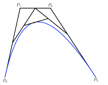
Figure 2: The de Casteljau algorithm for the Müntz space $\mathcal{E}_{(1^{3})}(3)=span(1,t,t^{2},t^{4})$ applied to the Gelfond-Bézier curves associated with the control polygon $(P_{0},P_{1},P_{2},P_{3})$ for the parameter $t=1/2$.

Remark 3.

The phenomena that at each level of the de Casteljau algorithm only the edges of the last triangle has weights that are different from the classical de Casteljau algorithm is not specific to this case but the same phenomena appears for all Müntz spaces associated with partitions of the shape $\lambda=(r^{n})$ where $r$ is a real number, namely, Müntz spaces $span(1,t,t^{2},...,t^{n-1},t^{s})$ where $s$ is a real number strictly larger than $n-1$.

Consider, now, the pseudo-affinity factor associated with the Müntz space $\mathcal{E}_{(1)}(n)$. According to proposition 10, we have

$$\alpha(0^{j},U;0,1,t)=t\frac{e_{1}(U,t)}{e_{1}(U,1)}.$$

The last equation leads to the following de Casteljau algorithm for $\mathcal{E}_{(1)}(n)$, in which again for simplicity we exhibit the case of a Gelfond-Bézier curve of order $3$ with control points $(p_{0},p_{1},p_{2},p_{3})$ over the interval $[0,1]$ (Figure 3), as follows

In the general case the de Casteljau algorithm of the Müntz space $\mathcal{E}_{(1)}(n)$ is given by :

Given $p_{i}^{0}=p_{i}$, $i=0,...,n$

for $r=1:n$ do

for $i=0:n-r$ do

$$\hskip-7.39755ptp_{i}^{r}=(1-\frac{rt^{2}+it}{(r-1)t+(i+1)})p_{i}^{r-1}+\frac{rt^{2}+it}{(r-1)t+(i+1)}p_{i+1}^{r-1}$$

return

return

$P(t)=p_{0}^{n}$.

In the general case of elementary Müntz space $\mathcal{E}_{(1^{r})}(n)$, the pseudo-affinity factor is given, for $j\geq n-r+1$, by

$$\alpha(0^{j},U;0,1,t)=t\frac{e_{n-j}(U,t)e_{n-j}(U,1)}{e_{n-j}(U,1)e_{n-j}(U,t)}=t,$$

while for $j<n-r+1$, we have

$$\alpha(U;0,1,t)=t\frac{e_{r}(U,t)e_{r-1}(U,1)}{e_{r}(U,1)e_{r-1}(U,t)}.$$

We leave it as an exercise, to the reader, to derive the de Casteljau algorithm of the $r$th elementary Müntz space from the last equations.

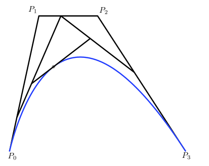
Figure 3: The de Casteljau algorithm for the Müntz space $\mathcal{E}_{(1)}(3)=span(1,t^{2},t^{3},t^{4})$ applied to the Gelfond-Bézier curves associated with the control polygon $(P_{0},P_{1},P_{2},P_{3})$ for the parameter $t=1/2$.

de Casteljau algorithm for complete Müntz spaces: From proposition 10, the pseudo-affinity factor of the $k$th complete Müntz space is given by

$$\alpha(0^{j},U;0,1,t)=t\frac{h_{k}(U,t)}{h_{k}(U,1)}.$$

The last equation leads to the following de Casteljau algorithm for $\mathcal{E}_{(k)}(n)$, in which for simplicity we exhibit the case of a Gelfond-Bézier curve of order $3$ with control points $(p_{0},p_{1},p_{2},p_{3})$ over the interval $[0,1]$ (Figure 4), as follows

In the general case the de Casteljau algorithm of the Müntz space $\mathcal{E}_{(k)}(n)$ is given by :

Given $p_{i}^{0}=p_{i}$, $i=0,...,n$

for $r=1:n$ do

for $i=0:n-r$ do

$$\hskip-28.45274ptp_{i}^{r}=\left(1-\frac{th_{k}(1^{i},t^{r})}{h_{k}(1^{i+1},t^{r-1})}\right)p_{i}^{r-1}+\frac{th_{k}(1^{i},t^{r})}{k_{k}(1^{i+1},t^{r-1})}p_{i+1}^{r-1}$$

return

return

$P(t)=p_{0}^{n}$.

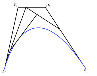
Figure 4: The de Casteljau algorithm for the Müntz space $\mathcal{E}_{(2)}(3)=span(1,t^{3},t^{4},t^{5})$ applied to the Gelfond-Bézier curves associated with the control polygon $(P_{0},P_{1},P_{2},P_{3})$ for the parameter $t=1/2$.

Remark 4.

Let $\lambda$ be a real partition associated with a Müntz space of order $n$, $\mathcal{E}_{\lambda}(n)$, and let $P$ be an element of $\mathcal{E}_{\lambda}(n)$ written in the Gelfond-Bernstein basis as

$$P(t)=\sum_{j=0}^{n}p_{j}\mathcal{H}^{n}_{j,\lambda}(t).$$

Denote by $q_{i},i=0,...,n$ the control points of the function $P$ over an interval $[a,b]$ such that $0<a<b<1$, namely $q_{i}=f_{P}(a^{n-i},b^{i})$. Then from the properties of the blossom, the function $P$ can also be written as

$$P(t)=\sum_{j=0}^{n}q_{j}B^{n}_{j,\lambda}(t),$$

where $B^{n}_{j,\lambda},j=0,...,n$ is the Chebyshev-Bernstein basis of the space $\mathcal{E}_{\lambda}(n)$ over the interval $[a,b]$. Therefore, in some sense, the Gelfond-Bernstein basis over an interval contained in $[0,1]$ and does not contain the origin is exactly the Chebyshev-Bernstein basis. This has the drawback that if we reiterate the de Casteljau algorithm over intervals that does not contain the origin then we loose the simplifications in the algorithm that were brought up by the origin through the splitting principle of Schur functions. To ovoid this drawback in practice, we should always make sure that the origin is a part of our interval. For example, to draw Gelfond-Bézier curves using the de Casteljau algorithm, we first subdivide the interval $[0,1]$ into the desired number of sub-intervals $[0=x_{0},x_{1}],[x_{1},x_{2}],....,[x_{m-1},x_{m}=1]$ and then apply successively the de Casteljau algorithm over the intervals $[0,x_{s}]\cup[x_{s},x_{s+1}]$ for $s=m-1,m-2,...,1$.

8 The dimension elevation process

Let $\Lambda_{1}=(0=r_{0},r_{1},...,r_{n})$ be a sequence of strictly increasing real numbers and let $H^{n}_{k,\Lambda_{1}}(t)$ be its corresponding Gelfond-Bernstein basis. Consider, now, a real number $\rho\neq r_{i},i=0,...,n$. The Müntz space $E_{\Lambda_{1}}(n)$ is a subset of the Müntz space $E=span(1,t^{r_{1}},...,t^{r_{n}},t^{\rho})$. Therefore, the Gelfond-Bernstein basis of the space $E_{\Lambda_{1}}(n)$ can be expressed in terms of the Gelfond-Bernstein basis of the space $E$. Such expressions depend on the position of $\rho$ in the sequence $r_{1}<r_{2}<...<r_{n}$ with respect to the increasing order. If we denote by $\Lambda_{2}$ the sequence obtained by arranging $(r_{0}=0,r_{1},...,r_{n},\rho)$ in a strictly increasing order, then we have

Proposition 11.

If $\rho>r_{n}$, then for $k=0,...,n$, we have

$$H^{n}_{k,\Lambda_{1}}(t)=\frac{\rho-r_{k}}{\rho}H^{n+1}_{k,\Lambda_{2}}(t)+\frac{r_{k+1}}{\rho}H^{n+1}_{k+1,\Lambda_{2}}(t).$$ (36)

If $\rho<r_{1}$, then

$$H^{n}_{0,\Lambda_{1}}(t)=H^{n+1}_{0,\Lambda_{2}}(t)+H^{n+1}_{1,\Lambda_{2}}(t)$$

and for $k\geq 1$, we have

$$H^{n}_{k,\Lambda_{1}}(t)=H^{n+1}_{k+1,\Lambda_{2}}(t).$$

If for a certain $s$, we have $r_{s}<\rho<r_{s+1}$, then for $k\geq s$, we have

$$H^{n}_{k,\Lambda_{1}}(t)=H^{n+1}_{k+1,\Lambda_{2}}(t).$$

$$H^{n}_{s-1,\Lambda_{1}}(t)=\frac{\rho-r_{s-1}}{\rho}H^{n+1}_{s-1,\Lambda_{2}}(t)+H^{n+1}_{s,\Lambda_{2}}(t)$$

and for $k<s-1$

$$H^{n}_{k,\Lambda_{1}}(t)=\frac{\rho-r_{k}}{\rho}H^{n+1}_{k,\Lambda_{2}}(t)+\frac{r_{k+1}}{\rho}H^{n+1}_{k+1,\Lambda_{2}}(t).$$

Proof.

We will only prove (36), as the other cases can be proven similarly. From the definition of the Gelfond-Bernstein basis, the right hand side of equation (36) is given by (for $k\leq n-1$)

$$(-1)^{n-k}r_{k}r_{k+1}...r_{n}\left([r_{k+1},...,\rho]f_{t}-(\rho-r_{k})[r_{k},...,\rho]f_{t}\right).$$ (37)

From the definition of the divided difference, we have

$$[r_{k+1},...,\rho]f_{t}-[r_{k},...,r_{n}]f_{t}=(\rho-r_{k})[r_{k},...,\rho]f_{t}.$$

Inserting the last equation into (37) conclude the proof of the lemma for $k\leq n-1$. For $k=n$, the left hand side of (36) is equal to

$$t^{\rho}-(\rho-r_{n})[r_{n},\rho]f_{t}=t^{r_{n}}=H^{n}_{n,\Lambda_{1}}(t).$$

∎

Consider now an element of $E_{\Lambda_{1}}(n)$, written in the Gelfond-Bernstein bases of the spaces $E_{\Lambda_{1}}(n)$ and $E_{\Lambda_{2}}(n+1)$ as

$$P(t)=\sum_{k=0}^{n}H_{k,\Lambda_{1}}^{n}(t)P_{k}=\sum_{k=0}^{n+1}H_{k,\Lambda_{2}}^{n+1}(t)\tilde{P}_{k},$$ (38)

where $\Lambda_{1}$ and $\Lambda_{2}$ refer to the sequences in the statement of the last proposition. Using proposition 11 to detect the coefficients of $H_{k,\Lambda_{2}}^{n+1}(t)$ in the expansion (38), we readily find

Corollary 3.

The Gelfond-Bézier points $\tilde{P_{k}}$ in (38) are related to the Gelfond-Bézier points $P_{k}$ by the relations

$$\tilde{P}_{0}=P_{0},\quad\tilde{P}_{n+1}=P_{n},$$

and if $\rho>r_{n}$ then for $k=1,2,...,n$

$$\tilde{P}_{k}=\frac{r_{k}}{\rho}\;P_{k-1}+\frac{(\rho-r_{k})}{\rho}\;P_{k}.$$ (39)

If $\rho<r_{1}$ then for $k=0,...,n-1$, we have

$$\tilde{P}_{k+1}=P_{k},$$

and if for an $s$, we have $r_{s}<\rho<r_{s+1}$, then for $k=1,2,...,s-1$

$$\tilde{P}_{k}=\frac{r_{k}}{\rho}\;P_{k-1}+\frac{(\rho-r_{k})}{\rho}\;P_{k},$$

and for $k=s,...,n+1$

$$\tilde{P}_{k}=P_{k-1}.$$

Let $n$ be a fixed integer and let $(0=r_{0},r_{1},...,r_{n},r_{n+1},....,r_{m},...)$ be an infinite sequence of strictly increasing real numbers. For any positive integer $q$, we denote by $\Lambda_{q}=(0=r_{0},r_{1},...,r_{q})$. Let $P$ be an element of the Müntz space $E_{\Lambda_{n}}(n)$ written as

$$P(t)=\sum_{k=0}^{n}H_{k,\Lambda_{n}}^{n}(t)P_{k}=\sum_{k=0}^{m}H_{k,\Lambda_{m}}^{m}(t)\tilde{P}_{k};\quad m>n.$$ (40)

Then, from corollary 3, equation (39), the control points $\tilde{P}_{k}$ can be computed using the following corner cutting scheme : For $i=0,1,...,n$, we set $P_{i}^{0}=P_{i}$ and for $j=1,2,...m-n$, we construct iteratively new polygons $(P_{0}^{j},P_{1}^{j},....,P_{n+j}^{j})$ using the inductive rule

$$P_{0}^{j}=P_{0}^{j-1}\quad P_{n+j}^{j}=P_{n+j-1}^{j-1}$$ (41)

and for $i=1,...,n+j-1$

$$P_{i}^{j}=\frac{r_{i}}{r_{n+j}}P_{i-1}^{j-1}+\left(1-\frac{r_{i}}{r_{n+j}}\right)P_{i}^{j-1}.$$ (42)

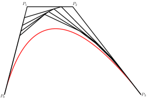
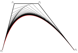
Figure 5: The sequence of polygons generated by the corner cutting scheme (41) and (42) and parameters $n=3,r_{1}=1,r_{2}=2,r_{3}=3$ and $r_{j}=2j$ for $j\geq 4$. (left, four iterations of the scheme; right, 100 iterations of the scheme). The red curve is the Bézier curve associated with the control polygon $(P_{0},P_{1},P_{2},P_{3})$.

In the case $r_{i}=i$ for any integer $i$, then we obtain the degree elevation algorithm, in which it is well know that the generated control polygon converges to the underlying Bézier curve as $m$ goes to infinity [14]. Now consider the case in which $r_{i}=i$ for $i=1,...,n$ and $r_{i}=2i$ for $i>n$. Figure 5 (left) shows the generated polygons from the scheme (41) and (42) from four iterations, while Figure 5 (right) shows the generated polygons from 100 iterations. The figure suggests the convergence of the generated polygons to the Bézier curve with control points $(P_{0},P_{1},...P_{n})$. Consider, now, the case in which $r_{i}=i$ for $i=1,...,n$, while $r_{i}=i^{2}$ for $i>n$. Figure 6 (left) shows the generated polygons from four iterations, while Figure 6 (right) shows the obtained polygons after 100 iterations. It is clear from the figure that the limiting polygon does not converge to the Bézier curve with control points $(P_{0},P_{1},...,P_{n})$. Now, consider, for example, the limiting polygon of the corner cutting scheme (41) and (42) for the case $n=3$ and in which $r_{1}=2,r_{2}=4,r_{3}=5$ and $r_{i}=2i$ for $i>3$.

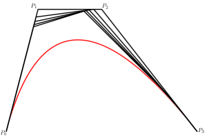
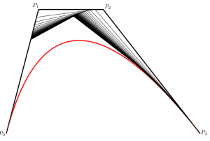
Figure 6: The sequence of polygons generated by the corner cutting scheme (41) and (42) and parameters $n=3,r_{1}=1,r_{2}=2,r_{3}=3$ and $r_{j}=j^{2}$ for $j\geq 4$. (left, four iterations of the scheme; right, 100 iterations of the scheme). The red curve is the Bézier curve associated with the control polygon $(P_{0},P_{1},P_{2},P_{3})$.

Figure 7 shows the generated polygons from 100 iterations and also shows the Gelfond-Bézier curve associated with the Müntz space $F=span(1,t^{r_{1}},t^{r_{2}},t^{r_{3}})=span(1,t^{2},t^{4},t^{5})$ and control polygon $(P_{0},P_{1},P_{2},P_{3})$. The figure suggests that the limiting polygon converges to the Gelfond-Bézier curve. In fact, in [2], the following was proven

Theorem 8.

Let $n$ be a fixed number and let $0<r_{1}<r_{2}<...r_{n}<r_{n+1}<...<{r_{m}}<...$ be an infinite strictly increasing sequence of positive real numbers such that $\lim_{s\to\infty}r_{s}=\infty$. Then the limiting polygon generated from a polygon $(P_{0},P_{1},...,P_{n})$ in $\mathbb{R}^{s},s\geq 1$ using the corner cutting scheme (41) and (42) converges (pointwise and uniformly) to the Gelfond-Bézier curve associated with the Müntz space $span(1,t^{r_{1}},t^{r_{2}},...,t^{r_{n}})$ and control polygon $(P_{0},P_{1},...,P_{n})$ if and only if the real number $r_{i}$ satisfy the condition

$$\sum_{i=1}^{\infty}\frac{1}{r_{i}}=\infty$$ (43)

The last theorem is a far reaching generalization of the statement that the control polygons generated by the degree elevation algorithm converge to the underlying Bézier curve, namely, the latter is a consequence of the fact that

$$\sum_{n=1}^{\infty}\frac{1}{n}=\infty.$$

Moreover, the emergence of the so-called Müntz condition (43) in Theorem 8 is rather surprising and raises the question of a possible connections between the convergence of the polygons generated by the dimension elevation process of Gelfond-Bézier curves and the density questions in Müntz space. For a discussion on this matter we refer to our work in [2].

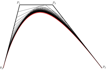
Figure 7: The sequence of polygons generated from 100 iterations of the corner cutting scheme (41) and (42) and parameters $n=3,r_{1}=2,r_{2}=4,r_{3}=14$ and $r_{j}=2j+10$ for $j\geq 4$. The red curve is the Gelfond-Bézier curve associated with the Müntz space $span(1,t^{2},t^{4},t^{1}4)$ and control polygon $(P_{0},P_{1},P_{2},P_{3})$

9 Shifted Gelfond-Bézier curves and curve design

As we have noted in remark 4, the Gelfond-Bernstein bases of Müntz spaces over an interval contained in $[0,1]$ and does not contain the origin coincide, in some sense, with the Chebyshev-Bernstein bases. Therefore, working with intervals that does not contain the origin has the drawback of loosing all the simplifications brought by the origin through the splitting principle of Schur functions. For curve design, in which for example we want to find conditions for the $C^{k}$ continuity between two Gelfond-Bézier curves, naturally one of the curves will be defined on an interval not containing the origin and then the $C^{k}$ continuity conditions will be relatively complex as was shown in [1]. One way to resolve this problem is to shift the origin to the left extremity of the interval in which each of the two curves are defined. This motivate the following definition.

Definition 7.

Let $\Lambda=(0=r_{0},r_{1},...,r_{n})$ be a sequence of strictly increasing real numbers and let $H^{n}_{k,\Lambda},k=0,...,n$ be the Gelfond-Bernstein basis associated with the Müntz space $E_{\Lambda}(n)$ over the interval $[0,1]$. We define the shifted Gelfond-Bernstein basis $\tilde{H}^{n}_{k,\Lambda},k=0,...,n$ over an interval $[a,b]$ by

$$\tilde{H}^{n}_{k,\Lambda}(t)=H^{n}_{k,\Lambda}(\frac{t-a}{b-a});\quad t\in[a,b]$$

Note that the shifted Gelfond-Bernstein basis $\tilde{H}^{n}_{k,\Lambda},k=0,...,n$ over an interval $[a,b]$ is not a basis of the Müntz space $E_{\Lambda}(n)$ but it is a basis of the shifted Müntz space $E_{\Lambda,a}(n)=span(1,(t-a)^{r_{1}},(t-a)^{r_{2}},...,(t-a)^{r_{n}})$. In the case the sequence $\Lambda=(0,1,...,n)$, then for any real number $a$, we have $E_{\Lambda}(n)=E_{\Lambda,a}(n)$, namely, the linear space of polynomials of degree $n$. In this case the shifted Gelfond-Bernstein basis over an interval $[a,b]$ coincide with the classical Bernstein basis over the interval $[a,b]$.

All the relevant properties of shifted Gelfond-Bernstein bases over an interval $[a,b]$ can be deduced by simple manipulations from the non-shifted ones. For example, let $\Lambda_{1}=(0=r_{0},r_{1},...,r_{n})$ and $\Lambda_{2}=(0=s_{0},s_{1},...,s_{n})$ be two sequences of strictly increasing real numbers and let $\tilde{H}^{n}_{k,\Lambda_{1}},k=0,...,n$ be the shifted Gelfond-Bernstein basis over an interval $[a,b]$ associated with the sequence $\Lambda_{1}$ and $\tilde{H}^{n}_{k,\Lambda_{2}},k=0,...,n$ be the shifted Gelfond-Bernstein basis over an interval $[b,c]$ associated with the sequence $\Lambda_{2}$. Consider now the following two shifted Gelfond-Bézier curves $\Gamma_{1}$ and $\Gamma_{2}$ with parameterizations

$$\begin{split}&\Gamma_{1}:\quad P(t)=\sum_{k=0}^{n}\tilde{H}_{k,\Lambda_{1}}^{n}(t)P_{k};\quad t\in[a,b]\\ &\Gamma_{2}:\quad Q(t)=\sum_{k=0}^{n}\tilde{H}_{k,\Lambda_{2}}^{n}(t)Q_{k};\quad t\in[b,c].\end{split}$$

For simplicity, we assume that the real number $s_{1}$ in the sequence $\Lambda_{2}$ is equal to one. Then, in this case, from Theorem 6, we have

$$P^{\prime}(b)=\frac{r_{n}}{b-a}\Delta P_{n-1}\quad\textnormal{and}\quad Q^{\prime}(c)=\frac{1}{c-b}\frac{\prod_{j=2}^{n}s_{j}}{\prod_{j=2}^{n}(s_{j}-1)}\Delta Q_{0}.$$

Therefore, a necessary and sufficient conditions for the two curves $\Gamma_{1}$ and $\Gamma_{2}$ to be $C^{1}$ at the point $P_{n}$ is that

$$P_{n}=Q_{0}\quad\textnormal{and}\quad\frac{r_{n}}{b-a}\Delta P_{n-1}=\frac{1}{c-b}\frac{\prod_{j=2}^{n}s_{j}}{\prod_{j=2}^{n}(s_{j}-1)}\Delta Q_{0}.$$

Figure 8, shows an example of $C_{1}$ continuity between two shifted Gelfond-Bézier curves of order $3$ associated respectively with the sequences $\Lambda_{1}=(0=r_{0},2,3,5)$ and $\Lambda_{2}=(0=s_{0},1,10,25)$ and defined respectively over the intervals $[1,2]$ and $[2,3]$. It is possible to study the conditions for the $C^{k},k\geq 2$ continuity and even define Gelfond splines. Such a study is still in progress and will be the subject of a forthcoming contribution.

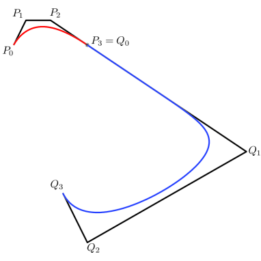
Figure 8: $C^{1}$ continuity at the point $P_{3}$ between two shifted Gelfond-Bézier curves associated with two different sequences. The shifted Gelfond-Bézier curve with control points $(P_{0},P_{1},P_{2},P_{3})$ is associated with the sequence $\Lambda_{1}=(0,2,3,5)$ and defined over the interval $[1,2]$, while the shifted Gelfond-Bézier curve with control points $(Q_{0},Q_{1},Q_{2},Q_{3})$ is associated with the sequence $\Lambda_{1}=(0,1,10,25)$ and defined over the interval $[1,2]$. (see text for more informations)

10 Conclusion

In this work, we carried out a comprehensive study of the generalized Bernstein bases in Müntz spaces defined by Hirschman, Widder and Gelfond and that we termed here as Gelfond-Bernstein bases. We revealed their connection with the Chebyshev-Bernstein bases in Müntz spaces, thereby legitimating their role as a possible fundamental tool in computer aided geometric design concepts. It it rather surprising that the Gelfond-Bernstein bases existed since 1949 and yet, to the best of our knowledge, they have never been incorporated into free form curve design utilities. We hope that this work will motivate further study of the applications of Gelfond-Bézier curves and surfaces as well as Gelfond splines to computer aided geometric design.

Acknowledgment : This work was partially supported by the MEXT Global COE project at Osaka University, Japan.

References

[1] R. Ait-Haddou, Y. Sakane and T. Nomura, Chebyshev blossom in Müntz spaces: toward shaping with Young diagrams. Submitted to Journal of Computational and
Applied Mathematics, ArXiv preprint arXiv:1107.2392, (2011).
[2] R. Ait-Haddou, Y. Sakane and T. Nomura,
A Müntz type theorem for a family of corner cutting schemes.
Submitted. ArXiv preprint arXiv:1111.3410v1, (2011).
[3] S. Bernstein, Démonstration du théoreme de Weierstrass
fondée sur le calcul des probabilités. Comm. Soc. Math. Kharkov 13, 1–2. (1912).
[4]P. Biane, L. Cantini and A. Sportiello, Doubly-refined
enumeration of alternating sign matrices and determinants of 2-staircase
Schur functions. ArXiv preprint arXiv:1101.3427v1, (2011).
[5] R. P. Boyer and L. C. Thiel, Generalized Berstein
polynomials and symmetric functions,
Advances in Applied Mathematics 28, 17- 39 (2002).
[6] A. O. Gelfond, On the generalized polynomials
of S. N. Bernstein (in russe) Izv. Akad. Nauk SSSR, ser. math.,
14, 413–420. (1950).
[7] I. I. Hirschman and D. V. Widder, Generalized
Bernstein polynomials. Duke Math. J., 16, 433–438. (1949).
[8] G. G. Lorentz, Bernstein polynomials. University
of Toronto Press, Toronto, (1953).
[9] I.G. Macdonald, Symmetric functions and Hall polynomials,
Oxford Math. Monographs, (1979).
[12] Ch. H. Müntz , Über den Approximationssatz von
Weierstrass, Mathematische Abhandlungen
in H. A. Schwarz’s Festschrift, Berlin, Springer, 303 -312. (1914).
[13] H. Pottmann, The geometry of Tchebycheffian splines, Comput.
Aided Geom. Design, 10, 181–210. (1993).
[14] H. Prautzsch and L. Kobbelt, Convergence of subdivision and degree elevation.
Advances in Computational Mathematics, 2, 143 -154 (1994).
[15] R. Winkel, Generalized Bernstein polynomials and Bézier curves:
An application of umbral calculus to computer aided geometric design, Advances
in Applied Mathematics 27, 51–81 (2001).