Automation of One-Loop Calculations with GoSam: Present Status and Future Outlook

Abstract

In this presentation, we describe the GoSam (Golem/Samurai) framework for the automated computation of multi-particle scattering amplitudes at the one-loop level. The amplitudes are generated analytically in terms of Feynman diagrams, and can be evaluated using either $D$-dimensional integrand reduction or tensor decomposition. GoSam can be used to compute one-loop corrections to Standard Model (QCD and EW) processes, and it is ready to link generic model files for theories Beyond SM. We show the main features of GoSam through its application to several examples of different complexity.

1 Introduction

The discovery potential of the experimental programs at the LHC relies heavily on the availability of higher order corrections for many relevant processes [1]. The searches for the Higgs boson and the compilation of related exclusion limits need precise calculations for Higgs’ signal and background processes. Further, it will be very important to have precise theory predictions at hand in order to constrain model parameters in the event that a signal of New Physics will be detected. Therefore, it is of major importance to provide tools for next-to-leading order (NLO) predictions which are largely automated such that signal and background rates for a multitude of processes can be estimated reliably.

Already some time ago, the idea of automating NLO calculations has been pursued with public programs like FeynArts [2] and QGRAF [3] for diagram generation and FormCalc/LoopTools [4] and GRACE [5] for the automated calculation of NLO corrections, primarily in the electroweak sector. In spite of this important progress, until the last few years we did not observe a large production of calculations of one-loop amplitudes involving more than four external legs. Only very recently, conceptual and technical advances in multi-leg one-loop calculations allowed the calculation of six-point [6, 7, 8, 9, 10, 11, 12, 13, 14, 15, 16, 17, 18, 19, 20, 21, 22] and even seven-point [23, 24] processes, and opened the door to the possibility of an automated generation and evaluation of multi-leg one-loop amplitudes, rather than creating a collection of hard-coded individual processes.

Even if excellent process-specific programs are available, like MCFM [25, 26, 27] and VBFNLO [28], nevertheless it is desirable to have flexible tools at hand such that, in the same fashion already available at the tree-level [29, 30, 31], any process which may turn out to be important can be promptly evaluated at NLO accuracy.

Recently, we observed major advances in the direction of constructing packages for fully automated one-loop calculations, see e.g. [32, 33, 34, 35, 36, 37, 38, 39, 40, 41]. Reviewing all the concepts that lead to these advances is beyond the scope of this presentation. In the development of our computational tools, the OPP reduction technique [43, 44] and generalized $D$-dimensional unitarity [45] turned out to be the most crucial ingredients.

The purpose of this talk is to present the program package GoSam [46] which allows the automated calculation of one-loop amplitudes for multi-particle processes. The integrand is generated via Feynman diagrams, using QGRAF [3], FORM [47], spinney [48] and haggies [49]. The individual program tasks are managed by python scripts. The only task required from the user is the preparation of an “input card” in order to launch the generation of the source code and its compilation, without having to worry about internal details of the code generation.

Concerning the reduction, the program offers the possibility to use either the $D$-dimensional extension of the OPP method, as implemented in SAMURAI [36], or tensor reduction as implemented in Golem95C [50, 51] interfaced through tensorial reconstruction at the integrand level [52], or a combination of both.

GoSam can be used to generate and evaluate one-loop corrections in both QCD and electro-weak theory. Beyond the Standard Model theories can be interfaced using FeynRules [53, 54] or LanHEP [55]. The Binoth-Les Houches-interface [56] to programs providing the real radiation contributions is also included.

In the following, we will provide a brief description of the main features of the code, with particular attention to the generation of the code and the various options to efficiently and automatically compute all rational terms. We will conclude the presentation with some examples of applications.

2 Main features of GoSam

GoSam produces in a fully automated way all the code required to perform the calculation of one-loop amplitudes, by processing the information contained in an “input card” prepared by the user. The main steps in this process are: the generation of contributing diagrams, the optimization and algebraic manipulation to simplify their expressions, and the writing of a FORTRAN code ready to be used within a phase-space integration. The reduction of unintegrated amplitudes to linear combinations of scalar (master) integrals is fully embedded in the process.

In this section, we give a brief overview of some general operations performed by GoSam. A complete description of the framework, together with a detailed explanation of all features available in GoSam, can be found in Ref. [46].

2.1 Diagram Generation

For the diagram generation both at tree level and one-loop level we employ the program QGRAF [3]. This program already offers several ways of excluding unwanted diagrams for example by requesting a certain number of propagators or vertices of a certain type or by specifying topological properties such as the presence of tadpoles or on-shell propagators. Although QGRAF is a very reliable and fast generator we added another filter over diagrams by means of Python. This gives several advantages: first of all, the possibilities offered by QGRAF are not always sufficient to distinguish certain classes of diagrams; secondly, QGRAF cannot handle the sign for diagrams with Majorana fermions in a reliable way; and finally, in order to fully optimize the reduction, we want to classify and group diagrams according to the sets of their propagators.

In our framework, QGRAF generates three sets of output files: an expression for each diagram for FORM [47], Python code for drawing each diagram and Python code for computing the properties of the diagram. The model information for QGRAF is either read from the built-in Standard Model file or is generated from a user defined LanHEP [55] or Universal FeynRules Output (UFO) [53] file. The Python program automatically performs several operations: diagrams whose color factor turns out to be zero are dropped; the number of propagators containing the loop momentum, the tensor rank and the kinematic invariants of the associated loop integral are computed; diagrams with a vanishing loop integral associated are detected and flagged for the diagram selection; all propagators and vertices are classified for the diagram selection; diagrams containing massive quark self-energy insertions or closed massless quark loops are specially flagged.

Partitioning diagrams with similar structures and tracking their rank are very important operations in order to reduce the number of operations performed by the reduction and allow allow for a big gain in efficiency: after carrying out the tensor reduction for one diagram, all other diagrams that contain only a subset of the denominators are reduced with virtually no additional computational cost. This is true both in the OPP method [43] as implemented in CutTools [32] and SAMURAI [36] and in classical tensor reduction methods as implemented in Golem95C [50, 51], PJFRY [57, 58] and LoopTools [4, 59].

During this phase, GoSam also generates a LaTeX file with the drawings of all contributing diagrams. To achieve this task, we use our own implementation of the algorithms described in Ref. [60] and Axodraw [61] to actually draw the diagrams.

2.2 Lorentz Algebra

Concerning the algebraic operations performed by GoSam to render the integral suitable for efficient numerical evaluation, one of the primary goals is to split the $(4-2\varepsilon)$ dimensional algebra into strictly four-dimensional objects and symbols representing the higher-dimensional remainder. In GoSam we have implemented the ’t Hooft-Veltman scheme (tHV) and dimensional reduction (DRED). In both schemes all external vectors (momenta and polarisation vectors) are kept in four dimensions. Internal vectors, however, are kept in the $n$-dimensional vector space. We adopt the conventions used in [48], where $\hat{k}$ denotes the four dimensional projection of an in general $n$ dimensional vector $k$. The $(n-4)$ dimensional orthogonal projection is denoted as $\tilde{k}$. For the integration momentum $q$ we introduce in addition the symbol $\mu^{2}=-\tilde{q}^{2}$, such that

$$q^{2}=\hat{q}^{2}+\tilde{q}^{2}=\hat{q}^{2}-\mu^{2}.$$ (1)

We also introduce suitable projectors by splitting the metric tensor

$$g^{\mu\nu}=\hat{g}^{\mu\nu}+\tilde{g}^{\mu\nu},\quad\hat{g}^{\mu\nu}\tilde{g}_{\nu\rho}=0,\quad\hat{g}^{\mu}_{\mu}=4,\quad\tilde{g}^{\mu}_{\mu}=n-4.$$ (2)

GoSam contains a library of representations of wave functions and propagators up to spin two. The exact form of the interaction vertices is taken from the model files.

Once all wave functions and propagators have been substituted by the above definitions and all vertices have been replaced by their corresponding expressions from the model file, all vector-like quantities and all metric tensors are split into their four-dimensional and their orthogonal part. As we use the ’t Hooft algebra, $\gamma_{5}$ is defined as a purely four-dimensional object, $\gamma_{5}=i\epsilon_{\mu\nu\rho\sigma}\hat{\gamma}^{\mu}\hat{\gamma}^{\nu}\hat{\gamma}^{\rho}\hat{\gamma}^{\sigma}$. By applying the usual anti-commutation relation for Dirac matrices we can separate the four-dimensional and $(n-4)$-dimensional parts of Dirac traces.

While the $(n-4)$-dimensional traces are reduced completely to products of $(n-4)$-dimensional metric tensors $\tilde{g}^{\mu\nu}$, the four-dimensional part is treated such that the number of terms in the resulting expression is kept as small as possible. Any spinor line or trace is broken up at any position where a light-like vector appears. Furthermore, Chisholm identities are used to resolve Lorentz contractions between both Dirac traces and open spinor lines. If any traces remain we use the built-in trace algorithm of FORM [47].

2.3 Treatment of $R_{2}$ terms

In the numerator of a one-loop diagram, terms containing the symbols $\mu^{2}$ or $\varepsilon$ can lead to a so-called $R_{2}$ term [62]. Therefore the numerator function can be written as,

$$\mathcal{N}(\hat{q},\mu^{2},\varepsilon)=\mathcal{N}_{0}(\hat{q},\mu^{2})+\varepsilon\mathcal{N}_{1}(\hat{q},\mu^{2})+\varepsilon^{2}\mathcal{N}_{2}(\hat{q},\mu^{2})\,.$$ (3)

It is useful to observe that the terms $\mathcal{N}_{1}$ and $\mathcal{N}_{2}$ in Eq. (3) do not arise in DRED, where only terms containing $\mu^{2}$ contribute to $R_{2}$. Instead of relying on the construction of $R_{2}$ from specialized Feynman rules [63, 64, 65, 66], we can generate the $R_{2}$ part along with all other contribution using automated algebraic manipulations.

The code offers the option between the implicit and explicit construction of the $R_{2}$ terms. The implicit construction uses the splitting of Eq. (3) and treats all numerator functions $\mathcal{N}_{i}$ on equal grounds. Each term in Eq. (3) is reduced separately and the results are added up taking into account the powers of $\varepsilon$. The explicit construction of $R_{2}$ is based on the fact that the non purely 4-dimensional part of the numerator function contains powers of $\mu^{2}$ or $\varepsilon$, and the expressions for the corresponding integrals are relatively simple and known explicitly. Therefore, after separating it using the algebraic manipulation described before, the $(n-4)$ dimensional part is computed analytically whereas the purely four-dimensional part is passed to the numerical reduction. This approach also allows for an efficient calculation of the $R_{2}$ alone.

2.4 Reduction to scalar (master) integrals

GoSam allows to choose at run-time (namely without regenerating the code) the preferred method of reduction. Available options include the integral-level $D$-dimensional reduction, as implemented in SAMURAI, or traditional tensor reduction as implemented in Golem95C interfaced through tensorial reconstruction at the integrand level, or a combination of both.

Concerning the scalar (tensorial) integrals [67, 68], GoSam allows to choose among a variety of options, including QCDLoop [69, 70], OneLoop [71], Golem95C [50, 51], plus the recently added PJFRY [57, 58] and LoopTools [4, 59]. Among these codes, OneLoop and Golem95C also fully support complex masses.

For details about the reduction methods, we refer the reader to previous presentations [37, 38, 39] or the original articles.

3 Examples

The GoSam codes have been tested on several processes, starting with QCD $2\to 2$ NLO amplitudes, but also on more challenging $2\to 4$ (not counting decays) in the final state. Some examples are depicted in Table 1. The full list of processes, with the details of all comparisons performed, is given in Ref. [46].

Process	Checked with Ref.
$u\overline{d}\to e^{-}\overline{\nu}_{e}\,g$	[40]
$e^{+}e^{-}\to e^{+}e^{-}\gamma$ (QED)	[72]
$pp\to H\,t\overline{t}$	[40]
$pp\to W^{+}W^{+}jj$	[20]
$pp\to b\overline{b}b\overline{b}$	[15, 16, 34]
$pp\to W^{+}W^{-}b\overline{b}$	[34, 40]
$u\overline{u}\to t\overline{t}b\overline{b}$	[34, 40]
$gg\to t\overline{t}b\overline{b}$	[34, 40]
$u\overline{d}\to W^{+}ggg$	[34]

Table 1: Some of the processes computed and checked with GoSam

3.1 BLHA interface, GoSam, and SHERPA

The BLHA interface allows to link GoSam to a general Monte Carlo event generator, which is responsible for supplying the missing ingredients for a complete NLO calculation of a physical cross section. Among those, SHERPA [73] offers the possibility to compute the LO cross section and the real corrections with both the subtraction terms and the corresponding integrated counterparts [74, 75, 76]. Using the BLHA interface, we linked GoSam with SHERPA to compute physical cross section for $W^{\pm}+1$-jet at NLO.

We tested our results producing distributions for inclusive and exclusive $p_{\perp}$ and $\eta$ of the jet, $H_{T}$, and for $p_{\perp}$ and $\eta$ of the leptons (details can be found in Ref. [46]). All distributions are in agreement with the ones produced using SHERPA in combination with MCFM.

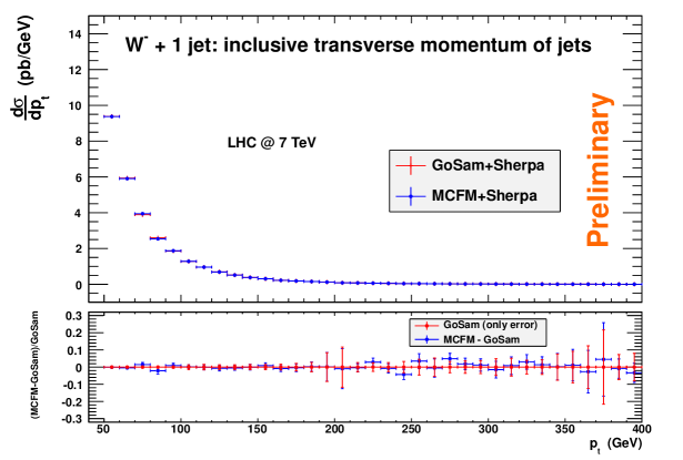
Figure 1: Comparison of the inclusive transverse momentum of $W^{-}+1$ jet between Sherpa interfaced with GoSam and Sherpa interfaced with MCFM. For comparison purpose we chose the $k_{T}$-algorithm with $p_{t,min}=50$ GeV. The bars indicate the statistical Monte Carlo error.

3.2 GoSam and Neutralino Pair Production

As an example of the usage of GoSam with a model file different from the Standard Model, we calculated the QCD corrections to neutralino pair production in the MSSM. A calculation of the total cross sections for neutralino pair production at the LHC is also presented in Ref. [77]. The model file has been imported via the UFO interface. To import such files within the GoSam setup, all the user has to do is to give the path to the corresponding model file in the input card.

In this example, we combined the one-loop amplitude with the real radiation corrections to obtain results for differential cross sections. For the infrared subtraction terms we employed MadDipole [78, 79], while the real emission part is calculated using MadGraph/MadEvent [80]. The virtual matrix element is renormalized in the $\overline{MS}$ scheme, while massive particles are treated in the on-shell scheme. The renormalization terms specific to the massive MSSM particles have been added manually. For the SUSY parameters we use the modified benchmarks point SPS1amod suggested in [81], and use $\sqrt{s}=7$ TeV.

In Fig.2 we show the differential cross section for the $m_{\chi_{1}^{0}\chi_{1}^{0}}$ invariant mass, where we employed a jet veto to suppress large contributions from the channel $qg\rightarrow\chi_{1}^{0}\chi_{1}^{0}q$ which opens up at order $\alpha^{2}\alpha_{s}$, but for large $p_{T}^{jet}$ belongs to the distinct process of neutralino pair plus one hard jet production at leading order.

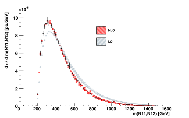
Figure 2: Comparison of the NLO and LO $m_{\chi_{1}^{0}\chi_{1}^{0}}$ distributions for the process $pp\rightarrow\chi_{1}^{0}\chi_{1}^{0}$ with a jet veto on jets with $p^{jet}_{T}>20$ GeV and $\eta<4.5$. The band gives the dependence of the result on $\mu=\mu_{F}=\mu_{R}$ between $\mu_{0}/2$ and $2\mu_{0}$. We choose $\mu_{0}=m_{Z}$. The black line gives the bin error for the value at the central scale.

4 Outlook and Conclusions

In the last five years, we observed major advances in our understanding of one-loop scattering amplitudes. Aside from improvement on standard tensorial techniques, the development of unitarity-based approaches, paired with the decomposition at the integrand level contained in OPP method, changed the landscape of this field, favoring the calculation of NLO amplitudes for several challenging processes and the development of new theoretical frameworks and tools for such calculations.

For quite a long time, tree-level calculation have been fully automated and included in flexible multi-process tools [29, 30]. The level of automation achieved by one-loop calculations is suggesting the possibility of a similar success also for the NLO. One of the natural hopes for the future is to devise ways of extending and generalizing what we understood so far about one-loop amplitudes, in order to develop tools and methods for higher-order calculations [82, 83, 84], but plenty of work is still needed to achieve this goal.

In this presentation, we illustrated the main features of GoSam, a new program package for the fully automated evaluation of one-loop scattering amplitudes in any renormalizable quantum field theory. In its present form, GoSam can be used to calculate one-loop corrections both in QCD and electro-weak theory and offers the flexibility to link general model files for theories Beyond the Standard Model. The amplitudes are generated in terms of Feynman diagrams and the reduction to master (scalar) integrals can be performed in several ways, which can be selected at run-time.

We presented several examples of one-loop calculations performed within the GoSam framework, as well as preliminary results of interesting applications such as the interface with SHERPA. These examples demonstrate the great flexibility, together with a competitive timing, of GoSam. We are looking forward to tackle more challenging calculations and interfacing with other existing tools in the coming months.

Acknowledgments
G.C. and G.L. are supported by the British Science and Technology Facilities Council (STFC). N.G. was supported in part by the U.S. Department of Energy under contract No. DE-FG02-91ER40677. P.M. and T.R. were supported by the Alexander von Humboldt Foundation, in the framework of the Sofja Kovaleskaja Award Project “Advanced Mathematical Methods for Particle Physics”, endowed by the German Federal Ministry of Education and Research. The work of G.O. was supported in part by the National Science Foundation under Grant PHY-0855489 and PSC-CUNY Award #63275-00 41. The research of F.T. is supported by Marie-Curie-IEF, project: ”SAMURAI-Apps”.

References

-
[1]
Z. Bern et al. arXiv:0803.0494 [hep-ph];
J. R. Andersen et al. arXiv:1003.1241 [hep-ph]. - [2] T. Hahn, Comput. Phys. Commun. 140 (2001) 418-431.
- [3] P. Nogueira, J. Comput. Phys. 105 (1993) 279–289.
- [4] T. Hahn, M. Perez-Victoria, Comput. Phys. Commun. 118 (1999) 153-165.
- [5] G. Belanger et al., Phys. Rept. 430 (2006) 117-209.
- [6] C. F. Berger et al., Phys. Rev. D80 (2009) 074036.
- [7] C. F. Berger et al., Phys. Rev. Lett. 102 (2009) 222001.
- [8] R. K. Ellis, K. Melnikov, G. Zanderighi, Phys. Rev. D80 (2009) 094002.
- [9] K. Melnikov, G. Zanderighi, Phys. Rev. D81 (2010) 074025.
- [10] C. F. Berger et al., Phys. Rev. D82 (2010) 074002.
- [11] A. Bredenstein et al., Phys. Rev. Lett. 103 (2009) 012002.
- [12] A. Bredenstein et al., JHEP 1003 (2010) 021.
- [13] G. Bevilacqua et al., JHEP 0909 (2009) 109.
- [14] G. Bevilacqua et al., Phys. Rev. Lett. 104 (2010) 162002.
- [15] T. Binoth et al., Phys. Lett. B685 (2010) 293-296.
- [16] N. Greiner et al., Phys. Rev. Lett. 107 (2011) 102002.
- [17] G. Bevilacqua et al., JHEP 1102 (2011) 083.
- [18] G. Bevilacqua et al., [arXiv:1108.2851 [hep-ph]].
- [19] A. Denner et al., Phys. Rev. Lett. 106 (2011) 052001.
- [20] T. Melia et al., JHEP 1012 (2010) 053.
- [21] T. Melia et al., Phys. Rev. D83 (2011) 114043.
- [22] F. Campanario et al., Phys. Lett. B704 (2011) 515-519.
- [23] C. F. Berger et al., Phys. Rev. Lett. 106 (2011) 092001.
- [24] H. Ita et al., [arXiv:1108.2229 [hep-ph]].
- [25] J. M. Campbell, R. K. Ellis, Phys. Rev. D60 (1999) 113006.
- [26] J. M. Campbell, R. K. Ellis, Phys. Rev. D62 (2000) 114012.
- [27] J. M. Campbell, R. K. Ellis, C. Williams, JHEP 1107 (2011) 018.
- [28] K. Arnold et al., [arXiv:1107.4038 [hep-ph]].
- [29] A. Kanaki and C. G. Papadopoulos, Comput. Phys. Commun. 132 (2000) 306; A. Cafarella, C. G. Papadopoulos and M. Worek, Comput. Phys. Commun. 180, 1941 (2009).
- [30] T. Stelzer and W. F. Long, Comput. Phys. Commun. 81 (1994) 357.
- [31] J. Alwall et al., JHEP 1106 (2011) 128.
- [32] G. Ossola, C. G. Papadopoulos, R. Pittau, JHEP 0803 (2008) 042.
- [33] P. Mastrolia et al., JHEP 0806 (2008) 030.
- [34] A. van Hameren, C. G. Papadopoulos, R. Pittau, JHEP 0909 (2009) 106.
- [35] G. Bevilacqua et al., Nucl. Phys. Proc. Suppl. 205-206 (2010) 211-217.
- [36] P. Mastrolia et al., JHEP 1008 (2010) 080.
- [37] G. Ossola, PoS ACAT2010 (2010) 075.
- [38] G. Cullen et al., Nucl. Phys. Proc. Suppl. 205-206 (2010) 67-73.
- [39] T. Reiter et al., [arXiv:1011.6632 [hep-ph]].
- [40] V. Hirschi et al., JHEP 1105 (2011) 044.
- [41] G. Bevilacqua et al., [arXiv:1110.1499 [hep-ph]].
- [42] M. Czakon, these proceedings; A. van Hameren, these proceedings; D. Kosower, these proceedings; M. Worek, these proceedings.
- [43] G. Ossola, C. G. Papadopoulos, R. Pittau, Nucl. Phys. B763 (2007) 147-169.
- [44] G. Ossola, C. G. Papadopoulos, R. Pittau, JHEP 0707 (2007) 085.
- [45] R. K. Ellis et al., Nucl. Phys. B822 (2009) 270-282.
- [46] G. Cullen et al., arXiv:1111.2034 [hep-ph].
- [47] J. A. M. Vermaseren, arXiv:math-ph/0010025.
- [48] G. Cullen, M. Koch-Janusz, T. Reiter, Comput. Phys. Commun. 182 (2011) 2368-2387.
- [49] T. Reiter, Comput. Phys. Commun. 181, 1301 (2010).
- [50] T. Binoth et al., Comput. Phys. Commun. 180 (2009) 2317-2330.
- [51] G. Cullen et al., Comput. Phys. Commun. 182 (2011) 2276-2284.
- [52] G. Heinrich et al., JHEP 1010 (2010) 105.
- [53] C. Degrande et al., [arXiv:1108.2040 [hep-ph]].
- [54] N. D. Christensen, C. Duhr, Comput. Phys. Commun. 180 (2009) 1614-1641.
- [55] A. Semenov, [arXiv:1005.1909 [hep-ph]].
- [56] T. Binoth et al., Comput. Phys. Commun. 181 (2010) 1612-1622.
- [57] J. Fleischer, T. Riemann, Phys. Rev. D83 (2011) 073004.
- [58] V. Yundin, these proceedings.
- [59] G. J. van Oldenborgh, J. A. M. Vermaseren, Z. Phys. C46 (1990) 425-438.
- [60] T. Ohl, Comput. Phys. Commun. 90 (1995) 340-354.
- [61] J. A. M. Vermaseren, Comput. Phys. Commun. 83 (1994) 45-58.
- [62] G. Ossola, C. G. Papadopoulos, R. Pittau, JHEP 0805 (2008) 004.
- [63] P. Draggiotis et al., JHEP 0904 (2009) 072.
- [64] M. V. Garzelli, I. Malamos, R. Pittau, JHEP 1001 (2010) 040.
- [65] M. V. Garzelli, I. Malamos, R. Pittau, JHEP 1101 (2011) 029.
- [66] M. V. Garzelli, I. Malamos, Eur. Phys. J. C71 (2011) 1605.
- [67] G. ’t Hooft and M. J. G. Veltman, Nucl. Phys. B 153 (1979) 365.
- [68] G. Passarino and M. J. G. Veltman, Nucl. Phys. B 160 (1979) 151.
- [69] R. K. Ellis, G. Zanderighi, JHEP 0802 (2008) 002.
- [70] G. J. van Oldenborgh, Comput. Phys. Commun. 66 (1991) 1-15.
- [71] A. van Hameren, Comput. Phys. Commun. 182 (2011) 2427-2438.
-
[72]
S. Actis, P. Mastrolia, G. Ossola,
Phys. Lett. B682 (2010) 419-427;
S. Actis, P. Mastrolia, G. Ossola, Acta Phys. Polon. B40 (2009) 2957-2963. - [73] T. Gleisberg et al., JHEP 0902 (2009) 007.
- [74] F. Krauss, R. Kuhn, G. Soff, JHEP 0202 (2002) 044.
- [75] T. Gleisberg, F. Krauss, Eur. Phys. J. C53 (2008) 501-523.
- [76] M. Schonherr, F. Krauss, JHEP 0812 (2008) 018.
- [77] W. Beenakker et al., Phys. Rev. Lett. 83 (1999) 3780-3783.
- [78] R. Frederix, T. Gehrmann, N. Greiner, JHEP 0809 (2008) 122.
- [79] R. Frederix, T. Gehrmann, N. Greiner, JHEP 1006 (2010) 086.
- [80] J. Alwall et al., JHEP 0709 (2007) 028.
- [81] B. Feigl, H. Rzehak, D. Zeppenfeld, [arXiv:1108.1110 [hep-ph]].
- [82] J. Gluza, K. Kajda, D. A. Kosower, Phys. Rev. D83 (2011) 045012.
- [83] P. Mastrolia, G. Ossola, [arXiv:1107.6041 [hep-ph]].
- [84] D. A. Kosower, K. J. Larsen, [arXiv:1108.1180 [hep-th]].