On Searching for Small Kochen-Specker
Vector Systems (extended version)

Abstract

Kochen-Specker (KS) vector systems are sets of vectors in $\mathbb{R}^{3}$ with the property that it is impossible to assign 0s and 1s to the vectors in such a way that no two orthogonal vectors are assigned 0 and no three mutually orthogonal vectors are assigned 1. The existence of such sets forms the basis of the Kochen-Specker and Free Will theorems. Currently, the smallest known KS vector system contains 31 vectors. In this paper, we establish a lower bound of 18 on the size of any KS vector system. This requires us to consider a mix of graph-theoretic and topological embedding problems, which we investigate both from theoretical and practical angles. We propose several algorithms to tackle these problems and report on extensive experiments. At the time of writing, a large gap remains between the best lower and upper bounds for the minimum size of KS vector systems.

Keywords: Kochen-Specker vector systems; topological graph embedding problems; constraint solving; graph enumeration algorithms.

1 Introduction

In a recent, thought-provoking paper, John H. Conway and Simon Kochen demonstrate that “if […] there exist any experimenters with a modicum of free will, then elementary particles must have their own share of this valuable commodity” [11]. More precisely, Conway and Kochen consider so-called ‘spin-1’ particles (such as photons) whose ‘spin’ (a physical property) can be measured along any given direction. The squared outcome of such measurements is always either 0 or 1. Conway and Kochen’s Free Will theorem asserts that, if an experimenter can choose the direction along which to perform a spin-1 experiment freely (i.e., in a way that is not determined by the past), then the response of the spin-1 particle to such an experiment is also not determined by the past.

This theorem rests on three basic axioms of quantum mechanics and relativity, the most crucial of which (for our purposes) is the following:

The SPIN Axiom [11]. Measurements of the squared components of spin of a spin-1 particle in three orthogonal directions always yield the outcomes 1, 0, 1 in some order.

The SPIN axiom not only follows from the postulates of quantum mechanics, but has also been verified experimentally [13]. This axiom alone already gives rise to what is known as the ‘Kochen-Specker paradox’ [12]: if the response of a spin-1 particle to any conceivable spin measurement were predetermined prior to the actual measurement, then those responses would define a function from the unit sphere in three dimensions to the set $\{0,1\}$, satisfying the so-called 101-property: any three points on the sphere with mutually orthogonal position vectors must be assigned the values 1, 0, 1 in some order. The Kochen-Specker paradox—which is in fact a mathematical theorem—is that no such function exists.

The impossibility of such ‘101-functions’ can be proved by exhibiting a finite set of points on the sphere on which such functions cannot be defined. The first such set, discovered by Kochen and Specker more than forty years ago, contained 117 points [15]. Subsequent sets, usually referred to as ‘records’ [21], cut this number down to 33 and then 31 [24]. The latter is the size of the smallest known ‘Kochen-Specker vector system’, discovered approximately 20 years ago by Conway and Kochen.

As pointed out in [21], finding small Kochen-Specker vector systems has both theoretical and practical motivations. Conway himself has stressed the problem on several occasions whilst giving public lectures on the Free Will theorem. The work we describe here reports on some partial progress in this endeavour; our main result is that any Kochen-Specker vector systems must contain at least 18 vectors (Thm. 4.4). Achieving this bound required us to consider a mix of graph-theoretic and topological embedding problems, for which we devised and analysed a number of algorithms. In addition, we establish bounds on the theoretical complexity of some of the principal problems involved (Thms. 2.1 and 3.1), and also show that the key task of checking canonicity in the 30-year-old Colbourn-Read orderly graph enumeration algorithm [10] cannot belong to NP—and much less to P—unless NP = co-NP (Thm. 4.1).

Unfortunately, it would appear that narrowing the gap between the best lower and upper bounds for the minimum size of KS vector systems remains a formidable challenge, and significant progress in this area will likely require substantially new ideas.

The work most closely related to ours is that of Pavičić et al. [22, 21]. They consider higher-dimensional generalisations of the problem treated in this paper, but their formulation and results are incomparable to ours. We return to the differences between our approach and theirs in Sec. 2; we also refer the reader to [22, 1] for a more thorough discussion of the matter.

Different Standards of Proof. Due to the mixed discrete/continuous aspects of the problems considered in this paper, it is important to pay special attention to the nature of the proofs involved. The usual kind of proof is mathematical. Along with such proofs, we also present several results that have computer-aided proofs, in which extensive calculations were carried out by computer. A third category of results could be deemed to have numerical proofs, by which we mean that a computer program was used and floating-point arithmetic was involved in a way that cannot be guaranteed to be entirely accurate. It is reasonable to assume that the results thus obtained are very likely to be correct, but it remains conceivable that a highly ill-conditioned initial problem could lead to an incorrect answer.

It should be stressed that in this paper, we do not consider numerical calculations and proofs to be sufficiently reliable to be fully adequate; however, we have frequently made use of numerical techniques as heuristics in order to guide and accelerate the search for computer-aided proofs of our main results. The latter should be viewed as having the same strength as traditional pencil-and-paper, mathematical proofs.

2 Kochen-Specker Vector Systems

Kochen-Specker vector systems can be represented in multiple ways. In the Introduction, we have implicitly described such systems as certain finite sets of points on the surface of the sphere $\mathbb{S}^{2}$. In fact, an immediate consequence of the SPIN axiom is that squared-spin measurements along opposite directions necessarily yield the same outcome, so that it is sensible to identify antipodal points. Accordingly, let us therefore define a vector system as a finite subset of the open northern hemisphere $\mathbb{H}^{2}=\{(x,y,z):x^{2}+y^{2}+z^{2}=1\mathrm{\ and\ }z>0\}$. Alternatively, vector systems can be represented as finite subsets of the projective plane $\mathbb{P}^{2}$, and also as finite sets of points on the surface of a cube, where once again we identify antipodal points. We variously make use of all three of these representations in the rest of this paper.

A vector system $\mathcal{K}\subseteq\mathbb{H}^{2}$ is said to be 101-colourable if it is possible to assign either 0 or 1 to each vector in $\mathcal{K}$ such that (i) no two orthogonal vectors are both assigned 0, and (ii) no three mutually orthogonal vectors are all assigned 1.

Finally, a Kochen-Specker (KS) vector system is a vector system that is not 101-colourable. The size of such a system is simply the number of vectors it contains.

At the time of writing, the smallest known KS vector system is still the one discovered approximately twenty years ago by Conway and Kochen [24]. The 31 vectors of this system can be represented as lying on a cubic grid centered at the origin, as depicted in Fig. 1. Note that orthogonality relationships among the vectors are easily inferred through elementary geometry, thanks to the regularity of the grid. Non-101-colourability can be established by (somewhat tedious) case analysis.

Figure 1: A visual representation of Conway and Kochen’s KS vector system of size 31.

Note that the colourability conditions (i) and (ii) as given above, although in appearance stronger than the SPIN axiom, are implicitly equivalent to it. For instance, while the SPIN axiom, strictly speaking, asserts nothing about a vector system consisting of exactly two orthogonal vectors, it implicitly requires one of these vectors to be assigned 1, since if both were assigned 0 one could derive a contradiction by considering a third vector orthogonal to the other two.

This seemingly innocuous observation has consequences for the way in which KS vector systems are built and measured. Pavičić et al. [21] and Larsson [16], for example, require every pair of orthogonal vectors to belong to a triple of mutually orthogonal vectors, invoking a strict application of the SPIN axiom. Following this convention, they argue that the KS vector system depicted in Fig. 1 should be viewed as having size 51 rather than 31 (cf. [21]): indeed, this system as represented above contains 20 pairs of orthogonal vectors without a third orthogonal vector present.

In contrast, our own conventions—following, among others, [15, 23, 24, 7, 11, 12]—are predicated on colourability conditions (i) and (ii) as given earlier. For further discussion on the matter, we refer the reader to [21] and [1].

Vector Systems and Graphs. Any vector system $\mathcal{K}$ gives rise to an associated undirected graph $G_{\mathcal{K}}$, the vertices of which are the vectors of $\mathcal{K}$, with an edge between two vertices iff the corresponding vectors are orthogonal. In other words, $G_{\mathcal{K}}=(V,E)$, where $V=\mathcal{K}$ and $E=\{\{\vec{u},\vec{v}\}:\vec{u},\vec{v}\in\mathcal{K}\mathrm{\ and\ }\vec{u}\cdot\vec{v}=0\}$.

We define 101-colourability for graphs in the obvious way: assignment of 0 or 1 to the vertices in such a way that (i) no two adjacent vertices are both assigned 0, and (ii) no triangle (3-clique) is assigned all 1s. Clearly, $\mathcal{K}$ is a KS vector system iff $G_{\mathcal{K}}$ is not 101-colourable.

Of course, an arbitrary graph $H$ may not correspond to any realisable (3-dimensional) vector system: the orthogonality constraints corresponding to graph edges may fail to be simultaneously satisfiable. Let us define a graph $H$ to be embeddable if there exists some vector system that it corresponds to. More precisely, we ask that there be a vector system $\mathcal{K}$ that can be put in one-to-one correspondence with the vertices of $H$ in such a way that adjacent vertices are mapped to orthogonal vectors. Note that we do not require that non-adjacent vertices should go to non-orthogonal vectors; this relaxation simplifies the embeddability-checking process, discussed in Sec. 3. However, it is necessary for distinct vertices to go to distinct vectors. Formally, $H=(V,E)$ is embeddable if it has a supergraph $H^{\prime}=(V,E^{\prime})$ over the same set of vertices such that $H^{\prime}$ is isomorphic to $G_{\mathcal{K}}$ for some vector system $\mathcal{K}$.

Finding a small KS vector system therefore corresponds to finding a small graph that is both not 101-colourable and embeddable, and accordingly this is the approach we have followed and report on in this paper.

Note that any graph containing a square (4-cycle) is unembeddable: indeed, orthogonality constraints would force a pair of opposite vertices of the square to be mapped to collinear (i.e., identical) vectors. Accordingly, we shall mainly focus on square-free graphs in the remainder of this paper. This turns out to be a fairly powerful restriction: all square-free graphs with 9 or fewer vertices are embeddable, while there are only two distinct (up to isomorphism) unembeddable square-free graphs with 10 vertices [1].

A second interesting observation about embeddable graphs is the following:

Proposition 1

Any embeddable graph is 4-colourable.

To see this, consider an embeddable graph $G$ and let $\mathcal{K}$ be an embedding of it as a vector system in the hemisphere $\mathbb{H}^{2}$. Partition $\mathbb{H}^{2}$ into four quadrants as delineated by the $xz$-plane and the $yz$-plane, and colour each vector of $\mathcal{K}$ according to the quadrant it lies in. Since vectors belonging to the same quadrant cannot be mutually orthogonal, corresponding vertices of $G$ cannot be adjacent. Thus the quadrant colouring of $\mathcal{K}$ gives rise to a valid 4-colouring of $G$. ∎

As the next result indicates, 101-colourability is in theory an expensive condition to check, even when restricting to graphs that are both square-free and 4-colourable. In practice, however, our SAT-based colourability checker (implemented using MiniSat 2.0 [19]) was systematically able to decide 101-colourability of graphs having at most 30 vertices in microseconds. In fact, experiments with graphs having hundreds of vertices also completed well within a millisecond.

Theorem 2.1

Deciding whether a square-free 4-colourable graph is 101-colourable is NP-complete.

Membership in NP is obvious, whereas hardness can be shown by reduction from 3-colourability of an arbitrary graph $G$: replace every vertex of $G$ by a triangle (which can be 101-coloured in precisely three ways) and replace each edge of $G$ by a gadget ensuring that the corresponding ‘adjacent’ triangles are coloured differently. This can be done whilst ensuring that the resulting graph is both square-free and 4-colourable—details can be found in [1]. ∎

Finally, note that every 3-colourable graph is automatically 101-colourable.

3 Embeddability

In this section, we examine the problem of determining whether a given (square-free) graph is embeddable or not.

It is fairly straightforward to see that embeddability queries can be phrased in the existential theory of the reals: given a graph $G$, postulate a triple of real variables $(x,y,z)$ for every vertex of $G$, and express the various constraints using polynomial equalities and inequalities. For example, $x^{2}+y^{2}+z^{2}=1$ and $z>0$ together ensure that the corresponding vector should lie in the hemisphere $\mathbb{H}^{2}$. Orthogonality constraints are likewise expressed by setting the relevant dot products equal to zero, and so on. Embeddability of the graph $G$ therefore corresponds to solvability of this constraint system over the reals.

It is plain that the constraints can be constructed in polynomial time. Since the existential theory of the reals has polynomial space complexity [9, 28], we have:

Theorem 3.1

Graph embeddability can be decided in PSPACE.

For a graph with 30 vertices, the corresponding constraint system requires 90 real variables (or rather, assuming the graph has at least one triangle, 81 variables since we can quotient out rotational symmetries by fixing the vectors associated with one of its triangles). Unfortunately, current real arithmetic solvers cannot in practice handle systems containing more than just a handful of real variables. Thm. 3.1 is therefore mainly of theoretical interest at the present time.

Our next observation is that, given a graph $G$, one can in fact construct a single multivariate polynomial $P_{G}$ over the reals such that $G$ is embeddable iff $P_{G}$ has a root. We simply extend the above approach by transforming inequalities into equalities, through the use of auxiliary variables, and conjoining multiple equalities into a single one via a standard squaring trick. For example, the inequality $z>0$ is equivalent to the conjunction of the equalities $uv=1$ and $u^{2}=z$, where $u$ and $v$ are implicitly existentially quantified. In turn, both equalities can be conjoined into a single one by writing $(uv-1)^{2}+(u^{2}-z)^{2}=0$, etc. We therefore have:

Proposition 2

A graph $G$ is embeddable iff the polynomial $P_{G}$ has a real root.

It is easy to see that we can arrange for $P_{G}$ to have degree four. Moreover, graphs with at most 30 vertices give rise to polynomials in fewer than 1000 variables (the bulk of which are required to ensure that all vectors are pairwise distinct). Unfortunately, deciding whether such polynomials have real roots is in general also well beyond the practical capabilities of today’s algorithms and computers. For an in-depth account of relevant algorithms and results in this area, we refer the reader to [4].

Finally, let us remark that graph embeddability can alternatively be phrased in terms of isometric (i.e., distance-preserving) embeddability: a graph is embeddable (in the sense of this paper) iff its vertices can distinctly be placed in the upper half of $\mathbb{R}^{3}$ so as to lie at distance 1 from the origin, and such that adjacent vertices are precisely $\sqrt{2}$ units apart. More information on isometric embeddings and related topics in topological graph theory can be found in [5].

Homotopy Continuation. Homotopy continuation is a rigorous yet fairly practical approach to solving systems of polynomial equations over the reals. We experimented extensively with Bertini [6], a state-of-the-art software package for numerical algebraic geometry. We briefly describe below some of the algorithms underlying Bertini; for an authoritative and thorough treatment we refer the reader to [30].

The general idea of homotopy continuation is the following: Given a system of polynomial equations $\{f_{i}({\overline{x}})=0\}$ in variables $\overline{x}$ that we are trying to solve (the ‘target’ system), find another system of equations $\{g_{i}(\overline{x})=0\}$ with known solutions and of matching degrees (the ‘start’ system). Consider the system of equations $\{h_{i}(\overline{x},t)=tg_{i}(\overline{x})+(1-t)f_{i}(\overline{x})=0\}$. We know the solution of $\{h_{i}(\overline{x},t)=0\}$ at $t=1$ and are seeking a solution at $t=0$. Assuming that ‘nothing goes wrong’ (which is a strong assumption, see [30] for details), we can numerically track the paths of the roots of $\{h_{i}(\overline{x},t)\}$ as $t$ goes from $1$ to $0$. This can be done, for example, by using Euler prediction and Newton correction steps.

In order for this process to be successful, it is necessary to work over complex rather than real numbers. When combined with several enhancements, such as the gamma trick, which makes use of a random number generator in order to avoid bad start systems with high probability, the method finds all the isolated roots of the target system $\{f\}$, with a probability that can be made arbitrarily high. If $\{f\}$ has only isolated roots and the number of these equals the number of roots of $\{g\}$, then the method not only finds numerical approximations to all the roots of $\{f\}$, but also in doing so, demonstrates that there are no non-isolated roots. To get a match in the number of roots of $\{f\}$ and $\{g\}$, it can be helpful to consider multi-degree structures [30]. At the conclusion of the continuation, it is then necessary to check which of the roots thus obtained are indeed real.

Note that orthogonality constraints are homogeneous. Since Bertini allows the definition of homogeneous groups of variables, it is possible to work directly in the complex projective plane $\mathbb{CP}^{2}$ and soundly dispense with all inequalities as well as the equations requiring vectors to have unit length.

In order for a constraint system to have isolated solutions, it is necessary to quotient out rotational symmetries, for example by fixing three mutually orthogonal vectors. We must then have precisely as many equations as unknowns.

Any embedding found by Bertini should be considered a numerical existence proof, due to the use of floating-point numbers. Of course, such solutions are however a very strong indication that a genuine embedding does exist, which can then potentially be confirmed by more expensive but exact methods. Moreover, under certain conditions, if Bertini asserts that the solution set is empty then this should also be considered a numerical proof (of unembeddability), valid with high probability.

In our experiments, Bertini was found to be relatively efficient on small systems of equations. Unfortunately, its performance quickly degraded with larger systems. For example, it was unable to solve (a subset of) the constraints arising from the Conway-Kochen vector system given in Fig. 1 within a week’s running time.

Interval Arithmetic. Interval arithmetic is a well-known methodology for performing mathematically reliable numerical computations. It is used by Pavičić et al. in [22, 21] to tackle very similar embeddability problems to the ones we consider here. Comprehensive treatments of the subject can be found in a number of excellent texts such as [20].

The basic idea underlying interval arithmetic is to replace precise valuations of the variables with intervals in which a solution, if it exists, must lie. Interval manipulations are performed by operations on interval bounds that can even take into account rounding errors due to floating-point arithmetic.

A collection of intervals, one for each variable appearing in a system of equations, is called a box. Various techniques can be used to progressively decrease the size of boxes, zeroing in on a solution. When this process is exhausted, boxes are split into smaller sub-boxes (a technique known as ‘bisection’) and each case is analysed separately.

Under the right circumstances, interval arithmetic can provide a genuine, computer-aided proof—and not merely a numerical proof—that a given graph is unembeddable: this requires covering the entire space of potential solutions with a finite number of (possibly very small) boxes, for each of which the system of equations provably has no solution. Conversely, an interval arithmetic solver can also produce computer-aided proofs of embeddability by proving that a root must lie in a given box. This can be achieved through several means, the most well-known of which employs an analogue of Newton’s method for intervals. Of course, interval arithmetic can also produce numerical proofs of both embeddability and unembeddability by narrowing in sufficiently closely on particular regions of the state space.

Our implementation of an interval arithmetic solver made heavy use of routines from the PROFIL library [25]. Its performance varied greatly, but it was able to produce proofs of both existence and absence of embeddings for many of the graphs we experimented with. Among others, it found a valid embedding for the graph underlying the 31-vector Conway-Kochen system in a matter of seconds.

As explained in [1], graphs that have a large number of different 3-colourings will automatically possess a large number of degenerate solutions (in which distinct vertices are mapped to collinear vectors). Such solutions are especially difficult for an interval analyser to handle, as they require a large number of correct bisection decisions to be made and moreover produce a huge number of boxes. Fortunately, as noted earlier, 3-colourable graphs are ipso facto 101-colourable, and are therefore not candidates for producing KS vector systems in the first place. Since 101-colourability is in practice dramatically easier to establish than unembeddability, this potential drawback is largely circumvented in practice.

Cubic Grids. Conway and Kochen’s KS vector system of size 31 lies on a regular cubic grid, as shown in Fig. 1. That grid can be viewed as consisting of all vectors with integer coordinates lying on the surface of the cube $[-2,2]^{3}$, with antipodal points identified.

We can, of course, consider grids of different granularities by introducing a grid parameter $N$: the corresponding grid can be viewed as the set of vectors with integer coordinates lying on the surface of the cube $[-N,N]^{3}$, again with antipodal points identified.

One of the chief advantages of cubic grids is that all orthogonality relationships are inferable by straightforward inspection; thus grid embeddability provides a genuine mathematical proof of embeddability. Moreover, we have so far not encountered any graph which we believed to be embeddable (through the use of homotopy continuation or interval arithmetic) yet which was not found to be embeddable on some cubic grid. This leads us to formulate the following:

Conjecture 1

Every embeddable graph can be embedded on some cubic grid.

Note that a graph is embeddable on some cubic grid iff it has an embedding on the surface of the unit cube $[-1,1]^{3}$ using only rational coordinates. Interestingly, an assertion analogous to Conjecture 1 concerning the hemisphere $\mathbb{H}^{2}$ turns out to be false: as shown in [18], the set of rational vectors on $\mathbb{H}^{2}$ (which is dense) can be 101-coloured. Thus no KS vector system can possibly be represented on $\mathbb{H}^{2}$ using exclusively rational coordinates.

In our experiments, we found grid-solving to be consistently highly efficient. For example, embedding the 31-vertex Conway-Kochen graph took less than 10ms on the grid with parameter $N=2$, approximately 250ms on the $(N\mbox{$=$}8)$-grid, and 26s on the $(N\mbox{$=$}12)$-grid. Naturally, all embeddability proofs carry mathematical certainty; however the absence of a grid embedding does not allow one to draw any conclusion regarding (proper) embeddability.

Let us conclude this section by noting that embeddability clearly remains a highly challenging problem at present, and seemingly one of the hardest obstacles to obtaining tighter results than we have been able to achieve to date.

4 Lower Bounds

A natural strategy for finding small KS vector systems is first to search for small graphs that are not 101-colourable. Such graphs should moreover be square-free (otherwise they cannot be embeddable) and connected (otherwise a smaller instance would be available).

Our initial approach was to generate these graphs at random, subject to various parameters, and check whether they are embeddable. Several hundred millions of connected square-free graphs were generated, yielding thousands that were not 101-colourable. Unfortunately, for most graphs with 30 vertices or less, we were simply unable to determine embeddability; and the ones for which we did succeed were all found to be unembeddable. Interestingly, our random graph generator produced several isomorphic copies of the 31-vertex Conway-Kochen specimen.

We then turned to sub-systems of the various cubic grids, which are embeddable by construction. We were able to exhaustively search the grids with parameters $N=2$ and $N=4$; all vector systems of size 30 or less were found to be 101-colourable, whereas the only systems of size 31 that were not 101-colourable were all isomorphic to the 31-vector Conway-Kochen system. We also randomly sampled extensively from sub-systems of the grids with parameters $N=6$, $N=8$, and $N=12$. Again, no smaller system was found, and all KS systems of size 31 were found to be isomorphic to the Conway-Kochen system.

Enumerating Connected Square-Free Graphs. At the time of writing, the On-Line Encyclopedia of Integer Sequences [29] lists the numbers of non-isomorphic connected square-free graphs with up to and including 17 vertices: there are 19,297,850,417 in total, and 17,992,683,043 on 17 vertices alone. We re-enumerated all these graphs and checked each one for 101-colourability, a task which required solving more than 19 billion instances of an NP-complete problem.

In [10], Colbourn and Read propose an ‘orderly’ procedure for graph enumeration. The key idea is to generate the adjacency matrices of graphs in unique canonical forms. More precisely, given an adjacency matrix, consider the bit-string obtained by concatenating the entries strictly above the diagonal, column by column (from top to bottom), left to right. The canonical representation of a given graph $G$ is the unique adjacency matrix of $G$ with the greatest bit-string value in lexicographic order.

As pointed out in [10], a crucial property of this particular notion of canonicity is the following: if $\mathbf{M}$ is the canonical adjacency matrix of a graph $G$ on $n$ vertices, then the $(n-1)\times(n-1)$ submatrix of $\mathbf{M}$ obtained by deleting the last column and the last row of $\mathbf{M}$ is also the canonical adjacency matrix of some subgraph of $G$ on $n-1$ vertices. In the terminology of [26] (see also [17]), this enables the design of an effective graph enumeration algorithm: Generate the adjacency matrices of graphs on a fixed number of vertices by a depth-first search process which starts from the trivial $1\times 1$ matrix and successively augments the matrix by adding a single column and row to it until the target number of vertices has been reached. In so doing, whenever a non-canonical matrix is encountered, immediately discard it and backtrack. This procedure guarantees that every canonical matrix will appear exactly once at some point in the search. Moreover, the number of non-canonical matrices that are produced (and immediately discarded) in the process is kept relatively low.

A second key advantage of the Colbourn-Read notion of canonicity is that one may use it to enumerate all non-isomorphic graphs with some hereditary property (i.e., any property of a graph which automatically holds for all its induced subgraphs). Note however that while square-freeness is clearly hereditary, connectedness is not. Nevertheless, the following result shows that the Colbourn-Read algorithm is still suitable for our purposes:

Proposition 3

Suppose that $\mathbf{M}$ is the canonical adjacency matrix of a connected graph $G$. Then the submatrix of $\mathbf{M}$ obtained by deleting the last column and the last row of $\mathbf{M}$ is also the (canonical) adjacency matrix of some connected subgraph of $G$.

To see this, consider a graph $H$ over $n$ vertices having at least two components, with canonical matrix $\mathbf{M}$. We claim that all the vertices of one of its components will appear first in $\mathbf{M}$. For clarity, let us list the vertices of $H$ as $1,2,\ldots,n$ in the order in which they appear in $\mathbf{M}$. Let $A$ be the component of $H$ which contains vertex $1$, and let $i$ be the smallest vertex that does not belong to $A$. Suppose, for a contradiction, that vertex $j<i$ is connected to some vertex greater than $i$, which we will call $k$. Note that all $i-1$ entries of the $i^{\mathrm{th}}$ column above the diagonal are 0. However, the $j^{\mathrm{th}}$ entry of the $k^{\mathrm{th}}$ column is 1 (since $j$ is connected to $k$) and therefore by swapping vertices $i$ and $k$ (which would not affect any of the entries above the diagonal to the left of $i$) one would obtain an adjacency matrix for (a graph isomorphic to) $H$ with strictly greater bit-string value than $\mathbf{M}$, contradicting the canonicity of $\mathbf{M}$.

We now show that the last vertex (call it $n$) in the canonical representation $\mathbf{M}$ of a connected graph $G$ is not a cut vertex. Indeed, if removing $n$ disconnects $G$, then $G-\{n\}$ has at least two components, and moreover there is an edge in $G$ from $n$ to each of the components of $G-\{n\}$. Recall however that the submatrix of $\mathbf{M}$ obtained by deleting the last column and row of $\mathbf{M}$ is a canonical representation of $G-\{n\}$. Therefore all the vertices of some component $A$ of $G-\{n\}$ appear first in $\mathbf{M}$. Moreover the first vertex $i$ not belonging to $A$ has all entries above the diagonal set to 0. Lastly, since $n$ is connected in $G$ to some vertex $j<i$, swapping vertices $i$ and $n$ would yield an adjacency matrix for $G$ with strictly greater bit-string value than $\mathbf{M}$, contradicting the canonicity of $\mathbf{M}$. This concludes the proof of Prop. 3.∎

A major attraction of orderly graph enumeration algorithms is that “expensive isomorphism tests are replaced by relatively inexpensive verifications of canonicity” [10]—see also [26, 27, 17]. Canonicity checking is indeed a pivotal component of the Colbourn-Read algorithm, yet somewhat surprisingly its precise complexity appears to have remained open since orderly algorithms were first introduced 30 years ago. We provide some partial answers to this question below.

The first observation is that canonicity checking is clearly in co-NP: if a matrix is not canonical, then one needs only exhibit another one that is higher in lexicographic order together with an isomorphism between the two. We now establish a hardness result:

Theorem 4.1

If the problem of canonicity checking were in NP, then NP =co-NP.

We show that an NP algorithm for canonicity checking would entail the existence of an NP algorithm for proving that a graph has no clique of size a given integer $k$. Since the latter is well-known to be co-NP-complete, the conclusion that NP = co-NP would follow.

Note that the canonical adjacency matrix of a graph having a clique of size $k$ will necessarily contain 1s in the upper-left triangle covering vertices up to $k$, for otherwise an adjacency matrix with a higher lexicographic order could immediately be obtained by re-labelling the vertices of the clique with the integers 1 to $k$. Conversely, any adjacency matrix with an upper-left triangle covering vertices up to $k$ consisting entirely of 1s necessarily represents a graph having a clique of size $k$.

Let $G$ be a graph that has no clique of size $k$. Guess the canonical adjacency matrix for $G$, guess and verify the adjacency mapping showing that the matrix does indeed represent $G$, and verify that the matrix is indeed canonical using the putative NP algorithm for canonicity checking. By the above observation, the upper-left triangle of this matrix covering vertices up to $k$ cannot consist entirely of 1s, thereby proving that all cliques in $G$ must have size strictly less than $k$. ∎

Thm. 4.1 strongly suggests that canonicity checking is unlikely to be in NP, and much less in P.

Note however that this hardness result is not obviously applicable to square-free graphs, since in particular the latter have no cliques of size greater than 3. We are nonetheless able to establish the following weaker statement:

Theorem 4.2

If the problem of canonicity checking for adjacency matrices of square-free graphs were in NP, then the graph isomorphism problem (for arbitrary graphs) would be in co-NP.

To prove Thm. 4.2, one first notices that the graph isomorphism problem for square-free graphs is polynomial-time equivalent to the graph isomorphism problem for arbitrary graphs: given arbitrary graphs $G$ and $H$, transform both into square-free graphs $G^{\prime}$ and $H^{\prime}$ by subdividing every edge exactly once. Then $G$ and $H$ are isomorphic iff $G^{\prime}$ and $H^{\prime}$ are isomorphic.

Suppose now that there were an NP algorithm for checking canonicity of adjacency matrices of square-free graphs. Given two non-isomorphic graphs $G$ and $H$, one could produce a certificate of non-isomorphism by exhibiting the canonical adjacency matrices of $G^{\prime}$ and $H^{\prime}$ (as defined above), together with the mappings showing that these matrices are indeed adjacency representations of $G^{\prime}$ and $H^{\prime}$ respectively. Finally, validate that these matrices are indeed canonical using the putative NP algorithm, and verify by inspection that the two matrices differ. This proves that $G$ and $H$ are not isomorphic and concludes the proof of Thm. 4.2. ∎

We conjecture that both canonicity checking and canonicity checking for square-free graphs are in fact co-NP-complete. Note that the related but considerably more general problem of determining whether a string is lexicographically maximum amongst all strings in its orbit under a given arbitrary permutation group of the letters’ positions is known to be co-NP-complete [14]. However it does not seem possible to import that paper’s techniques to our setting since the corresponding permutation group acting on the set of entries of an adjacency matrix is induced by the full permutation group on the labellings of the vertices of the graph and as such is highly constrained.

In practice, notwithstanding Thms. 4.1 and 4.2, we have found that canonicity checking could be made extremely efficient. We implemented a fairly simple backtracking algorithm which enabled us to check canonicity of the vast majority of matrices with 17 vertices or fewer within microseconds. This led us to the following computer-aided result:

Theorem 4.3

Every square-free graph with at most 16 vertices is 101-colourable. Moreover, there is a unique graph with 17 vertices that is not 101-colourable (shown on the left-hand side of Fig. 2).

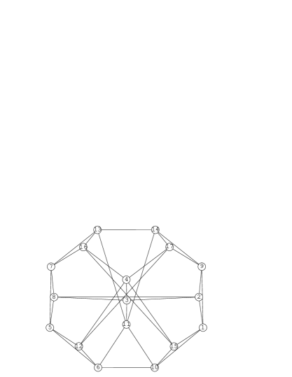
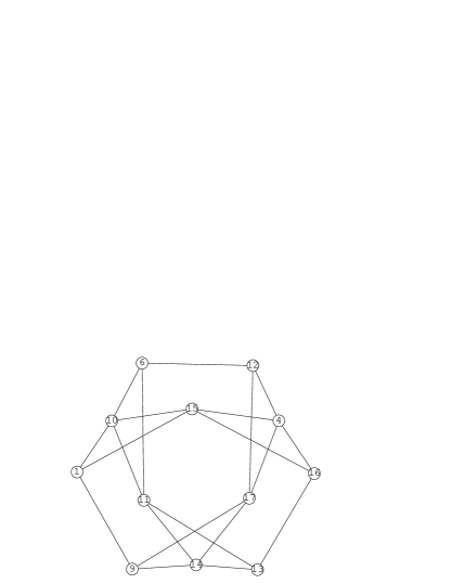
Figure 2: The unique square-free graph on 17 vertices that is not 101-colourable (left), together with its smallest unembeddable subgraph.

Our next task was naturally to determine whether this 17-vertex candidate is actually embeddable. Unfortunately, the answer is no. Using Bertini, we identified a 12-vertex subgraph (shown on the right-hand side of Fig. 2) whose associated embedding polynomial was shown to have precisely 12 distinct complex roots, none of which are purely real. This produces a numerical proof of the fact that our 17-vertex candidate cannot be embedded. Finally, we were able to upgrade this to a computer-aided proof using our interval arithmetic solver, yielding the following lower bound:

Theorem 4.4

A Kochen-Specker vector system must contain at least 18 vectors.

Unfortunately, Thm. 4.4 still leaves an astronomical gap to bridge before proving that Conway and Kochen’s KS vector system of size 31 is the smallest possible (if indeed that is the case). Extrapolating from known data, the graph below suggests that there are some $10^{32}$ connected square-free graphs on 30 vertices or less, well out of the brute-force reach of current technology.

5 Conclusion

We have proposed the problem of finding small Kochen-Specker vector systems—or proving that none exist of size less than 31—as a difficult and worthwhile algorithmic challenge. Higher-dimensional generalisations of the problem have also been considered by others, notably Pavičić et al. [21].

The results we have obtained (greater details of which are available in [1]) can largely be summarised by listing a number of properties that any minimal KS vector system must enjoy. Such a system:

• has at most 31 vectors (Conway and Kochen’s KS vector system);

• contains at least 18 vectors (Thm. 4.4);

• has associated graph that is square-free (Sec. 2);

• has associated graph that is not 101-colourable and not 3-colourable (Sec. 2);

• has associated graph that is 4-colourable (Prop. 1);

• has associated graph with minimum degree 3 [1];

• has associated graph in which each vertex belongs to a triangle [1];

• is not a subsystem of the cubic grid with grid parameter $N=4$, unless it is the Conway-Kochen 31-vector system itself (Sec. 3).

In our view, two central challenges are to (i) devise more efficient algorithms for determining graph embeddability (in which respect Conjecture 1 could play a key role), and (ii) find efficient means to drastically cut down the number of candidate graphs that must be examined.

Acknowledgements. We thank Nick Trefethen for introducing the first two authors to the third, Jean-Pierre Merlet for sharing his experience on interval arithmetic, and Don Knuth for drawing our attention to [10]. Following publication of the short version of this paper [2], Adán Cabello informed us that the unique square-free uncolourable graph on 17 vertices depicted in Fig. 2 had already been discovered by John Smolin several years earlier. To the best of our knowledge, this graph was never published, nor were the methods used to obtain it disclosed. Cabello further claims in [8] to have proof that this graph is unembeddable, although the reference he gives in op. cit. is again unpublished.

The second author was supported by EPSRC and the third author was supported by NSF grant DMS-0712910.

References

-
[1]
F. Arends.
A lower bound on the size of the smallest Kochen-Specker vector
system.
Master’s thesis, Oxford University, 2009.
www.cs.ox.ac.uk/people/joel.ouaknine/download/arends09.pdf. - [2] F. Arends, J. Ouaknine, and C. W. Wampler. On searching for small Kochen-Specker vector systems. In Proc. WG, volume 6986 of Springer LNCS, 2011.
- [3] L. Babai and E. M. Luks. Canonical labeling of graphs. In Proc. STOC. ACM, 1983.
- [4] S. Basu, R. Pollack, and M.-F. Roy. Algorithms in Real Algebraic Geometry. Springer, 2006.
- [5] L. W. Beineke and R. J. Wilson, editors. Topics in Topological Graph Theory, Encyclopedia of Mathematics and its Applications. Cambridge University Press, 2009.
- [6] www.nd.edu/sommese/bertini/.
- [7] J. Bub. Schütte’s tautology and the Kochen-Specker theorem. Found. Phys., 26:787–806, 1996.
- [8] A. Cabello. How many questions do you need to prove that unasked questions have no answers? Int. J. Quant. Info., 4(1):55–61, 2006.
- [9] J. Canny. Some algebraic and geometric computations in PSPACE. In Proc. STOC. ACM, 1988.
- [10] C. J. Colbourn and R. C. Read. Orderly algorithms for graph generation. Int. J. Comput. Math., 7:167–172, 1979.
- [11] J. H. Conway and S. Kochen. The free will theorem. Found. Phys., 36(10):1441–1473, 2006.
- [12] J. H. Conway and S. Kochen. The strong free will theorem. Notices of the AMS, 56(2), 2009.
- [13] Y.-F. Huang, C.-F. Li, Y.-S. Zhang, J.-W. Pan, and G.-C. Guo. Experimental test of the Kochen-Specker theorem with single photons. Phys. Rev. Lett., 90(250401), 2003.
- [14] T. A. Junttila. A note on the computational complexity of a string orbit problem (draft). Unpublished, 2001.
- [15] S. Kochen and E. P. Specker. The problem of hidden variables in quantum mechanics. J. Math. Mech., 17:235–263, 1967.
- [16] J.-Å. Larsson. A Kochen-Specker inequality. Europhys. Lett., 58:799–805, 2002.
- [17] B. D. McKay. Isomorph-free exhaustive generation. J. Alg., 26:306–324, 1998.
- [18] D. Meyer. Finite precision measurement nullifies the Kochen-Specker theorem. Phys. Rev. Lett., 83:3751–3754, 1999.
- [19] www.minisat.se/.
- [20] R. E. Moore, R. B. Kearfott, and M. J. Cloud. Introduction to Interval Analysis. SIAM, 2009.
- [21] M. Pavičić, J.-P. Merlet, B. McKay, and N. D. Megill. Kochen-Specker vectors. J. Phys. A: Math. Gen., 38(7):1577–1592, 2005.
- [22] M. Pavičić, J.-P. Merlet, and N. D. Megill. Exhaustive enumeration of Kochen-Specker vector systems. Research report RR-5388, INRIA, 2004.
- [23] A. Peres. Two simple proofs of the Kochen-Specker theorem. J. Phys. A: Math. Gen., 24:L175–L178, 1991.
- [24] A. Peres. Quantum Theory: Concepts and Methods. Kluwer, 1993.
- [25] www.ti3.tu-harburg.de/.
- [26] R. C. Read. Every one a winner, or: How to avoid isomorphism search when cataloguing combinatorial configurations. Annals Discrete Math., 2:107–120, 1978.
- [27] R. C. Read. A survey of graph generation techniques. In Lecture Notes in Mathematics, volume 884. Springer, 1981.
- [28] J. Renegar. On the computational complexity and geometry of the first-order theory of the reals. Parts I-III. J. Symb. Comput., 13(3):255–352, 1992.
-
[29]
N. J. A. Sloane.
The On-Line Encyclopedia of Integer Sequences, 2010.
www.research.att.com/njas/sequences/. - [30] A. J. Sommese and C. W. Wampler. The Numerical Solution to Systems of Polynomials Arising in Engineering and Science. World Scientific, 2005.