Rigorous Performance Bounds for Quadratic and Nested Dynamical Decoupling

Abstract

We present rigorous performance bounds for the quadratic dynamical decoupling (QDD) pulse sequence which protects a qubit from general decoherence, and for its nested generalization to an arbitrary number of qubits. Our bounds apply under the assumption of instantaneous pulses and of bounded perturbing environment and qubit-environment Hamiltonians such as those realized by baths of nuclear spins in quantum dots. We prove that if the total sequence time is fixed then the trace-norm distance between the unperturbed and protected system states can be made arbitrarily small by increasing the number of applied pulses.

I Introduction

The coupling between a quantum system and its environment typically causes decoherence, which is detrimental in quantum information processing (QIP) as it results in computational errors Nielsen and Chuang (2000). Over the years, various ways of suppressing quantum decoherence have been explored; see, e.g., Ref. M. S. Byrd and D. A. Lidar (2003). The methodology we study here is dynamical decoupling (DD), which utilizes sequences of strong pulses to decouple the system from its environment Viola and Lloyd (1998); Ban (1998); Zanardi (1999); Viola et al. (1999); Byrd and Lidar (2001). Recently, an optimal DD pulse sequence was discovered for the suppression of pure dephasing or longitudinal relaxation of a qubit coupled to a bath with a hard high frequency cutoff: Uhrig DD (UDD) Uhrig (2007); B. Lee (2008); Uhrig (2008); Yang and Liu (2008); Biercuk et al. (2009, 2009). In UDD, the instants $t_{j}$ ($j\in\{1,2\ldots N\}$) at which $N$ instantaneous $\pi$ pulses are applied are given by $t_{j}=T\lambda_{j}$, where $T$ is the total time of the sequence, and

$$\lambda_{j}=\sin^{2}\frac{j\pi}{2N+2}.$$ (1)

By optimal it is meant that each additional pulse suppresses dephasing or longitudinal relaxation to one additional order in an expansion in powers of $T$, i.e., $N$ pulses reduce dephasing or longitudinal relaxation to $\mathcal{O}(T^{N+1})$. Rigorous performance bounds were established in Ref. Uhrig and Lidar (2010). In this work we derive performance bounds for more general pulse sequences.

A near-optimal way to suppress general single-qubit decoherence, as opposed to only pure dephasing or pure longitudinal relaxation, is the quadratic DD (QDD) sequence West et al. (2010); Wang and Liu (2011); Quiroz and Lidar (2011); Kuo and Lidar (2011); Jiang and Imambekov (2011). A QDD sequence is obtained by nesting two UDD sequences of pulses which are orthogonal in spin space. When these two UDD sequences comprise the same number of pulses, $N$, a QDD sequence of $(N+1)^{2}$ pulses will suppress general qubit decoherence to $\mathcal{O}(T^{N+1})$, which is known from brute-force symbolic algebra solutions for small $N$ to be near-optimal West et al. (2010). It has been analytically proven that when the two UDD sequences comprise different numbers of pulses, $N_{1}$ and $N_{2}$, a QDD sequence of $(N_{1}+1)(N_{2}+1)$ pulses will suppress general qubit decoherence to $\mathcal{O}(T^{\min(N_{1},N_{2})+1})$, and this is universal, i.e., holds for arbitrary baths and system-bath interactions Wang and Liu (2011); Kuo and Lidar (2011); Jiang and Imambekov (2011). Moreover, the dependence of the suppression order of each single qubit error type (dephasing, bit flip, or both) on $N_{1}$ and $N_{2}$ has also been established in detail both in terms of analytical bounds Kuo and Lidar (2011) and numerical simulations Quiroz and Lidar (2011); Pasini and Uhrig (2011).

When the nesting process of UDD sequences is continued, one has the nested UDD (NUDD) sequence, which can protect multiple qubits, or general multi-level quantum systems, against general decoherence Wang and Liu (2011); Jiang and Imambekov (2011). It has been proven that NUDD is universal, and will suppress general multi-qubit decoherence to $\mathcal{O}(T^{\min_{i}(N_{i})+1})$, where $N_{i}$ are the orders of the UDD sequences being nested Jiang and Imambekov (2011). However, it is known that NUDD is sub-optimal Wang and Liu (2011).

Our main results in this paper are analytical upper bounds, for QDD and NUDD, on the trace-norm distance between the states of the DD-protected qubit or qubits, and the unperturbed qubit or qubits, given as a function of the total evolution time and the norms of the bath operators. Under the assumption that the bath operators have finite norms, the upper bound for NUDD shows that the trace-norm distance can be made arbitrarily small as a function of the minimal decoupling order $N$ of the UDD sequences comprising the NUDD sequence. In the QDD case, a tighter bound is obtained by having different decoupling orders for different types of decoherence errors, using the results of Ref. Kuo and Lidar (2011).

The structure of this paper is as follows. We develop our results for QDD and NUDD in parallel, always starting with the simpler case of QDD. We first review the QDD and NUDD sequences in Section II. We also derive bounding series for the two sequences in this section. In Section III we use the bounding series in order to find explicit upper bounds on the different single-axis errors for QDD, and similar explicit upper bounds on different error types for NUDD. These results are then used in Section IV to derive the main results of this paper: trace-norm distance upper bounds for QDD and NUDD. We conclude in Section V, and present additional technical details in the Appendix.

II Model

In this section we give a formal description of the QDD and NUDD sequences, and the decoherence they suppress.

II.1 QDD

We describe QDD as a nesting of two UDD sequences. The inner UDD sequence, denoted UDD${}_{N_{1}}$, comprises $N_{1}$ $Z$-type pulses, meaning $N_{1}$ instantaneous rotations by $\pi$ about the $z$-axis of the qubit Bloch sphere, i.e., $Z=ie^{-i(\pi/2)\sigma_{z}}$. Similarly, the outer UDD sequence, denoted UDD${}_{N_{2}}$, comprises $N_{2}$ $X$-type pulses, where $X=ie^{-i(\pi/2)\sigma_{x}}$. We denote the resulting QDD sequence by QDD${}_{N_{1},N_{2}}$. To make sure that the qubit state is unaltered by the sequence itself, we append an additional pulse at the conclusion of the sequence if $N_{1}$ or $N_{2}$ is odd. Thus, if $N^{\prime}_{i}$, denotes the number of pulses in UDD${}_{N_{i}}$, where $i\in\{1,2\}$, then

$$N^{\prime}_{i}=N_{i}+N_{i}\mbox{ mod }2.$$ (2)

We define the dimensionless relative time $s:=t/T$, so that the $X$-type pulses are applied at times

$$\lambda_{j}=\sin^{2}\frac{j\pi}{2N_{2}+2}$$ (3)

where $j=1,2,\ldots,N^{\prime}_{2}$ and the $Z$-type pulses are applied at times

$$\lambda_{j,k}=\lambda_{j-1}+(\lambda_{j}-\lambda_{j-1})\sin^{2}\frac{k\pi}{2N_{1}+2}$$ (4)

where $k=1,2,\ldots,N^{\prime}_{1}$.

We consider the most general form of “bounded” time-independent single-qubit decoherence, which is described by the Hamiltonian

$$\widetilde{H}=\sum_{\alpha\in\{0,x,y,z\}}\sigma_{\alpha}\otimes B_{\alpha}$$ (5)

where $\sigma_{0}=\mathbb{1}_{\text{S}}$ is the identity operator on the system. The operators $B_{\alpha}$ with $\alpha\in\{0,x,y,z\}$ are arbitrary except for the requirement that their sup-operator norms, i.e., the largest eigenvalue of $(B_{\alpha}^{\dagger}B_{\alpha})^{1/2}$, are finite

$$J_{\alpha}:=\|B_{\alpha}\|<\infty.$$ (6)

To decouple the qubit from the bath, we apply the QDD${}_{N_{1},N_{2}}\mbox{ }$sequence, assuming Eq. (5). See Fig. 1 for a schematic depiction of a QDD_3,3 sequence.

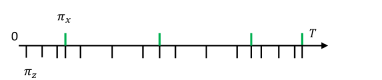
Figure 1: (Color online) Illustration of QDD_3,3. Time flows from left to right. The switching instants are distributed according to Eqs. (3) and (4). The pulses $\pi_{z}$ and $\pi_{x}$ are rotations about the $z$ and $x$ axes, respectively, by the angle $\pi$. The total sequence time is $T$.

The QDD${}_{N_{1},N_{2}}\mbox{ }$sequence is generated by the control Hamiltonian

$$H_{c}(s)=\frac{\pi}{2}{\sigma_{x}}\sum_{j=1}^{N^{\prime}_{2}}\delta(s-\lambda_{j})+\frac{\pi}{2}{\sigma_{z}}\sum_{j=1}^{N_{2}+1}\sum_{k=1}^{N^{\prime}_{1}}\delta(s-\lambda_{j,k}).$$ (7)

The corresponding control time-evolution operator is

$$U_{c}(s)={\cal T}\exp\left(-i\int_{0}^{s}H_{c}(s^{\prime})ds^{\prime}\right),$$ (8)

where $\cal T$ is the time-ordering operator. Thus, the toggling-frame Hamiltonian reads

$$H(s) = U^{\dagger}_{c}(s){\widetilde{H}}U_{c}(s)$$ (9a)

$$= \sum_{\alpha\in\{0,x,y,z\}}f_{\alpha}(s)\sigma_{\alpha}\otimes B_{\alpha},$$ (9b)

where the switching functions are

$$f_{0}{(s)} = 1\hskip 75.3998pt{s\in}[0,1],$$ (10a)

$$f_{x}(s) = (-1)^{k-1}\hskip 44.95535pt{s\in}[\lambda_{j,k-1},\lambda_{j,k}),$$ (10b)

$$f_{y}(s) = (-1)^{k-1}(-1)^{j-1}\hskip 9.95845pt{s\in}[\lambda_{j,k-1},\lambda_{j,k}),$$ (10c)

$$f_{z}(s) = (-1)^{j-1}\hskip 45.5244pt{s\in}[\lambda_{j-1},\lambda_{j}).$$ (10d)

For later use, we note that

$$f_{y}(s)=f_{x}(s)f_{z}(s).$$ (11)

Next, we consider the total time evolution given by the unitary operator

$$U(T)={\cal T}\exp\big{(}-iT\int_{0}^{1}H(s)ds\big{)}.$$ (12)

Standard time dependent perturbation theory provides the following Dyson series for $U(T)$

$$U(T) = \sum_{n=0}^{\infty}(-iT)^{n}\sum_{\{\vec{\alpha};\mathrm{dim}(\vec{\alpha})=n\}}f_{\vec{\alpha}}\widehat{Q}_{\vec{\alpha}}$$ (13a)

$$f_{\vec{\alpha}} := \int_{0}^{1}ds_{n}f_{\alpha_{n}}(s_{n})\int_{0}^{s_{n}}ds_{n-1}f_{\alpha_{n-1}}(s_{n-1})\ldots$$ (13b)

$$\int_{0}^{s_{3}}ds_{2}f_{\alpha_{2}}(s_{2})\int_{0}^{s_{2}}ds_{1}f_{\alpha_{1}}(s_{1})$$

$$\widehat{Q}_{\vec{\alpha}} := (\sigma_{\alpha_{n}}\otimes B_{\alpha_{n}})\cdots(\sigma_{\alpha_{1}}\otimes B_{\alpha_{1}})$$ (13c)

$$= r\sigma_{0}^{n_{0}}\sigma_{x}^{n_{x}}\sigma_{y}^{n_{y}}\sigma_{z}^{n_{z}}\otimes B_{\alpha_{n}}\cdots B_{\alpha_{1}}.$$ (13d)

The notation $\mathrm{dim}(\vec{\alpha})=n$ in Eq. (13a) means that the vector $\vec{\alpha}$ is restricted to having $n$ component $\{\alpha_{n},\dots,\alpha_{1}\}$. The components are $\alpha_{k}\in\{0,x,y,z\}$ for $1\leq k\leq n$. Each integer $n_{\alpha}\geq 0,\alpha\in\{0,x,y,z\}$ counts how many times the operator $\sigma_{\alpha}\otimes B_{\alpha}$ appears in $\widehat{Q}_{\vec{\alpha}}$. For given dimension $n$ of $\vec{\alpha}$, we have $n=n_{0}+n_{x}+n_{y}+n_{z}$. In this way, the complete sum over all possible sequences of $B_{0}$, $B_{x}$, $B_{y}$, and $B_{z}$ are considered. The rearrangement of the non-commuting product of Pauli matrices in Eq. (13c) into the canonical form (13d) gives rise to $r=(-1)^{v}$ where $v$ counts the number of times two different Pauli-matrices have to pass each other based on $\sigma_{\alpha}\sigma_{\beta}=-\sigma_{\beta}\sigma_{\alpha}$ if $\alpha\neq\beta$.

Our goal is to find an upper bound for each term $f_{\vec{\alpha}}\widehat{Q}_{\vec{\alpha}}$ separately. We exploit $|f_{\alpha}(s)|=1$, $\|\sigma_{\alpha}\|=1$, and

$$\|\widehat{Q}_{\vec{\alpha}}\| \leq J_{\vec{\alpha}}$$ (14a)

$$J_{\vec{\alpha}} := J_{\alpha_{n}}J_{\alpha_{n-1}}\ldots J_{\alpha_{1}}$$ (14b)

to obtain the upper bounding series given below for the series (13a) term by term

$$\|U(T)\| \leq \sum_{n=0}^{\infty}T^{n}F_{n}\sum_{\{\vec{\alpha};\mathrm{dim}(\vec{\alpha})=n\}}J_{\vec{\alpha}}$$ (15a)

$$=: S_{\text{Q}}(T)$$ (15b)

$$= \exp[(J_{0}+J_{x}+J_{y}+J_{z})T],$$ (15c)

where

$$F_{n}:=\int_{0}^{1}ds_{n}\int_{0}^{s_{n}}ds_{n-1}\ldots\int_{0}^{s_{3}}ds_{2}\int_{0}^{s_{2}}ds_{1}=\frac{1}{n!}.$$ (16)

The equality between (15a) and (15c) is most easily seen by realizing that the right hand side of (15a) is the Dyson series of (15c) as obtained by time dependent perturbation theory. This series will be used extensively when we compute the performance bounds in Section III which generalize the UDD results in Ref. Uhrig and Lidar (2010).

II.2 NUDD

The NUDD sequence is a generalization of the UDD and QDD sequences that suppresses decoherence for a multi-qubit system. Assume that the system comprises $m$ qubits. We consider the most general form of “bounded” time-independent $m$-qubit decoherence. Subject only to the constraint on the bath operators $B_{\vec{\mu}}$ that they are bounded

$$J_{\vec{\mu}}:=\|B_{\vec{\mu}}\|{<\infty},$$ (17)

the Hamiltonian that gives rise to this general decoherence is

$$\widetilde{H}=\sum_{\vec{\mu}\in{D_{m}}}\widehat{\sigma}_{\vec{\mu}}\otimes B_{\vec{\mu}}$$ (18)

where

$${D_{m}} {:=} {\{(0,0),(1,0),(1,1),(0,1)\}^{m}}$$ (19a)

$$\widehat{\sigma}_{\vec{\mu}} := \sigma_{1,\mu_{1}}\otimes\cdots\otimes\sigma_{m,\mu_{m}}.$$ (19b)

Here the $\sigma_{j,\mu_{j}}$’s are Pauli matrices or the identity and we use $j\in\{1,\dots,m\}$ to index the qubits. For the $j$th qubit, we use the binary component ${\mu_{j}}\in\{(0,0),(1,0),(1,1),(0,1)\}$ of the vector $\vec{\mu}:=(\mu_{1},\mu_{2},\ldots,\mu_{m})$ to denote the Pauli matrix subscripts $\{0,x,y,z\}$, respectively.

The NUDD sequence for an $m$-qubit system consists of $2m$ nested levels (two per qubit). Let $T$ be the total duration of the NUDD sequence and $N^{\prime}_{i}$ be the decoupling order of the $i$th-level UDD [Eq. (2)]. Then the pulses at the $i$th level are applied at the instants

$$\lambda_{l_{2m},l_{2m-1},...,l_{i}}$$ (20)

$$= \lambda_{l_{2m},l_{2m-1},...,l_{i+1}}+(\lambda_{l_{2m},l_{2m-1},...,l_{i+1}+1}$$

$${}-\lambda_{l_{2m},l_{2m-1},...,l_{i+1}})\sin^{2}\frac{l_{i}\pi}{2N^{\prime}_{i}+2}$$

where $1\leq i\leq 2m$ and $1\leq l_{i}\leq N^{\prime}_{i}$. Even values of $i$ correspond to $\sigma_{x}$ pulses applied to qubit number $j=i/2$, while odd values of $i$ correspond to $\sigma_{z}$ pulses applied to qubit number $j=(i+1)/2$. The control Hamiltonian is therefore

$$\begin{split}&H_{c}(s)=\frac{\pi}{2}\sum^{{2m}}_{\{i{\geq 2}\textrm{, even}\}}{{\sigma_{i/2,x}}}\sum_{\{{l_{{p}}=1\}_{{{p}}=i}^{{2m}}}}^{N^{\prime}_{{p}}}\delta(s-\lambda_{l_{{2m}},...,l_{i}})\\ &\quad+\frac{\pi}{2}\sum^{{2m-1}}_{\{i{\geq 1}\textrm{, odd}\}}{{\sigma_{(i+1)/2,z}}}\sum_{\{{l_{{p}}=1\}_{{{p}}=i}^{2m}}}^{N^{\prime}_{{p}}}\delta(s-\lambda_{l_{{2m}},...,l_{i}}),\end{split}$$ (21)

where the inner sums are multiple sums, one for each value of the index $p$ labeling the nesting levels $i,i+1,...,2m$. The control time-evolution operator is

$$U_{c}(s)={\cal T}\exp\big{(}-i\int_{0}^{s}H_{c}(s^{\prime})ds^{\prime}\big{)}.$$ (22)

The toggling-frame Hamiltonian is

$$H(s) = U_{c}(s)^{\dagger}\widetilde{H}U_{c}(s)$$ (23a)

$$= \sum_{\vec{\mu}\in{D_{m}}}f_{\vec{\mu}}{(s)}\mbox{ }\widehat{\sigma}_{\vec{\mu}}\otimes B_{\vec{\mu}}$$ (23b)

$$f_{\vec{\mu}}{(s)} = \prod_{j=1}^{m}f_{j,\mu_{j}}{(s)}$$ (23c)

where the $f_{j,\mu_{j}}(s)$’s are the switching functions. They can be obtained by the anticommutation relations of the Pauli matrices

$$f_{j,(0,0)}{(s)} = 1$$

$${\text{for}\ s\in[0,1]}$$

$$f_{j,(1,0)}{(s)} = {(-1)^{l_{2j-1}}}$$

$${\text{for}\ s\in[\lambda_{l_{2m},l_{2m-1},...,l_{2j-1}-1},\lambda_{l_{2m},l_{2m-1},...,l_{2j-1}})}$$

$$f_{j,(0,1)}{(s)} = {(-1)^{l_{2j}}}$$

$${\text{for}\ s\in[\lambda_{l_{2m},l_{2m-1},...,l_{2j}-1},\lambda_{l_{2m},l_{2m-1},...,l_{2j}})}$$

$$f_{j,(1,1)}{(s)} = f_{j,(1,0)}{(s)}f_{j,(0,1)}{(s)}$$

$${\text{for}\ s\in[0,1]}.$$

In the last equation we used Eq. (11).

Now consider the total time evolution given by the unitary operator

$$U(T)={\cal T}\exp\big{(}-iT\int_{0}^{1}H(s)ds\big{)}.$$ (25)

Standard time dependent perturbation theory provides the following Dyson series for $U(T)$

$$U(T) = \sum_{n=0}^{\infty}(-iT)^{n}\sum_{\{\vec{\mu}_{k}{\in D_{m}}\}_{k=1}^{n}}f_{\vec{\mu}_{1},...,\vec{\mu}_{n}}\;\widehat{Q}_{\vec{\mu}_{1},...,\vec{\mu}_{n}}$$

$$f_{\vec{\mu}_{1},...,\vec{\mu}_{n}} := \int_{0}^{1}ds_{n}f_{\vec{\mu}_{n}}(s_{n})\int_{0}^{s_{n}}ds_{n-1}f_{\vec{\mu}_{n-1}}(s_{n-1})\ldots$$ (26b)

$$\int_{0}^{s_{3}}ds_{2}f_{\vec{\mu}_{2}}(s_{2})\int_{0}^{s_{2}}ds_{1}f_{\vec{\mu}_{1}}(s_{1})$$

$$\widehat{Q}_{\vec{\mu}_{1},...,\vec{\mu}_{n}} := (\widehat{\sigma}_{\vec{\mu}_{n}}\otimes B_{\vec{\mu}_{n}})\cdots(\widehat{\sigma}_{\vec{\mu}_{1}}\otimes B_{\vec{\mu}_{1}})$$ (26c)

$$= r\prod_{\vec{\mu}_{k}\in D_{m}}\widehat{\sigma}_{\vec{\mu}}^{n_{\vec{\mu}}}\otimes B_{\vec{\mu}_{n}}{\color[rgb]{0,0,0}\cdots}B_{\vec{\mu}_{1}},$$ (26d)

where $r=\prod_{j=1}^{m}r_{j}$ and each $r_{j}:=(-1)^{v_{j}}$, where $v_{j}$ counts how often two different $\sigma_{j,\mu_{j}}$ with the same $j$ pass each other in order to obtain (26d) from (26c). Each $n_{\vec{\mu}}$ in Eq. (26d) indicates how many times $\widehat{\sigma}_{\vec{\mu}}\otimes B_{\vec{\mu}}$ appears in Eq. (26c) and the $n_{\vec{\mu}}$’s satisfy $\sum_{\vec{\mu}\in{D_{m}}}n_{\vec{\mu}}=n$.

Following steps analogous to the QDD case we have

$${|f_{\vec{\mu}}|} {=} {1}$$ (27a)

$$\|\widehat{Q}_{\vec{\mu}_{1},...,\vec{\mu}_{n}}\| \leq \prod_{\vec{\mu}\in{D_{m}}}J_{\vec{\mu}}^{n_{\vec{\mu}}}.$$ (27b)

This allows us to write

$$\|U(T)\| \leq \sum_{n=0}^{\infty}T^{n}F_{n}\sum_{\{\vec{\mu}_{k}{\in D_{m}}\}_{k=1}^{n}}\prod_{\vec{\mu}\in{D_{m}}}J_{\vec{\mu}}^{n_{\vec{\mu}}}$$ (28a)

$$=: S_{\rm N}(T),$$ (28b)

where $F_{n}$ was defined in Eq. (16) and the right hand side of (28a) is the Dyson series applied to

$$S_{\rm N}(T)=\exp\Big{(}T\sum_{\vec{\mu}\in{D_{m}}}J_{\vec{\mu}}\Big{)}.$$ (29)

For an alternative derivation see Section III.2.

III Bounds for General Decoherence

III.1 QDD

Very recently Ref. Kuo and Lidar (2011) found rigorous lower bounds on the decoupling orders of a QDD${}_{N_{1},N_{2}}$ sequence. The result is summarized in Table 1. We define the decoupling order of a single-axis error $\sigma_{\alpha}$ to be $d_{\alpha}$ for $\alpha\in\{x,y,z\}$. Thus, after applying the QDD${}_{N_{1},N_{2}}$ sequence, the first non-vanishing term in the Dyson series (13a) that contributes to the $\sigma_{\alpha}$-type error is of order $T^{d_{\alpha}+1}$ or higher. We will use this result in deriving the bounds for decoherence.

Single-axis error $\sigma_{\alpha}$	$N_{1}$ mod 2	$N_{2}$ mod 2	Decoupling order $d_{\alpha}$
$\alpha=x$	0 or 1	0 or 1	$N_{1}$
$\alpha=y$	0	0	max{$N_{1}$,$N_{2}$}
	0	1	max{$N_{1}+1$,$N_{2}$}
	1	0	$N_{1}$
	1	1	$N_{1}+1$
$\alpha=z$	0	0 or 1	$N_{2}$
	1	0 or 1	min{$N_{1}+1,N_{2}$}

Table 1: Summary of single-axis error suppression from Ref. Kuo and Lidar (2011).

Any operator acting on the qubit subspace can be expanded in terms of the Pauli matrices and the identity. Hence

$$U(T)=\sum_{\alpha\in\{0,x,y,z\}}\sigma_{\alpha}\otimes A_{\alpha}(T)$$ (30)

is another way to write Eq. (13a), which serves to define the bath operators $A_{\alpha}(T)$. We classify the decoherence error based on the parities

$$p_{\alpha}:=n_{\alpha}\textrm{ mod }2,\quad\alpha\in\{x,y,z\}.$$ (31)

Using

$$\sigma_{\alpha}\sigma_{\beta}=i\varepsilon_{\alpha\beta\gamma}\sigma_{\gamma}+\delta_{\alpha\beta}{\mathbb{1}}\quad\alpha,\beta\in\{x,y,z\}$$ (32)

where $\varepsilon_{\alpha\beta\gamma}$ is the Levi-Civita symbol, we find the results gathered in Table 2.

case $j$	$p_{x}$	$p_{y}$	$p_{z}$	Channel	Decoupling order
0	0	0	0	$\sigma_{0}$	$1$
1	0	0	1	$\sigma_{z}$	$d_{z}$
2	0	1	0	$\sigma_{y}$	$d_{y}$
3	0	1	1	$\sigma_{x}$	$d_{x}$
4	1	0	0	$\sigma_{x}$	$d_{x}$
5	1	0	1	$\sigma_{y}$	$d_{y}$
6	1	1	0	$\sigma_{z}$	$d_{z}$
7	1	1	1	$\sigma_{0}$	$1$

Table 2: Classification of the error terms in the series Eq. (13a) according to the parities $p_{\alpha}:=n_{\alpha}\text{ mod }2$. Recall that $n_{\alpha}$ counts how many times the operator $\sigma_{\alpha}\otimes B_{\alpha}$ appears in $\widehat{Q}_{\vec{\alpha}}$. The Channel column gives the corresponding single-axis error term in Eq. (30). The last column gives the order to which the single-axis error is suppressed. For completeness, the identity channel $\sigma_{0}$ is also listed, though rather than being suppressed it increases in linear order.

Similarly to the bounding series found in Ref. Uhrig and Lidar (2010) we can straightforwardly deduce bounding series for the various cases in Table 2 from $S_{\rm Q}(T)$ in Eq. (15b). We first write $S_{\rm Q}(T)$ as a sum over the eight terms differing in at least one parity

$$S_{\rm Q}(T)=\sum_{j=0}^{7}S_{j}(T),\quad j=2^{0}p_{z}+2^{1}p_{y}+2^{2}p_{x}.$$ (33)

The parity $p_{\alpha}$ of $n_{\alpha}$ is the parity of $S_{\rm Q}(T)=\exp[(J_{0}+J_{x}+J_{y}+J_{z})T]$ as function of $J_{\alpha}$. Since $\exp(J_{\alpha}T)=\cosh(J_{\alpha}T)+\sinh(J_{\alpha}T)$ nicely splits even and odd contributions, we can split $S_{\text{Q}}(T)$ into separate bounding functions as listed in Table 3.

case $j$	$p_{x}$	$p_{y}$	$p_{z}$	Bounding function $S_{j}$
0	0	0	0	$e^{J_{0}T}\cosh(J_{x}T)\cosh(J_{y}T)\cosh(J_{z}T)$
1	0	0	1	$e^{J_{0}T}\cosh(J_{x}T)\cosh(J_{y}T)\sinh(J_{z}T)$
2	0	1	0	$e^{J_{0}T}\cosh(J_{x}T)\sinh(J_{y}T)\cosh(J_{z}T)$
3	0	1	1	$e^{J_{0}T}\cosh(J_{x}T)\sinh(J_{y}T)\sinh(J_{z}T)$
4	1	0	0	$e^{J_{0}T}\sinh(J_{x}T)\cosh(J_{y}T)\cosh(J_{z}T)$
5	1	0	1	$e^{J_{0}T}\sinh(J_{x}T)\cosh(J_{y}T)\sinh(J_{z}T)$
6	1	1	0	$e^{J_{0}T}\sinh(J_{x}T)\sinh(J_{y}T)\cosh(J_{z}T)$
7	1	1	1	$e^{J_{0}T}\sinh(J_{x}T)\sinh(J_{y}T)\sinh(J_{z}T)$

Table 3: Functions of the respective bounding series for the various contributions of parity combinations.

We would like to use the bounding functions $S_{j}$ to upper-bound $\|A_{\alpha}\|$. To this end, note first that, using Eqs. (30) and (32), for $\alpha\in\{x,y,z\}$

$$\frac{1}{2}\mbox{tr}_{{\text{S}}}[\sigma_{\alpha}U(T)]=\frac{1}{2}\sum_{\beta}\mbox{tr}[\sigma_{\alpha}\sigma_{\beta}]A_{\beta}(T)=A_{\alpha}(T),$$ (34)

where $\mbox{tr}_{{\text{S}}}$ denotes the partial trace over the system. On the other hand, using Eq. (13),

$$\mbox{tr}_{{\text{S}}}[\sigma_{\alpha}U(T)]=\sum_{n=0}^{\infty}(-iT)^{n}\!\!\!\!\!\sum_{\{\vec{\alpha};\mathrm{dim}(\vec{\alpha})=n\}}\!\!\!\!\!f_{\vec{\alpha}}\mbox{tr}_{{\text{S}}}[\sigma_{\alpha}\hat{Q}_{\vec{\alpha}}],$$ (35)

and

$$\mbox{tr}_{{\text{S}}}[\sigma_{\alpha}\hat{Q}_{\vec{\alpha}}]=r\mbox{tr}[\sigma_{\alpha}\sigma_{x}^{n_{x}}\sigma_{y}^{n_{y}}\sigma_{z}^{n_{z}}]B_{\alpha_{n}}\cdots B_{\alpha_{1}}.$$ (36)

Using the fact that only the parity (31) of the exponents matters, we can rewrite the trace as

$$\theta_{\alpha,\vec{p}} := \frac{1}{2}{\Big{|}}\mbox{tr}[\sigma_{\alpha}\sigma_{x}^{n_{x}}\sigma_{y}^{n_{y}}\sigma_{z}^{n_{z}}]{\Big{|}}$$ (37a)

$$= \frac{1}{2}{\Big{|}}\mbox{tr}[\sigma_{x}^{p_{x}\oplus\delta_{\alpha,x}}\sigma_{y}^{p_{y}\oplus\delta_{\alpha,y}}\sigma_{z}^{p_{z}\oplus\delta_{\alpha,z}}]{\Big{|}},$$ (37b)

where $\vec{p}:=(p_{x},p_{y},p_{z})$ and $\oplus$ denotes addition modulo $2$. The values of $\theta_{\alpha,\vec{p}}$ are given Table 4.

$p_{x}\oplus\delta_{\alpha,x}$	$p_{y}\oplus\delta_{\alpha,y}$	$p_{z}\oplus\delta_{\alpha,z}$	$\theta_{\alpha,\vec{p}}$
0	0	0	$1$
0	0	1	$0$
0	1	0	$0$
0	1	1	$0$
1	0	0	$0$
1	0	1	$0$
1	1	0	$0$
1	1	1	1

Table 4: The eight cases implied by Eq. (37).

Combining Eqs. (34)-(37), we have,

$$\|A_{\alpha}(T)\|\leq\sum_{n=0}^{\infty}T^{n}F_{n}\!\!\!\!\!\sum_{\{\vec{\alpha};\mathrm{dim}(\vec{\alpha})=n\}}\!\!\!\!\!{\theta_{\alpha,\vec{p}}}J_{\vec{\alpha}}$$ (38)

where $F_{n}$ was defined in Eq. (16).

In view of Table 4, Eq. (38) provides the decomposition by parity of Eq. (15). Consider, e.g., the case $\alpha=x$. Then Table 4 tells us that $\theta_{x,\vec{p}}=1$ only when $\{p_{x}=1,p_{y}=0,p_{z}=0\}$ (second row) or $\{p_{x}=0,p_{y}=1,p_{z}=1\}$ (bottom row). In all other cases $\theta_{x,\vec{p}}=0$. Comparing with Table 3, we see that these two non-zero cases correspond to $j=4$ and $j=3$, respectively. A similar argument informs us that $\theta_{y,\vec{p}}=1$ only when $\{p_{x}=0,p_{y}=1,p_{z}=0\}$ or $\{p_{x}=1,p_{y}=0,p_{z}=1\}$, which corresponds to $j=2$ and $j=5$ in Table 3, and $\theta_{z,\vec{p}}=1$ only when $\{p_{x}=0,p_{y}=0,p_{z}=1\}$ or $\{p_{x}=1,p_{y}=1,p_{z}=0\}$, which corresponds to $j=1$ and $j=6$ in Table 3.

Now, note that the right-hand side of Eq. (38) without the $\theta_{\alpha}$ factor is just $S_{\rm Q}(T)$ as defined in Eq. (15b). We can thus conclude from Eq. (38) that, due to the $\theta_{\alpha}$ prefactor, its right-hand-side consists of only two non-vanishing terms for each value of $\theta_{\alpha}$, which acts like a Kronecker delta function for the parity triple $(p_{x},p_{y},p_{z})$ of the bounding functions $S_{j}$, namely $\alpha=x\Rightarrow j=3,4$, $\alpha=y\Rightarrow j=2,5$, $\alpha=z\Rightarrow j=1,6$. Thus,

$$\|A_{x}(T)\| \leq S_{3}(T)+S_{4}(T)$$ (39a)

$$\|A_{y}(T)\| \leq S_{2}(T)+S_{5}(T)$$ (39b)

$$\|A_{z}(T)\| \leq S_{1}(T)+S_{6}(T).$$ (39c)

Next, to account for the suppression of decoherence by QDD we define

$$p_{k}^{(j)}:=\frac{1}{k!}\frac{\partial^{k}}{\partial T^{k}}S_{j}{\Big{|}}_{T=0},$$ (40)

so that

$$S_{j}=\sum_{k=0}^{\infty}p_{k}^{(j)}T^{k}.$$ (41)

We consider the partial Taylor series $\Delta^{(j)}_{d}$ of the analytic bounding functions $S_{j}$ which leave out the contributions up to and including $T^{d}$

$$\Delta_{{d}}^{(j)}:=\sum_{k={d}+1}^{\infty}p_{k}^{(j)}T^{k}.$$ (42)

According to Tables 2 and 3, the contributions of case $j$ are bounded by the corresponding partial Taylor series $\Delta_{d}^{(j)}$ where $d$ is the decoupling order of the channel. This is a manifestation of the fact that the QDD sequence causes the first $d_{\alpha}$ powers in $T$ of $A_{\alpha}$ to vanish, i.e., $A_{\alpha}(T)=\mathcal{O}(T^{d_{\alpha}+1})$ Kuo and Lidar (2011). Using Eq. (39) we deduce that

$$L_{x}:=\Delta_{d_{x}}^{(3)}+\Delta_{d_{x}}^{(4)} \geq \|A_{x}(T)\|$$ (43a)

$$L_{y}:=\Delta_{d_{y}}^{(2)}+\Delta_{d_{y}}^{(5)} \geq \|A_{y}(T)\|$$ (43b)

$$L_{z}:=\Delta_{d_{z}}^{(1)}+\Delta_{d_{z}}^{(6)} \geq \|A_{z}(T)\|.$$ (43c)

This is our first key result for QDD.

Due to the analyticity in the variable $T$ of $S_{j}$ for each $j$, we know that the residual term vanishes for ${d}\rightarrow\infty$, that is

$$\lim_{{d}\rightarrow\infty}\Delta_{{d}}^{(j)}=0.$$ (44)

We define the dimensionless parameters ($\hbar$ is set to unity)

$$\varepsilon:=J_{0}T\quad\eta_{\alpha}:=J_{\alpha}/J_{0}$$ (45)

where $\alpha\in\{x,y,z\}$. Thus, we can write the bounding functions $S_{j}$ as $S_{j}(\varepsilon,\vec{\eta})$, where $\vec{\eta}=(\eta_{x},\eta_{y},\eta_{z})$. By Taylor-expanding $S_{j}(\varepsilon,\eta_{x},\eta_{y},\eta_{z})$ we can express the bounding functions in terms of $\varepsilon$ and functions $\{g_{l}^{(n)}(\vec{\eta})\}_{n=1}^{6}$ given in Appendix A:

$$\Delta_{d_{\alpha}}^{(j)} = \sum_{n=d_{\alpha}+1}^{\infty}g_{n}^{(j)}(\vec{\eta})\varepsilon^{n}$$ (46a)

$$= g_{d_{\alpha}+1}^{(j)}(\vec{\eta})\varepsilon^{d_{\alpha}+1}+\mathcal{O}(\varepsilon^{d_{\alpha}+2}).$$ (46b)

The behaviors of the bounding functions $L_{x},L_{y}$ and $L_{z}$ are shown in Fig. 2 for different $\vec{\eta}$. Here we assume that the decoherence is isotropic, i.e., $\eta:=\eta_{x}=\eta_{y}=\eta_{z}$. Given this assumption, it makes sense to choose $N_{1}=N_{2}$ so that the decoupling orders for different types of errors are close. To simplify the computation, we choose both $N_{1}$ and $N_{2}$ to be even and thus, according to Table 1, $d_{x}=d_{y}=d_{z}$. Note that in this situation $L_{x}$, $L_{y}$ and $L_{z}$ are identical.

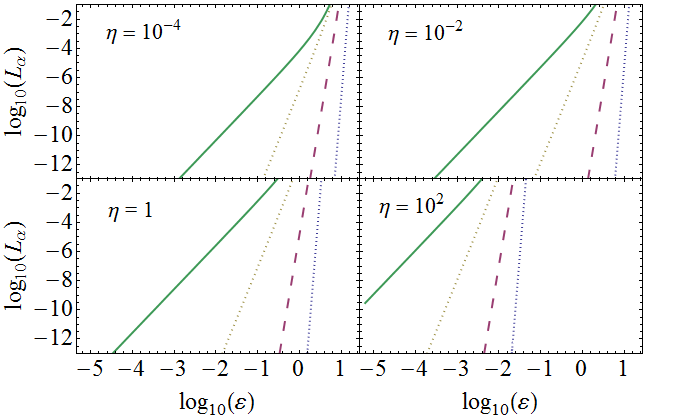
Figure 2: (Color online) The upper bound $L_{\alpha}$ for $\|A_{x}\|=\|A_{y}\|=\|A_{z}\|$ according to Eqs. (43) in the isotropic case, i.e., $\eta_{x}=\eta_{y}=\eta_{z}$, is given as a function of $\varepsilon$ for various number of pulses $N_{1}=N_{2}=N\in\{2,6,16,34\}$, at fixed values of $\eta_{\alpha}$. In each panel the curves become steeper as $N$ increases.

We also investigated the case where $\eta_{x}=\eta_{y}\neq\eta_{z}$ and how the parities of $N_{1}$ and $N_{2}$ affect the bounds. In Fig. 3 and Fig. 4, we plotted two cases. The first is where both $N_{1}$ and $N_{2}$ are even, which are represented by the thick lines. The second is where $N_{1}$ and $N_{2}$ are either even or odd, which are represented by the thin lines. We picked $\eta_{z}$ to be $10^{-2}$ for all the plots and $\eta_{x}=\eta_{y}\in\{10^{-4},10^{-2},1,10^{2}\}$. Since $\eta_{z}$ is fixed, we also fixed the values of $N_{2}$ for the two cases. We picked $N_{2}$ to be 10 in the first case and 9 in the second case to explore the effect of parity. We varied the value of $N_{1}$ based on the values $\eta_{x}$ and $\eta_{y}$. We can see from the figures that in the majority of cases, the parities of $N_{1}$ and $N_{2}$ only change the decoupling order by 1 or do not change it at all, so the bounds do not vary much. However, when $N_{1}$ is small compared to $N_{2}$, the parities can change the bounds nontrivially as seen in the top left panels of Fig. 3 and Fig. 4. We can also see this from Table 1. When $N_{1}$ is small compared to $N_{2}$, the decoupling orders of $\sigma_{y}$ and $\sigma_{z}$ can decrease considerably when $N_{1}$ switches between even and odd values.

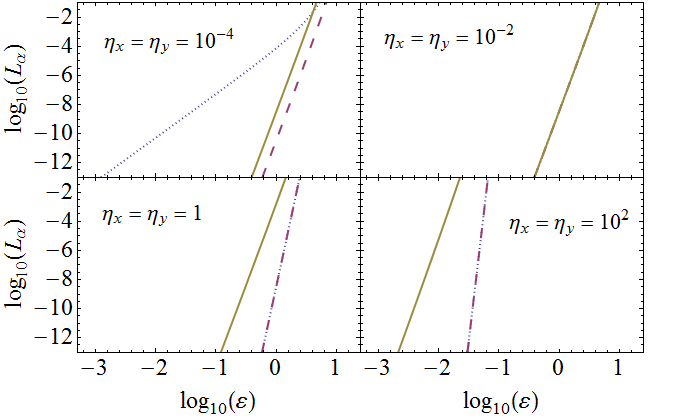
Figure 3: (Color online) The upper bounds for $\|A_{x}\|$ (dotted lines), $\|A_{y}\|$ (dashed lines) and $\|A_{z}\|$ (filled lines) according to Eq. (43) are depicted. Here $N_{2}$ is $10$. The values of $N_{1}$ in the four panels going from left to right and top to bottom are $2,10,18$ and $34$. The value of $\eta_{z}=10^{-2}$.

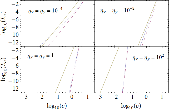
Figure 4: (Color online) The upper bounds for $\|A_{x}\|$ (dotted lines), $\|A_{y}\|$ (dashed lines) and $\|A_{z}\|$ (filled lines) according to Eqs. (43) are depicted. We make $N_{2}$ to be $9$ in this case. The values of $N_{1}$ in the four panels going from left to right and top to bottom are $3,10,19$ and $34$. The value of $\eta_{z}=10^{-2}$ as in the previous case.

Equation (43) allows us to establish tight bounds on the representation of the unitary time evolution as given in Eq. (30). In subsection IV.1 we use this fact to establish a bound on the trace-norm distance between the unperturbed qubit state and the protected qubit state.

III.2 NUDD

If we were to use the same method for NUDD for $m$ qubits as we did in the QDD case for one qubit, we would need to consider $2^{(3^{m})}$ cases based on the parities of $n_{\vec{\mu}}$. Recall that $n_{\vec{\mu}}$ indicates how many times $\widehat{\sigma}_{\vec{\mu}}\otimes B_{\vec{\mu}}$ appears in $(\widehat{\sigma}_{\vec{\mu}_{n}}\otimes B_{\vec{\mu}_{n}})\cdots(\widehat{\sigma}_{\vec{\mu}_{1}}\otimes B_{\vec{\mu}_{1}})$; Eq. (26d). To simplify the analysis, unlike the QDD case, we do not address each error term separately.

Any operator acting on the space of $m$ qubits can be expanded in the $\{\sigma_{\vec{\mu}}\}$ basis. Generalizing the QDD case [Eq. (30)] we can thus write

$$U(T)=\sum_{\vec{\mu}\in{D_{m}}}\widehat{\sigma}_{\vec{\mu}}\otimes A_{\vec{\mu}}(T),$$ (47)

where $\widehat{\sigma}_{\vec{\mu}}$ and $D_{m}$ were defined in Eqs. (19). Eq. (47) provides another way to organize the terms in Eq. (LABEL:nUseries). We introduce the upper bounding series $S_{\vec{\mu}}$ for each $A_{\vec{\mu}}$ such that

$${\color[rgb]{0,0,0}\|A_{\vec{\mu}}(T)\|} {\color[rgb]{0,0,0}\leq} {\color[rgb]{0,0,0}S_{\vec{\mu}}(T)}$$ (48a)

$$S_{\text{N}}(T) = \sum_{\vec{\mu}\in D_{m}}S_{\vec{\mu}}(T)$$ (48b)

holds. Below we construct this series explicitly. Let

$$\vec{0} := \{0,\dots,0\}$$ (49a)

$${\cal K} := {D_{m}}\backslash\vec{0}.$$ (49b)

Since $\widehat{\sigma}_{\vec{0}}$ is the all-identity term, it is the term that causes no errors; its corresponding bounding series is $S_{\vec{0}}(T)$. On the other hand, every $\widehat{\sigma}_{\vec{\mu}}$ with $\vec{\mu}\in{\cal K}$ is an error term with corresponding bounding series $S_{\vec{\mu}}(T)$. For later use, we note that $S_{\vec{0}}(0)=1$ and $S_{\vec{\mu}}(0)=0$ for all $\vec{\mu}\in{\cal K}$.

In order to derive bounds we first recall that $U(T)$ from Eq. (25) is the solution of the Schrödinger equation

$$\partial_{T}U(T) = -iH(T)U(T)$$ (50a)

$$= -i\left[\sum_{\vec{\mu}\in D_{m}}f_{\vec{\mu}}(t/T)\widehat{\sigma}_{\vec{\mu}}B_{\vec{\mu}}\right]U(T)$$ (50b)

with $U(0)=\mathbb{1}$. Eq. (50b) generates exactly all terms of the series of $U(T)$. Thus, in order to obtain the series for $S_{\text{N}}(T)$ all we need to do is to replace $-i\to|-i|=1$, $f_{\vec{\mu}}\to|f_{\vec{\mu}}|=1$, $\widehat{\sigma}_{\vec{\mu}}\to\|\widehat{\sigma}_{\vec{\mu}}\|=1$, and $B_{\vec{\mu}}\to\|B_{\vec{\mu}}\|=J_{\vec{\mu}}$ on the right hand side. This provides us with the generating differential equation for the bounding series

$$\partial_{T}S_{\text{N}}(T)=\left[\sum_{\vec{\mu}\in D_{m}}J_{\vec{\mu}}\right]S_{\text{N}}(T).$$ (51)

Its integration from $S_{\text{N}}(0)=1$ recovers the previous result (29) precisely.

In analogy, the differential equation for each $A_{\vec{\mu}}(T)$ reads

$$\partial_{T}A_{\vec{\mu}}(T)=-i\left[\sum_{\vec{\nu}\in D_{m}}f_{\vec{\mu}\oplus\vec{\nu}}(t/T)R_{\vec{\mu}\oplus\vec{\nu};\vec{\nu}}B_{\vec{\mu}\oplus\vec{\nu}}\right]A_{\vec{\nu}}(T),$$ (52)

where, as before, $\oplus$ stands for sums modulo 2. Note that addition and subtraction are equivalent modulo 2: $\vec{\mu}\oplus\vec{\nu}=\vec{\mu}\ominus\vec{\nu}$. It is essential that the sums modulo 2 in $\{(0,0),(1,0),(1,1),(0,1)\}$ faithfully reproduce the spin algebra of the identity and the Pauli matrices except for factors of $\pm i$, which are collected in $R_{\vec{\mu}\oplus\vec{\nu};\vec{\nu}}$. Replacing operators by their norms and complex numbers by their moduli on the right hand side yields the generating differential equation for the bounding series $S_{\vec{\mu}}$ satisfying Eq. (48a),

$$\partial_{T}S_{\vec{\mu}}(T)=\left[\sum_{\vec{\nu}\in D_{m}}J_{\vec{\mu}\oplus\vec{\nu}}\right]S_{\vec{\nu}}(T).$$ (53)

Unfortunately, the set of differential equations (53) is still too difficult to be solved generally. Hence we aim at a looser bound by defining

$$J_{1} := \max_{\vec{\mu}\in\mathcal{K}}J_{\vec{\mu}}$$ (54a)

$$\eta := \frac{J_{1}}{J_{\vec{0}}}$$ (54b)

$$\varepsilon := J_{\vec{0}}T.$$ (54c)

If we substitute $J_{1}$ for each $J_{\vec{\mu}}$ with $\vec{\mu}\in\mathcal{K}$ we obtain one bounding series $S_{1}(T)$ for all $S_{\vec{\mu}}(T)=S_{1}(T)$. To see this we insert $S_{1}(T)=S_{\vec{\mu}}(T)$ on the right hand side of Eq. (53) yielding

$$\partial_{T}S_{\vec{0}}(T) = J_{\vec{0}}S_{\vec{0}}(T)+\gamma J_{1}S_{1}(T)$$ (55a)

$$\partial_{T}S_{\vec{\mu}}(T) = J_{\vec{0}}S_{1}(T)+J_{1}S_{\vec{0}}(T)+(\gamma-1)J_{1}S_{1}(T)\qquad$$ (55b)

where $\vec{\mu}\in\mathcal{K}$ and $\gamma:=4^{m}-1=|\mathcal{K}|$ is the number of non-identity terms. The first term on the right hand side of (55a) results from $\vec{0}=\vec{0}\oplus\vec{0}$, the second from $\vec{\nu}=\vec{0}\oplus\vec{\nu}$ for $\vec{\nu}\in\mathcal{K}$. The first term on the right hand side of (55b) results from $\vec{0}=\vec{\mu}\oplus\vec{\mu}$, the second from $\vec{\mu}=\vec{\mu}\oplus\vec{0}$, and the third from $\vec{\mu}\oplus\vec{\nu}$ where $\vec{\nu}\in\mathcal{K}\backslash\vec{\mu}$. There are $\gamma-1$ terms of the latter kind, independent of $\vec{\mu}$. This independence implies the equality of all $S_{\vec{\mu}}(T)$ for $\vec{\mu}\in\mathcal{K}$ because they all start at the same value $S_{\vec{\mu}}(0)=0$. Thus, replacing Eq. (55b), we have

$$\partial_{T}S_{1}(T)=J_{\vec{0}}S_{1}(T)+J_{1}S_{\vec{0}}(T)+(\gamma-1)J_{1}S_{1}(T)$$ (56)

which, together with Eq. (55a), constitutes a two-dimensional set of linear differential equations. The two eigenvalues of the corresponding matrix are $\lambda_{+}=J_{\vec{0}}+\gamma J_{1}$ and $\lambda_{-}=J_{\vec{0}}-J_{1}$ so that the general solution reads $S_{1}(T):=A\exp(\lambda_{+}T)+B\exp(\lambda_{-}T)$ with coefficients $A$ and $B$. The initial conditions $S_{\vec{0}}(0)=1$ and $S_{1}(0)=0$ imply $\partial_{T}S_{1}(0)=J_{1}$ from which $A$ and $B$ are determined to yield

$$S_{1}(T)=\frac{\exp(J_{\vec{0}}T)}{\gamma+1}(\exp(\gamma J_{1}T)-\exp(-J_{1}T)).$$ (57)

The bounding series of the sum of all error terms is given by $S_{\mathcal{K}}(T):=\gamma S_{1}(T)$ which reads

$$S_{\mathcal{K}}(T)=\frac{\gamma\exp(J_{\vec{0}}T)}{\gamma+1}(\exp(\gamma J_{1}T)-\exp(-J_{1}T)).$$ (58)

This result is the bounding series for all error terms in NUDD.

We define

$$p_{k} := \frac{1}{k!}\frac{\partial^{k}}{\partial T^{k}}S_{\mathcal{K}}{\Big{|}}_{T=0}$$ (59a)

$$\Delta_{N} := \sum_{k=N+1}^{\infty}p_{k}T^{k},$$ (59b)

and

$$d_{\min}:=\min_{1\leq i\leq 2m}\{N_{i}^{\prime}\}$$ (60)

be the decoupling order of the NUDD sequence Jiang and Imambekov (2011). Since $\|A_{\vec{\mu}}\|\leq S_{\vec{\mu}}(T)$, we have

$$\sum_{\vec{\mu}\in\mathcal{K}}\|A_{\vec{\mu}}\|\leq\sum_{\vec{\mu}\in\mathcal{K}}S_{\vec{\mu}}(T)\leq S_{\mathcal{K}}(T),$$ (61)

and hence

$$\sum_{\vec{\mu}\in\mathcal{K}}\|A_{\vec{\mu}}\|\leq\Delta_{d_{\min}}.$$ (62)

By Taylor-expanding Eq. (58) we can write $S_{\mathcal{K}}(T)$ and thus $\Delta_{d}$ as an infinite series in terms of $\varepsilon$ and $\eta$ of Eqs. (54c) and (54b). We do not write the result explicitly, but the formula (58) for $S_{\mathcal{K}}(T)$ is simple enough to allow the bounds to be computed easily with any computer algebra program. This is our first key result for the NUDD sequence.

To leading order in $\varepsilon$, we find

$$\Delta_{d}=g_{d+1}(\eta,m)\varepsilon^{d+1}+\mathcal{O}(\varepsilon^{d+2}),$$ (63)

where

$$g_{l}(\eta,m):=(1-4^{-m})\frac{(1-\eta+4^{m}\eta)^{l}-(1-\eta)^{l}}{l!}.$$ (64)

In Fig. 5 we include plots of $\Delta_{d_{\min}}$ as a function of $\varepsilon$ for various values of ${d_{\min}}$ and $\eta$. We can see that, as expected, the behavior of $\Delta_{d_{\min}}$ is similar to that of $L_{\alpha}$ in the QDD case.

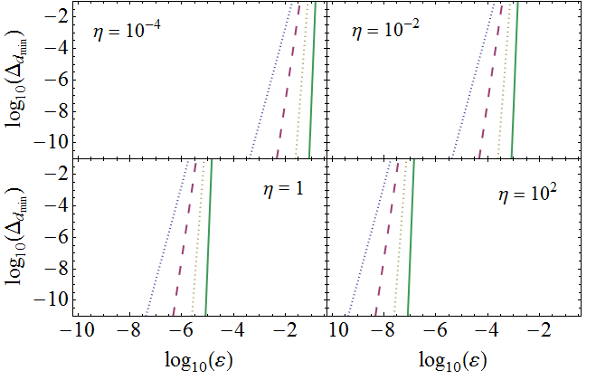
Figure 5: (Color online) The upper bound $\Delta_{d_{\min}}$ for $\sum_{\vec{\mu}\in\mathcal{K}}\|A_{\vec{\mu}}\|$ is given as a function of $\varepsilon$ for various pulse numbers ${\color[rgb]{0,0,0}d_{\min}}\in\{5,10,20,40\}$, at fixed values of $\eta$, and for $m=10$. In each panel the curves become steeper as $d_{\min}$ increases.

IV Distance bound

IV.1 QDD

Next, we shall use the bounds on the bath operators $A_{x},A_{y}$ and $A_{z}$ to derive a bound on the trace-norm distance

$$D[\rho_{\text{S}}(T),\rho_{\text{S}}^{0}(T)]={\color[rgb]{0,0,0}\frac{1}{2}\big{\|}\rho_{\text{S}}(T)-\rho_{\text{S}}^{0}(T)\big{\|}_{1}}$$ (65)

between the actual qubit state

$$\rho_{\text{S}}(T):=\mbox{tr}_{\text{B}}[\rho_{\text{SB}}(T)],$$ (66)

and the “error-free” qubit state

$$\rho_{\text{S}}^{0}(T):=\mbox{tr}_{\text{B}}[\rho_{\text{SB}}^{0}(T)]$$ (67)

where $\rho_{\text{SB}}^{0}(T)$ is the time-evolved state of the whole qubit-bath system without coupling between the qubit and the bath, and $\mbox{tr}_{\text{B}}$ denotes the partial trace over the bath degrees of freedom. The trace norm $\|A\|_{1}$ is the trace of $(A^{\dagger}A)^{1/2}$. The trace-norm distance $D$ is the standard distance measure between density matrices Nielsen and Chuang (2000). The method we employ here is similar to the one in Ref. Uhrig and Lidar (2010). We consider an initial state

$$\rho_{\text{SB}}^{0}(0)=|\psi\rangle\langle\psi|\otimes\rho_{\text{B}}$$ (68)

in which the qubit is in a pure state $|\psi\rangle$ and the bath is in an arbitrary state $\rho_{\text{B}}$ (e.g., a mixed thermal equilibrium state). The initial state evolves to $\rho_{\text{SB}}(T)=U(T)\rho_{\text{SB}}^{0}(0)U^{\dagger}(T)$ when the qubit and the bath are coupled, or to $\rho_{\text{SB}}^{0}(T)={[\mathbb{1}}_{\text{S}}\otimes U_{\text{B}}(T){]}\rho_{\text{SB}}^{0}(0){[\mathbb{1}}_{\text{S}}\otimes U_{\text{B}}^{\dagger}(T){]}$ when the qubit is isolated from its environment. The unitary bath time-evolution operator without coupling reads

$$U_{\text{B}}(T):=\exp(-iTB_{0})$$ (69)

where $B_{0}$ is the bath term in Eq. (5).

Let us first define the bath correlation functions

$$b_{\alpha\beta}(T):=\mbox{tr}[A_{\alpha}(T)\rho_{\text{B}}A_{\beta}^{\dagger}(T)]$$ (70)

where $\alpha,\beta\in\{0,x,y,z\}$. To simplify the notation, we will omit the time dependence $T$ in $b_{\alpha\beta}(T)$ and $A_{\alpha}(T)$ from now on. Computation yields (see Appendix B.1)

$$D[\rho_{\text{S}}(T),\rho_{\text{S}}^{0}(T)] \leq |b_{xx}+b_{yy}+b_{zz}|$$ (71)

$$+\frac{1}{2}\sum_{\alpha,\beta\in\{0,x,y,z\}}(|b_{\alpha\beta}|-|b_{00}|).\quad$$

We know from the unitarity of $U$ and Eq. (30) that

$${\mathbb{1}} = U^{\dagger}(T)U(T)$$

$$= {\mathbb{1}}_{\text{S}}\otimes\sum_{\alpha\in\{0,x,y,z\}}A_{\alpha}^{\dagger}A_{\alpha}$$

$$\,\,\,\,\,\,+\sum_{\alpha\in\{x,y,z\}}\sigma_{\alpha}\otimes(A_{\alpha}^{\dagger}A_{0}+A_{0}^{\dagger}A_{\alpha}+i[A_{\beta}^{\dagger},A_{\gamma}]),$$

where in the last sum $\{\beta,\gamma\}$ are adjusted to $\alpha$ so that $\{\alpha,\beta,\gamma\}$ is a cyclic permutation of $\{x,y,z\}$. Therefore we have

$${\mathbb{1}} = A_{0}^{\dagger}A_{0}+A_{x}^{\dagger}A_{x}+A_{y}^{\dagger}A_{y}+A_{z}^{\dagger}A_{z},$$ (73a)

$$0 = A_{x}^{\dagger}A_{0}+A_{0}^{\dagger}A_{x}+iA_{y}^{\dagger}A_{z}-iA_{z}^{\dagger}A_{y},$$ (73b)

$$0 = A_{y}^{\dagger}A_{0}+A_{0}^{\dagger}A_{y}+iA_{z}^{\dagger}A_{x}-iA_{x}^{\dagger}A_{z},$$ (73c)

$$0 = A_{z}^{\dagger}A_{0}+A_{0}^{\dagger}A_{z}+iA_{x}^{\dagger}A_{y}-iA_{y}^{\dagger}A_{x}.$$ (73d)

It follows from Eq. (73a) that $\langle i|\sum_{\alpha\in\{0,x,y,z\}}A_{\alpha}^{\dagger}A_{\alpha}|i\rangle=1$ for all normalized states $|i\rangle$, and thus

$$\langle i|A_{0}^{\dagger}A_{0}|i\rangle=\|A_{0}|i\rangle\|^{2}\leq 1$$ (74)

because $\langle i|\sum_{\alpha\in\{x,y,z\}}A_{\alpha}^{\dagger}A_{\alpha}|i\rangle=\sum_{\alpha\in\{x,y,z\}}\|A_{\alpha}|i\rangle\|^{2}$ is nonnegative. In particular, we know that

$$\|A_{0}\|\leq 1.$$ (75)

To obtain a bound on the functions $b_{\alpha\beta}$ we use the following general correlation functions inequality (see Ref. Uhrig and Lidar (2010) for a proof)

$$|\mbox{tr}[Q\rho_{\text{B}}Q^{\prime}]|\leq\|Q\|\|Q^{\prime}\|,$$ (76)

which holds for arbitrary bounded bath operators $Q,Q^{\prime}$. Using Eq. (75) , Eq. (76), and the bounds (43) in Eq. (71) yields

$$D[\rho_{\text{S}}(T),\rho_{\text{S}}^{0}(T)]$$ (77b)

$$\leq \|A_{x}\|+\|A_{y}\|+\|A_{z}\|+\|A_{x}\|^{2}+\|A_{y}\|^{2}+\|A_{z}\|^{2}$$

$${}+\|A_{x}\|\|A_{y}\|+\|A_{y}\|\|A_{z}\|+\|A_{x}\|\|A_{z}\|$$

$$\leq L_{x}+L_{y}+L_{z}+L_{x}^{2}+L_{y}^{2}+L_{z}^{2}+L_{x}L_{y}+L_{y}L_{z}$$

$${}+L_{x}L_{z}$$

$$= \Delta_{d_{x}}^{(3)}+\Delta_{d_{x}}^{(4)}+\Delta_{d_{y}}^{(2)}+\Delta_{d_{y}}^{(5)}+\Delta_{d_{z}}^{(1)}+\Delta_{d_{z}}^{(6)}$$

$${}+(\Delta_{d_{x}}^{(3)})^{2}+(\Delta_{d_{x}}^{(4)})^{2}+(\Delta_{d_{y}}^{(2)})^{2}+(\Delta_{d_{y}}^{(5)})^{2}+(\Delta_{d_{z}}^{(1)})^{2}$$

$${}+(\Delta_{d_{z}}^{(6)})^{2}+2\Delta_{d_{x}}^{(3)}\Delta_{d_{x}}^{(4)}+2\Delta_{d_{y}}^{(2)}\Delta_{d_{y}}^{(5)}+2\Delta_{d_{z}}^{(1)}\Delta_{d_{z}}^{(6)}$$

$${}+\Delta_{d_{x}}^{(3)}\Delta_{d_{y}}^{(2)}+\Delta_{d_{x}}^{(3)}\Delta_{d_{y}}^{(5)}+\Delta_{d_{x}}^{(4)}\Delta_{d_{y}}^{(2)}+\Delta_{d_{x}}^{(4)}\Delta_{d_{y}}^{(5)}$$

$${}+\Delta_{d_{y}}^{(2)}\Delta_{d_{z}}^{(1)}+\Delta_{d_{y}}^{(2)}\Delta_{d_{z}}^{(6)}+\Delta_{d_{y}}^{(5)}\Delta_{d_{z}}^{(1)}+\Delta_{d_{y}}^{(5)}\Delta_{d_{z}}^{(6)}$$

$${}+\Delta_{d_{x}}^{(3)}\Delta_{d_{z}}^{(1)}+\Delta_{d_{x}}^{(3)}\Delta_{d_{z}}^{(6)}+\Delta_{d_{x}}^{(4)}\Delta_{d_{z}}^{(1)}+\Delta_{d_{x}}^{(4)}\Delta_{d_{z}}^{(6)}.$$

This is the rigorous bound on the trace-norm distance and hence our second key result for QDD.

Using Eq. (46b), one can rewrite this bound in terms of $\varepsilon$ and $\vec{\eta}$, which we do not write out here for brevity.

In explicit calculations the leading order in $\varepsilon$ will dominate for $\varepsilon\to 0$. Then only the first line in Eq. (77) plays a role, since all other terms are of higher order. Hence we have

$$D[\rho_{\text{S}}(T),\rho_{\text{S}}^{0}(T)] \leq [g_{d_{x}+1}^{(3)}(\vec{\eta})+g_{d_{x}+1}^{(4)}(\vec{\eta})]\varepsilon^{d_{x}+1}$$ (78)

$$+[g_{d_{y}+1}^{(2)}(\vec{\eta})+g_{d_{y}+1}^{(5)}(\vec{\eta})]\varepsilon^{d_{y}+1}$$

$$+[g_{d_{z}+1}^{(1)}(\vec{\eta})+g_{d_{z}+1}^{(6)}(\vec{\eta})]\varepsilon^{d_{z}+1}$$

$$+\mathcal{O}(\varepsilon^{\min_{\alpha\in\{x,y,z\}}\{d_{\alpha}\}+2}).$$

Equation (78) is our third key QDD result. It shows that the QDD bound is dominated by the channel with the smallest decoupling order $d_{\alpha}$, as was expected intuitively.

IV.2 NUDD

We consider an initial state

$$\rho_{\text{SB}}^{0}(0)=|\psi\rangle\langle\psi|\otimes\rho_{\text{B}}$$ (79)

where $|\psi\rangle$ is the state of the $m$-qubit system. The initial state evolves to $\rho_{\text{SB}}(T)=U(T)\rho_{\text{SB}}^{0}(0)U^{\dagger}(T)$ when the qubit and the bath are coupled, or to $\rho_{\text{SB}}^{0}(T)={[\mathbb{1}_{\text{S}}\otimes U_{\text{B}}(T)]\rho_{\text{SB}}^{0}(0)[\mathbb{1}_{\text{S}}\otimes U_{\text{B}}^{\dagger}(T)]}$ when the qubit is isolated from its environment. The unitary bath time-evolution operator without coupling reads

$$U_{\text{B}}(T):=\exp(-iTB_{\vec{0}})$$ (80)

where $B_{\vec{0}}$ is the bath operator that corresponds to the identity system operator. We know from the unitarity of $U(T)$ and Eq. (47) that

$$\sum_{\vec{\mu}\in{D_{m}}}A_{\vec{\mu}}^{\dagger}A_{\vec{\mu}}={\mathbb{1}}.$$ (81)

Following the same steps as in the QDD case yields

$$\|A_{\vec{0}}\|\leq 1.$$ (82)

Explicit computation (see Appendix B.2) as in the QDD case shows that

$$D[\rho_{\text{S}}(T),\rho_{\text{S}}^{0}(T)]\leq\Big{(}\sum_{\vec{\mu}\in{\mathcal{K}}}\|A_{\vec{\mu}}\|\Big{)}^{2}+\|A_{\vec{0}}\|\sum_{\vec{\mu}\in{\mathcal{K}}}\|A_{\vec{\mu}}\|.$$ (83)

We use the bounds on the operators $A_{\vec{\mu}}$ to derive a bound on the trace norm distance between $\rho_{\text{SB}}(T)$ and $\rho_{\text{SB}}^{0}(T)$. Substituting Eq. (62) and Eq. (82) into Eq. (83), we conclude that

$$D[\rho_{\text{S}}(T),\rho_{\text{S}}^{0}(T)]\leq\Delta_{d_{\min}}^{2}+\Delta_{d_{\min}},$$ (84)

where $\Delta_{d_{\min}}$ is the bound presented in Eq. (59b). The bound is dominated by $\Delta_{d_{\min}}$ which is the leading order term for $\varepsilon\to 0$. By expanding $\Delta_{d_{\min}}$ we find for the leading order term

$$D[\rho_{\text{S}}(T),\rho_{\text{S}}^{0}(T)]\leq g_{{d_{\min}}+1}(\eta,m)\varepsilon^{{d_{\min}}+1}+{\mathcal{O}(\varepsilon^{{d_{\min}}+2})}.$$ (85)

Equation (85) is our second key result for NUDD.

V Conclusions

We have derived and presented rigorous performance bounds for the QDD and NUDD sequences, respectively. These sequences, which build on the UDD sequence, protect a qubit or system of qubits from general decoherence, under the assumptions that the pulses are instantaneous and the bath operators are bounded in operator norm. Our key bounds are given in Eq. (77) for QDD and in Eq. (84) for NUDD. The leading order terms are identified in Eq. (78) (for QDD) and Eq. (85) (for NUDD). These results show that if the total sequence time is fixed, we can make the error $D[\rho_{\text{S}}(T),\rho_{\text{S}}^{0}(T)]$ arbitrarily small by increasing the number of pulses at each UDD level comprising the QDD or NUDD sequences.

When instead the minimum pulse interval is fixed, we expect that, just as in the case of UDD Uhrig and Lidar (2010), there will be an optimal sequence order, beyond which performance starts to decrease. A rigorous study of this aspect of QDD and NUDD is an interesting topic for a future investigation. We hope that the results presented here will inspire experimental tests of the QDD and NUDD sequences in physical systems with bath spectral densities exhibiting relatively hard high frequency cutoffs, a condition which corresponds to our key assumptions [Eqs. (6),(17)] of bounded bath operators.

Appendix A Bounding polynomials

The polynomials that appear in the Taylor expansions of the bounding functions $S_{j}(\varepsilon,\vec{\eta})$ are:

$$g_{l}^{(1)}(\vec{\eta}) = \frac{1}{8l!}[(1+\eta_{x}+\eta_{y}+\eta_{z})^{l}+(1-\eta_{x}+\eta_{y}+\eta_{z})^{l}$$

$${}+(1+\eta_{x}-\eta_{y}+\eta_{z})^{l}+(1-\eta_{x}-\eta_{y}+\eta_{z})^{l}$$

$${}-(1+\eta_{x}+\eta_{y}-\eta_{z})^{l}-(1-\eta_{x}+\eta_{y}-\eta_{z})^{l}$$

$${}-(1+\eta_{x}-\eta_{y}-\eta_{z})^{l}-(1-\eta_{x}-\eta_{y}-\eta_{z})^{l}]$$

(86)

$$g_{l}^{(2)}(\vec{\eta}) = \frac{1}{8l!}[(1+\eta_{x}+\eta_{y}+\eta_{z})^{l}+(1-\eta_{x}+\eta_{y}+\eta_{z})^{l}$$

$${}-(1+\eta_{x}-\eta_{y}+\eta_{z})^{l}-(1-\eta_{x}-\eta_{y}+\eta_{z})^{l}$$

$${}+(1+\eta_{x}+\eta_{y}-\eta_{z})^{l}+(1-\eta_{x}+\eta_{y}-\eta_{z})^{l}$$

$${}-(1+\eta_{x}-\eta_{y}-\eta_{z})^{l}-(1-\eta_{x}-\eta_{y}-\eta_{z})^{l}]$$

(87)

$$g_{l}^{(3)}(\vec{\eta}) = \frac{1}{8l!}[(1+\eta_{x}+\eta_{y}+\eta_{z})^{l}+(1-\eta_{x}+\eta_{y}+\eta_{z})^{l}$$

$${}-(1+\eta_{x}-\eta_{y}+\eta_{z})^{l}-(1-\eta_{x}-\eta_{y}+\eta_{z})^{l}$$

$${}-(1+\eta_{x}+\eta_{y}-\eta_{z})^{l}-(1-\eta_{x}+\eta_{y}-\eta_{z})^{l}$$

$${}+(1+\eta_{x}-\eta_{y}-\eta_{z})^{l}+(1-\eta_{x}-\eta_{y}-\eta_{z})^{l}]$$

(88)

$$g_{l}^{(4)}(\vec{\eta}) = \frac{1}{8l!}[(1+\eta_{x}+\eta_{y}+\eta_{z})^{l}-(1-\eta_{x}+\eta_{y}+\eta_{z})^{l}$$

$${}+(1+\eta_{x}-\eta_{y}+\eta_{z})^{l}-(1-\eta_{x}-\eta_{y}+\eta_{z})^{l}$$

$${}+(1+\eta_{x}+\eta_{y}-\eta_{z})^{l}-(1-\eta_{x}+\eta_{y}-\eta_{z})^{l}$$

$${}+(1+\eta_{x}-\eta_{y}-\eta_{z})^{l}-(1-\eta_{x}-\eta_{y}-\eta_{z})^{l}]$$

(89)

$$g_{l}^{(5)}(\vec{\eta}) = \frac{1}{8l!}[(1+\eta_{x}+\eta_{y}+\eta_{z})^{l}-(1-\eta_{x}+\eta_{y}+\eta_{z})^{l}$$

$${}+(1+\eta_{x}-\eta_{y}+\eta_{z})^{l}-(1-\eta_{x}-\eta_{y}+\eta_{z})^{l}$$

$${}-(1+\eta_{x}+\eta_{y}-\eta_{z})^{l}+(1-\eta_{x}+\eta_{y}-\eta_{z})^{l}$$

$${}-(1+\eta_{x}-\eta_{y}-\eta_{z})^{l}+(1-\eta_{x}-\eta_{y}-\eta_{z})^{l}]$$

(90)

$$g_{l}^{(6)}(\vec{\eta}) = \frac{1}{8l!}[(1+\eta_{x}+\eta_{y}+\eta_{z})^{l}-(1-\eta_{x}+\eta_{y}+\eta_{z})^{l}$$

$${}-(1+\eta_{x}-\eta_{y}+\eta_{z})^{l}+(1-\eta_{x}-\eta_{y}+\eta_{z})^{l}$$

$${}+(1+\eta_{x}+\eta_{y}-\eta_{z})^{l}-(1-\eta_{x}+\eta_{y}-\eta_{z})^{l}$$

$${}-(1+\eta_{x}-\eta_{y}-\eta_{z})^{l}+(1-\eta_{x}-\eta_{y}-\eta_{z})^{l}]$$

(91)

Appendix B Distance Bound Calculation

B.1 QDD

In this appendix we prove the bound on the trace-norm distance in Eq. (71). To simplify the notation, we let

$$P_{0}:=|\psi\rangle\langle\psi|.$$ (92)

Then

$$2D[\rho_{\text{S}}(T),\rho_{\text{S}}^{0}(T)]$$ (93b)

$$= \big{\|}\mbox{tr}_{\text{B}}\left[\rho_{\text{SB}}(T)-\rho_{\text{SB}}^{0}(T)\right]\big{\|}_{1}$$

$$= \big{\|}\mbox{tr}_{\text{B}}\left[U(T)\rho_{\text{SB}}^{0}(0)U^{\dagger}(T)\right]-\mbox{tr}_{\text{B}}\left[\rho_{\text{SB}}^{0}(0)\right]\big{\|}_{1}$$

$$= \left\|\mbox{tr}_{\text{B}}\left\{\left[\sum_{\alpha\in\{0,x,y,z\}}\sigma_{\alpha}\otimes A_{\alpha}\right](P_{0}\otimes\rho_{\text{B}})\right.\right.$$

$$\left.\left.\left[\sum_{\alpha\in\{0,x,y,z\}}\sigma_{\alpha}\otimes A_{\alpha}^{\dagger}\right]\right\}-P_{0}\right\|_{1}$$

$$= \big{\|}(b_{00}-1)P_{0}+b_{0x}P_{0}\sigma_{x}+b_{0y}P_{0}\sigma_{y}$$

$${}+b_{0z}P_{0}\sigma_{z}+b_{x0}\sigma_{x}P_{0}+b_{xx}\sigma_{x}P_{0}\sigma_{x}$$

$${}+b_{xy}\sigma_{x}P_{0}\sigma_{y}+b_{xz}\sigma_{x}P_{0}\sigma_{z}+b_{y0}\sigma_{y}P_{0}$$

$${}+b_{yx}\sigma_{y}P_{0}\sigma_{x}+b_{yy}\sigma_{y}P_{0}\sigma_{y}+b_{yz}\sigma_{y}P_{0}\sigma_{z}$$

$${}+b_{z0}\sigma_{z}P_{0}+b_{zx}\sigma_{z}P_{0}\sigma_{x}+b_{zy}\sigma_{z}P_{0}\sigma_{y}$$

$${}+b_{zz}\sigma_{z}P_{0}\sigma_{z}\big{\|}_{1}$$

$$\leq |b_{00}-1|+|b_{0x}|+|b_{0y}|+|b_{0z}|$$

$${}+|b_{x0}|+|b_{xx}|+|b_{xy}|+|b_{xz}|$$

$${}+|b_{y0}|+|b_{yx}|+|b_{yy}|+|b_{yz}|$$

$${}+|b_{z0}|+|b_{zx}|+|b_{zy}|+|b_{zz}|.$$

In going from Eq. (93b) to Inq. (93b), we used the triangle inequality, the unitary invariance of the trace norm, and the normalization of $|\psi\rangle$. This proves Eq. (71).

We require one last result:

$$\begin{split}&|b_{00}-1|=|\mbox{tr}[A_{0}\rho_{\text{B}}A_{0}^{\dagger}]-1|\\ &=|\mbox{tr}[A_{0}^{\dagger}A_{0}\rho_{\text{B}}]-1|\\ &=|\mbox{tr}\{[\mathbb{1}-A_{x}^{\dagger}A_{x}-A_{y}^{\dagger}A_{y}-A_{z}^{\dagger}A_{z}]\rho_{\text{B}}\}-1|\\ &=|\mbox{tr}[\rho_{\text{B}}]-\mbox{tr}[A_{x}\rho_{\text{B}}A_{x}^{\dagger}]-\mbox{tr}[A_{y}\rho_{\text{B}}A_{y}^{\dagger}]-\mbox{tr}[A_{z}\rho_{\text{B}}A_{z}^{\dagger}]|\\ &=|b_{xx}+b_{yy}+b_{zz}|,\end{split}$$ (94)

where we used cyclic invariance of the trace in $b_{\alpha\beta}$ together with Eq. (73a) and the normalization $\mbox{tr}[\rho_{\text{B}}]=1$. Eq. (71) now follows immediately from the triangle inequality.

B.2 NUDD

Here we prove Eq. (83) following the same steps as in the QDD case.

$$D[\rho_{\text{S}}(T),\rho_{\text{S}}^{0}(T)]$$ (95a)

$$= \big{\|}\mbox{tr}_{\text{B}}[\rho_{\text{SB}}(T)-\rho_{\text{SB}}^{0}(T)]\big{\|}_{1}$$

$$= \big{\|}\mbox{tr}_{\text{B}}[U(T)\rho_{\text{SB}}^{0}(0)U^{\dagger}(T)]-\mbox{tr}_{\text{B}}[\rho_{\text{SB}}^{0}(0)]\big{\|}_{1}$$

$$= \left\|\mbox{tr}_{\text{B}}\left\{\left[\sum_{\vec{\mu}\in\{0,1\}^{2m}}\sigma_{\vec{\mu}}A_{\vec{\mu}}\right](P_{0}\otimes\rho_{\text{B}})\right.\right.$$

$$\left.\left.\left[\sum_{\vec{\mu}\in\{0,1\}^{2m}}\sigma_{\vec{\mu}}A_{\vec{\mu}}^{\dagger}\right]\right\}-P_{0}\right\|_{1}$$

$$= \left\|\sum_{\vec{\mu}\in\{0,1\}^{2m}}\sum_{\vec{\nu}\in\{0,1\}^{2m}}\mbox{tr}(A_{\vec{\mu}}^{\dagger}\rho_{\text{B}}A_{\vec{\nu}})\sigma_{\vec{\mu}}P_{0}\sigma_{\vec{\nu}}-P_{0}\right\|_{1}$$

$$\leq |\mbox{tr}(A_{\vec{0}}^{\dagger}\rho_{\text{B}}A_{\vec{0}})-1|+\sum_{\vec{\mu}\in{\cal K}}\sum_{\vec{\nu}\in{\cal K}}|\mbox{tr}(A_{\vec{\mu}}^{\dagger}\rho_{\text{B}}A_{\vec{\nu}})|$$

$${}+\sum_{\vec{\mu}\in{\cal K}}{|}\mbox{tr}(A_{\vec{0}}^{\dagger}\rho_{\text{B}}A_{\vec{\mu}}){|}+\sum_{\vec{\mu}\in{\cal K}}{|}\mbox{tr}(A_{\vec{\mu}}^{\dagger}\rho_{\text{B}}A_{\vec{0}}){|}$$

$$\leq \sum_{\vec{\mu}\in{\cal K}}|\mbox{tr}(A_{\vec{\mu}}^{\dagger}\rho_{\text{B}}A_{\vec{\mu}})|+\sum_{\vec{\mu}\in{\cal K}}\sum_{\vec{\nu}\in{\cal K}}|\mbox{tr}(A_{\vec{\mu}}^{\dagger}\rho_{\text{B}}A_{\vec{\nu}})|$$

$${}+\sum_{\vec{\mu}\in{\cal K}}|\mbox{tr}(A_{\vec{0}}^{\dagger}\rho_{\text{B}}A_{\vec{\mu}})|+\sum_{\vec{\mu}\in{\cal K}}|\mbox{tr}(A_{\vec{\mu}}^{\dagger}\rho_{\text{B}}A_{\vec{0}})|$$

$${\leq} {\Big{(}\sum_{\vec{\mu}\in\mathcal{K}}\|A_{\vec{\mu}}\|\Big{)}^{2}+\sum_{\vec{\mu}\in\mathcal{K}}\|A_{\vec{\mu}}\|^{2}+2\|A_{\vec{0}}\|\sum_{\vec{\mu}\in\mathcal{K}}\|A_{\vec{\mu}}\|\qquad}$$

$$\leq 2\Big{(}\sum_{\vec{\mu}\in{\cal K}}\|A_{\vec{\mu}}\|\Big{)}^{2}+2\|A_{\vec{0}}\|\sum_{\vec{\mu}\in{\cal K}}\|A_{\vec{\mu}}\|.$$ (95b)

In the derivation we used the unitary invariance of the trace norm, triangle inequality, the normalization of $|\psi\rangle$, Eq. (76) and Eq. (81). The step from inequality (95a) to (95b) is not necessary, but loosens the bound for the sake of simplicity of the result.

References

- Nielsen and Chuang (2000) M. Nielsen and I. Chuang, Quantum Computation and Quantum Information (Cambridge University Press, Cambridge, England, 2000).
- M. S. Byrd and D. A. Lidar (2003) M. S. Byrd and D. A. Lidar, J. Mod. Optics, 50, 1285 (2003).
- Viola and Lloyd (1998) L. Viola and S. Lloyd, Phys. Rev. A, 58, 2733 (1998).
- Ban (1998) M. Ban, J. Mod. Optics, 45, 2315 (1998).
- Zanardi (1999) P. Zanardi, Phys. Lett. A, 258, 77 (1999).
- Viola et al. (1999) L. Viola, E. Knill, and S. Lloyd, Phys. Rev. Lett., 82, 2417 (1999).
- Byrd and Lidar (2001) M. S. Byrd and D. A. Lidar, Quant. Inf. Proc., 1, 19 (2001).
- Uhrig (2007) G. Uhrig, Phys. Rev. Lett., 98, 100504 (2007), Erratum, ibid 106, 129901 (2011).
- B. Lee (2008) S. D. S. B. Lee, W. M. Witzel, Phys. Rev. Lett., 100, 160505 (2008).
- Uhrig (2008) G. S. Uhrig, New J. Phys., 10, 083024 (2008), Erratum ibid 13, 059504 (2011).
- Yang and Liu (2008) W. Yang and R.-B. Liu, Phys. Rev. Lett., 101, 180403 (2008).
- Biercuk et al. (2009) M. Biercuk, H. Uys, A. VanDevender, N. Shiga, W. Itano, and J. Bollinger, Nature, 458, 996 (2009a).
- Biercuk et al. (2009) M. J. Biercuk, H. Uys, A. P. VanDevender, N. Shiga, W. M. Itano, and J. J. Bollinger, Phys. Rev. A, 79, 062324 (2009b).
- Uhrig and Lidar (2010) G. S. Uhrig and D. A. Lidar, Phys. Rev. A, 82, 012301 (2010).
- West et al. (2010) J. R. West, B. H. Fong, and D. A. Lidar, Phys. Rev. Lett., 104, 130501 (2010).
- Wang and Liu (2011) Z.-Y. Wang and R.-B. Liu, Phys. Rev. A, 83, 022306 (2011).
- Quiroz and Lidar (2011) G. Quiroz and D. A. Lidar, Phys. Rev. A, 84, 042328 (2011).
- Kuo and Lidar (2011) W.-J. Kuo and D. A. Lidar, Phys. Rev. A, 84, 042329 (2011).
- Jiang and Imambekov (2011) L. Jiang and A. Imambekov, (2011), eprint arXiv:1104.5021.
- Pasini and Uhrig (2011) S. Pasini and G. S. Uhrig, Phys. Rev. A, 84, 042336 (2011).