Pilotless Recovery of Clipped OFDM
Signals by Compressive Sensing over
Reliable Data Carriers

Abstract

In this paper we propose a novel form of clipping mitigation in OFDM using compressive sensing that completely avoids tone reservation and hence rate loss for this purpose. The method builds on selecting the most reliable perturbations from the constellation lattice upon decoding at the receiver, and performs compressive sensing over these observations in order to completely recover the temporally sparse nonlinear distortion. As such, the method provides a unique practical solution to the problem of initial erroneous decoding decisions in iterative ML methods, offering both the ability to augment these techniques and to solely recover the distorted signal in one shot.

I Introduction

Multicarrier signalling schemes such as Orthogonal Frequency Division Multiplexing (OFDM) have an inherent sensitivity to nonlinear distortion at all stages of the transmission process. To obtain information about the nonlinear temporal distortion in an OFDM signal, the majority of receiver-based mitigation techniques begin with observing the deviation of the equalized frequency domain variables from the discrete symbol constellation. As useful as this may be, a valid inconsistency is always persistently present. After all, it is the position of those very symbols in the frequency domain that ultimately entitle our decoding decisions, and should any of those symbols be perturbed outside their correct decision boundaries by nonlinear distortion, it will always be the case that any further reliance on these erroneous measurements might be resistent to further correction. Furthermore, refraining from using part of the deviations in recovering the distortion reduces the effectiveness of the mitigating algorithm.

Our major contributions are then to first suggest algorithms that can use a subset of the deviations in the frequency domain to dually avoid erroneous decisions and recover from the distortion with no theoretical sacrifice of given information and thus performance, and secondly to tailer the input model to these algorithms by selecting the most appropriate set of observations using a simplified procedure that models an actual Bayesian reliability measure. Although many scenarios and modifications apply to the methods herein, due to the limited space and the ongoing development of the presented concepts, we will restrict our discussion to mitigating distortion caused by clipping at the transmitter, and delay more elaborate applications to a further treatment.

Unless otherwise noted, frequency domain variables will be represented by uppercase italic letters while lower case letters will be reserved for time domain variables. The lower index in $\mathcal{X}_{i}$ will denote the $i^{th}$ constellation point amongst an M-ary alphabet $\mathcal{X}$ while $A_{i}(k)$ will be used for the $k^{th}$ scalar coefficient of the the $i^{th}$ column vector $A_{i}$ of matrix A. Furthermore, $\langle X(k)\rangle$ will denote a hard decoding operation which maps $X(k)$ back into $\mathcal{X}$. The standard notation of $x_{i:N}$ will be be used for the $i^{th}$ order statistic in a sample of $N$ random variables of a common probability density function [1]. Finally, we use $\mathbb{F}$ for Cumulative Distribution Functions (CDF) and F for unitary Fourier matrices.

II Transmission and Clipping Model

In an OFDM system, Serially incoming bits are mapped into an M-ary QAM alphabet $\{\mathcal{X}_{0},\mathcal{X}_{1},\ldots,\mathcal{X}_{M-1}\}$ and concatenated to form an $N$ dimensional data vector $X=[X(0)X(1)\cdots X(N-1)]^{T}$. The time-domain signal is obtained by an IFFT operation so that $x=\textbf{F}^{H}X$ where

$$F_{k}(\ell)=N^{-1/2}\,e^{-j2\pi k\ell/LN},\quad k,\ell\in{0,1,\ldots,LN-1}.$$

and $L$ is an oversampling factor. Since $x$ has a high peak to average power ratio (PAPR), the digital samples are subject to a magnitude limiter which saturates its operands to a value of $\gamma$, and hence instead of feeding $x$ to the power amplifier, we feed $\bar{x}$ where

$$\bar{x}(i)=\begin{cases}\gamma e^{\;j\theta_{x(i)}}\;&\mbox{if}\;|x(i)|>\gamma,\\ \,\,\,\,x(i)\;&\mbox{otherwise}\end{cases}$$ (1)

where $\theta_{x(i)}$ is the phase of $x(i)$. This soft limiting operation can be conveniently thought of as adding a peak-reducing signal $c$ to $x$ whereby its low-PAPR counterpart $\bar{x}=x+c$ is transmitted instead, and whereby $x$ can be re-generated at the receiver by estimating $c$. What’s more, by setting a typical clipping threshold $\gamma$ on $x$, $c$ is controllably sparse in time by the impulsive nature of $x$, and dense in frequency by the uncertainty principle. We will denote its temporal support by $\mathcal{I}_{c}=\{n:c(n)\neq 0\}$ and always maintain the practical assumption that $|\mathcal{I}_{c}|\ll N$.

In the frequency domain, this translates to transmitting $\bar{X}=X+C$, with complex coefficients that are now randomly pre-perturbed from the lattice $\mathcal{X}$, followed by additional random post-perturbations by the channel $\textbf{H}\!\!=\!\!\textbf{F}^{H}\Lambda\textbf{F}$ and additive noise samples $Z\sim\mathcal{CN}(0,\sigma_{Z}I_{N\times N})$ at the receiver, where the circulant channel H has been decomposed as such by virtue of the added cyclic prefix in OFDM signalling. At the receiver, this reads

$$Y=\Lambda\,\bar{X}+Z,$$ (2)

where we will make the practical assumption that the channel coefficients are known on its side. Consequently, $\bar{X}$ can be directly recovered scalar-wise from $Y$, i.e.

$$\hat{\bar{X}}(k) = \Lambda^{-1}_{k}(k)Y(k)$$ (3)

$$= X(k)+C(k)+\Lambda_{k}^{-1}(k)Z(k).$$

Let $D(k)\!\triangleq\!C(k)+\Lambda_{k}^{-1}(k)Z(k)$ denote the general distortion on the frequency domain sample $X(k)$. A naive ML decoder will now simply map $\hat{\bar{X}}(k)$ to the nearest constellation point $\mathcal{X}_{i^{*}}$ to recover $X(k)$, where $i^{*}(k)\triangleq\arg\min_{i}|\hat{\bar{X}}(k)-\mathcal{X}_{i}(k)|$, treating the clipping distortion as additive noise. Although such a hard-decoding scheme is very efficient at high SNR in the classical AWGN scenario, the clipping scenario, however, introduces another $\gamma$-dependent source of perturbation which is immune to any increase in SNR.

An intelligent ML decoder will hence have to iteratively update its decisions in the frequency domain based on the resulting waveforms in the time domain. Unfortunately, such a method will suffer from error propagation since a single faulty decision in frequency will generate a faulty estimate of $c$ in time which will be used to update the frequency perturbations in the next iteration and so on.

A direct countermeasure would be to refrain from using the tones at which the perturbations $D(k)$ are large and hence unreliable [6]. Although this should eliminate false positives in the time domain, the economy in tone usage severely limits the improvement offered by such an approach.

Alternatively, CS seems to be a very sensible solution to this problem. A partial observation of the frequency content of a sparse signal in the time domain is sufficient to recover $c$ and hence $C$ in one shot. This would certainly get around the problem of unreliable perturbations as CS algorithms can be totally blind to them and still offer near optimal signal reconstruction under mild conditions.

Fortunately, unlike our previous approach [2] of reserving a sufficient number of tones at the transmitter to recover $c$, and consequently reducing the transmission rate, we do not require any tone reservation in this method, and are completely free to choose any subset $\Omega_{m}$ from the $N$ data-carrying tones in order to reconstruct $c$ at the receiver. This freedom of choice opens up many possibilities in how to select particular adaptive subsets to optimize the CS performance as will be thoroughly discussed later on.

III Development of Compressive Sensing Models with No Tone Reservation

With the addition of $C$ to the data vector $X$, we suspect that a part of the data samples $X(k)$ will be severely perturbed to fall out of their corresponding decision regions $\mathcal{A}_{X(k)}$. Denote by $\Omega_{T}=\{k:\langle X(k)+C(k)\rangle=X(k)\}$ the subset of data tones in $\Omega$ in which the perturbations are not severe (i.e. do not cause crossing a decision boundary). At these locations, the equality in $\langle\bar{X}(k)\rangle=X(k)$ is true and hence $C_{\Omega_{T}}=\bar{X}_{\Omega_{T}}-\langle\bar{X}_{\Omega_{T}}\rangle$ at the transmitter. More generally,

$$C=\textbf{S}_{\Omega_{T}}\left(\bar{X}-\langle\bar{X}\rangle\right)+\textbf{S}_{\bar{\Omega}_{T}}\left(\bar{X}-X\right)$$ (4)

where $\textbf{S}_{\Omega_{T}}$ is an $N\!\times\!N$ diagonal and binary selection matrix, with $|\Omega_{T}|$ ones along its diagonal that extract the locations in the vector $\bar{X}-\langle\bar{X}\rangle$ according to the tone set $\Omega_{T}$ while nulling the others, and $\textbf{S}_{\bar{\Omega}_{T}}$ is its complement such that $\textbf{S}_{\Omega_{T}}\textbf{S}_{\bar{\Omega}_{T}}=\textbf{0}_{N\times N}$. Practically speaking, $\Omega_{T}$ constitutes the bigger part of the general tone set $\Omega$, with a probability of occupying at least $100\alpha\%$ of $\Omega$ equal to $\Pr(|\Omega_{T}|>\alpha N)\approx\sum_{\ell=0}^{N(1-\alpha)}{N\choose\ell}P_{e}^{\ell}(1-P_{e})^{N-\ell}$ for large constellations, where $P_{e}=2Q\left(\frac{d_{\min}}{2\sigma_{D}}\right)$. An essential part of OFDM signal recovery obviously constitutes finding this set, and correcting the distortion over $\bar{\Omega}_{T}$ to finally reach $\Omega_{T}=\Omega$.

Upon demodulation and decoding at the receiver, we are left with an estimate $\hat{\bar{X}}$ of the distorted data vector given in (3) along with its associated decoded vector $\langle\hat{\bar{X}}\rangle\in\mathcal{X}^{N}$. Taking the difference yields

$$\hat{\bar{X}}-\langle\hat{\bar{X}}\rangle = X+D-\langle X+D\rangle$$

$$= X+D-(\textbf{S}_{\Omega_{T}}X+\textbf{S}_{\bar{\Omega}_{T}}E)$$

where $\Omega_{T}$ now indexes the locations where $X(k)+D(k)$ remains within the correct ML decision region and $E$ represents the error vector resulting from incorrect decoding decisions at $\bar{\Omega}_{T}$. Multiplying both sides by $\textbf{S}_{\Omega_{T}}$ leaves us with

$$\textbf{S}_{\Omega_{T}}(\hat{\bar{X}}-\langle\hat{\bar{X}}\rangle) = \textbf{S}_{\Omega_{T}}X+\textbf{S}_{\Omega_{T}}D-\textbf{S}_{\Omega_{T}}(\textbf{S}_{\Omega_{T}}X+\textbf{S}_{\bar{\Omega}_{T}}E)$$ (5)

$$= \textbf{S}_{\Omega_{T}}X+\textbf{S}_{\Omega_{T}}D-\textbf{S}_{\Omega_{T}}X+\textbf{0}_{N\times 1}$$

$$= \textbf{S}_{\Omega_{T}}D$$

$$= \textbf{S}_{\Omega_{T}}\textbf{F}c+\textbf{S}_{\Omega_{T}}\Lambda^{-1}Z$$

where we have used the fact that $\textbf{S}_{\Omega_{T}}^{n}=\textbf{S}_{\Omega_{T}}$ for any positive integer $n$, and redundantly used $\textbf{S}_{\bar{\Omega}_{T}}$ on $E$ to show that $\textbf{S}_{\Omega_{T}}E=\textbf{S}_{\Omega_{T}}\textbf{S}_{\bar{\Omega}_{T}}E=\textbf{0}_{N\times 1}$. Note, however, that we do not require all of $\Omega_{T}$ to recover $c$, for obviously there would be no need for any recovery algorithm if we knew $\Omega_{T}$. Rather, we only require an arbitrary subset $\Omega_{m}\subseteq\Omega_{T}\subseteq\Omega$ of cardinality $|\Omega_{m}|<|\Omega_{T}|$ to correctly recover $c$ by CS. As a result, we can replace the equation above with

$$\textbf{S}_{\Omega_{m}}(\hat{\bar{X}}-\langle\hat{\bar{X}}\rangle) = \textbf{S}_{\Omega_{m}}\textbf{F}c+\textbf{S}_{\Omega_{m}}\Lambda^{-1}Z$$

$$= \Psi c+Z^{\prime}$$

where $\Psi\triangleq\textbf{S}_{\Omega_{m}}\textbf{F}$, $Z^{\prime}\triangleq\textbf{S}_{\Omega_{m}}\Lambda^{-1}Z$, and where we further let $Y^{\prime}\triangleq\textbf{S}_{\Omega_{m}}(\hat{\bar{X}}-\langle\hat{\bar{X}}\rangle)$ denote the observation vector of the differences over the tones in $\Omega_{m}$, nulled at the discarded measurements. This leads us to the lossless-rate CS model

$$Y^{\prime}_{\Omega_{m}}=\Psi_{\Omega_{m}}c+Z_{\Omega_{m}}^{\prime}.$$ (6)

where $Y^{\prime}_{\Omega_{m}}$ is the $|\Omega_{m}|$-dimensional vector collecting the nonzero coefficients in $Y^{\prime}$. Such a generic model can now be processed for $c$ using any compressive sensing technique, be it convex programming, greedy pursuit, or iterative thresholding, and a very flexible region for tradeoff exists in regard to performance and complexity. In any case, our subsequent objective is to scrutinize the general conditioning of the model itself by supplying our most reliable observations to the generic CS algorithm.

IV Cherry Picking $\Omega_{m}$

An essential question now is how one is to select among the $N\choose m$ possible constructions of $\Omega_{m}$. A general strategy of CS techniques is to select these $m$ tones randomly for near-optimum performance. Although possible in this scenario, such a strategy neglects the fact that our observations vary in their credibility and attest to wether they represent true frequency-domain measurements of $C$ or not since our assumption that $\hat{\bar{X}}(k)-\langle\hat{\bar{X}}(k)\rangle=D(k)$ is probabilistic. Furthermore, it neglects the fact that the estimation signal-to-noise-ratio $\mathbb{E}[\|\Psi_{\Omega_{m}}c\|_{2}^{2}]/\mathbb{E}[\|Z_{\Omega_{m}}^{\prime}\|_{2}^{2}]$ also varies with the channel gains $\{\Lambda_{k}(k)\}_{k\in\Omega_{m}}$, and that knowledge of these gains has an effect on our reliability estimates. With the receiver risking faulty decisions, it must devise a procedure to select the most reliable set of observations in which to sense over. This could be done based on the relative posterior probability of $D(k)$ equalling $\hat{\bar{X}}(k)-\langle\hat{\bar{X}}(k)\rangle$ to the probability of it equaling some other difference vector $\hat{\bar{X}}(k)-\mathcal{X}_{i,i\neq i^{*}}$. More precisely, let

$$\mathfrak{R}(k) = \log\frac{\Pr(\langle\hat{\bar{X}}(k)\rangle=X(k)|\hat{\bar{X}}(k))}{\Pr(\langle\hat{\bar{X}}(k)\rangle=\mathcal{X}_{\textmd{NN}}(k)|\hat{\bar{X}}(k))}$$ (7)

$$= \log\frac{\Pr(D(k)=\hat{\bar{X}}(k)-\langle\hat{\bar{X}}(k)\rangle)}{\Pr(D(k)=\hat{\bar{X}}(k)-\mathcal{X}_{\textmd{NN}}(k))}$$

Figure 1: Variation of the reliability of observation $\hat{\bar{X}}(k)-\langle\hat{\bar{X}}(k)\rangle$ as the relative distances between it and the other constellation points changes with $\theta_{\hat{\bar{X}}(k)-\langle\hat{\bar{X}}(k)\rangle}$.

define the reliability in decoding $\hat{\bar{X}}(k)$ to the closest constellation point relative to decoding to the nearest neighbor $\mathcal{X}_{\textmd{NN}}(k)$. The minimum certainty occurs at the boundary of the decision region and attains $\mathfrak{R}_{\min}(k)=0$. At such tones, we would be highly skeptical of whether $D(k)=\hat{\bar{X}}(k)-\langle\hat{\bar{X}}(k)\rangle$ or $D(k)=\hat{\bar{X}}(k)-\mathcal{X}_{\textmd{NN}}(k)$, and would hence be supplying a plausibly false measurement to the CS algorithm. Instead, assume we only chose tones where $|\hat{\bar{X}}(k)-\langle\hat{\bar{X}}(k)\rangle|$ were confined to a disk of radius $r$. In such a case, the minimum reliability would increase to $\mathfrak{R}_{\min}(k)=\log\frac{f_{D(k)}(r)}{f_{D(k)}(d_{\min}-r)}$ in case of the nearest neighbor $\mathcal{X}_{\textmd{NN}}$, and to $\mathfrak{R}(k)=\log\frac{f_{D(k)}(r)}{f_{D(k)}\left(\sqrt{2}d_{\min}-r\right)}$ for the next nearest neighbor $\mathcal{X}_{\textmd{NNN}}$ measured in the direction of a decision region’s corner. The reliability of a measurement at each tone is then a function $\mathfrak{R}(k)$ that maps a 3-tuple $(|\hat{\bar{X}}(k)-\langle\hat{\bar{X}}(k)\rangle|,\theta_{\hat{\bar{X}}(k)-\langle\hat{\bar{X}}(k)\rangle},\Lambda_{k}^{-1}(k))$ into $\mathbb{R}_{0}^{+}$. Fig. 1 illustrates this concept such that, for example, even though $|\hat{\bar{X}}_{1}(k)-\langle\hat{\bar{X}}(k)\rangle|=|\hat{\bar{X}}_{2}(k)-\langle\hat{\bar{X}}(k)\rangle|$, we have

$$\frac{|\hat{\bar{X}}_{1}(k)-\langle\hat{\bar{X}}(k)\rangle|}{|\hat{\bar{X}}_{1}(k)-\mathcal{X}_{a}|}>\frac{|\hat{\bar{X}}_{2}(k)-\langle\hat{\bar{X}}(k)\rangle|}{|\hat{\bar{X}}_{2}(k)-\mathcal{X}_{a}|}$$

and so the reliability of assuming $D_{2}(k)=\hat{\bar{X}}_{2}(k)-\langle\hat{\bar{X}}(k)\rangle$ is higher than the reliability of assuming $D_{1}(k)=\hat{\bar{X}}_{1}(k)-\langle\hat{\bar{X}}(k)\rangle$, although $f_{D(k)}(\hat{\bar{X}}_{1}(k)-\langle\hat{\bar{X}}(k)\rangle)=f_{D(k)}(\hat{\bar{X}}_{2}(k)-\langle\hat{\bar{X}}(k)\rangle)$ by the circular symmetry assumption on $D(k)$. Ultimately, we would choose our measurements according to the tones associated with the highest $m$ reliability outputs, i.e.

$$\Omega_{m}\triangleq\arg\left\{\mathfrak{R}_{i:N}\right\}_{i=N-m+1}^{N}.$$ (8)

Luckily, the locations of these tones are random and hence such a selection also preserves the near-optimality selection of tones for generic CS performance.

IV-A Bayesian Reliability

Using the reasoning based on the probability $\Pr(\langle\hat{\bar{X}}(k)\rangle=X(k)|\hat{\bar{X}}(k))$, an exact expression for the reliability could be a direct generalization of (7), namely,

$$\mathfrak{R}(k)=\log\frac{f_{D(k)}(\hat{\bar{X}}(k)-\langle\hat{\bar{X}}(k)\rangle)}{\mathfrak{R}_{\min}\sum_{{}^{i=0}_{i\neq i^{*}}}^{M-1}f_{D(k)}(\hat{\bar{X}}(k)-\mathcal{X}_{i}(k))}$$ (9)

where the constant $\mathfrak{R}_{\min}$ is inserted to compensate for the rare worst case scenarios and preserve $\mathfrak{R}(k)\geq 0$. For example, $\mathfrak{R}_{\min}=1/3$ would be sufficient for the case when $\hat{\bar{X}}(k)$ falls on the center point between four constellation points. Unfortunately, this pursuit for exact reliability computation is inefficient. Even if we truncate the summation in (9) to the nearest neighbors, the method would still require repeating redundant evaluations of $f_{D(k)}(\cdot)$. What is required is then a method that could approximate $\mathfrak{R}(k)$ based solely on the observation $\hat{\bar{X}}(k)-\langle\hat{\bar{X}}(k)\rangle$ with no reference to any other constellation point $\mathcal{X}_{i}$.

IV-B Practical Geometric-Based Reliability Computation

The competitive constellation points can be accounted for by considering the magnitude and phase of our observation against the location of $\langle\hat{\bar{X}}(k)\rangle$ within the constellation plane. For example, an observation with $\langle\hat{\bar{X}}(k)\rangle$ being a midpoint in a large rectangular constellation will have a higher reliability if its phase $\theta_{\hat{\bar{X}}(k)-\langle\hat{\bar{X}}(k)\rangle}$ were along $\left\{\frac{\pi}{4}+\frac{\pi}{2}i,\,i=0,1,2,3\right\}$, compared to an observation with the same magnitude pointing in a different direction, which ultimately reaches a minimum reliability at phases $\left\{\frac{\pi}{2}i,\,i=0,1,2,3\right\}$. Therefore let

$$\mathfrak{R}^{|\cdot|,\theta}(k)=f_{D(k)}\left(\hat{\bar{X}}(k)-\langle\hat{\bar{X}}(k)\rangle\right)g\left(\theta_{\hat{\bar{X}}(k)-\langle\hat{\bar{X}}(k)\rangle}\right)$$ (10)

define a reliability function which is computed based on the magnitude and phase of the respective $k^{th}$ coefficient alone. A general function which was found to very closely match the exact reliability outcome (9) for inner constellation points is

$$g\left(\theta_{\hat{\bar{X}}(k)-\langle\hat{\bar{X}}(k)\rangle}\right)=\frac{\alpha}{\alpha+\beta}+\frac{\beta}{\alpha+\beta}\cos\left(4\theta_{\hat{\bar{X}}(k)-\langle\hat{\bar{X}}(k)\rangle}+\pi\right)$$ (11)

where $\alpha>\beta>0$. Furthermore, the aim is to also make $g(\cdot)$ magnitude dependent so that its profile supported by $[0,2\pi]$ will be increasingly tapered along $\left\{\frac{\pi}{4}+\frac{\pi}{2}i,\,i=0,1,2,3\right\}$ relative to $\left\{\frac{\pi}{4}+\frac{\pi}{2}i,\,i=0,1,2,3\right\}$ as the magnitude $|\hat{\bar{X}}-\langle\hat{\bar{X}}(k)\rangle|$ increases, compared to a fully isotropic profile at vanishingly small magnitudes. By linearly mapping $\alpha/(\alpha+\beta)\in[1/2,1]$ to $|\hat{\bar{X}}-\langle\hat{\bar{X}}(k)\rangle|\in[0,d_{\min}]$ we finally obtain

$$g^{|\cdot|,\theta}\left(\theta_{\hat{\bar{X}}(k)-\langle\hat{\bar{X}}(k)\rangle}\right)=\frac{\sqrt{2}d_{\min}-|\hat{\bar{X}}(k)-\langle\hat{\bar{X}}(k)\rangle|}{\sqrt{2}d_{\min}}$$

$$+\frac{|\hat{\bar{X}}(k)-\langle\hat{\bar{X}}(k)\rangle|}{\sqrt{2}d_{\min}}\cos\left(4\theta_{\hat{\bar{X}}(k)-\langle\hat{\bar{X}}(k)\rangle}+\pi\right)$$ (12)

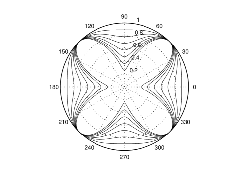
Figure 2: Illustration of the phase penalty function $g^{|\cdot|,\theta}\left(\theta_{\hat{\bar{X}}(k)-\langle\hat{\bar{X}}(k)\rangle}\right)$ expressed in (IV-B). The function is normalized, and therefore the outer circle-shaped curves actually correspond to the smallest magnitudes, and become more tapered as $|\hat{\bar{X}}(k)-\langle\hat{\bar{X}}(k)\rangle|$ increases.

​which is portrayed in Fig. 2 for different magnitudes. The last approximation we wish to mention is the simple magnitude-based function

$$\mathfrak{R}^{|\cdot|}(k)=f_{D(k)}\left(\hat{\bar{X}}(k)-\langle\hat{\bar{X}}(k)\rangle\right)$$ (13)

which is completely blind to the other constellation points. Nonetheless, for small $\sigma_{D}^{2}$ this approximation is very efficient, especially for inner points in large constellations. Once the type of function is set and the vector $\mathfrak{R}$ is computed, we can directly select $\Omega_{m}$ from (8), fix our model (6), and proceed to recovering $c$ by CS.

To be sure, we used two different schemes of CS to recover $c$ from the developed CS model in (6), one from the convex relaxation group and the other from greedy pursuit methods. More specifically, the first is a weighted and phase-augmented LASSO [9] we refer to as WPAL [3], which is a data aided modification of the standard LASSO that incorporates data in the time domain to improve distortion recovery, and can be defined as

$$\hat{c}=\arg_{c}\min\||\textbf{F}^{H}\hat{\bar{X}}-\gamma|^{T}c\|_{1}\,\,\textmd{s.t.}\,\,\|Y^{\prime}_{\Omega_{m}}-\tilde{\Psi}_{\Omega_{m}}c\|_{2}^{2}<\epsilon$$ (14)

for some noise-dependent parameter $\epsilon$. The other technique is the Bayesian Matching Pursuit (BMP) by Schniter et al. [8] chosen for its superior performance and efficiency when a relatively large amount of measurements is available to it, a luxury we can actually enjoy in this work, unlike when pilot reservation is used to construct the observation vector $Y^{\prime}_{\Omega_{m}}$ and an extreme economy in tones is enforced to preserve data rate [3].

V Simulation Results

The methods proposed in this paper were tested on an OFDM signal of $64$ subcarriers drawn from a $16$-QAM constellation. The signal was subject to a block-fading, frequency-selective Rayleigh channel model with an SNR of $25$ dB per bit, and a severe clipping level (defined as $10\log\gamma^{2}/\sigma_{x}^{2}$) of $2$ dB. No bit loading (i.e. no variation of constellation size per carrier SNR), diversity gain, or error control coding were considered. Special packages for convex programming [7], and greedy pursuit [8] were used to implement our CS algorithms.

Fig. 3 shows the result of using WPAL (14) with the proposed reliability criteria in IV for choosing the measurement tone set $\Omega_{m}$. We plotted the results against an increased number of observed tones, such that, for instance, the most $10$ reliable observations are used, compared to using the most $20$ reliable observations, and so on. In doing so we expect a somewhat convex behavior of the SER as a function of $|\Omega_{m}|$, since generally the more observations we use the better the performance of CS algorithms become (up to some typical saturation level), but then due to the increased amount of erroneous observations supplied as $|\Omega_{m}|$ increases, the performance eventually deteriorates. The simulation results confirm this intuition, and also confirm the relative performance of the three methods proposed in (9), (10), and (13), denoted by $\Omega_{m}^{\textmd{Bayes}}$, $\Omega_{m}^{|\cdot|,\theta}$, and $\Omega_{m}^{|\cdot|}$, respectively, as well as the reversed relative performance of the least reliable tone set of each, which we generically denote by $\arg\left\{\mathfrak{R}_{i:N}\right\}_{i=1}^{m}$.

Furthermore, using our practical reliability function (10) based on (IV-B), we compared our results with what we consider the most popular nonlinear distortion mitigation techniques in the literature, namely, the Iterative ML Decoding (ItML)[4] and the Decision-Aided Reconstruction (DAR)[5] techniques. In addition, we also implemented the Quasi-ML technique in [6] which proposed improving the algorithm in [4] by refraining from making hard decisions when the absolute value of the real or imaginary part of the frequency deviation is larger than some linear function $\epsilon$ of $d_{min}$. Results in Fig. 4 show the superior performance of using BMP [8] over the set $\Omega_{m}^{|\cdot|,\theta}$, using only half the tones to reach the optimum performance. The WPAL performs significantly better than Zero Forcing (ZF), and can be used to improve the results of ItML, even though it performs less efficiently alone under most circumstances. Lastly, no gain is achieved by supplying the BMP estimate to ItML, as BMP alone normally outperforms this procedure.

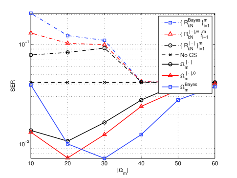
Figure 3: SER vs. $|\Omega_{m}|$ for the various reliability functions defined in (9), (10), and (13) and their least reliable counterparts.

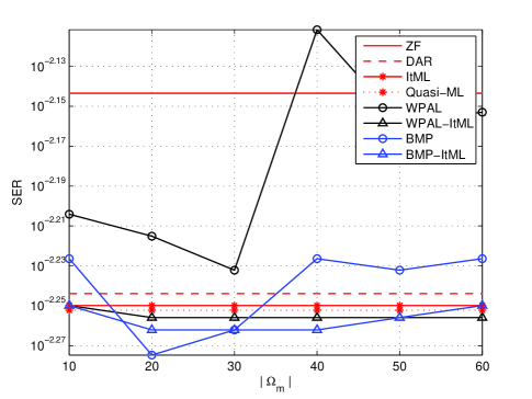
Figure 4: Performance Comparison of CS techniques (alone and over ItML) with ItML [4], DAR [5], and Quasi-ML [6] as a varying amount of the most reliable observations in $\Omega_{m}^{|\cdot|,\theta}$ are considered.

VI Conclusion

A novel method has been proposed to use data-aided CS techniques over a reliable subset of observations in the frequency domain in order to estimate and cancel sparse nonlinear distortion on an OFDM signal in the time domain. Moreover, a newly developed method of computing the reliability of each observation independently of the other $M-1$ candidates within a constellation was also proposed and tested. The methods offer promising performance, and the authors are considering several possible improvements such as invoking soft decoding and CNR maximization.

References

- [1] H. A. David, Order Statistics, Wiley Interscience edition, 1981
- [2] E. B. Al-Safadi and T. Y. Al-Naffouri, “On Reducing the Complexity of Tone Reservation Based PAPR Reduction Schemes by Compressive Sensing,” IEEE Globecom ’09, Honolulu HI, Nov. 2009.
- [3] E. B. Al-Safadi and T. Y. Al-Naffouri, “Peak Reduction and Clipping Mitigation by Compressive Sensing,” IEEE Trans. On Sig. Proc. Available: arXiv:1101.4335v1, submitted for publication
- [4] J. Tellado et. al. “Maximum-Likelihood Detection of Nonlinearly Distorted Multicarrier Symbols by Iterative Decoding,” IEEE Trans. On Comm., vol. 51 no. 2, pp. 218-228, Feb. 2003.
- [5] D. Kim and G.L. Stuber “Clipping Noise Mitigation for OFDM by Decision-Aided Reconstruction,” IEEE Comm. Letters, vol. 3 no. 1, pp. 4-6, Jan. 1999.
- [6] S. Prot et. al. “Conditional Quasi Maximum Likelihood Receiver for Clipped OFDM Signals,” European Conference on Circuit Theory and Design, ECCTD ’05, August 2005.
- [7] M. Grant and S. Boyd. CVX: Matlab software for disciplined convex programming (web page and software). http://stanford.edu/ boyd/cvx, February 2009.
- [8] P. Schniter et. al. “Fast bayesian matching pursuit,” Workshop on Inf. Theory and Applicat. (ITA), La Jolla, CA, Jan. 2008.
- [9] R. Tibshirani, “Regression Shrinkage and Selection via the LASSO,” J. of the Roy. Stat. Soc., Series B, vol. 58, no. 1, pp. 267-288, 1996.