Global phase diagram of two-dimensional Dirac fermions in random potentials

Abstract

Anderson localization is studied for two flavors of massless Dirac fermions in two-dimensional space perturbed by static disorder that is invariant under a chiral symmetry (chS) and a time-reversal symmetry (TRS) operation which, when squared, is equal either to plus or minus the identity. The former TRS (symmetry class BDI) can for example be realized when the Dirac fermions emerge from spinless fermions hopping on a two-dimensional lattice with a linear energy dispersion such as the honeycomb lattice (graphene) or the square lattice with $\pi$-flux per plaquette. The latter TRS is realized by the surface states of three-dimensional $\mathbb{Z}^{\ }_{2}$-topological band insulators in symmetry class CII. In the phase diagram parametrized by the disorder strengths, there is an infrared stable line of critical points for both symmetry classes BDI and CII. Here we discuss a “global phase diagram” in which disordered Dirac fermion systems in all three chiral symmetry classes, AIII, CII, and BDI, occur in 4 quadrants, sharing one corner which represents the clean Dirac fermion limit. This phase diagram also includes symmetry classes AII [e.g., appearing at the surface of a disordered three-dimensional $\mathbb{Z}^{\ }_{2}$-topological band insulator in the spin-orbit (symplectic) symmetry class] and D (e.g., the random bond Ising model in two dimensions) as boundaries separating regions of the phase diagram belonging to the three chS classes AIII, BDI, and CII. Moreover, we argue that physics of Anderson localization in the CII phase can be presented in terms of a non-linear-sigma model (NL$\sigma$M) with a $\mathbb{Z}^{\ }_{2}$-topological term. We thereby complete the derivation of topological or Wess-Zumino-Novikov-Witten terms in the NL$\sigma$M description of disordered fermionic models in all 10 symmetry classes relevant to Anderson localization in two spatial dimensions.

I Introduction

I.1 Dirac fermions in condensed matter physics

Massless Dirac fermions emerge quite naturally from non-interacting and bipartite tight-binding Hamiltonians at low energies and long wave-lengths when the fermion spectrum of energy eigenvalues is symmetric about the band center and the Fermi surface reduces to a finite number of discrete Fermi points at the band center. This situation is generic for non-interacting electrons hopping with a uniform nearest-neighbor amplitude $t$ along a one-dimensional chain. For non-interacting electrons hopping on higher dimensional lattices, this situation is the exception rather than the rule, for it is only fulfilled when the hopping amplitudes are fine-tuned to the lattice.

In the case of graphene, when described by the uniform hopping amplitude $t$ between the nearest-neighbor sites of the honeycomb lattice, there are two bands in the Brillouin zone of the underlying triangular Bravais lattice that touch at the 6 corners of the Brillouin zone [see Fig. 1(a)]. Wallace47 Because the unit cell contains two sites and because the number of inequivalent Fermi points is two, these Dirac fermions realize a four-dimensional representation of the Dirac equation in two-dimensional space if we ignore the spin degrees of freedom.

For non-interacting spinless electrons hopping on the square and (hyper-)cubic lattices, Dirac fermions emerge in the vicinity of the band center whenever the translation invariance of the lattice is broken by choosing the sign of the nearest-neighbor hopping amplitudes of uniform magnitude $t$ in such a way that their products along any elementary closed path (a plaquette) is $-t^{4}$ [see Fig. 1(b)]. This pattern of nearest-neighbor hopping amplitudes preserves time-reversal symmetry. It amounts to threading each plaquette by a magnetic flux of $\pi$ or, equivalently, $-\pi$ in appropriate units and is thus called the $\pi$ flux phase. In the $\pi$-flux phase for the $d$-dimensional hypercubic lattice, there are $2^{d}$ non-equivalent sublattices. Correspondingly there are $2^{d}$ Fermi points and the emerging Dirac Hamiltonian in the vicinity of these Fermi points is $2^{d}$ dimensional. Because the minimal irreducible representation of the Dirac equation in $d$ dimensions is $2^{[(d+1)/2]}$ dimensional ($[x]$ denotes the largest integer smaller than or equal to $x$), the $\pi$-flux phase yields a representation of the Dirac equation larger than the minimal one in all dimensions except for $d=1$. This is called the fermion doubling problem, for it prevents a lattice regularization of the standard model of Elementary Particle Physics that represents its particle content (quarks, leptons).  Wilson75

The fact that the fermion-doubling problem affects both graphene and the $\pi$-flux phase in two dimensions is not a coincidence. The fermion-doubling problem is a generic property of non-interacting local tight-binding Hamiltonians with time-reversal symmetry. Nielsen81

It is possible to circumvent the fermion-doubling problem in the following way.

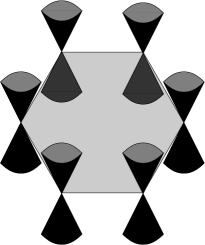
(a) (b)

Figure 1: (a) Hexagonal Brillouin zone of graphene with the conduction and valence bands touching at the zone corners in the linear approximation. There are $6/3=2$ inequivalent Fermi points (Dirac cones). (b) The $\pi$-flux phase for the cubic lattice assigns the nearest-neighbor hopping amplitudes $+t$ for the thin bonds and $-t$ for the thick bonds with $t$ a real number. There are $8=2^{3}$ inequivalent sublattices labeled 1 to 8.

We consider first a one-dimensional chain along which a spinless electron hops with the uniform nearest-neighbor amplitude $t$. We also impose periodic boundary conditions [see Fig. 2(a)]. We fold the spinless electron’s dispersion on half of its Brillouin zone and open a gap at the folded zone boundaries by dimerization of the hopping amplitude, $t\to t\pm\delta t$, as it occurs for example through its interaction with an optical phonon within a Born-Oppenheimer approximation. At low energies, the effective fermionic Hamiltonian is the one-dimensional massive Dirac equation with the mass set by the dimensionless parameter $\delta t/t$ assumed to be smaller than unity. Imagine now that the dimerization pattern is defective at two sites that are far apart relative to the characteristic length scale $(t/\delta t)\mathfrak{a}$ where $\mathfrak{a}$ is the lattice spacing [see Fig. 2(c)]. At the level of the effective Dirac equation, this means that the mass term changes sign twice, once at each defective site. Two bound (i.e., normalizable) states appear in the spectrum [see Fig. 2(d)] with the remarkable property that they have opposite helicity (chirality) and an exponentially small overlap or, equivalently, energy splitting, for they are exponentially localized with the localization length of order $(t/\delta t)\mathfrak{a}$ around their respective defective sites. Jackiw76 ; Su79

The same mechanism applies in any $d$-dimensional space, be it for the massive Dirac equation, Callan85 or for tight-binding Hamiltonians with sublattice symmetry [see Fig. 2(e)], Fradkin86- ; Brouwer02 and has been used in lattice gauge theory as a means to overcome the fermion doubling problem.Kaplan92 ; Jansen96 For example, the massive Dirac equation in odd $d$-dimensional space supports massless boundary states with a common helicity (chirality) along each even $(d-1)$-dimensional boundary where the mass term vanishes. A complete classification of all such two-dimensional boundary states was part of the classification of topological insulators in spatial dimensions $d=1,2,3$ given in Ref. Schnyder08, in terms of the generic symmetry classes arising from the antiunitary operations of time reversal and particle-hole symmetry [underlying the work of Altland and Zirnbauer on random matrix theory (RMT)]. Zirnbauer96 ; Altland97 ; Heinzner05 A systematic regularity (periodicity) of the classification as the dimensionality is varied, in general dimension, was discovered upon the use of K-Theory by Kitaev Kitaev09 (see also Ref. Stone11, ). As shown in Refs. Schnyder09b, and Ryu10b, , this can, alternatively, be understood in terms of the lack of Anderson localization at the boundaries. More recently, an understanding of this classification of topological insulators in terms of quantum anomalies was developed. Ryu11

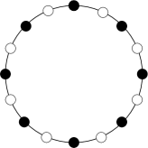
(a) (b)

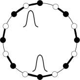
(c) (d)

(e)

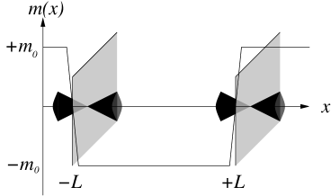
Figure 2: (a) Ring along which a spinless electron hops between nearest-neighbor sites shown as circles with the uniform real-valued amplitude $t$. The lattice sites are colored in black on one sublattice and white on the other sublattice. (b) Electronic dispersion corresponding to (a) after folding the Brillouin zone. (c) Ring along which a spinless electron hops between nearest-neighbor sites with the dimerized real-valued amplitude $t\pm\delta t$. There are two defective sites belonging to opposite sublattices at which two strong bonds $t+\delta t$ meet. (d) The breaking of translation invariance in (c) has opened a gap at the reduced zone boundaries and localized two bound states around the two defective sites. (e) A generalization of (c) and (d) in three dimensions can be achieved with the help of a suitable dimerization of the $\pi$-flux phase depicted in Fig. 1(b) for spinless electrons. The continuum approximation yields a massive $8\times 8$ Dirac equation. Two-dimensional defective surfaces normal to the direction $x$, say, occur when the mass changes sign. One mid-gap state is bound to each of the two-dimensional defective surfaces. Each midgap state obeys a $4\times 4$ two-dimensional massless Dirac equation as depicted by a Dirac cone. The two mid-gap states have opposite chiralities.

Table 1: Table of topological terms that can be added to the replicated fermionic non-linear-sigma model (NL$\sigma$M) describing Anderson localization in two dimensions and the classificationSchnyder08 of topological insulators (superconductors) in three dimensions. Symmetry classes indicated by the “Cartan label” are classified according to the presence or absence of time-reversal, particle-hole, and “sublattice” symmetries which we abbreviate as TRS, PHS, and SLS, respectively. The presence of TRS and PHS is denoted by “$+1$” or “$-1$,” depending on whether the square of the (antiunitary) operator implementing the symmetries equals $+1$ (identity) or $-1$, whereas the presence of SLS is denoted by “1”. The absence of these symmetries is denoted by “0”. The SLS is a product of TRS and PHS. For historical reasons, the first three rows of the table are also referred to as the orthogonal, unitary, and symplectic symmetry classes. When the disorder respects a sublattice symmetry as in the next three rows, the terminology chiral is also used. Finally, the last four rows can be realized as random Bogoliubov-de-Gennes (BdG) Hamiltonians. Target spaces for fermionic replicated NL$\sigma$M ($\mathsf{N}$ is the replica index and the limit $\mathsf{N}\to 0$ is understood) are given in the fifth column. The penultimate column lists the nature of the topological term compatible with the target and two-dimensional base spaces. The symbols $\mathbb{Z}$ and $\mathbb{Z}_{2}$ in the last column indicate that the topologically distinct phases within a given symmetry class of topological insulators or superconductors in three spatial dimensions are characterized by an integer topological invariant ($\mathbb{Z}$) or a $\mathbb{Z}_{2}$ quantity. The symbol “0” denotes the case when there exists no topological insulator (superconductor).

Cartan label	TRS	PHS	SLS	Target space	Topological term	3d-TI/TSC
AI (orthogonal)	$+1$	0	0	$\mathrm{Sp}(4\mathsf{N})/\mathrm{Sp}(2\mathsf{N})\times\mathrm{Sp}(2\mathsf{N})$	–	0
A (unitary)	0	0	0	$\mathrm{U}(2\mathsf{N})/\mathrm{U}(\mathsf{N})\times\mathrm{U}(\mathsf{N})$	$\theta$ term	0
AII (symplectic)	$-1$	0	0	$\mathrm{O}(2\mathsf{N})/\mathrm{O}(\mathsf{N})\times\mathrm{O}(\mathsf{N})$	$\mathbb{Z}^{\ }_{2}$ term	$\mathbb{Z}_{2}$
BDI (chiral orthogonal)	$+1$	$+1$	1	$\mathrm{U}(2\mathsf{N})/\mathrm{Sp}(2\mathsf{N})$	–	0
AIII (chiral unitary)	0	0	1	$\mathrm{U}(\mathsf{N})\times\mathrm{U}(\mathsf{N})/\mathrm{U}(\mathsf{N})$	WZNW term	$\mathbb{Z}$
CII (chiral symplectic)	$-1$	0	1	$\mathrm{U}(\mathsf{N})/\mathrm{O}(\mathsf{N})$	$\mathbb{Z}^{\ }_{2}$ term	$\mathbb{Z}_{2}$
CI (BdG)	$+1$	$-1$	1	$\mathrm{Sp}(2\mathsf{N})\times\mathrm{Sp}(2\mathsf{N})/\mathrm{Sp}(2\mathsf{N})$	WZNW term	$\mathbb{Z}$
C (BdG)	0	$-1$	0	$\mathrm{Sp}(2\mathsf{N})/\mathrm{U}(\mathsf{N})$	$\theta$ term	0
DIII (BdG)	$-1$	$+1$	1	$\mathrm{O}(\mathsf{N})\times\mathrm{O}(\mathsf{N})/\mathrm{O}(\mathsf{N})$	WZNW term	$\mathbb{Z}$
D (BdG)	0	$+1$	0	$\mathrm{O}(2\mathsf{N})/\mathrm{U}(\mathsf{N})$	$\theta$ term	0

I.2 Anderson localization for Dirac fermions in two dimensions

Anderson localization Evers08 for non-interacting two-dimensional Dirac fermions was first studied in narrow gap semiconductors by Fradkin in 1986. Fradkin86 This work was followed up in the 90’s with non-perturbative results motivated by the physics of the integer quantum Hall effect (IQHE), the random bond Ising model, and dirty $d$-wave superconductors.Ludwig94 ; Nersesyan95 ; Chamon96a ; Chamon96b ; Mudry96 ; Bocquet00 ; Bhaseen01 ; Ludwig00 ; Altland02 With the recently available transport measurements in mesoscopic samples of graphene, as well as the identifications of the alloy Bi${}^{\ }_{1-x}$Sb${}^{\ }_{x}$ in a certain range of compositions $x$,Fu07 ; Hsieh08 ; Hsieh09 the compounds Bi${}^{\ }_{2}$Te${}^{\ }_{3}$, Zhang09 ; Chen09 Sb${}^{\ }_{2}$Te${}^{\ }_{3}$, Zhang09 and Bi${}^{\ }_{2}$Se${}^{\ }_{3}$, Zhang09 ; Xia09 and the prediction for another 50 and counting materials as three-dimensional $\mathbb{Z}^{\ }_{2}$-topological band insulators that support surface Dirac fermions, Lin10 ; Yan10 ; Chen10 the localization properties of random Dirac fermions have become relevant from an experimental point of view.

While all these examples share the massless Dirac spectrum as the energy dispersion in the non-interacting and clean limit, the effects induced by randomness – weak localization, universal conductance fluctuations, localization, metal-insulator transition, spectral singularities, etc – vary with (i) the intrinsic symmetries respected by the disorder, (ii) the dimensionality of the Dirac matrices representing the Dirac Hamiltonian, and (iii) the strength and/or correlations in space of the disorder.

When space is effectively zero-dimensional, i.e., at the level of RMT, ten symmetry classes have originally been identified and labeled according to the Cartan classification of symmetric spaces (see Table 1). Zirnbauer96 ; Altland97 ; Heinzner05

As emphasized in Refs. Fendley00, ; Fendley01, , the two-dimensional fermionic replicated NL$\sigma$Ms in eight of the ten symmetry classes allow for terms of topological origin, in the form of either $\theta$ terms theta-term or Wess-Zumino-Novikov-Witten (WZNW) terms Wess71 ; Novikov82 ; Witten84 (see Table 1). Symmetry classes A, C, and D support Pruisken ($\theta$) terms.Pruisken84 ; Senthil98 ; Senthil00 Symmetry classes AIII, DIII, and CI support WZNW terms. Finally, symmetry classes AII and CII support $\mathbb{Z}^{\ }_{2}$-topological terms.

WZNW terms in symmetry classes AIII, DIII, and CI appear when Dirac fermions propagate in the presence of static vector-gauge-like randomness. Ludwig94 ; Nersesyan95 ; Chamon96a ; Chamon96b ; Mudry96 ; Mudry99 ; Bocquet00 ; Bhaseen01 ; Ludwig00 ; Altland02 This can only be achieved at the lattice level if the fermion doubling problem has been overcome, as is the case with the surface states of three-dimensional $\mathbb{Z}$-topological band insulators.

The $\mathbb{Z}^{\ }_{2}$-topological term in symmetry class AII was derived in the context of disordered graphene with long-range correlated disorder Ostrovsky07 ; Ryu07b or two-dimensional surfaces of three-dimensional $\mathbb{Z}^{\ }_{2}$ topological band insulators. Ryu07b

LeClair and Bernard have extended the RMT classification by demanding that all perturbations to the two-dimensional Dirac Hamiltonian with $\mathrm{N}^{\ }_{\mathrm{f}}$ flavors preserve the Dirac structure.Bernard02 In this way, the ten-fold classification can be refined by discriminating the parity of $\mathrm{N}^{\ }_{\mathrm{f}}$ for the 3 symmetry classes AIII, DIII, and CI. These 3 subclasses correspond to the fact that the replicated principal chiral models (PCMs) whose target space correspond to symmetry classes AIII, DIII, and CI, respectively, can be augmented by WZNW terms. The realization of any of these additional 3 subclasses in a lattice model requires overcoming the fermion doubling problem.

The parity of the flavor number $\mathrm{N}^{\ }_{\mathrm{f}}$ of random Dirac fermions also matters for symmetry classes AII and CII. The fermionic replicated NL$\sigma$Ms derived from the random Dirac Hamiltonians in symmetry classes AII and CII can acquire a $\mathbb{Z}^{\ }_{2}$ topological term on account of the dimensionality of the Dirac matrices (twice the number $\mathrm{N}^{\ }_{\mathrm{f}}$ of flavors) that represents the random Dirac Hamiltonian. Deriving these $\mathbb{Z}^{\ }_{2}$ topological terms from lattice models is not automatic, for the fermion doubling problem must be surmounted.

In this paper, by identifying a disordered fermionic model that gives rise to the $\mathbb{Z}^{\ }_{2}$-topological term in symmetry class CII, we complete the derivation for non-interacting fermions subject to a weak white-noise correlated random potential of topological or WZNW terms in all 10 symmetry classes relevant to two-dimensional Anderson localization. The microscopic fermionic model is realized by the surface states of a three-dimensional $\mathbb{Z}^{\ }_{2}$ topological band insulator in symmetry class CII of Ref. Schnyder08, . (See Ref. Hosur2010, for a particular lattice model of a three-dimensional $\mathbb{Z}_{2}$ topological insulator in symmetry class CII.)

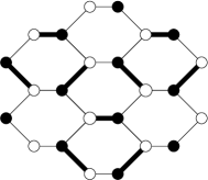
(a) (b)

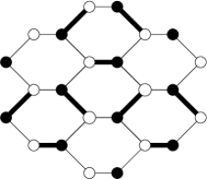
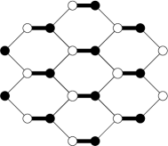
(c) (d)

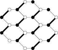
Figure 3: The four independent dimerization patterns for the real-valued nearest-neighbor hopping amplitudes of a spinless electron on the honeycomb lattice that preserve the sublattice symmetry and the time-reversal symmetry for a spinless particle. The two triangular sublattices of the honeycomb lattice are distinguished by the coloring of their sites (white or black colored circles). Strong and weak bonds are depicted by thick and thin lines, respectively. The two independent Kékule dimerization patterns (a) and (b) are responsible for the opening of a complex-valued gap $m$ in the continuum approximation by a $4\times 4$ Dirac equation. The two independent columnar dimerization patterns (c) and (d) are responsible for the emergence of an axial vector gauge field or, equivalently, the complex-valued axial gauge field $a^{\prime}$ in the continuum approximation by a $4\times 4$ Dirac equation.

I.3 Global phase diagram

In this paper, we start from the kinetic Hamiltonian $\mathcal{K}$ for $\mathrm{N}^{\ }_{\mathrm{f}}=2$ flavors of Dirac fermions that make up a (reducible) 4-dimensional representation of the homogeneous Lorentz group $\mathrm{SO}(1,2)$. We then subject $\mathcal{K}$ to a static and chiral-symmetric random potential $\mathcal{V}$, i.e., the random Dirac Hamiltonian $\mathcal{H}=\mathcal{K}+\mathcal{V}$ must anticommute with a unitary matrix $\mathcal{C}$, $\left\{\mathcal{H},\mathcal{C}\right\}=0$, which squares to the identity. By imposing the condition that $\mathcal{H}$ is invariant under a representation $\mathcal{T}=\mathcal{T}^{T}$ of time reversal for spinless single-particle states, $\mathcal{H}$ belongs to symmetry class BDI in the 10-fold classification (see Table 1). This corresponds to an antiunitary time reversal operator whose square equals plus the identity.

It is also known that such a Hamiltonian $\mathcal{H}$ describes graphene (see Fig. 3) or the two-dimensional $\pi$-flux phase, in the presence of real-valued, nearest-neighbor, spin-independent, random hopping amplitudes when the Fermi energy is at the band center and once the long-wave-length limit has been taken with respect to the discrete Fermi points.Hatsugai97 ; Guruswamy00 ; Mudry03 ; Ostrovsky06 ; Ryu07a ; Ryu10a For the case of graphene, CastroNeto08 static random real-valued nearest-neighbor hopping amplitudes are induced by neglecting Lee73 the dynamics of phonons relative to that of the electrons to which they couple. We emphasize that it is imperative to treat all channels (see Fig. 3) of disorder compatible with the chiral and time-reversal symmetries.

The first result of this paper is that analytical continuation of the real-valued random hopping amplitudes to imaginary ones in the aforementioned bipartite lattice models yields a random Dirac Hamiltonian that belongs to symmetry class CII, as it now turns out to obey the time-reversal symmetry (TRS) generated by an operator $\mathcal{T}^{\prime}=-\mathcal{T}^{\prime T}$ acting on an isospin-1/2 single-particle state. This corresponds to an antiunitary time reversal operator whose square equals minus the identity.

Second, we argue that, this random Dirac Hamiltonian captures the (nearly) critical localization properties of the surface states of a lattice model that, in the clean limit, realizes a three-dimensional $\mathbb{Z}^{\ }_{2}$-topological band insulator in symmetry class CII.

More specifically, we show that the phase diagram depicted in Fig. 4 encodes the localization properties of the random Dirac Hamiltonian $\mathcal{H}=\mathcal{K}+\mathcal{V}$ when the chiral-symmetric random potential $\mathcal{V}$ is assigned the three possible independent disorder strengths $g^{\ }_{\mathrm{Re}\,m},g^{\ }_{\mathrm{Im}\,m},g^{\ }_{a^{\prime}}$ which are not irrelevant under the RG. Here we discuss a “global phase diagram”, depicted in Fig. 4(a), in the space of these three couplings which is projected onto the $g^{\ }_{\mathrm{Re}\,m}$ - $g^{\ }_{\mathrm{Im}\,m}$ plane (with $g^{\ }_{a^{\prime}}=0$). In this phase diagram, disordered Dirac fermion systems in all three chiral symmetry classes, AIII, CII, and BDI occur in 4 quadrants, sharing one corner which represents the clean Dirac fermion limit. Also realized in the phase diagram are the symmetry classes AII and D at the boundaries separating the three chiral symmetry classes, whereby the parametrization of class D turns out to follow from analytic continuation of the relevant disorder strength that parametrizes class AII in the phase diagram.

The random Dirac Hamiltonian $\mathcal{H}$ whose potential $\mathcal{V}$ is restricted to symmetry class AII captures the transport properties at long wave lengths of the surface states of a disordered three-dimensional $\mathbb{Z}^{\ }_{2}$-topological band insulator in symmetry class AII (say, Bi${}^{\ }_{1-x}$Sb${}^{\ }_{x}$).Schnyder08

The random Dirac Hamiltonian $\mathcal{H}$ whose potential $\mathcal{V}$ is restricted to symmetry class D captures the transport properties of the fermionic quasiparticles of a disordered two-dimensional chiral $p$-wave superconductor (say, Sr${}^{\ }_{2}$RuO${}^{\ }_{4}$) or their counterparts in the random bond Ising model at long wave lengths.

Figure 4: Global phase diagram for random Dirac fermion defined by Eqs. (12), (13), (14), (23), and (29). (a) Flows of the coupling constants close to the clean Dirac point (the origin denoted by an open circle). Along the boundaries D and AII, the coupling constant $g^{\ }_{a^{\prime}}$ is not generated under the RG, so $g^{\ }_{a^{\prime}}=0$ can be imposed in a consistent way. In fact, symmetry classes D and AII requireSchnyder08 ; Bernard02 $g^{\ }_{a^{\prime}}=0$. Away from these boundaries, $g^{\ }_{a^{\prime}}$ grows under the RG and we have projected the flows onto the $g^{\ }_{a^{\prime}}=0$ plane in the regime where $g^{\ }_{a^{\prime}}$ is still small. In the region denoted BDI of the phase diagram, there exists a line of (nearly) critical points denoted by a dashed line as a result of Eq. (59b). This line of (nearly) critical points is perturbatively stable under the RG flow (63). In the region denoted CII of the phase diagram, there exists a line of (nearly) critical points denoted by a dashed line as a result of Eq. (62b). This line of (nearly) critical points appears to be perturbatively unstable under the RG flow (65) for small values of $g^{\ }_{a^{\prime}}$. (b) Infrared flows dictated by Eq. (63) close to the clean Dirac point when $g^{\ }_{a^{\prime}}>0$. The slopes of the flows on the BDI boundaries $g^{\ }_{\mathrm{Im}\,m}\,g^{\ }_{\mathrm{Re}\,m}=0$ have changed as compared to the case when $g^{\ }_{a^{\prime}}=0$. (c) Infrared flows dictated by Eq. (65) close to the clean Dirac point when $g^{\ }_{a^{\prime}}>g^{\prime}_{+}$ with $g^{\prime}_{\pm}:=g^{\ }_{\mathrm{Im}\,m^{\prime}}\pm g^{\ }_{\mathrm{Re}\,m^{\prime}}$ and $g^{\prime}_{+}\geq|g^{\prime}_{-}|$. The slopes of the flows on the CII boundaries $g^{\prime}_{\mathrm{Im}\,m}\,g^{\prime}_{\mathrm{Re}\,m}=0$ have changed as compared to the case when $g^{\ }_{a^{\prime}}=0$. Moreover, because of the condition $g^{\ }_{a^{\prime}}>g^{\prime}_{+}$, the RG flows in the quadrant CII are towards the surface defined by the dashed line of (nearly) critical points (the $g^{\prime}_{+}$ axis) and the out-of-plane $g^{\ }_{a^{\prime}}$ axis. The plane $g^{\ }_{\mathrm{Im}\,m^{\prime}}$ - $g^{\ }_{a^{\prime}}$ with $g^{\ }_{\mathrm{Re}\,m^{\prime}}=0$ and $g^{\ }_{a^{\prime}}>0$ and the plane $g^{\ }_{\mathrm{Re}\,m^{\prime}}$ - $g^{\ }_{a^{\prime}}$ with $g^{\ }_{\mathrm{Im}\,m^{\prime}}=0$ and $g^{\ }_{a^{\prime}}>0$ are always unstable under the one-loop flow (65). (d) Infrared RG flows of Eq. (65) in the surface defined by the $g^{\prime}_{-}$ axis as horizontal axis and the $g^{\ }_{a^{\prime}}$ axis as vertical axis of the quadrant CII.

Located in the center of the phase diagram of Fig. 4(a) is a vertical dashed line. There exists a sector of the theory that decouplesGuruswamy00 from the random $\mathrm{U}(1)$ gauge potential. This sector is critical along the dashed line in Fig. 4(a). We will call the dashed line in Fig. 4(a) a line of nearly-critical points to account for the non-critical sector that is not depicted in Fig. 4(a).

It is argued in Sec. IV that along the dashed line in region CII of Fig. 4(a), the transport properties of $\mathcal{H}$ are also encoded by those of a NL$\sigma$M on the target manifold appropriate for this symmetry class. (Such a possibility was also discussed, independently and from a different perspective, in Refs. Mitev08, , Candu09, , Candu10, , and Candu11, .) Remarkably, the standard kinetic energy of the NL$\sigma$M must be augmented by a $\mathbb{Z}^{\ }_{2}$-topological term (see Appendix A). Here, the necessary requirement for the presence of the $\mathbb{Z}^{\ }_{2}$-topological term is that the number $\mathrm{N}^{\ }_{\mathrm{f}}$ of flavors be two times an odd integer $n$, i.e. $\mathrm{N}^{\ }_{\mathrm{f}}=2n$. However, any purely two-dimensional non-interacting local tight-binding Hamiltonian with Fermi points at the band center that breaks the spin-rotation symmetry but preserves the time-reversal and sublattice symmetries yields a Dirac equation with $\mathrm{N}^{\ }_{\mathrm{f}}=2n$ where $n$ is an even integer because of the fermion doubling problem. The fermion doubling problem for fermions in two dimensions can be circumvented by working with fermions localized at the two-dimensional boundary of a three-dimensional crystal, i.e., with the boundary states of a topological band insulator in symmetry class CII. It is the nearly-critical localization properties of these surface states that are captured by the dashed line in region CII of Fig. 4. Thus, we can view the $\mathbb{Z}^{\ }_{2}$-topological term in the NL$\sigma$M for symmetry class CII as the signature of the physics of (de)localization, that arises from the existence of boundary states in the clean limit, the defining property of three-dimensional $\mathbb{Z}^{\ }_{2}$-topological band insulators in symmetry class CII.

Third, we argue that the initial flow away from the apparently unstable nearly-critical line in region CII depicted in Fig. 4(a) is not a crossover flow to the diffusive metallic fixed point of the NL$\sigma$M in symmetry class AII augmented by a $\mathbb{Z}^{\ }_{2}$ topological term. Rather, it is the flow depicted in Fig. 4(c) that bends back towards the nearly-critical plane defined by the dashed line and the out-of-plane axis for the coupling $g^{\ }_{a^{\prime}}$ as a result of the RG flow of the coupling $g^{\ }_{a^{\prime}}$ to strong-coupling. This flow on sufficiently large length scales along trajectories in the three-dimensional coupling space is depicted through the two-dimensional cuts presented in Figs. 4(b), 4(c), and 4(d). The full RG flow along the boundary AII, a separatrix of the RG flow, was computed numerically in Refs. Bardarson07, and Nomura07, owing to the presence of a $\mathbb{Z}^{\ }_{2}$-topological term on the target manifold of the NL$\sigma$M appropriate for symmetry class AII.Ostrovsky07 ; Ryu07b

Finally, in the quadrant labeled by BDI, the dashed line also represents a line of nearly-critical points.Hatsugai97 ; Guruswamy00 ; Mudry03 ; Ostrovsky06 ; Ryu10a This line of nearly-critical points is stable, without the reentrant behavior of the kind mentioned in the preceding paragraph. The one-loop RG flow along the boundary D, again a separatrix of the RG flow, was computed in Refs. Dotsenko83, , Ludwig87, , and Shankar87, .

The fact that the quadrant in symmetry class BDI can be analytically continued to the quadrant in symmetry class CII suggests that one can compute properties of the latter phase from the former one. In particular, sets of non-perturbative and exact results have been obtained for e.g., boundary multifractal exponents for the point contact conductance on the critical line in symmetry class BDI. Obuse08 ; Quella08 These results will also apply to the critical line in symmetry class CII upon suitable analytical continuation.

I.4 Outline

The rest of the paper is organized as follows: The non-interacting random Dirac fermion model is defined in Sec. II. The main result of this section is captured by Fig. 4. We argue in Secs. III and IV that the generating function for the moments of the retarded Green’s functions for microscopic parameters corresponding to the quadrant CII in Fig. 4 realizes a replicated fermionic or, alternatively, a supersymmetric (SUSY) NL$\sigma$M augmented by a $\mathbb{Z}^{\ }_{2}$-topological term. We conclude in Sec. V.

II Definitions and phase diagram

We begin in Sec. II.1 by defining a non-interacting random Dirac Hamiltonian and proceed with a symmetry analysis. To identify the axis of the phase diagram in Fig. 4, a generating function for the disorder average over products of $\mathrm{N}$ retarded single-particle Green’s functions is needed. This is done using the supersymmetric (SUSY) formalism in Secs. II.2 and II.3. The flows in Fig. 4 to or away from the nearly-critical line follow once it is shown in Sec. II.4 that the SUSY generating function defines a $\widehat{\mathrm{gl}}(2\mathrm{N}|2\mathrm{N})^{\ }_{k=1}$ SUSY Thirring model studied in Refs. Guruswamy00, and Mudry03, .

II.1 Definitions

Common to all the aforementioned microscopic examples is the existence of 4 Fermi points at the relevant Fermi energy around which linearization in momentum space yields the continuum Dirac kinetic energy

$$\begin{split}\mathcal{K}(\bm{p}):=&\,\begin{pmatrix}0&0&0&p\\ 0&0&\bar{p}&0\\ 0&p&0&0\\ \bar{p}&0&0&0\end{pmatrix}\\ \equiv&\,\begin{pmatrix}0&\sigma^{\ }_{x}p^{\ }_{x}+\sigma^{\ }_{y}p^{\ }_{y}\\ \sigma^{\ }_{x}p^{\ }_{x}+\sigma^{\ }_{y}p^{\ }_{y}&0\end{pmatrix}\\ \equiv&\,\rho^{\ }_{1}\otimes\sigma^{\ }_{1}\,p^{\ }_{1}+\rho^{\ }_{1}\otimes\sigma^{\ }_{2}\,p^{\ }_{2},\end{split}$$ (1)

up to a unitary transformation. Here, the momentum $\bm{p}=(p^{\ }_{x},p^{\ }_{y})\equiv(p^{\ }_{1},p^{\ }_{2})$ is measured relative to the Fermi points at the band center. The complex notation $p=p^{\ }_{x}-{i}p^{\ }_{y}$ and $\bar{p}=p^{\ }_{x}+{i}p^{\ }_{y}$ is occasionally used for conciseness. The unit $2\times 2$ matrix $\sigma^{\ }_{0}$ and the three Pauli matrices $(\sigma^{\ }_{1},\sigma^{\ }_{2},\sigma^{\ }_{3})$ are reserved for the spinor indices of $\mathrm{SO}(1,2)$. The unit $2\times 2$ matrix $\rho^{\ }_{0}$ and the three Pauli matrices $(\rho^{\ }_{1},\rho^{\ }_{2},\rho^{\ }_{3})$ are reserved for the two-dimensional flavor subspace.

This kinetic energy has two interesting properties. First, it anticommutes with the $4\times 4$ unitary and Hermitian matrices

$$\begin{split}&\mathcal{C}^{\ }_{1}:=\rho^{\ }_{3}\otimes\sigma^{\ }_{0},\qquad\mathcal{C}^{\ }_{1}\mathcal{C}^{{\dagger}}_{1}=\mathcal{C}^{\ }_{1}\mathcal{C}^{\ }_{1}=+\mathcal{C}^{\ }_{1}\mathcal{C}^{*}_{1}=1,\\ &\mathcal{C}^{\ }_{2}:=\rho^{\ }_{2}\otimes\sigma^{\ }_{0},\qquad\mathcal{C}^{\ }_{2}\mathcal{C}^{{\dagger}}_{2}=\mathcal{C}^{\ }_{2}\mathcal{C}^{\ }_{2}=-\mathcal{C}^{\ }_{2}\mathcal{C}^{*}_{2}=1,\\ &\mathcal{C}^{\ }_{3}:=\rho^{\ }_{0}\otimes\sigma^{\ }_{3},\qquad\mathcal{C}^{\ }_{3}\mathcal{C}^{{\dagger}}_{3}=\mathcal{C}^{\ }_{3}\mathcal{C}^{\ }_{3}=+\mathcal{C}^{\ }_{3}\mathcal{C}^{*}_{3}=1,\\ &\mathcal{C}^{\ }_{4}:=\rho^{\ }_{1}\otimes\sigma^{\ }_{3},\qquad\mathcal{C}^{\ }_{4}\mathcal{C}^{{\dagger}}_{4}=\mathcal{C}^{\ }_{4}\mathcal{C}^{\ }_{4}=+\mathcal{C}^{\ }_{4}\mathcal{C}^{*}_{4}=1.\end{split}$$ (2)

Second, the operations on $\mathcal{K}$ consisting in the momentum inversion $\bm{p}\to-\bm{p}$, complex conjugation, and matrix multiplication from the left and from the right by the $4\times 4$ unitary and Hermitian matrices

$$\begin{split}&\mathcal{T}^{\ }_{1}:=\rho^{\ }_{3}\otimes\sigma^{\ }_{1},\qquad\mathcal{T}^{\ }_{1}\mathcal{T}^{{\dagger}}_{1}=\mathcal{T}^{\ }_{1}\mathcal{T}^{\ }_{1}=+\mathcal{T}^{\ }_{1}\mathcal{T}^{*}_{1}=1,\\ &\mathcal{T}^{\ }_{2}:=\rho^{\ }_{0}\otimes\sigma^{\ }_{2},\qquad\mathcal{T}^{\ }_{2}\mathcal{T}^{{\dagger}}_{2}=\mathcal{T}^{\ }_{2}\mathcal{T}^{\ }_{2}=-\mathcal{T}^{\ }_{2}\mathcal{T}^{*}_{2}=1,\\ &\mathcal{T}^{\ }_{3}:=\rho^{\ }_{1}\otimes\sigma^{\ }_{2},\qquad\mathcal{T}^{\ }_{3}\mathcal{T}^{{\dagger}}_{3}=\mathcal{T}^{\ }_{3}\mathcal{T}^{\ }_{3}=-\mathcal{T}^{\ }_{3}\mathcal{T}^{*}_{3}=1,\\ &\mathcal{T}^{\ }_{4}:=\rho^{\ }_{2}\otimes\sigma^{\ }_{1},\qquad\mathcal{T}^{\ }_{4}\mathcal{T}^{{\dagger}}_{4}=\mathcal{T}^{\ }_{4}\mathcal{T}^{\ }_{4}=-\mathcal{T}^{\ }_{4}\mathcal{T}^{*}_{4}=1,\end{split}$$ (3)

all yield $\mathcal{K}$ again. For any $i,j=1,\cdots,4$, the property

$$\mathcal{C}^{\ }_{i}\,\mathcal{K}(\bm{p})\,\mathcal{C}^{\ }_{i}=-\mathcal{K}(\bm{p}),$$ (4)

that we will call (abusively) chiral symmetry (chS), is compatible with the property

$$\mathcal{T}^{\ }_{j}\,\mathcal{K}^{*}(-\bm{p})\,\mathcal{T}^{\ }_{j}=\mathcal{K}(\bm{p}),$$ (5)

that we will call TRS, if and only if

$$[\mathcal{C}^{\ }_{i},\mathcal{T}^{\ }_{j}]=0.$$ (6)

In this paper, we shall assume that the lattice model from which $\mathcal{K}(\bm{p})$ emerges imposes the chiral symmetry generated by

$$\mathcal{C}\equiv\mathcal{C}^{\ }_{1}.$$ (7)

This chiral symmetry commutes with

$$\mathcal{T}\equiv\mathcal{T}^{\ }_{1}$$ (8)

and with

$$\mathcal{T}^{\prime}\equiv\mathcal{T}^{\ }_{2}.$$ (9)

(Observe that $\mathcal{T}$ and $\mathcal{T}^{\prime}$ anticommute. They are not compatible.) This leads to two possible forms of TRS, either the one appropriate for particles with integer isospin when

$$\mathcal{T}^{T}=+\mathcal{T}$$ (10)

is imposed as a symmetry, or the one for particles with half-integer isospin when

$$\mathcal{T}^{\prime T}=-\mathcal{T}^{\prime}$$ (11)

is imposed as a symmetry. Again, the choice between $\mathcal{T}$ and $\mathcal{T}^{\prime}$ is dictated by the underlying lattice model.

The most general static random potential that anticommutes with $\mathcal{C}$ is of the form

$$\begin{split}&\mathcal{V}=\begin{pmatrix}0&V\\ V^{{\dagger}}&0\end{pmatrix},\\ &V=\sigma^{\ }_{1}A^{\ }_{1}+\sigma^{\ }_{2}A^{\ }_{2}+\sigma^{\ }_{3}M^{\ }_{3}+\sigma^{\ }_{0}M^{\ }_{0},\end{split}$$ (12a)

where the complex-valued

$$\begin{split}&A^{\ }_{1}=a^{\ }_{1}-ia^{\prime}_{1},\\ &A^{\ }_{2}=a^{\ }_{2}-ia^{\prime}_{2},\\ &M^{\ }_{3}=-m^{\ }_{3}-im^{\prime}_{3},\\ &M^{\ }_{0}=m^{\prime}_{0}-im^{\ }_{0},\end{split}$$ (12b)

represent sources of (static) randomness, i.e., complex-valued functions of the space coordinates $$\bm{r}\in\mathbb{R}^{2}$$. (The unusual sign conventions is chosen to make contact with the notation of Ref. Mudry03, .) It yields the random Dirac Hamiltonian

$$\begin{split}\mathcal{H}(\bm{r}):=&\,\left(\mathcal{K}+\mathcal{V}\right)(\bm{r})\\ =&\,\left(\begin{array}[]{cc}0&D(\bm{r})\\ D^{{\dagger}}(\bm{r})&0\end{array}\right)\\ =&\,-i\rho^{\ }_{1}\otimes\sigma^{\ }_{1}\,\partial^{\ }_{1}-i\rho^{\ }_{1}\otimes\sigma^{\ }_{2}\,\partial^{\ }_{2}\\ &\,+\rho^{\ }_{1}\otimes\sigma^{\ }_{1}\,a^{\ }_{1}(\bm{r})+\rho^{\ }_{1}\otimes\sigma^{\ }_{2}\,a^{\ }_{2}(\bm{r})\\ &\,+\rho^{\ }_{2}\otimes\sigma^{\ }_{1}\,a^{\prime}_{1}(\bm{r})+\rho^{\ }_{2}\otimes\sigma^{\ }_{2}\,a^{\prime}_{2}(\bm{r})\\ &\,-\rho^{\ }_{1}\otimes\sigma^{\ }_{3}\,m^{\ }_{3}(\bm{r})+\rho^{\ }_{1}\otimes\sigma^{\ }_{0}\,m^{\prime}_{0}(\bm{r})\\ &\,+\rho^{\ }_{2}\otimes\sigma^{\ }_{3}\,m^{\prime}_{3}(\bm{r})+\rho^{\ }_{2}\otimes\sigma^{\ }_{0}\,m^{\ }_{0}(\bm{r}).\end{split}$$ (12c)

By construction, Hamiltonian (12c) is a member of the AIII symmetry class (chiral-unitary symmetry class) of Anderson localization in two dimensions.

When the disorder (12b) is restricted to

$$A^{\ }_{\mu}=-{i}a^{\prime}_{\mu}\in{i}\mathbb{R},\ M^{\ }_{3}=-m^{\ }_{3}\in\mathbb{R},\ M^{\ }_{0}=-{i}m^{\ }_{0}\in{i}\mathbb{R},$$ (13a)

the random Hamiltonian (12c) reduces to

$$\begin{split}\mathcal{H}(\bm{r})=&\,-i\rho^{\ }_{1}\otimes\sigma^{\ }_{1}\,\partial^{\ }_{1}-i\rho^{\ }_{1}\otimes\sigma^{\ }_{2}\,\partial^{\ }_{2}\\ &\,+\rho^{\ }_{2}\otimes\sigma^{\ }_{1}\,a^{\prime}_{1}(\bm{r})+\rho^{\ }_{2}\otimes\sigma^{\ }_{2}\,a^{\prime}_{2}(\bm{r})\\ &\,-\rho^{\ }_{1}\otimes\sigma^{\ }_{3}\,m^{\ }_{3}(\bm{r})+\rho^{\ }_{2}\otimes\sigma^{\ }_{0}\,m^{\ }_{0}(\bm{r})\end{split}$$ (13b)

and hence is invariant under the time-reversal

$$\mathcal{T}\mathcal{H}^{*}(\bm{r})\mathcal{T}=\mathcal{H}(\bm{r}),\qquad\mathcal{T}:=\rho^{\ }_{3}\otimes\sigma^{\ }_{1},$$ (13c)

for any realization of the disorder (13a). Accordingly, this Hamiltonian is a member of the BDI symmetry class (chiral-orthogonal symmetry class) in Anderson localization.

On the other hand, when the disorder (12b) is restricted to

$$A^{\ }_{\mu}=-{i}a^{\prime}_{\mu}\in{i}\mathbb{R},\ M^{\ }_{3}=-{i}m^{\prime}_{3}\in{i}\mathbb{R},\ M^{\ }_{0}=m^{\prime}_{0}\in\mathbb{R},$$ (14a)

the random Hamiltonian (12c) reduces to

$$\begin{split}\mathcal{H}(\bm{r})=&\,-i\rho^{\ }_{1}\otimes\sigma^{\ }_{1}\,\partial^{\ }_{1}-i\rho^{\ }_{1}\otimes\sigma^{\ }_{2}\,\partial^{\ }_{2}\\ &\,+\rho^{\ }_{2}\otimes\sigma^{\ }_{1}\,a^{\prime}_{1}(\bm{r})+\rho^{\ }_{2}\otimes\sigma^{\ }_{2}\,a^{\prime}_{2}(\bm{r})\\ &\,+\rho^{\ }_{2}\otimes\sigma^{\ }_{3}\,m^{\prime}_{3}(\bm{r})+\rho^{\ }_{1}\otimes\sigma^{\ }_{0}\,m^{\prime}_{0}(\bm{r})\end{split}$$ (14b)

and hence is invariant under the time-reversal

$$\mathcal{T}^{\prime}\mathcal{H}^{*}(\bm{r})\mathcal{T}^{\prime}=\mathcal{H}(\bm{r}),\qquad\mathcal{T}^{\prime}:=\rho^{\ }_{0}\otimes\sigma^{\ }_{2},$$ (14c)

for any realization of the disorder (14a). Accordingly, this Hamiltonian is a member of the CII symmetry class (chiral-symplectic symmetry class) in Anderson localization.

The BDI case (13) can be derived as the continuum limit of a real-valued, nearest-neighbor, spin-independent, and random hopping model on a bipartite lattice; the honeycomb lattice of graphene or the square lattice with a $\pi$-flux phase say.Hatsugai97 The four-dimensional subspace associated to the $\rho$’s and $\sigma$’s originates from the 2-sublattices structure and the 2 non-equivalent Fermi points at the band center. The electronic spin plays here no role besides an overall degeneracy factor as spin-orbit coupling is neglected. In the context of graphene, the random fields $a^{\prime}_{1}$ and $a^{\prime}_{2}$ are called ripples [see Fig. 3(c-d)],ripples while the random masses $m^{\ }_{3}$ and $m^{\ }_{0}$ are smooth bond fluctuations about the Kekulé dimerization pattern of the nearest-neighbor hopping amplitude [see Fig. 3(a-b)]. Hou07 In the context of the $\pi$-flux phase, the random fields $a^{\prime}_{1}$ and $a^{\prime}_{2}$ are smooth fluctuations of the nearest-neighbor hopping amplitudes about the two wave vectors for the two independent staggered dimerization patterns, while the random masses $m^{\ }_{3}$ and $m^{\ }_{0}$ are smooth bond fluctuations about the two independent columnar dimerization pattern. Fradkin91 The CII case (14) can be derived as the restriction to a two-dimensional boundary of a disordered, three-dimensional $\mathbb{Z}^{\ }_{2}$-topological band insulator in the chiral-symplectic class of Anderson localization. Schnyder08

When the disorder is restricted to

$$A^{\ }_{\mu}=0,\qquad M^{\ }_{3}=-m^{\ }_{3}\in\mathbb{R},\qquad M^{\ }_{0}=0,$$ (15a)

we observe that Hamiltonian (12c) reduces to

$$\mathcal{H}=\rho^{\ }_{1}\otimes D,$$ (15b)

with

$$D=D^{\dagger},\qquad\sigma_{1}D^{*}\sigma_{1}=-D,$$ (15c)

and can be thought of as a random Hamiltonian belonging to the symmetry class D (BdG Hamiltonians with both time-reversal symmetry and spin-1/2 rotation symmetry broken) in Anderson localization, for $$\mathcal{H}$$ is then unitarily equivalent to

$$\left(\begin{array}[]{cc}D&0\\ 0&-D\end{array}\right)$$ (15d)

with the unitary transformation $(\rho^{\ }_{0}+i\rho^{\ }_{2})\otimes\sigma^{\ }_{0}/\sqrt{2}$.

Finally, when the disorder is restricted to

$$A^{\ }_{\mu}=0,\qquad M^{\ }_{3}=0,\qquad M^{\ }_{0}=m^{\prime}_{0}\in\mathbb{R},$$ (16a)

we observe that Hamiltonian (12c) reduces to

$$\mathcal{H}=\rho^{\ }_{1}\otimes D$$ (16b)

with

$$D=D^{\dagger},\qquad\sigma^{\ }_{2}D^{*}\sigma^{\ }_{2}=D,$$ (16c)

and can be thought of as a random Hamiltonian belonging to symmetry class AII (a spin-$1/2$ electron with time-reversal symmetry but without spin-rotation symmetry) in Anderson localization, for $\mathcal{H}$ can then be brought to the block diagonal form (15d) by the same unitary transformation used to reach (15d).

All four symmetry conditions are summarized in Table 2. The defining conditions on classes D and AII can be made slightly more general than in Eqs. (15a) and (16a) as will become clear at the end of Sec. II.3.

Table 2: Symmetry conditions on the static random fields in the Hamiltonian (12). For the symmetry classes D and AII, $M^{\ }_{3}M^{\ }_{0}=0$ must hold.

	AIII	BDI	CII	D	AII
$A^{\ }_{1}$	$a^{\ }_{1}-{i}a^{\prime}_{1}$	$-{i}a^{\prime}_{1}$	$-{i}a^{\prime}_{1}$	$0$	$0$
$A^{\ }_{2}$	$a^{\ }_{2}-{i}a^{\prime}_{2}$	$-{i}a^{\prime}_{2}$	$-{i}a^{\prime}_{2}$	$0$	$0$
$M^{\ }_{3}$	$-m^{\ }_{3}-{i}m^{\prime}_{3}$	$-m^{\ }_{3}$	$-{i}m^{\prime}_{3}$	$-m^{\ }_{3}$	$-{i}m^{\prime}_{3}$
$M^{\ }_{0}$	$m^{\prime}_{0}-{i}m^{\ }_{0}$	$-{i}m^{\ }_{0}$	$m^{\prime}_{0}$	$-{i}m^{\ }_{0}$	$m^{\prime}_{0}$

II.2 Path integral representation of the single-particle Green’s function

In Anderson localization, physical quantities are expressed by (products of) the retarded ($+{i}\eta$, $\eta>0$) and advanced ($-{i}\eta$) Green’s functions

$$\mathcal{G}^{\mathrm{R}/\mathrm{A}}(E):=(E\pm{i}\eta-\mathcal{H})^{-1}.$$ (17)

At the band center $E=0$, the retarded and advanced Green’s functions are related by the chiral symmetry through

$$\mathcal{C}\,\mathcal{G}^{\mathrm{R}}(E=0)\,\mathcal{C}=-\mathcal{G}^{\mathrm{A}}(E=0).$$ (18)

Hence, any arbitrary product of retarded or advanced Green’s function at the band center equates, up to a sign, a product of retarded Green’s functions at the band center. From now on we will omit the energy argument of the Green’s function, bearing in mind that it is always fixed to the band center $E=0$.

Because of Eq. (18), it suffices to introduce functional integrals for the retarded Green’s function defined with the help of the SUSY partition function

$$\begin{split}&Z:=Z^{\ }_{\mathrm{F}}\times Z^{\ }_{\mathrm{B}},\\ &Z^{\ }_{\mathrm{F}}:=\int\mathcal{D}[\bar{\chi},\chi]\exp\left({i}\int\mathrm{d}^{2}\,r\,\bar{\chi}\left({i}\eta-\mathcal{H}\right)\chi\right),\\ &Z^{\ }_{\mathrm{B}}:=\int\mathcal{D}[\bar{\xi},\xi]\exp\left({i}\int\mathrm{d}^{2}\,r\,\bar{\xi}\left({i}\eta-\mathcal{H}\right)\xi\right).\end{split}$$ (19a)

Here, $$(\bar{\chi},\chi) (\bar{\xi},\xi) \eta>0$$ is a pair of two independent four-component fermionic fields, and is a pair of four-component bosonic fields related by complex conjugation. For any ,

$$Z=1$$ (19b)

holds. The matrix elements of the retarded Green’s function can be represented as

$${i}\mathcal{G}^{\mathrm{R}}(\bm{r},\bm{r}^{\prime})=\langle\chi(\bm{r})\bar{\chi}(\bm{r}^{\prime})\rangle=\langle\xi(\bm{r})\bar{\xi}(\bm{r}^{\prime})\rangle$$ (20)

with $\langle\cdots\rangle$ denoting the expectation value taken with the partition function $Z$.

We now perform the change of integration variables from $\bar{\chi},\chi$ to $\bar{\psi}^{\mathrm{a}{\dagger}}_{\ },\bar{\psi}^{\ }_{\mathrm{a}},\psi^{\mathrm{a}{\dagger}}_{\ },\psi^{\ }_{\mathrm{a}}$ in the fermionic sector and from $\bar{\xi},\xi$ to $\bar{\beta}^{\mathrm{a}{\dagger}}_{\ },\bar{\beta}^{\ }_{\mathrm{a}},\beta^{\mathrm{a}{\dagger}}_{\ },\beta^{\ }_{\mathrm{a}}$ in the bosonic sector where $\mathrm{a}=1,2$ and,

$$\begin{split}&\bar{\chi}=:\frac{1}{\sqrt{2\pi}}\begin{pmatrix}\bar{\psi}^{1{\dagger}}_{\ }&\psi^{1{\dagger}}_{\ }&-i\bar{\psi}^{\ }_{2}&-i\psi^{\ }_{2}\end{pmatrix},\\ &\chi=:\frac{1}{\sqrt{2\pi}}\begin{pmatrix}+i\psi^{2{\dagger}}_{\ }&+i\bar{\psi}^{2{\dagger}}_{\ }&\psi^{\ }_{1}&\bar{\psi}^{\ }_{1}\end{pmatrix}^{T},\\ &\bar{\xi}=:\frac{1}{\sqrt{2\pi}}\begin{pmatrix}\bar{\beta}^{1{\dagger}}_{\ }&\beta^{1{\dagger}}_{\ }&-i\bar{\beta}^{\ }_{2}&-i\beta^{\ }_{2}\end{pmatrix},\\ &\xi=:\frac{1}{\sqrt{2\pi}}\begin{pmatrix}-i\beta^{2{\dagger}}_{\ }&-i\bar{\beta}^{2{\dagger}}_{\ }&\beta^{\ }_{1}&\bar{\beta}^{\ }_{1}\end{pmatrix}^{T}.\end{split}$$ (21)

Any correlation function such as the retarded Green’s function (20) is, under this or any similar change of integration variable, to be computed with the SUSY partition function

$$\begin{split}Z=&\,\int\mathcal{D}[\bar{\psi},\psi,\bar{\beta},\beta]\frac{\mathcal{D}\bar{\psi}}{\mathcal{D}\bar{\chi}}\frac{\mathcal{D}\psi}{\mathcal{D}\chi}\frac{\mathcal{D}\bar{\xi}}{\mathcal{D}\bar{\beta}}\frac{\mathcal{D}\xi}{\mathcal{D}\beta}\\ &\,\times\exp\left({i}\int\mathrm{d}^{2}\,r\,\bar{\chi}(\bar{\psi},\psi)\left({i}\eta-\mathcal{H}\right)\chi(\bar{\psi},\psi)\right)\\ &\,\times\exp\left({i}\int\mathrm{d}^{2}\,r\,\bar{\xi}(\bar{\beta},\beta)\left({i}\eta-\mathcal{H}\right)\xi(\bar{\beta},\beta)\right).\end{split}$$ (22)

The message conveyed by Eq. (22) is that we are free to relabel all integration variables in Eq. (19a) independently from each other, provided the correct book keeping with the integration variables in the convergent path integral (19a) is kept. In this context the symbols $\bar{\ }$ and ${\dagger}$ on the right-hand side of Eq. (21) are only distinctive labels, i.e., here they are not to be confused with complex conjugation. The change of integration variable (21) is made to bring the effective action to a form identical to that found in Ref. Mudry03, in which important symmetriesGuruswamy00 of the partition function in the limit $\eta=0$ become manifest.

We also introduce

$$\begin{split}&a\equiv a^{\ }_{1}-{i}a^{\ }_{2}\equiv\mathrm{Re}\,A^{\ }_{1}-{i}\,\mathrm{Re}\,A^{\ }_{2},\\ &a^{\prime}\equiv a^{\prime}_{1}-{i}a^{\prime}_{2}\equiv-\mathrm{Im}\,A^{\ }_{1}+{i}\,\mathrm{Im}\,A^{\ }_{2},\\ &m\equiv m^{\ }_{0}-{i}m^{\ }_{3}\equiv-\mathrm{Im}\,M^{\ }_{0}+{i}\,\mathrm{Re}\,M^{\ }_{3},\\ &m^{\prime}\equiv m^{\prime}_{0}-{i}m^{\prime}_{3}\equiv\mathrm{Re}\,M^{\ }_{0}+{i}\,\mathrm{Im}\,M^{\ }_{3},\end{split}$$ (23)

and their complex conjugate $\bar{a}$, $\bar{a}^{\prime}$, $\bar{m}$, and $\bar{m}^{\prime}$, in terms of which symmetry class BDI is defined by the conditions

$$a=0,\qquad a^{\prime}\in\mathbb{C},\qquad m\in\mathbb{C},\qquad m^{\prime}=0,$$ (24)

while symmetry class CII is defined by the conditions

$$a=0,\qquad a^{\prime}\in\mathbb{C},\qquad m=0,\qquad m^{\prime}\in\mathbb{C}.$$ (25)

The boundary

$$a=a^{\prime}=0,\qquad\mathrm{Re}\,m=0,\qquad m^{\prime}=0$$ (26)

between the symmetry classes BDI and AIII belongs to symmetry class D. The boundary

$$a=a^{\prime}=0,\qquad m=0,\qquad\mathrm{Im}\,m^{\prime}=0$$ (27)

between the symmetry classes CII and AIII belongs to the symmetry class AII. All four symmetry conditions are summarized in Table 3. The defining conditions on the symmetry classes D and AII can be made slightly more general than in Eqs. (26) and (27) as will become clear at the end of Sec. II.3.

Table 3: Symmetry conditions on the static random fields in the generating function (28).

	AIII	BDI	CII	D	AII
$a$	$a^{\ }_{1}-{i}a^{\ }_{2}$	$0$	$0$	$0$	$0$
$a^{\prime}$	$a^{\prime}_{1}-{i}a^{\prime}_{2}$	$a^{\prime}_{1}-{i}a^{\prime}_{2}$	$a^{\prime}_{1}-{i}a^{\prime}_{2}$	$0$	$0$
$m$	$m^{\ }_{0}-{i}m^{\ }_{3}$	$m^{\ }_{0}-{i}m^{\ }_{3}$	$0$	$m^{\ }_{0}m^{\ }_{3}=0$	$0$
$m^{\prime}$	$m^{\prime}_{0}-{i}m^{\prime}_{3}$	$0$	$m^{\prime}_{0}-{i}m^{\prime}_{3}$	$0$	$m^{\prime}_{0}m^{\prime}_{3}=0$

With these changes of variables, the partition function $Z=Z^{\ }_{\mathrm{F}}\times Z^{\ }_{\mathrm{B}}$ at $E=0$ can be written as

$$\begin{split}&Z^{\ }_{\mathrm{F}}=\int\mathcal{D}\!\left[\bar{\psi}^{\mathrm{a}{\dagger}}_{\ },\psi^{\mathrm{a}{\dagger}}_{\ },\bar{\psi}^{\ }_{\mathrm{a}},\psi^{\ }_{\mathrm{a}}\right]\exp\!\left(-\int\mathrm{d}^{2}\,r\left(\mathcal{L}^{\ }_{\mathrm{F}}+\mathcal{L}^{{i}\eta}_{\mathrm{F}}\right)\right),\\ &Z^{\ }_{\mathrm{B}}=\int\mathcal{D}\!\left[\bar{\beta}^{\mathrm{a}{\dagger}}_{\ },\beta^{\mathrm{a}{\dagger}}_{\ },\bar{\beta}^{\ }_{\mathrm{a}},\beta^{\ }_{\mathrm{a}}\right]\exp\!\left(-\int\mathrm{d}^{2}\,r\left(\mathcal{L}^{\ }_{\mathrm{B}}+\mathcal{L}^{{i}\eta}_{\mathrm{B}}\right)\right),\end{split}$$ (28a)

with the effective action for the fermionic part given by

$$\begin{split}&\mathcal{L}^{\ }_{\mathrm{F}}=\frac{1}{2\pi}\sum_{\mathrm{a}=1}^{2}\Big{\{}\hphantom{+}\!\bar{\psi}^{\mathrm{a}{\dagger}}\left[2\partial-{i}(-1)^{\mathrm{a}}\,a+a^{\prime}\right]\bar{\psi}^{\ }_{\mathrm{a}}\\ &\hphantom{\mathcal{L}^{\ }_{F}=\frac{1}{2\pi}\sum_{a=1}^{2}}+\psi^{\mathrm{a}{\dagger}}\left[2\bar{\partial}-{i}(-1)^{\mathrm{a}}\bar{a}+\bar{a}^{\prime}\right]\psi^{\ }_{\mathrm{a}}\\ &\hphantom{\mathcal{L}^{\ }_{F}=\frac{1}{2\pi}\sum_{a=1}^{2}}+\left[m+(-1)^{\mathrm{a}+1}{i}m^{\prime}\right]\bar{\psi}^{\mathrm{a}{\dagger}}\psi^{\ }_{\mathrm{a}}\\ &\hphantom{\mathcal{L}^{\ }_{F}=\frac{1}{2\pi}\sum_{a=1}^{2}}+\left[\bar{m}+(-1)^{\mathrm{a}+1}{i}\bar{m}^{\prime}\right]\psi^{\mathrm{a}{\dagger}}\bar{\psi}^{\ }_{\mathrm{a}}\Big{\}}\end{split}$$ (28b)

and

$$\mathcal{L}^{{i}\eta}_{\mathrm{F}}=\frac{{i}\eta}{2\pi}\left(\bar{\psi}^{1{\dagger}}\psi^{2{\dagger}}+\psi^{1{\dagger}}\bar{\psi}^{2{\dagger}}-\bar{\psi}^{\ }_{2}\psi^{\ }_{1}-\psi^{\ }_{2}\bar{\psi}^{\ }_{1}\right),$$ (28c)

and the bosonic part of the effective action given by

$$\begin{split}&\mathcal{L}^{\ }_{\mathrm{B}}=\frac{1}{2\pi}\sum_{\mathrm{a}=1}^{2}\Big{\{}\hphantom{+}\!\bar{\beta}^{\mathrm{a}{\dagger}}\left[2\partial-{i}(-1)^{\mathrm{a}}\,a+a^{\prime}\right]\bar{\beta}^{\ }_{\mathrm{a}}\\ &\hphantom{\mathcal{L}^{\ }_{F}=\frac{1}{2\pi}\sum_{a=1}^{2}}+\beta^{\mathrm{a}{\dagger}}\left[2\bar{\partial}-{i}(-1)^{\mathrm{a}}\bar{a}+\bar{a}^{\prime}\right]\beta^{\ }_{\mathrm{a}}\\ &\hphantom{\mathcal{L}^{\ }_{F}=\frac{1}{2\pi}\sum_{a=1}^{2}}+\left[m+(-1)^{\mathrm{a}+1}{i}m^{\prime}\right]\bar{\beta}^{\mathrm{a}{\dagger}}\beta^{\ }_{\mathrm{a}}\\ &\hphantom{\mathcal{L}^{\ }_{F}=\frac{1}{2\pi}\sum_{a=1}^{2}}+\left[\bar{m}+(-1)^{\mathrm{a}+1}{i}\bar{m}^{\prime}\right]\beta^{\mathrm{a}{\dagger}}\bar{\beta}^{\ }_{\mathrm{a}}\Big{\}}\end{split}$$ (28d)

and

$$\mathcal{L}^{{i}\eta}_{\mathrm{B}}=\frac{{i}\eta}{2\pi}\left(-\bar{\beta}^{1{\dagger}}\beta^{2{\dagger}}-\beta^{1{\dagger}}\bar{\beta}^{2{\dagger}}-\bar{\beta}^{\ }_{2}\beta^{\ }_{1}-\beta^{\ }_{2}\bar{\beta}^{\ }_{1}\right),$$ (28e)

where $2\partial=\partial_{1}-i\partial_{2}$ and $2\bar{\partial}=\partial_{1}+i\partial_{2}$. The asymmetry between fermions and bosons in $\mathcal{L}^{{i}\eta}_{\mathrm{F}}$ and $\mathcal{L}^{{i}\eta}_{\mathrm{B}}$, a consequence of the asymmetry between the $\psi$’s and $\beta$’s on the right-hand side of Eq. (21), is the price to be paid in order to make a $\mathrm{GL}(2|2)$ supersymmetry of $\mathcal{L}^{\ }_{\mathrm{F}}+\mathcal{L}^{\ }_{\mathrm{B}}$ explicit, as is shown in Refs. Guruswamy00, and Mudry03, . Schnyder09

The $\mathrm{N}$-th moment of the retarded single-particle Green’s function evaluated at the band center is obtained by allowing the index $\mathrm{a}$ to run from 1 to $2\mathrm{N}$ in Eq. (28).

II.3 Phase diagram

We now assume that the disorder potentials are white-noise correlated following the Gaussian laws with vanishing mean and nonvanishing variances

$$\begin{split}&\overline{w(\bm{r})}=0,\qquad\overline{w(\bm{r})w(\bm{r}^{\prime})}=g^{\ }_{w}\delta^{(2)}(\bm{r}-\bm{r}^{\prime}).\end{split}$$ (29a)

Here, $$\delta^{(2)}(\bm{r}-\bm{r}^{\prime}) \overline{(\cdots)}$$ is the two-dimensional delta function, represents disorder averaging,

$$\begin{split}w\in W:=&\{\mathrm{Re}\,a,\,\mathrm{Im}\,a,\,\mathrm{Re}\,a^{\prime},\,\mathrm{Im}\,a^{\prime},\\ &\;\mathrm{Re}\,m,\,\mathrm{Im}\,m,\,\mathrm{Re}\,m^{\prime},\,\mathrm{Im}\,m^{\prime}\},\end{split}$$ (29b)

and the disorder strengths $g^{\ }_{w}$ are all positive. We shall treat symmetry class BDI defined by

$$g^{\ }_{\mathrm{Re}\,a}=g^{\ }_{\mathrm{Im}\,a}=g^{\ }_{\mathrm{Re}\,m^{\prime}}=g^{\ }_{\mathrm{Im}\,m^{\prime}}=0$$ (30)

and symmetry class CII defined by

$$g^{\ }_{\mathrm{Re}\,a}=g^{\ }_{\mathrm{Im}\,a}=g^{\ }_{\mathrm{Re}\,m}=g^{\ }_{\mathrm{Im}\,m}=0.$$ (31)

Their boundaries

$$\begin{split}0=&\,g^{\ }_{\mathrm{Re}\,a}=g^{\ }_{\mathrm{Im}\,a}=g^{\ }_{\mathrm{Re}\,a^{\prime}}=g^{\ }_{\mathrm{Im}\,a^{\prime}}\\ =&\,g^{\ }_{\mathrm{Re}\,m^{\prime}}=g^{\ }_{\mathrm{Im}\,m^{\prime}}=g^{\ }_{\mathrm{Re}\,m}\end{split}$$ (32)

and

$$\begin{split}0=&\,g^{\ }_{\mathrm{Re}\,a}=g^{\ }_{\mathrm{Im}\,a}=g^{\ }_{\mathrm{Re}\,a^{\prime}}=g^{\ }_{\mathrm{Im}\,a^{\prime}}\\ =&\,g^{\ }_{\mathrm{Re}\,m}=g^{\ }_{\mathrm{Im}\,m}=g^{\ }_{\mathrm{Im}\,m^{\prime}}\end{split}$$ (33)

to symmetry class AIII are in symmetry class D and in symmetry class AII, respectively. All four symmetry conditions are summarized in Table 4. The defining conditions on classes D and AII can be made slightly more general than in Eqs. (32) and (33) as will become clear shortly.

Table 4: Symmetry conditions on the (positive) variances of the static random fields from Table 3. For symmetry class D, $g^{\ }_{\mathrm{Re}\,m}g^{\ }_{\mathrm{Im}\,m}=0$. For symmetry class AII, $g^{\ }_{\mathrm{Re}\,m^{\prime}}g^{\ }_{\mathrm{Im}\,m^{\prime}}=0$.

AIII	BDI	CII	D	AII
$g^{\ }_{\mathrm{Re}\,a}$	$0$	$0$	$0$	$0$
$g^{\ }_{\mathrm{Im}\,a}$	$0$	$0$	$0$	$0$
$g^{\ }_{\mathrm{Re}\,a^{\prime}}$	$g^{\ }_{\mathrm{Re}\,a^{\prime}}$	$g^{\ }_{\mathrm{Re}\,a^{\prime}}$	$0$	$0$
$g^{\ }_{\mathrm{Im}\,a^{\prime}}$	$g^{\ }_{\mathrm{Im}\,a^{\prime}}$	$g^{\ }_{\mathrm{Im}\,a^{\prime}}$	$0$	$0$
$g^{\ }_{\mathrm{Re}\,m}$	$g^{\ }_{\mathrm{Re}\,m}$	$0$	$g^{\ }_{\mathrm{Re}\,m}$	$0$
$g^{\ }_{\mathrm{Im}\,m}$	$g^{\ }_{\mathrm{Im}\,m}$	$0$	$g^{\ }_{\mathrm{Im}\,m}$	$0$
$g^{\ }_{\mathrm{Re}\,m^{\prime}}$	$0$	$g^{\ }_{\mathrm{Re}\,m^{\prime}}$	$0$	$g^{\ }_{\mathrm{Re}\,m^{\prime}}$
$g^{\ }_{\mathrm{Im}\,m^{\prime}}$	$0$	$g^{\ }_{\mathrm{Im}\,m^{\prime}}$	$0$	$g^{\ }_{\mathrm{Im}\,m^{\prime}}$

The phase diagram for the random Dirac fermions defined by Eqs. (12), (13), (14), (23), and (29) belongs to the 8-dimensional parameter space

$$\Omega^{\ }_{\mathrm{AIII}}:=\left\{g^{\ }_{w}\in\mathbb{R}\,|\,0\leq g^{\ }_{w}<\infty,\;w\in W\right\}$$ (34)

with the origin representing the clean limit. Imposing on $\Omega^{\ }_{\mathrm{AIII}}$ the constraints summarized in Table 4 yields the 4-dimensional subspaces

$$\Omega^{\ }_{\mathrm{BDI}}\subset\Omega^{\ }_{\mathrm{AIII}},\qquad\Omega^{\ }_{\mathrm{CII}}\subset\Omega^{\ }_{\mathrm{AIII}},$$ (35)

and the one-dimensional subspaces

$$\Omega^{\ }_{\mathrm{D}}\subset\Omega^{\ }_{\mathrm{AIII}},\qquad\Omega^{\ }_{\mathrm{AII}}\subset\Omega^{\ }_{\mathrm{AIII}}.$$ (36)

We are going to analyze the phase diagram and the projected RG flows of its couplings through two-dimensional cuts in $\Omega^{\ }_{\mathrm{AIII}}$ which we will depict with Fig. 4. All those cuts belong to the 6-dimensional subspace

$$\Omega^{\perp}:=\{g^{\ }_{w}\in\Omega^{\ }_{\mathrm{AIII}}|\,0=g^{\ }_{\mathrm{Re}\,a}=g^{\ }_{\mathrm{Im}\,a}\}.$$ (37)

The cuts will involve a plane with the variance of the gauge potential $a^{\prime}$ set to either zero in Fig. 4(a) or a nonvanishing value in Figs. 4(b) and 4(c). We shall also represent the effect of the RG flow to strong coupling of the variance of $a^{\prime}$ on the coupling $g^{\prime}_{-}:=g^{\ }_{\mathrm{Im}\,m^{\prime}}-g^{\ }_{\mathrm{Re}\,m^{\prime}}$ in Fig. 4(d).

To this end, we observe that the quadrant

$$g^{\ }_{\mathrm{Re}\,m}>0,\qquad g^{\ }_{\mathrm{Im}\,m}>0,$$ (38)

belongs to symmetry class BDI in Fig. 4(a). The quadrant

$$g^{\ }_{\mathrm{Re}\,m}<0,\qquad g^{\ }_{\mathrm{Im}\,m}<0,$$ (39)

in Fig. 4(a) belongs to symmetry class CII as we now demonstrate. This is expected from the fact that $m^{\prime}_{0,3}$ present in the CII model is the imaginary counterpart of $m_{0,3}$ present in the BDI model.

We begin with the Lagrangian (28b) on which we perform the transformation

$$\begin{split}&\bar{\psi}^{2{\dagger}}\to-\bar{\psi}^{2{\dagger}},\qquad\bar{\psi}^{\ }_{2}\to-\bar{\psi}^{\ }_{2}.\end{split}$$ (40)

Under this transformation

$$\begin{split}&\sum_{\mathrm{a}=1}^{2}(-1)^{\mathrm{a}+1}\bar{\psi}^{\mathrm{a}{\dagger}}\psi^{\ }_{\mathrm{a}}\to\sum_{\mathrm{a}=1}^{2}\bar{\psi}^{\mathrm{a}{\dagger}}\psi^{\ }_{\mathrm{a}},\\ &\sum_{\mathrm{a}=1}^{2}(-1)^{\mathrm{a}+1}\psi^{\mathrm{a}{\dagger}}\bar{\psi}^{\ }_{\mathrm{a}}\to\sum_{\mathrm{a}=1}^{2}\psi^{\mathrm{a}{\dagger}}\bar{\psi}^{\ }_{\mathrm{a}},\\ &\sum_{\mathrm{a}=1}^{2}\psi^{\mathrm{a}{\dagger}}\bar{\psi}^{\ }_{\mathrm{a}}\to\sum_{\mathrm{a}=1}^{2}(-1)^{\mathrm{a}+1}\psi^{\mathrm{a}{\dagger}}\bar{\psi}^{\ }_{\mathrm{a}},\\ &\sum_{\mathrm{a}=1}^{2}\bar{\psi}^{\mathrm{a}{\dagger}}\psi^{\ }_{\mathrm{a}}\to\sum_{\mathrm{a}=1}^{2}(-1)^{\mathrm{a}+1}\bar{\psi}^{\mathrm{a}{\dagger}}\psi^{\ }_{\mathrm{a}},\end{split}$$ (41)

while all other terms in Lagrangian (28b) remain unchanged. We conclude that Lagrangian (28b) remains unchanged by combining transformation (40) with the transformation

$$\mathrm{Re}\,m\,\longleftrightarrow{i}\,\mathrm{Re}\,m^{\prime},\qquad\mathrm{Im}\,m\,\longleftrightarrow{i}\,\mathrm{Im}\,m^{\prime}.$$ (42)

As the same argument carries through in the bosonic sector by combining transformation (42) with

$$\begin{split}&\bar{\beta}^{2{\dagger}}\to-\bar{\beta}^{2{\dagger}},\qquad\bar{\beta}^{\ }_{2}\to-\bar{\beta}^{\ }_{2},\end{split}$$ (43)

we conclude that a disorder realization in symmetry class CII is obtained from the analytical continuation (42) of a disorder realization in symmetry class BDI when $\eta=0$ [$\mathcal{L}^{i\eta}_{\mathrm{F}}$ and $\mathcal{L}^{i\eta}_{\mathrm{B}}$ are not invariant under the transformations (40), (42), and (43)]. Upon disorder averaging, the analytical continuation (42) amounts to mapping the CII quadrant

$$g^{\ }_{\mathrm{Re}\,m^{\prime}}>0,\qquad g^{\ }_{\mathrm{Im}\,m^{\prime}}>0$$ (44)

one-to-one into the quadrant (39) through the mapping

$$g^{\ }_{\mathrm{Re}\,m^{\prime}}\to-g^{\ }_{\mathrm{Re}\,m},\quad g^{\ }_{\mathrm{Im}\,m^{\prime}}\to-g^{\ }_{\mathrm{Im}\,m},$$ (45)

that relates the positive variances $g^{\ }_{\mathrm{Re}\,m^{\prime}}$ and $g^{\ }_{\mathrm{Im}\,m^{\prime}}$ in symmetry class CII to the negative variances $g^{\ }_{\mathrm{Re}\,m}$ and $g^{\ }_{\mathrm{Im}\,m}$. The remaining quadrants in Fig. 4(a)

$$0<g^{\ }_{\mathrm{Re}\,m},\qquad 0>g^{\ }_{\mathrm{Im}\,m}=-g^{\ }_{\mathrm{Im}\,m^{\prime}}$$ (46)

and

$$0>g^{\ }_{\mathrm{Re}\,m}=-g^{\ }_{\mathrm{Re}\,m^{\prime}},\qquad 0<g^{\ }_{\mathrm{Im}\,m}$$ (47)

belong to symmetry class AIII as their corresponding disorder potential $\rho^{\ }_{2}\otimes(\sigma^{\ }_{0}m^{\ }_{0}+\sigma^{\ }_{3}m^{\prime}_{3})$ and $\rho^{\ }_{1}\otimes(\sigma^{\ }_{0}m^{\prime}_{0}-\sigma^{\ }_{3}m^{\ }_{3})$ are not invariant under neither the time-reversal operation $\mathcal{T}$ nor the time-reversal operation $\mathcal{T}^{\prime}$.

The one-dimensional boundary

$$0=g^{\ }_{\mathrm{Re}\,m},\qquad 0<g^{\ }_{\mathrm{Im}\,m}$$ (48)

of the BDI quadrant,

$$0<g^{\ }_{\mathrm{Re}\,m},\qquad 0<g^{\ }_{\mathrm{Im}\,m},$$ (49)

belongs to symmetry class D according to Eq. (32). The one-dimensional boundary

$$0<g^{\ }_{\mathrm{Re}\,m^{\prime}},\qquad 0=g^{\ }_{\mathrm{Im}\,m^{\prime}}$$ (50)

of the CII quadrant (44) belongs to symmetry class AII according to Eq. (33). The one-dimensional boundaries

$$0<g^{\ }_{\mathrm{Re}\,m},\qquad 0=g^{\ }_{\mathrm{Im}\,m}$$ (51)

and

$$0=g^{\ }_{\mathrm{Re}\,m^{\prime}},\qquad 0<g^{\ }_{\mathrm{Im}\,m^{\prime}}$$ (52)

also belong to symmetry classes D and AII, respectively, as follows from the mirror symmetry about the line

$$\mathbb{R}\ni g^{\ }_{\mathrm{M}}\equiv g^{\ }_{\mathrm{Re}\,m}=g^{\ }_{\mathrm{Im}\,m}.$$ (53)

To derive this mirror symmetry, one observes, when $\eta=0$, the invariance of the generating function (28) under the combined transformations ($\mathrm{a}=1,2$)

$$\begin{split}&\bar{\psi}^{\mathrm{a}{\dagger}}\to\bar{\psi}^{\mathrm{a}{\dagger}},\qquad\bar{\psi}^{\ }_{\mathrm{a}}\to\bar{\psi}^{\ }_{\mathrm{a}},\\ &\psi^{\mathrm{a}{\dagger}}\to-{i}\psi^{\mathrm{a}{\dagger}},\qquad\psi^{\ }_{\mathrm{a}}\to+{i}\psi^{\ }_{\mathrm{a}},\\ &\bar{\beta}^{\mathrm{a}{\dagger}}\to\bar{\beta}^{\mathrm{a}{\dagger}},\qquad\bar{\beta}^{\ }_{\mathrm{a}}\to\bar{\beta}^{\ }_{\mathrm{a}},\\ &\beta^{\mathrm{a}{\dagger}}\to-{i}\beta^{\mathrm{a}{\dagger}},\qquad\beta^{\ }_{\mathrm{a}}\to+{i}\beta^{\ }_{\mathrm{a}},\\ &\mathrm{Re}\,m\to\mathrm{Im}\,m,\qquad\mathrm{Im}\,m\to-\mathrm{Re}\,m,\\ &\mathrm{Re}\,m^{\prime}\to\mathrm{Im}\,m^{\prime},\qquad\mathrm{Im}\,m^{\prime}\to-\mathrm{Re}\,m^{\prime}.\end{split}$$ (54)

However, the signs of the random fields $\mathrm{Re}\,m$, $\mathrm{Im}\,m$, $\mathrm{Re}\,m^{\prime}$, and $\mathrm{Im}\,m^{\prime}$ are innocuous after disorder averaging, for these fields are Gaussian distributed with a vanishing mean according to Eq. (29). Hence, a mirror symmetry along the vertical axis in Fig. 4(a) must hold.

The RG flows along the boundaries D and AII are known and shown in Fig. 4(a). In symmetry class D, the RG flow is to the clean Dirac limit (see Refs. Dotsenko83, , Ludwig87, , Shankar87, , Senthil00, and Ryu06a, ), while the RG flow is to the metallic fixed point in symmetry class AII (see Refs. Ryu07b, , Bardarson07, , and Nomura07, ).footnote on AII ; footnote on AII B The random vector potentials $a^{\ }_{1}-{i}a^{\prime}_{1}$ and $a^{\ }_{2}-{i}a^{\prime}_{2}$. are not generated under the RG on the boundaries D and AII.

The RG flows away from the boundaries D shown in Fig. 4(a) are consistent with the fact that the line (53) is a stable line of nearly-critical points in the BDI quadrant. As we show below, they also follow from a one-loop stability analysis summarized in Fig. 4(b). The RG flows away from the boundaries AII shown in Fig. 4(a) are a more subtle matter. They are drawn to be consistent with the fact that the nearly-critical line (53) appears to be unstable in the CII quadrant of Fig. 4(a) when the approximation $g^{\ }_{a^{\prime}}\approx 0$ is used. However, as we show below, relaxing this approximation and allowing the RG flow to reach length scales such that $g^{\ }_{a^{\prime}}$ becomes sufficiently large changes the flow depicted in Fig. 4(a) to that depicted in Fig. 4(c). This change is a consequence of the flow depicted in Fig. 4(d).

II.4 The plane $\mathbb{R}\ni g^{\ }_{\mathrm{M}}\equiv g^{\ }_{\mathrm{Re}\,m}=g^{\ }_{\mathrm{Im}\,m}$ and $g^{\ }_{a^{\prime}}\geq 0$

Consider the line (53) in Fig. 4(a). By combining the results of Refs. Guruswamy00, and Mudry03, with the results of Sec. II.3, we are going to show that this line is a line of nearly-critical points. To this end, we shall assume that rotation symmetry is preserved at the statistical level. This means that we can assume

$$g^{\ }_{\mathrm{Re}\,a}=g^{\ }_{\mathrm{Im}\,a}\equiv g^{\ }_{a},\qquad g^{\ }_{\mathrm{Re}\,a^{\prime}}=g^{\ }_{\mathrm{Im}\,a^{\prime}}\equiv g^{\ }_{a^{\prime}}.$$ (55)

II.4.1 The plane $g^{\ }_{\mathrm{M}}\equiv g^{\ }_{\mathrm{Re}\,m}=g^{\ }_{\mathrm{Im}\,m}\geq 0$ and $g^{\ }_{a^{\prime}}\geq 0$

We begin with the plane

$$0<g^{\ }_{\mathrm{M}}\equiv g^{\ }_{\mathrm{Re}\,m}=g^{\ }_{\mathrm{Im}\,m},\qquad 0\leq g^{\ }_{a^{\prime}},$$ (56)

in Fig. 4 along which the generating function for the average retarded Green’s function, which is nothing but the $\widehat{\mathrm{gl}}(2|2)^{\ }_{k=1}$ Thirring model studied in Refs. Guruswamy00, and Mudry03, . Indeed, by setting $\eta=0$ in Eq. (28) and integrating over the random potentials, one finds the partition function

$$\begin{split}&Z^{\ }_{\widehat{\mathrm{gl}}(2|2)^{\ }_{1}}=\int\mathcal{D}[\psi^{{\dagger}},\psi,\bar{\psi}^{\dagger},\bar{\psi}]\exp\left(-S^{\ }_{\widehat{\mathrm{gl}}(2|2)^{\ }_{1}}\right),\\ &S^{\ }_{\widehat{\mathrm{gl}}(2|2)^{\ }_{1}}=S^{\ }_{0}+\int\frac{\mathrm{d}\,\bar{z}\,\mathrm{d}\,z}{2\pi{i}}\left(\frac{g^{\ }_{a^{\prime}}}{2\pi}\mathcal{O}^{\ }_{a^{\prime}}+\frac{g^{\ }_{\mathrm{M}}}{2\pi}\mathcal{O}^{\ }_{\mathrm{M}}\right),\\ &\mathcal{O}^{\ }_{a^{\prime}}=-J^{\,\mathrm{A}}_{\mathrm{A}}\,(-1)^{\mathrm{A}}\,\bar{J}^{\,\mathrm{B}}_{\mathrm{B}}\,(-1)^{\mathrm{B}},\\ &\mathcal{O}^{\ }_{\mathrm{M}}=-J^{\,\mathrm{B}}_{\mathrm{A}}\bar{J}^{\,\mathrm{A}}_{\mathrm{B}}(-1)^{\mathrm{A}}.\end{split}$$ (57a)

The action

$$S^{\ }_{0}:=\int\frac{\mathrm{d}\,\bar{z}\,\mathrm{d}\,z}{4\pi{i}}\left(\bar{\psi}^{\mathrm{A}{\dagger}}\,2\partial\,\bar{\psi}^{\ }_{\mathrm{A}}+\psi^{\mathrm{A}{\dagger}}\,2\bar{\partial}\,\psi^{\ }_{\mathrm{A}}\right)$$ (57b)

($$\bar{z}\equiv r^{\ }_{1}-{i}r^{\ }_{2} z\equiv r^{\ }_{1}+{i}r^{\ }_{2} \eta=0 \mathrm{A}=1,\cdots,4 \mathrm{A}=1,2 \mathrm{A}=3,4 \mathrm{A} \mathrm{B} (-)^{\mathrm{A}} (-)^{\mathrm{A}\mathrm{B}} 0 1 \mathrm{A},\mathrm{B}=1,\cdots,4$$, ) is the action in Eq. (28) without disorder when . The capitalized index carries a grade which is either 0 for or 1 for . It is the grade of the indices and that enters expressions such as or . The grade () thus corresponds to the bosons (fermions).Ryu06b We are using the summation convention over repeated indices . We also have defined the supercurrents

$$J^{\,\mathrm{B}}_{\mathrm{A}}:=\psi^{\ }_{\mathrm{A}}\psi^{\mathrm{B}{\dagger}},\qquad\bar{J}^{\,\mathrm{B}}_{\mathrm{A}}:=\bar{\psi}^{\ }_{\mathrm{A}}\bar{\psi}^{\mathrm{B}{\dagger}}$$ (57c)

where $\mathrm{A},\mathrm{B}=1,\cdots,4$ and $\psi^{\ }_{\mathrm{A}}$, $\bar{\psi}^{\ }_{\mathrm{A}}$, $\psi^{\mathrm{A}{\dagger}}$, and $\bar{\psi}^{\mathrm{A}{\dagger}}$ now denote bosons for $\mathrm{A}=1,2$ and fermions for $\mathrm{A}=3,4$. (By allowing the graded indices $\mathrm{A}$ and $\mathrm{B}$ to run from 1 to $4\mathrm{N}$, we can compute the $\mathrm{N}$-th moment of the retarded single-particle Green’s function.)

Observe that the integration measure in Eq. (57a) and the free action (57b) are both invariant under the local chiral $\mathrm{GL}(2|2)\times\mathrm{GL}(2|2)$ transformation

$$\begin{split}\bar{\psi}^{\mathrm{A}{\dagger}}\to\bar{\psi}^{\mathrm{B}{\dagger}}L^{-1\,\mathrm{A}}_{\ \ \mathrm{B}},\qquad\bar{\psi}^{\ }_{\mathrm{A}}\to L^{\ \mathrm{B}}_{\mathrm{A}}\bar{\psi}^{\ }_{\mathrm{B}}\end{split}$$ (58a)

and

$$\begin{split}\psi^{\mathrm{A}{\dagger}}\to\psi^{\mathrm{B}{\dagger}}R^{-1\mathrm{A}}_{\ \ \mathrm{B}},\qquad\psi^{\ }_{\mathrm{A}}\to R^{\ \mathrm{B}}_{\mathrm{A}}\psi^{\ }_{\mathrm{B}}\end{split}$$ (58b)

for any anti-holomorphic $$L(\bar{z}) R(z) \mathrm{GL}(2|2)$$ and holomorphic in the fundamental representation of . The transformation law of the currents under (58a) and (58b) is

$$\begin{split}J^{\ \mathrm{B}}_{\mathrm{A}}\to R^{\ \mathrm{C}}_{\mathrm{A}}J^{\ \mathrm{D}}_{\mathrm{C}}R^{-1\mathrm{B}}_{\ \ \mathrm{D}},\qquad\bar{J}^{\ \mathrm{B}}_{\mathrm{A}}\to L^{\ \mathrm{C}}_{\mathrm{A}}\bar{J}^{\ \mathrm{D}}_{\mathrm{C}}L^{-1\mathrm{B}}_{\ \ \mathrm{D}}.\end{split}$$ (58c)

Hence, the Thirring model (57) is invariant under the global diagonal subgroup of the global transformation (58a) and (58b) defined by choosing

$$R=L$$ (58d)

in Eqs. (58a) and (58b) to be independent of space. It can be shown that the $\eta$ term responsible for the convergence of the integrals in the bosonic sector that has been neglected so far breaks this symmetry down to the subsupergroup $\mathrm{OSp}(2|2)$. In fact, the symmetry-breaking pattern $\mathrm{GL}(2|2)\to\mathrm{OSp}(2|2)$ occurs due to superfield bilinears acquiring an expectation value with the consequence of a diverging density of states (DOS) at the band center. Guruswamy00 ; Mudry03

The (infrared) beta functions for the couplings $g^{\ }_{a^{\prime}}$ and $g^{\ }_{\mathrm{M}}$ have been computed non-perturbatively in Ref. Guruswamy00, . They are footnote-erratum

$$\beta^{\ }_{g^{\ }_{a^{\prime}}}:=\frac{\mathrm{d}g^{\ }_{a^{\prime}}}{\mathrm{d}l}=\frac{1}{\pi}\left(\frac{g^{\ }_{\mathrm{M}}}{1+g^{\ }_{\mathrm{M}}/\pi}\right)^{2}$$ (59a)

and

$$\beta^{\ }_{g^{\ }_{\mathrm{M}}}:=\frac{\mathrm{d}g^{\ }_{\mathrm{M}}}{\mathrm{d}l}=0.$$ (59b)

Observe that the coupling constant $0<g^{\ }_{\mathrm{M}}$ does not flow (we emphasize that this is a non-perturbative result) while the coupling constant $g^{\ }_{a^{\prime}}$ flows to strong coupling even when it is initially zero. This is what is meant with the statement that the plane defined by Eq. (56) (and its projection onto a half-line) is nearly-critical: it is critical (in spite of the flow of the coupling $g^{\ }_{a^{\prime}}$) for all correlation functions of fields that are unaffected by the flow of $g^{\ }_{a^{\prime}}$. The half-line (56) in Fig. 4(a) belongs to the 2-dimensional symmetry class BDI in the ten-fold classification of Anderson localization (see Refs. Zirnbauer96, ; Altland97, ; Heinzner05, and Appendix B).

II.4.2 The plane $g^{\ }_{\mathrm{M}^{\prime}}\equiv g^{\ }_{\mathrm{Re}\,m^{\prime}}=g^{\ }_{\mathrm{Im}\,m^{\prime}}\geq 0$ and $g^{\ }_{a^{\prime}}\geq 0$

We continue with the plane

$$\begin{split}g^{\ }_{\mathrm{M}^{\prime}}\equiv g^{\ }_{\mathrm{Re}\,m^{\prime}}=g^{\ }_{\mathrm{Im}\,m^{\prime}}\geq 0,\qquad g^{\ }_{a^{\prime}}\geq 0,\end{split}$$ (60)

in Fig. 4. The half line obtained from the projection to $g^{\ }_{a^{\prime}}=0$ of this plane is also a line of nearly-critical points that now belongs to the two-dimensional symmetry class CII in the ten-fold classification of Anderson localization (see Refs. Zirnbauer96, ; Altland97, ; Heinzner05, ). Indeed, the counterpart to Eq. (57) is

$$\begin{split}&Z^{\ }_{\widehat{\mathrm{gl}}(2|2)^{\ }_{1}}=\int\mathcal{D}[\psi^{{\dagger}},\psi,\bar{\psi}^{\dagger},\bar{\psi}]\exp\left(-S^{\ }_{\widehat{\mathrm{gl}}(2|2)^{\ }_{1}}\right),\\ &S^{\ }_{\widehat{\mathrm{gl}}(2|2)^{\ }_{1}}=S^{\ }_{0}+\int\frac{\mathrm{d}\,\bar{z}\,\mathrm{d}\,z}{2\pi{i}}\left(\frac{g^{\ }_{a^{\prime}}}{2\pi}\mathcal{O}^{\ }_{a^{\prime}}-\frac{g^{\ }_{\mathrm{M}^{\prime}}}{2\pi}\mathcal{O}^{\ }_{\mathrm{M}}\right),\\ &\mathcal{O}^{\ }_{a^{\prime}}=-J^{\,\mathrm{A}}_{\mathrm{A}}\,(-1)^{\mathrm{A}}\,\bar{J}^{\,\mathrm{B}}_{\mathrm{B}}\,(-1)^{\mathrm{B}},\\ &\mathcal{O}^{\ }_{\mathrm{M}}=-J^{\,\mathrm{B}}_{\mathrm{A}}\bar{J}^{\,\mathrm{A}}_{\mathrm{B}}(-1)^{\mathrm{A}},\end{split}$$ (61)

as follows from the analytical continuation $g^{\ }_{\mathrm{M}}\to-g^{\ }_{\mathrm{M}^{\prime}}$ of Eq. (57) or by explicit integration over the random potentials in Eq. (28) with $\eta=0$, whereby one must account for the extra imaginary number multiplying the random mass $m^{\prime}$ for symmetry class CII relative to the random mass $m$ for symmetry class BDI in Eq. (28). Accordingly, the counterparts of Eq. (59) are

$$\beta^{\ }_{g^{\ }_{a^{\prime}}}=\frac{1}{\pi}\left(\frac{g^{\ }_{\mathrm{M}^{\prime}}}{1-g^{\ }_{\mathrm{M}^{\prime}}/\pi}\right)^{2}$$ (62a)

and

$$\beta^{\ }_{g^{\ }_{\mathrm{M}^{\prime}}}=0$$ (62b)

where one must impose the condition

$$0\leq g^{\ }_{\mathrm{M}^{\prime}}<\pi$$ (62c)

to avoid the pole in the beta function for $g^{\ }_{a^{\prime}}$.

II.5 Conjectured RG flows in Fig. 4

We are now going to justify why we have conjectured the RG flows depicted in Fig. 4. More precisely, we make the following claims.

• The boundaries D and AII in the plane $g^{\ }_{a^{\prime}}=0$ are RG separatrices.

• The plane defined by the dashed line in Fig. 4(a) and the out-of-plane $g^{\ }_{a^{\prime}}$ axis is a stable nearly-critical plane in that all RG trajectories from region BDI or CII, except the fine-tuned RG flows along the separatrix D and AII, reach this plane asymptotically in the infrared limit.

• The rationale that allows us to deduce from one-loop flows nonperturbative statements is that the anomalous scaling dimension of the operator that couples to the ‘asymmetry coupling’ $g^{\ }_{-}\equiv g^{\ }_{\mathrm{Re}\,m}-g^{\ }_{\mathrm{Im}\,m}$ in the quadrant BDI, or to $g^{\prime}_{-}\equiv g^{\ }_{\mathrm{Re}\,m^{\prime}}-g^{\ }_{\mathrm{Im}\,m^{\prime}}$ in the quadrant CII, is known to all orders in $g^{\ }_{a^{\prime}}$. (By definition, $g^{\ }_{-}=0$ on the dashed line in Fig. 4.)

To substantiate these three claims, we treat first the BDI case and then the CII case.

The stability analysis in region BDI of Fig. 4 is determined by the one-loop RG equations footnote-stability-line-gM

$$\begin{split}&\beta^{\ }_{g^{\ }_{a^{\prime}}}=\frac{g^{2}_{+}-g^{2}_{-}}{4\pi},\\ &\beta^{\ }_{g^{\ }_{+}}=-\frac{g^{2}_{-}}{4\pi},\\ &\beta^{\ }_{g^{\ }_{-}}=-\frac{\left(g^{\ }_{+}+g^{\ }_{a^{\prime}}\right)g^{\ }_{-}}{4\pi},\end{split}$$ (63a)

where

$$g^{\ }_{\pm}:=g^{\ }_{\mathrm{Im}\,m}\pm g^{\ }_{\mathrm{Re}\,m},\qquad g^{\ }_{+}\geq|g^{\ }_{-}|.$$ (63b)

These one-loop flows must respect the conditions $g^{\ }_{a^{\prime}}\geq 0$ and $g^{\ }_{+}\geq|g^{\ }_{-}|$ and i$g^{\ }_{\mathrm{Re}\,m^{\prime}}$-$g^{\ }_{\mathrm{Im}\,m^{\prime}}$ order to represent the effects of disorder on the underlying microscopic Dirac Hamiltonian and are valid in the close vicinity to the clean Dirac point $g^{\ }_{a^{\prime}}=g^{\ }_{+}=g^{\ }_{-}=0$ denoted by an empty circle in Fig. 4(a). In the regime $g^{\ }_{a^{\prime}}=0$ and $g^{\ }_{+},g^{\ }_{-}\ll 1$, the line defined by any one of the two boundaries D from Fig. 4(a) becomes the separatrix of a Kosterlitz-Thouless flow

$$\begin{split}&\beta^{\ }_{g^{\ }_{+}}=-\frac{g^{2}_{-}}{4\pi},\\ &\beta^{\ }_{g^{\ }_{-}}=-\frac{g^{\ }_{+}g^{\ }_{-}}{4\pi}.\end{split}$$ (64)

In Fig. 4(a), we plotted the Kosterlitz-Thouless flows (64) which accurately capture the flows (63) when $g^{\ }_{a^{\prime}}\approx 0$. However, in the region BDI defined by the condition $g^{\ }_{+}>|g^{\ }_{-}|$, the variance $g^{\ }_{a^{\prime}}$ flows to strong coupling and the RG flows follow three-dimensional trajectories. We depict them by using a two-dimensional projection in Fig. 4(b). The perturbative flows in the region BDI from Eq. (63a) after projection to the $g^{\ }_{\mathrm{Re}\,m}$-$g^{\ }_{\mathrm{Im}\,m}$ plane are depicted in Fig. 4(b) for $g^{\ }_{a^{\prime}}\not=0$. These flows depict the instability of the BDI boundaries $g^{\ }_{\mathrm{Re}\,m}\geq 0$, $g^{\ }_{\mathrm{Im}\,m}=0$ and $g^{\ }_{\mathrm{Re}\,m}=0$, $g^{\ }_{\mathrm{Im}\,m}\geq 0$ to an infrared flow towards the nearly-critical plane $g^{\ }_{-}=0$. footnote-slope flow away boundaries It can be shown by adapting nonperturbative results from Ref. Guruswamy00, that the beta function for the coupling $g^{\ }_{-}$ in Eq. (65a) holds to all orders in $g^{\ }_{a^{\prime}}$ and to linear order in $g^{\ }_{-}$. footnote-nonperturbative relations line gM Hence, we conjecture that the infrared flows are from the BDI boundaries to the nearly-critical plane spanned by the dashed line and the out-of-plane axis $g^{\ }_{a^{\prime}}$ in Fig. 4(b) for the entire quadrant BDI.

The stability analysis of the region CII of Fig. 4 is determined by the one-loop RG equations footnote-stability-line-gM

$$\begin{split}&\beta^{\ }_{g^{\ }_{a^{\prime}}}=\frac{g^{\prime 2}_{+}-g^{\prime 2}_{-}}{4\pi},\\ &\beta^{\ }_{g^{\prime}_{+}}=+\frac{g^{\prime 2}_{-}}{4\pi},\\ &\beta^{\ }_{g^{\prime}_{-}}=+\frac{\left(g^{\prime}_{+}-g^{\ }_{a^{\prime}}\right)g^{\prime}_{-}}{4\pi},\end{split}$$ (65a)

where

$$g^{\prime}_{\pm}:=g^{\ }_{\mathrm{Im}\,m^{\prime}}\pm g^{\ }_{\mathrm{Re}\,m^{\prime}},\qquad g^{\prime}_{+}\geq|g^{\prime}_{-}|.$$ (65b)

These one-loop flows must respect the conditions $g^{\ }_{a^{\prime}}\geq 0$ and $g^{\prime}_{+}\geq|g^{\prime}_{-}|$ in order to represent the effects of disorder on the underlying microscopic Dirac Hamiltonian and are valid in the close vicinity to the clean Dirac point $g^{\ }_{a^{\prime}}=g^{\prime}_{+}=g^{\prime}_{-}=0$ denoted by an empty circle in Fig. 4(a). In the regime $g^{\ }_{a^{\prime}}=0$ and $g^{\prime}_{+},g^{\prime}_{-}\ll 1$, the line defined by any one of the two boundaries AII from Fig. 4(a) becomes the separatrix of the Kosterlitz-Thouless flow

$$\begin{split}&\beta^{\ }_{g^{\prime}_{+}}=+\frac{g^{\prime 2}_{-}}{4\pi},\\ &\beta^{\ }_{g^{\prime}_{-}}=+\frac{g^{\prime}_{+}g^{\prime}_{-}}{4\pi}.\end{split}$$ (66)

In Fig. 4(a), we plotted the Kosterlitz-Thouless flows (66) which accurately capture the flows (65) when $g^{\ }_{a^{\prime}}\approx 0$. However, in the region CII defined by the condition $g^{\prime}_{+}>|g^{\prime}_{-}|$, the variance $g^{\ }_{a^{\prime}}$ flows to strong coupling and the RG flows follow three-dimensional trajectories. We depict them by using two-dimensional projections in Figs. 4(c) and 4(d). The perturbative flows in the region CII from Eq. (65a) after projection to the $g^{\ }_{\mathrm{Re}\,m^{\prime}}$-$g^{\ }_{\mathrm{Im}\,m^{\prime}}$ plane are depicted in Fig. 4(c) when $g^{\ }_{a^{\prime}}$ is large. These flows show the instability of the CII boundaries $g^{\ }_{\mathrm{Re}\,m^{\prime}}\geq 0$, $g^{\ }_{\mathrm{Im}\,m^{\prime}}=0$ and $g^{\ }_{\mathrm{Re}\,m^{\prime}}=0$, $g^{\ }_{\mathrm{Im}\,m^{\prime}}\geq 0$ to any $g^{\ }_{a^{\prime}}>0$. footnote-slope flow away boundaries Moreover, these flows also show the infrared flow towards the nearly-critical plane $g^{\prime}_{-}=0$ due to a reversal in the direction along the $g^{\prime}_{-}$ axis of the infrared flows caused by the growth of $g^{\ }_{a^{\prime}}$ as is depicted in Fig. 4(d). It can be shown by adapting nonperturbative results from Ref. Guruswamy00, that the change in the sign of the beta function for the coupling $g^{\prime}_{-}$ holds to all orders in $g^{\ }_{a^{\prime}}$ and to linear order in $g^{\prime}_{-}$. footnote-nonperturbative relations line gM Hence, we conjecture that the infrared flows emerging from the CII boundaries continue to the nearly-critical plane $g^{\prime}_{-}=0$ in Fig. 4(c) for the entire quadrant CII.

III Projected Thirring model

We now proceed by discussing the dashed line in Fig. 4, $g^{\ }_{\mathrm{Re}\,m}$=$g^{\ }_{\mathrm{Im}\,m}$ and $g^{\ }_{\mathrm{Re}\,m^{\prime}}$=$g^{\ }_{\mathrm{Im}\,m^{\prime}}$.

If we are only interested in correlation functions that are not affected by the flow (to strong coupling) of $g^{\ }_{\mathrm{a}^{\prime}}$, we can set $g^{\ }_{\mathrm{a}^{\prime}}=0$ in Sec. II. This is because, along the dashed line, the coupling $g^{\ }_{\mathrm{a}^{\prime}}$ turns outGuruswamy00 to never feed into the RG equations for the remaing two couplings, $g^{\ }_{\mathrm{Re}\,m}$ and $g^{\ }_{\mathrm{Im}\,m}$, or $g^{\ }_{\mathrm{Re}\,m^{\prime}}$ and $g^{\ }_{\mathrm{Im}\,m^{\prime}}$.

A mathematically consistent way to achieve this is to replace the affine Lie superalgebra $\widehat{\mathrm{gl}}(2|2)^{\ }_{1}$ by its affine Lie subsuperalgebra $\widehat{\mathrm{psl}}(2|2)^{\ }_{1}$, Bershadsky99 ; Berkovits99 i.e., the $\widehat{\mathrm{gl}}(2|2)^{\ }_{1}$ Thirring models (57) and (61) are combined into the $\widehat{\mathrm{psl}}(2|2)^{\ }_{1}$ Thirring model defined by

$$\begin{split}&Z^{\ }_{\widehat{\mathrm{gl}}(2|2)^{\ }_{1}}=\int\mathcal{D}[\psi^{{\dagger}},\psi,\bar{\psi}^{\dagger},\bar{\psi}]\exp\left(-S^{\ }_{\widehat{\mathrm{gl}}(2|2)^{\ }_{1}}\right),\\ &S^{\ }_{\widehat{\mathrm{gl}}(2|2)^{\ }_{1}}=S^{\ }_{0}+\int\frac{\mathrm{d}\,\bar{z}\,\mathrm{d}\,z}{2\pi{i}}\,\frac{g^{\ }_{\mathrm{M}}}{2\pi}\mathcal{O}^{\ }_{\mathrm{M}},\\ &\mathcal{O}^{\ }_{\mathrm{M}}=-J^{\,\mathrm{B}}_{\mathrm{A}}\bar{J}^{\,\mathrm{A}}_{\mathrm{B}}(-1)^{\mathrm{A}},\end{split}$$ (67a)

subject to the $$\widehat{\mathrm{psl}}(2|2)^{\ }_{1}$$ constraints

$$0=J^{\ \mathrm{A}}_{\mathrm{A}}(-)^{\mathrm{A}}=\bar{J}^{\ \mathrm{A}}_{\mathrm{A}}(-)^{\mathrm{A}}$$ (67b)

and

$$0=J^{\ \mathrm{A}}_{\mathrm{A}}=\bar{J}^{\ \mathrm{A}}_{\mathrm{A}}$$ (67c)

along the now critical line $g^{\ }_{\mathrm{M}}\in\mathbb{R}$. The constraint (67b) justifies setting $g^{\ }_{a^{\prime}}=0$. The sign of the variance $g^{\ }_{\mathrm{M}}$ distinguishes symmetry class BDI ($g^{\ }_{\mathrm{M}}>0$) from symmetry class CII ($g^{\ }_{\mathrm{M}}<0$). The graded index $\mathrm{A}$ runs from 1 to $4\mathrm{N}$ when dealing with the $\mathrm{N}$-th moment of the single-particle Green’s function.

IV Relationship to a NL$\sigma$M

So far, we have relied on a description of the global phase diagram and, in particular, of the vertical dashed line of nearly-critical points in region CII of Fig. 4 that makes explicit the Dirac structure underlying the clean limit of the theory. In this section, we seek an alternative description of this line, in particular far away from the clean Dirac limit.

To this end, we first observe that we can derive a replicated NL$\sigma$M by integrating out replicated Dirac fermions in favor of Goldstone modes as is done in Appendix A. We find a replicated NL$\sigma$M augmented by a term of topological origin, the $\theta$ term at $\theta=\pi$. The same calculation also applies to the supersymmetric formulation of the disordered system, yielding a $\theta$ term at $\theta=\pi$ for the NL$\sigma$M defined on the SUSY target manifold given in Eq. (71) below.

Without the $\theta$ term at $\theta=\pi$, this NL$\sigma$M was already derived starting from a different microscopic model within the chiral symplectic symmetry class CII by Gade in Ref. Gade91-93, . This NL$\sigma$M has two coupling constants $t^{\ }_{\mathrm{M}^{\prime}}$ and $t^{\ }_{a^{\prime}}$ that are positive numbers, in addition to the topological coupling $\theta=\pi$. The labels of these couplings are chosen to convey the fact that $t^{\ }_{\mathrm{M}^{\prime}}$ does not flow (Ref. Gade91-93, ) whereas $t^{\ }_{a^{\prime}}$ does flow away from its value 0 at the Gaussian fixed point (Ref. Gade91-93, ), by analogy to the flow of the couplings $g^{\ }_{\mathrm{M}^{\prime}}$ and $g^{\ }_{a^{\prime}}$ in Eq. (61), respectively. The topological coupling does not flow, for it can only take discrete values.

The question we want to address in this section is what is the relationship between this NL$\sigma$M with a $\theta$ term at $\theta=\pi$ and the Thirring model defined in Eq. (61). We are going to argue that they are dual in a sense that will become more precise as we proceed. To this end, we shall rely on the SUSY description used to represent the Thirring model defined in Eq. (61).

We begin by establishing the relevant pattern of symmetry breaking. The field theory (61) is a $\mathrm{GL}(2|2)$ principal chiral model augmented by a WZNW term at level $k=1$ when the couplings $g^{\ }_{\mathrm{M}^{\prime}}=g^{\ }_{a^{\prime}}=0$. Ryu10a This means that the theory at $g^{\ }_{\mathrm{M}^{\prime}}=g^{\ }_{a^{\prime}}=0$ is invariant under the symmetry supergroup

$$\mathrm{GL}(2|2)\times\mathrm{GL}(2|2).$$ (68)

The current-current perturbations for any $g^{\ }_{\mathrm{M}^{\prime}}>0$ in Eq. (61) lower this symmetry down to the diagonal supergroup

$$\mathrm{GL}(2|2).$$ (69)

In turn, the symmetry $\mathrm{GL}(2|2)$ can be further reduced if fermion bilinears acquire an expectation value, as must be the case if the global DOS is nonvanishing at the band center due to the disorder. This is in fact what happens if the analysis of Refs. Guruswamy00, and Mudry03, along the nearly-critical line in the BDI quadrant of Fig. 4 is repeated for the case at hand, with the remaining residual symmetry being

$$\mathrm{OSp}(2|2).$$ (70)

The Goldstone modes associated with this pattern of symmetry breaking generate the supermanifold

$$\mathrm{GL}(2|2)/\mathrm{OSp}(2|2),$$ (71)

which is nothing but the SUSY target space for a NL$\sigma$M model in symmetry class CII (see Ref. Zirnbauer96, and Appendix B of this paper). The critical vertical dashed line in quadrant CII of Fig. 4 arises from removing the sector $\mathrm{GL}(1;\mathbb{R})\times\mathrm{U}(1)$ from the field theory (61). The ensuing projected field theory is given by Eq. (67). The corresponding operation on the target space (71) of the NL$\sigma$M for symmetry class CII yields the manifold Read01

$$\mathrm{PSL}(2|2)/\mathrm{OSp}(2|2) \sim \mathrm{PSL}(2|2)/\mathrm{SU}(2|1)$$ (72)

$$\sim \mathrm{U}(2|2)/[\mathrm{U}(1)\times\mathrm{U}(2|1)]$$

$$\sim \mathbb{C}P^{2|1}.$$

We have used here the isomorphism between $\mathrm{OSp}(2|2)$ and $\mathrm{SU}(2|1)$. By setting all fermionic coordinates to zero on this SUSY manifold, one obtains the bosonic submanifold given by

Boson-Boson (BB) Fermion-Fermion (FF)

(non-compact) (compact)

$$\mathrm{SU}^{*}(2)/\mathrm{Sp}(2) \ \ \times\ \ \mathrm{SU}(2)/\mathrm{SO}(2).$$ (73)

(The definition of the group $\mathrm{U}^{*}(2)$ is given in Appendix D.) We close this symmetry analysis by recalling Lundell92 that the second homotopy group of the compact part of the submanifold (73) is not trivial and given by

$$\pi^{\ }_{2}[\mathrm{SU}(2)/\mathrm{SO}(2)]=\mathbb{Z}^{\ }_{2}.$$ (74)

(a) (b)

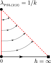
Figure 5: (Color online) (a) Phase diagram for the SU(2) principal chiral model with the coupling constant $\lambda^{\ }_{\mathrm{SU(2)}}$ that is (i) augmented by the WZNW term at level $k=1$ and (ii) perturbed by a symmetry-breaking potential with coupling $h^{\ }$. The critical WZNW theory is at $\lambda^{\ }_{\mathrm{SU(2)}}=1/k$ and is represented on the upper-left corner of the phase diagram by a filled circle. The flow along the upper boundary of the phase diagram is that of the marginally irrelevant current-current perturbation. The lower-left corner of the phase diagram is the Gaussian fixed point of the SU(2) principal chiral model augmented by a WZNW term at level $k=1$, it is depicted by a filled hexagon. The lower-right corner of the phase diagram is the Gaussian fixed point of the O(3) NL$\sigma$M with $\theta$ term at $\theta=\pi$, it is depicted by a filled square. (b) Same as in panel (a) except for the replacement of SU(2) by PSL(2$|$2) and of SU(2)${/}$U(1) by $\mathbb{C}P^{2|1}$ under the assumption that there is no more relevant perturbations than the exactly marginal current-current perturbation at the upper-left corner of the phase diagram. The left vertical boundary Bershadsky99 ; Berkovits99 and the diagonal boundary Guruswamy00 are now lines of critical points (colored in red). The diagonal boundary that connects the upper-left to the lower-right corner is a line of critical points that is argued to have a dual representation in terms of a Thirring model on the one hand or a NL$\sigma$M with a $\theta$ term at $\theta=\pi$ on the other hand.

We are now going to argue that, under certain natural assumptions detailed below, the vertical dashed line of nearly-critical points in region CII of Fig. 4 is described by a NL$\sigma$M with a $\theta$ term at $\theta=\pi$ on the $\mathbb{C}P^{2|1}$ target space [Eq. (72)].

To understand what could prevent the identification of the vertical dashed line of nearly-critical points as realizing the $\mathbb{C}P^{2|1}$ NL$\sigma$M with $\theta$ term at $\theta=\pi$, we are first going to review the connection between the O(3) NL$\sigma$M with the $\theta$ term at $\theta=\pi$ and the $\mathrm{SU(2)}^{\ }_{1}$ WZNW field theory perturbed by the current-current interaction. Affleck87

The O(3) NL$\sigma$M with $\theta$-term at $\theta=\pi$ captures the low-energy and long-wave-length excitations of antiferromagnetic spin-1/2 Heisenberg spin chains. This field theory is related to the $\mathrm{SU(2)}^{\ }_{1}$ WZNW field theory by perturbing the latter with a symmetry-breaking potential (coupling constant $h$), which has the effect of changing the target manifold of the principal chiral model, at $h=0$, to that of the NL$\sigma$M, at $h=\infty$. (See Fig. 5.) When the WZNW model is near its weakly-coupled ultra-violet (UV) Gaussian fixed point, the flow of the coupling $h$ away from this Gaussian fixed point is the strongest and brings the theory into the vicinity of the weakly coupled (UV, Gaussian) fixed point of the O(3) NL$\sigma$M augmented by a $\theta$ term at $\theta=\pi$. In the vicinity of the $\mathrm{SU(2)}^{\ }_{1}$ WZNW critical point, the symmetry-breaking potential (coupling $h$) reduces to the marginally irrelevant current-current interaction up to more irrelevant interactions (some discrete symmetries must here be invoked). When the coupling constant $\lambda$ of the SU(2) principal chiral model augmented by the level $k=1$ WZNW term is close to its critical value $\lambda=1/k=1$, the symmetry-breaking potential generates RG flows that are close to those of O(3) NL$\sigma$M with a $\theta$ term at $\theta=\pi$. When the coupling constant of the SU(2) principal chiral model augmented by the level $k=1$ WZNW term is small, the symmetry-breaking potential generates RG flows that drive the theory very close to the weakly coupled (Gaussian) fixed point of the O(3) NL$\sigma$M with a $\theta$ term at $\theta=\pi$. The envelope of all these RG flows can be thought of as the RG flow from the Gaussian fixed point of the O(3) NL$\sigma$M with a $\theta$ term at $\theta=\pi$ to the $\mathrm{SU(2)}^{\ }_{1}$ WZNW critical point.

The same argument can also be used to relate the principal chiral models defined on the groups $\mathrm{SU}(N)$ and $\mathrm{SO}(M+N)$, augmented by a $k=1$ WZNW term, to the NL$\sigma$M with the target manifold $\mathrm{SU}(N)/\mathrm{SO}(N)$ and $\mathrm{SO}(M+N)/\mathrm{SO}(M)\times\mathrm{SO}(N)$, respectively, when augmented by a $\theta$ term at $\theta=\pi$. This argument is confirmed by exact results obtained from Bethe-Ansatz integrability for these NL$\sigma$Ms. Zamolodchikov92 ; Fendley01

(a) (b)

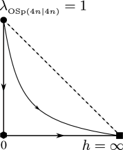
Figure 6: (a) Phase diagram for the SU(2) principal chiral model with the coupling constant $\lambda^{\ }_{\mathrm{SU(2)}}$ that is (i) augmented by the WZNW term at level $k>1$ and (ii) perturbed by a symmetry-breaking potential with coupling $h^{\ }$. The critical WZNW theory is at $\lambda^{\ }_{\mathrm{SU(2)}}=1/k$ and is represented in the phase diagram by a filled circle. The Gaussian fixed point of the SU(2) principal chiral model augmented by a WZNW term at level $k>1$ is depicted by a filled hexagon. The Gaussian fixed point of the O(3) NL$\sigma$M with $\theta$ term at $\theta=\pi$ is depicted by a filled square. The fact that there are operators more relevant than the current-current interaction induced by the symmetry-breaking potential is indicated by the presence of a third axis in coupling space. This third axis quantifies the running of the current-current coupling constant $g^{\ }_{\mathrm{cc}}$ that is marginally irrelevant. The critical point of the O(3) NL$\sigma$M augmented by a $\theta$ term at $\theta=\pi$ is depicted by an open circle. (b) Counterpart to Fig. 5(b) for the case of the WZNW model on $\mathrm{OSp}(4n|4n)$ at level $k=1$ perturbed by a symmetry-breaking potential that projects this WZNW model to the NL$\sigma$M model in the symmetry class AII.

On the other hand, when the level is larger than one (for example, $k>1$ arises from a fine-tuned half-integer spin chain with spin larger than 1/2), the symmetry-breaking potential permits (on symmetry grounds) the appearance of terms more relevant than the current-current interactions in the vicinity of the $\mathrm{SU(2)}^{\ }_{k>1}$ WZNW fixed point. Affleck87 Correspondingly, the flow of the O(3) NL$\sigma$M with a $\theta$ term at $\theta=\pi$ will not reach the $\mathrm{SU(2)}^{\ }_{k>1}$ WZNW critical point, but reaches a different, intermediate fixed point describing the critical behavior of the O(3) NL$\sigma$M with the $\theta$ term at $\theta=\pi$ [see Fig. 6(a)]. This also happens in the $\mathrm{OSp}(2|2)/\mathrm{GL}(1|1)$ NL$\sigma$M with theta term at $\theta=\pi$ describing the critical behavior of the spin-quantum-Hall transition. Gruzberg99 ; Ludwig00

After these preliminary comments, we proceed to the case of interest with $\mathrm{PSL}(2|2)$ symmetry. If we assume that no relevant or marginal interactions other than the marginal current-current interaction are allowed at the $\mathrm{PSL(2|2)}$ WZNW critical point at level $k=1$ when the $\mathrm{PSL}(2|2)\times\mathrm{PSL}(2|2)$ symmetry of the WZNW model is lowered to its diagonal $\mathrm{PSL}(2|2)$ symmetry upon introduction of the symmetry breaking potential (a natural assumption for the level $k=1$ case under consideration), then we obtain with Fig. 5(b) the desired relation between the $\mathrm{PSL(2|2)}$ WZNW theory perturbed by the current-current interaction and the $\mathbb{C}P^{2|1}$ principal chiral model with $\theta$ term at $\theta=\pi$. appendix_potential By analogy with the $\mathrm{SU(2)}^{\ }_{k>1}$ WZNW critical point, we do not expect this assumption to be fulfilled when the level $|k|>1$.

A similar projection from the WZNW model onto the NL$\sigma$M with theta term at $\theta=\pi$ can also be implemented for symmetry class AII, in complete analogy with the case of the projection discussed above from the WZNW model to the NL$\sigma$M in symmetry class CII. For the case of symmetry class AII, consider the WZNW model on $\mathrm{OSp}(4n|4n)$ at level $k=1$. In this case, the coupling constant of the principal chiral model flows away from the WZNW fixed point down towards the weakly coupled WZNW model [see Fig. 6(b)]. Now, we project again to the NL$\sigma$M model in the symmetry class AII with the help of the corresponding symmetry-breaking potential (with coupling constant $h$). When this is done for the weakly coupled WZNW model, this yields the weakly coupled NL$\sigma$M in class AII, the Wess-Zumino term turning into a theta term at $\theta=\pi$ on the AII target space [see Fig. 6(b)]. On the other hand, the most relevant operator in the vicinity of the fixed point of the WZNW model on $\mathrm{OSp}(4n|4n)$ at level $k=1$ which has the symmetries of the symmetry breaking potential is the current-current interaction between the Noether currents. This operator is marginally relevant. Thus, the RG flow emerging from the unstable fixed point of the WZNW model on $\mathrm{OSp}(4n|4n)$ at level $k=1$ ends up in the infrared at the weakly coupled NL$\sigma$M in symmetry class AII [see Fig. 6(b)]. This is one way of understanding that the NL$\sigma$M in class AII with the $\mathbb{Z}^{\ }_{2}$ term always flows to weak coupling (as discussed in Refs. Bardarson07, ; Nomura07, ), for it simply inherits this feature from the RG flow of the underlying WZNW model.

In summary, based on this reasoning we argue that the line of nearly-critical points in region CII of Fig. 4 (the vertical dashed line in region CII of Fig. 4) has two descriptions; one in terms of the $\mathrm{PSL}(2|2)$ WZNW model perturbed by current-current interactions, and one in terms of the $\mathbb{C}P^{2|1}$ NL$\sigma$M at $\theta=\pi$ ($\mathbb{Z}^{\ }_{2}$ topological term). These descriptions are dual to each other in the sense that, in the vicinity of the origin of our global phase diagram in Fig. 4 the $\mathrm{PSL}(2|2)$ WZNW model is weakly perturbed, whereas the $\mathbb{C}P^{2|1}$ NL$\sigma$M is strongly interacting. On the other hand, for large values of the coupling constant $g^{\ }_{\mathrm{M}^{\prime}}$ of the current-current interaction about the Dirac point, a measure of the distance downwards along the dotted line away from the clean Dirac point at the center of Fig. 4, the resulting Thirring model is strongly interacting whereas the $\mathbb{C}P^{2|1}$ NL$\sigma$M is weakly interacting. We recall that, because the coupling constant $g^{\ }_{\mathrm{M}^{\prime}}$ is exactly marginal, and so is the coupling constant of the corresponding NL$\sigma$M,Gade91-93 it is possible to continuously interpolate between these two limits by tuning $g^{\ }_{\mathrm{M}^{\prime}}$. (The possibility of such a duality was also discussed, independently and from a different perspective, in Ref. Mitev08, , Candu09, , and Candu10, .)

V Discussion

V.1 $\mathbb{Z}^{\ }_{2}$ topological term in the symmetry class CII of two-dimensional Anderson localization

A systematic study of random Dirac fermions in $d$-dimensional space provides a road-map to uncovering universal properties of Anderson localization. This is so because random Dirac fermions build a bridge between models for Anderson localization that are defined on lattices – and thus are non-universal – and effective field theories (NL$\sigma$Ms) that solely depend on the underlying symmetries and dimensionality of space – and as such are universal.

In one-dimensional space, Dirac fermions generically emerge after linearization of the energy dispersion around the Fermi energy in the clean limit. The effects of weak static disorder are then elegantly encoded by a description of quasi-one-dimensional quantum transport in terms of diffusive processes on non-compact symmetric spaces.Huffmann90 ; Brouwer00 ; Mudry00 ; Titov01 ; Brouwer03 ; Brouwer05 This long-wave length description is sufficiently fine to account for non-perturbative effects such as parity effects in the numbers of propagating channels in the chiral symmetry classes AIII, CII, and BDI. Brouwer98 A parity effect can also be derived for the symplectic symmetry class AII in quasi-one dimension. Zirnbauer92 ; Takane04 Although the latter parity effect is not generic in quasi-one-dimensional space because of the fermion-doubling obstruction, it is generic on one-dimensional boundaries of two-dimensional $\mathbb{Z}^{\ }_{2}$-topological band insulators.Obuse07

Dirac fermions are the exception rather than the rule in band theory when the dimensionality of space $d$ is larger than one. Fine-tuning between the lattice and the hopping amplitudes is needed to select a linear energy dispersion. There is a parallel to this fact in the context of Anderson localization.

For example, in two-dimensional space, the symmetries respected by the static disorder do not enforce, on their own, the presence of WZNW or $\mathbb{Z}^{\ }_{2}$-topological terms in the NL$\sigma$M effective long-wave length description of the physics of localization.

Ludwig et al.Ludwig94 (Nersesyan et al.Nersesyan95 ) have shown that non-perturbative effects can modify the localization properties encoded by the two-dimensional NL$\sigma$M with a WZNW term in symmetry class AIII when studying the random Dirac Hamiltonian with $\mathrm{N}^{\ }_{\mathrm{f}}=1$ ($\mathrm{N}^{\ }_{\mathrm{f}}>1$) flavors. Analogous physics can appear in symmetry classes DIII and CI in two spatial dimensions. Schnyder08 ; Schnyder09b ; Schnyder09a However, because of the fermion-doubling obstruction, these conditions cannot be met in purely two-dimensional lattice models for Anderson localization.

On the other hand, they can always be fulfilled on the two-dimensional boundaries of three-dimensional topological band insulators (that are characterized by an integer topological index). Schnyder08 ; Ryu10b

A similar situation holds for the $\mathbb{Z}^{\ }_{2}$-topological terms. The number of Dirac flavors $\mathrm{N}^{\ }_{\mathrm{f}}$ matters crucially to obtain a $\mathbb{Z}^{\ }_{2}$-topological term in symmetry class AII as shown by Ryu et al. in Ref. Ryu07b, . In the present paper, we have completed the derivation of topological terms of two-dimensional NL$\sigma$M by constructing the $\mathbb{Z}^{\ }_{2}$-topological term for a NL$\sigma$M in symmetry class CII as a sign ambiguity in the Pfaffian of disordered Majorana spinors. Our derivation suggests that this $\mathbb{Z}^{\ }_{2}$-topological term cannot arise from two-dimensional local lattice models of Anderson localization because of the fermion-doubling obstruction, but requires a three-dimensional topological band insulator with two-dimensional boundaries.

V.2 Global phase diagram at the band center

The main results of this paper are summarized in Fig. 4. They apply to $\mathrm{N}^{\ }_{\mathrm{f}}=2$ flavors of random Dirac fermions.

Figure 4 should be compared with Fig. 9 from Ref. Ludwig94, that captures the phase diagram for $\mathrm{N}^{\ }_{\mathrm{f}}=1$ flavors of random Dirac fermions or, more precisely, with its projection onto the plane $g^{\ }_{\mathrm{A}}=0$ in Ref. Ludwig94, ($\Delta^{\ }_{\mathrm{A}}=0$ in the notation of Ref. Ludwig94, ). The phase diagram in Fig. 4 is also obtained after projecting a three-dimensional flow to a two-dimensional subspace of in coupling constant space.

The three chiral phases AIII, BDI, and CII in Fig. 4 meet at the origin of the phase diagram. This meeting point realizes the clean Dirac limit. We showed that analytical continuation of the disorder at the level of the Dirac fermions allows one to move between the BDI and CII phases. However, at the microscopic scale of the two-dimensional lattice model that realizes the BDI phase, this analytical continuation is meaningless. This is yet another manifestation of the fermion-doubling obstruction. A realization as a local lattice model of the CII phase in Fig. 4 must go through the two-dimensional boundary of a three-dimensional topological band insulator.

The quadrant BDI in Fig. 4 is fairly well understood if we assume that the perturbative flows to the nearly-critical dashed line extend all the way to the boundary D. Bulk Mudry03 and boundary Obuse08 multifractality and an analytic dependence of the conductance on the disorder strength $g^{\ }_{\mathrm{M}}$ at the band center $E=0$ Ryu07a are governed in the thermodynamic limit by their dependence on $g^{\ }_{\mathrm{M}}$ along the nearly-critical dashed line.

The dashed line in region CII of Fig. 4 is a line of nearly-critical points, each of which is captured by a projected Thirring model. We have argued that the strong coupling regime of this theory is “dual” to a weakly-coupled NL$\sigma$M augmented by a $\mathbb{Z}^{\ }_{2}$ topological term with the target space of symmetry class CII.

We would like to emphasize that the RG flows in the CII quadrant of Fig. 4, first away from and then to the nearly-critical plane defined by the dashed line and the out-of-plane $g^{\ }_{a^{\prime}}$ axis, are perturbative in $g^{\prime}_{\pm}$ (nonperturbative in $g^{\ }_{a^{\prime}}$). They are derived under the assumption that no relevant or marginal interactions other than the current-current interactions are allowed. The continuation of these flows to strong coupling is a conjecture. At strong coupling, it is tempting to ask if these two-parameter flows might be captured by a NL$\sigma$M. Evidently, a NL$\sigma$M whose target space is a symmetric target space will not do since it would only be characterized by one running coupling constant. A NL$\sigma$M on a homogeneous but not symmetric target space with two independent coupling constants in addition to the Gade term would do. (We refer the reader to Ref. Friedan85, for a systematic study of NL$\sigma$M on Riemannnian manifolds, of which homogeneous and symmetric spaces are special examples, as is explained in the context of disordered systems in Ref. footnote: homogeneous space, .) We propose that this scenario is captured by a NL$\sigma$M with the following homogeneous, but not symmetric target space ($n$ is an integer, see Appendix E)

$$\mathrm{GL}(2n|2n)/[\mathrm{OSp}(n|n)\times\mathrm{OSp}(n|n)].$$ (75)

The situation here is analogous to the NL$\sigma$M discussed in Ref. footnote: homogeneous space, in the context of the random-bond Ising model in two dimensions. The NL$\sigma$M on the homogeneous target space in Eq. (75) has two coupling constants [in addition to the coupling constant of the “Gade” term (“projected out” in our global phase diagram in Fig. 4), of the kind that we previously denoted by $g^{\ }_{a^{\prime}}$ in the present paper]. The NL$\sigma$M on this homogeneous space interpolates between the two NL$\sigma$Ms on the symmetric target spaces corresponding to symmetry classes CII and AII, which are specific limits within the 2-parameter coupling constant space of the NL$\sigma$M on this homogeneous space (in a manner analogous to the situation discussed in Ref. footnote: homogeneous space, ). See Appendix E for more details.

(a) (b)

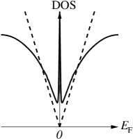
Figure 7: (a) Global density of states (DOS) of a two-dimensional disorder-free tight-binding model with sublattice symmetry and an even number equal to or larger than 2 of non-equivalent discrete Fermi points at the band center. The dashed line is the global DOS of the corresponding disorder-free Dirac fermions in two dimensions. (b) Effect of weak disorder for symmetry class AII without the $\mathbb{Z}^{\ }_{2}$ topological term (the surface states of a three-dimensional time-reversal-symmetric weak topological insulator), the symmetry class relevant to the quadrant CII when perturbed by a finite chemical potential. The band center is a critical energy at which, according to Eq. (77), the global DOS diverges. This critical energy separates two metallic phases.

V.3 Weak breaking of the chiral symmetry in the vicinity of the band center

The effects of a finite Fermi energy $E^{\ }_{\mathrm{F}}$ on the physics of localization for the quadrants BDI and CII in Fig. 4 are dramatic in that, in both cases, a finite $E^{\ }_{\mathrm{F}}$ breaks the chiral symmetry chS.

Turning on a finite Fermi energy $E^{\ }_{\mathrm{F}}$ in the quadrant BDI in Fig. 4 reduces the symmetry class to AI. All states at finite $E^{\ }_{\mathrm{F}}$ are then localized. Evers08 The band center is a quantum critical point separating two insulating phases, one defined by $E^{\ }_{\mathrm{F}}<0$ and another one defined by $E^{\ }_{\mathrm{F}}>0$, very much as is the case in the integer quantum Hall effect (IQHE) (see Ref. Evers08, for a review on plateau transitions in the IQHE). The global density of states $\nu(E^{\ }_{\mathrm{F}})$ diverges as

$$\nu(E^{\ }_{\mathrm{F}})\sim\frac{1}{|E^{\ }_{\mathrm{F}}|}\exp\left(-c|\ln|E^{\ }_{\mathrm{F}}||^{2/3}\right)$$ (76)

with $c$ a non-universal number when $E^{\ }_{\mathrm{F}}$ approaches the band center. Mudry03

Turning on a finite Fermi energy $E^{\ }_{\mathrm{F}}$ in the quadrant CII in Fig. 4 reduces the symmetry class to AII but without the $\mathbb{Z}^{\ }_{2}$ topological term. Indeed, the random Dirac Hamiltonian at a finite chemical potential has now two flavors that are coupled by the disorder. This corresponds to two Dirac cones in any underlying microscopic model that are generically coupled by the disorder. The global density of states $\nu(E^{\ }_{\mathrm{F}})$ is again diverging according to the law

$$\nu(E^{\ }_{\mathrm{F}})\sim\frac{1}{|E^{\ }_{\mathrm{F}}|}\exp\left(-c^{\prime}|\ln|E^{\ }_{\mathrm{F}}||^{2/3}\right)$$ (77)

with $c^{\prime}$ a non-universal number when $E^{\ }_{\mathrm{F}}$ approaches the band center. Mudry03 The state at the band center is critical. (The robustness to strong disorder of the critical behavior of the band center in the chiral classes is well documented in quasi-one and two dimensions. Motrunich02 ) However, contrary to the quadrant BDI in Fig 4, the band center is not any more a quantum critical point separating two insulating phases. Indeed, the localized nature as a function of the chemical potential of these two-dimensional states is that of the surface states of a three-dimensional time-reversal-symmetric weak topological insulator. The issue of Anderson localization as a function of the chemical potential for such surface states was recently discussed in Refs. Ringel11, and Mong11, . According to the numerical study in Ref. Mong11, (corresponding to the case of a mean value $\bar{m}=0$ of the random mass $m$ in Ref. Mong11, ), these surface states remain extended (metallic) in the presence of disorder even though the characteristic energy at which the upturn of the diverging global DOS becomes sizable relative to the clean DOS shown in Fig. 7(a) is exponentially small for weak disorder. Mudry03

Appendix A The sign ambiguity of a Pfaffian

In this section, we are going to argue that the dashed line in the phase diagram of Fig. 4 that belongs to the chiral symplectic class CII has the particularity that, within the fermionic replica NL$\sigma$M representation, there appears a $\mathbb{Z}^{\ }_{2}$-topological term in addition to the standard kinetic energy.

To this end, it will be useful to enlarge the dimensionality of the representation of the Dirac Hamiltonian by a factor of 2 in order to treat the isospin-1/2 TRS. To avoid ambiguities, we will use the Greek letters for the Pauli matrices acting on the three relevant two-dimensional subspaces – $\rho$ in flavor subspace, $\sigma$ in Lorentz subspace, and $\tau$ in the time-reversal subspace to be introduced below – as subindices to specify the chosen representations. In this section we use indices $x,y,z$, instead of $1,2,3$, in the $\sigma$ and $\tau$ subspaces. For example, we shall denote the Dirac Hamiltonian (12) when Eq. (14) holds by

$$\begin{split}&\mathcal{H}^{\ }_{\rho,\sigma}:=\begin{pmatrix}0&D^{\ }_{\sigma}\\ D^{{\dagger}}_{\sigma}&0\end{pmatrix}^{\ }_{\rho},\\ &D^{\ }_{\sigma}:=\sigma^{\ }_{x}\left(-{i}\partial^{\ }_{x}+A^{\ }_{x}\right)+\sigma^{\ }_{y}\left(-{i}\partial^{\ }_{y}+A^{\ }_{y}\right)\\ &\hphantom{D^{\ }_{\sigma}:=}+\sigma^{\ }_{z}\,M^{\ }_{z}+\sigma^{\ }_{0}\,M^{\ }_{0},\end{split}$$ (78a)

where $$A^{\ }_{\mu}=-{i}a^{\prime}_{\mu}\in{i}\mathbb{R} M^{\ }_{z}=-{i}m^{\prime}_{z}\in{i}\mathbb{R} M^{\ }_{0}=m^{\prime}_{0}\in\mathbb{R}$$, , , and with the simultaneous chS

$$(\rho^{\ }_{z}\otimes\sigma^{\ }_{0})\mathcal{H}^{\ }_{\rho,\sigma}(\rho^{\ }_{z}\otimes\sigma^{\ }_{0})=-\mathcal{H}^{\ }_{\rho,\sigma}$$ (78b)

and isospin-1/2 TRS

$$({i}\rho^{\ }_{0}\otimes\sigma^{\ }_{y})\mathcal{H}^{T}_{\rho,\sigma}(-{i}\rho^{\ }_{0}\otimes\sigma^{\ }_{y})=\mathcal{H}^{\ }_{\rho,\sigma}.$$ (78c)

A.1 Fermionic functional integral representation of the retarded Green’s function

The generating function for the retarded Green’s function is the partition function

$$\begin{split}Z:=&\,\int\mathcal{D}\left[\bar{\chi},\chi\right]\exp\left(-\int\mathrm{d}^{2}\,r\,\mathcal{L}\right),\\ \mathcal{L}:=&-{i}\bar{\chi}({i}\eta-\mathcal{H})^{\ }_{\rho,\sigma}\chi.\end{split}$$ (79a)

Here, we have chosen

$$\bar{\chi}\equiv\begin{pmatrix}\bar{\chi}^{\ }_{1}&\bar{\chi}^{\ }_{2}\end{pmatrix}^{\ }_{\rho}\equiv\begin{pmatrix}\bar{\chi}^{\ }_{1\uparrow}&\bar{\chi}^{\ }_{1\downarrow}&\bar{\chi}^{\ }_{2\uparrow}&\bar{\chi}^{\ }_{2\downarrow}\end{pmatrix}^{\ }_{\rho,\sigma}$$ (79b)

to be a 4-component row spinor with Grassmann-valued entries. Similarly,

$$\chi\equiv\begin{pmatrix}\chi^{\ }_{1}\\ \chi^{\ }_{2}\end{pmatrix}^{\ }_{\rho}\equiv\begin{pmatrix}\chi^{\ }_{1\uparrow}\\ \chi^{\ }_{1\downarrow}\\ \chi^{\ }_{2\uparrow}\\ \chi^{\ }_{2\downarrow}\end{pmatrix}^{\ }_{\rho,\sigma}$$ (79c)

is a 4-component column spinor with Grassmann-valued entries. All 8 Grassmann-valued entries labeled by the flavor indices $1$ and $2$ on which the matrices $(\rho^{\ }_{0},\rho^{\ }_{x},\rho^{\ }_{y},\rho^{\ }_{z})$ act and by the Lorentz indices $\uparrow$ and $\downarrow$ on which the matrices $(\sigma^{\ }_{0},\sigma^{\ }_{x},\sigma^{\ }_{y},\sigma^{\ }_{z})$ act are independent. For the retarded Green’s function, $\eta>0$.

It is useful to make the TRS (78c) explicit. To this end, following Ref. Efetov80, , we make the manipulation

$$\begin{split}\mathcal{L}=&\,-{i}\,\bar{\chi}({i}\eta-\mathcal{H})^{\ }_{\rho,\sigma}\chi\\ =&\,+{i}\,\chi^{T}({i}\eta-\mathcal{H})^{T}_{\rho,\sigma}\bar{\chi}^{T}\\ =&\,-{i}\,\chi^{T}(-{i}\rho^{\ }_{0}\otimes\sigma^{\ }_{y})({i}\eta-\mathcal{H})^{\ }_{\rho,\sigma}(-{i}\rho^{\ }_{0}\otimes\sigma^{\ }_{y}\bar{\chi}^{T})\\ =&\,-{i}\,\bar{\Psi}({i}\eta-\mathcal{H})^{\ }_{\rho,\tau,\sigma}\Psi\end{split}$$ (80a)

by which we have doubled the number of Grassmann-valued entries in $$\bar{\Psi} \Psi$$ and through the definitions

$$\begin{split}({i}\eta-\mathcal{H})^{\ }_{\rho,\tau,\sigma}:=&\,({i}\eta-\mathcal{H})^{\ }_{\rho,\sigma}\otimes\tau^{\ }_{0},\end{split}$$ (80b)

and

$$\begin{split}\bar{\Psi}:=&\,\frac{1}{\sqrt{2}}\left(\begin{array}[]{cccc}\bar{\chi}^{\ }_{\uparrow}&\bar{\chi}^{\ }_{\downarrow}&\chi^{T}_{\downarrow}&-\chi^{T}_{\uparrow}\end{array}\right)^{\ }_{\tau,\sigma},\\ \Psi:=&\,\frac{1}{\sqrt{2}}\left(\begin{array}[]{c}\chi^{\ }_{\uparrow}\\ \chi^{\ }_{\downarrow}\\ -\bar{\chi}^{T}_{\downarrow}\\ \bar{\chi}^{T}_{\uparrow}\end{array}\right)^{\ }_{\tau,\sigma}.\end{split}$$ (80c)

Here, the subindex $\tau$ denotes the, by now, explicit time-reversal subspace that is spanned by the unit $2\times 2$ matrix $\tau^{\ }_{0}$ and the three Pauli matrices $(\tau^{\ }_{1},\tau^{\ }_{2},\tau^{\ }_{3})$. Of course, the number of independent Grassmann-valued entries remains unchanged in the representation (80c) as the TRS (78c) is now represented by the constraint

$$\bar{\Psi}=\Psi^{T}(-{i}\rho^{\ }_{0}\otimes\tau^{\ }_{x}\otimes\sigma^{\ }_{y}).$$ (81)

On the other hand, the representation of the chS (78b) is

$$\rho^{\ }_{z}\otimes\tau^{\ }_{0}\otimes\sigma^{\ }_{0}\mathcal{H}^{\ }_{\rho,\tau,\sigma}\rho^{\ }_{z}\otimes\tau^{\ }_{0}\otimes\sigma^{\ }_{0}=-\mathcal{H}^{\ }_{\rho,\tau,\sigma}.$$ (82)

Instead of Eq. (81), we seek a representation of the TRS in terms of 8-component Grassmann-valued spinors obeying the Majorana constraint

$$\bar{\psi}=\psi^{T}(-{i}\rho^{\ }_{0}\otimes\tau^{\ }_{0}\otimes\sigma^{\ }_{y}).$$ (83)

This can be achieved by observing that the “square root” of $\tau^{\ }_{x}$ is given by

$$\tau^{\ }_{x}=-{i}\,\tau^{T}_{z-y}\tau^{\ }_{z-y},\qquad\tau^{\ }_{z-y}:=\frac{\tau^{\ }_{z}-\tau^{\ }_{y}}{\sqrt{2}}.$$ (84)

Now, we take advantage of the fact that the kernel (80b) commutes with

$$T^{\ }_{z-y}:=\rho^{\ }_{0}\otimes\tau^{\ }_{z-y}\otimes\sigma^{\ }_{0}$$ (85)

so that

$$\begin{split}\mathcal{L}=&\,-{i}\bar{\Psi}({i}\eta-\mathcal{H})^{\ }_{\rho,\tau,\sigma}\Psi\\ =&\,{\Psi}^{T}T^{T}_{z-y}({i}\rho^{\ }_{0}\otimes\tau^{\ }_{0}\otimes\sigma^{\ }_{y})({i}\eta-\mathcal{H})^{\ }_{\rho,\tau,\sigma}T^{\ }_{z-y}\Psi\\ \equiv&\,-\bar{\psi}({i}\eta-\mathcal{H})^{\ }_{\rho,\tau,\sigma}\psi\end{split}$$ (86a)

where

$$\psi:=T^{\ }_{z-y}\Psi$$ (86b)

determines $\bar{\psi}$ through the Majorana constraint Eq. (83) that follows because of the isospin-1/2 TRS. In view of the Majorana constraint (83), the isospin-1/2 TRS is now equivalent to the global $\mathrm{O}(2)$ invariance under the transformation

$$\bar{\psi}\to\bar{\psi}\,(\rho^{\ }_{0}\otimes\sigma^{\ }_{0}\otimes O^{T}_{\tau}),\qquad\psi\to(\rho^{\ }_{0}\otimes\sigma^{\ }_{0}\otimes O^{\ }_{\tau})\,\psi$$ (87)

for any $2\times 2$ orthogonal matrix $O^{\ }_{\tau}$ acting in the $\tau$ subspace.

Finally, it is time to make use of the chS (78b). By making the flavor subspace explicit,

$$\begin{split}\mathcal{L}=&\bar{\psi}^{\ }_{1}D^{\ }_{\tau,\sigma}\psi^{\ }_{2}+\bar{\psi}^{\ }_{2}D^{{\dagger}}_{\tau,\sigma}\psi^{\ }_{1}\\ &\,-{i}\eta\left(\bar{\psi}^{\ }_{1}\psi^{\ }_{1}+\bar{\psi}^{\ }_{2}\psi^{\ }_{2}\right),\end{split}$$ (88a)

where ($$a^{\prime}_{\mu},m^{\prime}_{z},m^{\prime}_{0}\in\mathbb{R}$$)

$$\begin{split}&D^{\ }_{\tau,\sigma}:=\tau^{\ }_{0}\otimes\left(-{i}\sigma^{\ }_{\mu}\partial^{\ }_{\mu}+V\right),\\ &V:={i}\sigma^{\ }_{\mu}a^{\prime}_{\mu}-{i}\sigma^{\ }_{z}m^{\prime}_{z}+\sigma^{\ }_{0}m^{\prime}_{0},\end{split}$$ (88b)

acts on the two independent 4-component Grassmann-valued spinors $$\psi^{\ }_{1} \psi^{\ }_{2} \bar{\psi}^{\ }_{1} \bar{\psi}^{\ }_{2} \Sigma^{\ }_{y}:=\tau^{\ }_{0}\otimes\sigma^{\ }_{y}$$ and while the spinors and obey the Majorana condition ()

$$\bar{\psi}^{\ }_{1}=\psi^{T}_{1}(-{i}\Sigma^{\ }_{y}),\qquad\bar{\psi}^{\ }_{2}=\psi^{T}_{2}(-{i}\Sigma^{\ }_{y}).$$ (88c)

With the help of the identity

$$\bar{\psi}^{\ }_{2}D^{{\dagger}}_{\tau,\sigma}\psi^{\ }_{1}=-\psi^{T}_{1}D^{*}_{\tau,\sigma}\bar{\psi}^{T}_{2}=\bar{\psi}^{\ }_{1}D^{\ }_{\tau,\sigma}\psi^{\ }_{2},$$ (89)

we arrive at

$$\mathcal{L}=2\,\bar{\psi}^{\ }_{1}D^{\ }_{\tau,\sigma}\psi^{\ }_{2}-{i}\eta\left(\bar{\psi}^{\ }_{1}\psi^{\ }_{1}+\bar{\psi}^{\ }_{2}\psi^{\ }_{2}\right).$$ (90)

This presentation of the Lagrangian reveals that, upon quantization, $\bar{\psi}^{\ }_{1}$ and $\psi^{\ }_{2}$ form a canonical pair of fermionic operators. In other words, because of the chS, the kinetic part $\bar{\psi}^{\ }_{1}D^{\ }_{\tau,\sigma}\psi^{\ }_{2}$ of the Lagrangian is invariant under any global $\mathrm{U}(2)$ transformation

$$\bar{\psi}^{\ }_{1}\to\bar{\psi}^{\ }_{1}(\sigma^{\ }_{0}\otimes U^{{\dagger}}_{\tau}),\qquad\psi^{\ }_{2}\to(\sigma^{\ }_{0}\otimes U^{\ }_{\tau})\,\psi^{\ }_{2},$$ (91)

where $U^{\ }_{\tau}$ is a $2\times 2$ unitary matrix acting in the $\tau$ subspace.

A.2 Replicas and disorder averaging

We now assume that $a^{\prime}_{x}$, $a^{\prime}_{y}$, $m^{\prime}_{z}$, and $m^{\prime}_{0}$ from Eq. (88) are all white-noise distributed with the same variance $g$. In doing so, we limit ourselves to the nearly-critical line of region CII in Fig. 4.

We replicate the Lagrangian $\mathsf{N}^{\ }_{\mathrm{r}}$ times,

$$\begin{split}\mathcal{L}^{\ }_{\mathsf{N}^{\ }_{\mathrm{r}}}=&\,\sum_{\mathsf{a}=1}^{2\mathsf{N}^{\ }_{\mathrm{r}}}\big{[}2\bar{\psi}^{\ }_{\mathsf{a}1}(-i\sigma_{\mu}\partial_{\mu}+V)\psi^{\ }_{\mathsf{a}2}\\ &\,-{i}\eta\left(\bar{\psi}^{\ }_{\mathsf{a}1}\psi^{\ }_{\mathsf{a}1}+\bar{\psi}^{\ }_{\mathsf{a}2}\psi^{\ }_{\mathsf{a}2}\right)\big{]}.\end{split}$$ (92)

This Lagrangian is invariant under any global $\mathrm{O}(2\mathsf{N}^{\ }_{\mathrm{r}})$ rotation in the $\tau$ and replica subspaces. After disorder averaging has been performed, we arrive at the interacting Lagrangian

$$\begin{split}\mathcal{L}^{\ }_{\mathsf{N}^{\ }_{\mathrm{r}}}=&\,2\sum_{\mathsf{a}=1}^{2\mathsf{N}^{\ }_{\mathrm{r}}}\bm{d}^{{\dagger}}_{\mathsf{a}}\left(-{i}\sigma^{\ }_{\mu}\partial^{\ }_{\mu}\right)\bm{d}^{\ }_{\mathsf{a}}\\ &\,+{i}\eta\sum_{\mathsf{a}=1}^{2\mathsf{N}^{\ }_{\mathrm{r}}}\left[\bm{d}^{{\dagger}}_{\mathsf{a}}{i}\sigma^{\ }_{y}(\bm{d}^{{\dagger}}_{\mathsf{a}})^{T}+\bm{d}^{T}_{\mathsf{a}}{i}\sigma^{\ }_{y}\bm{d}^{\ }_{\mathsf{a}}\right]\\ &\,+8g\sum_{\mathsf{a},\mathsf{b}=1}^{2\mathsf{N}^{\ }_{\mathrm{r}}}\left(\vec{S}^{\ }_{\mathsf{a}}\cdot\vec{S}^{\ }_{\mathsf{b}}-\frac{1}{4}n^{\ }_{\mathsf{a}}n^{\ }_{\mathsf{b}}\right).\end{split}$$ (93a)

Here, since $$\bar{\psi}^{\ }_{1} \psi^{\ }_{2} \mathsf{a}=1,\cdots,2\mathsf{N}^{\ }_{\mathrm{r}}$$ and are canonically conjugate, we have introduced the following notation for any ,

$$\begin{split}&\bm{d}^{{\dagger}}_{\mathsf{a}}:=\bar{\psi}^{\ }_{\mathsf{a}1},\qquad\bm{d}^{\ }_{\mathsf{a}}:=\psi^{\ }_{\mathsf{a}2},\\ &\vec{S}^{\ }_{\mathsf{a}}:=\frac{1}{2}\bm{d}^{{\dagger}}_{\mathsf{a}}\vec{\sigma}\bm{d}^{\ }_{\mathsf{a}},\qquad n^{\ }_{\mathsf{a}}:=\bm{d}^{{\dagger}}_{\mathsf{a}}\bm{d}^{\ }_{\mathsf{a}}.\end{split}$$ (93b)

It is worth remembering that the replicated “spin” $\vec{S}^{\ }_{\mathsf{a}}$ in the $t$-$J$-like Lagrangian (93a) originates from the $\sigma$ subspace and not the true electronic spin-1/2. When $\eta=0$ and in accordance with the global symmetry (91), the action is invariant under any global $\mathrm{U}(2\mathsf{N}^{\ }_{\mathrm{r}})$ rotation

$$\bm{d}^{{\dagger}}_{\mathsf{a}}\to\bm{d}^{{\dagger}}_{\mathsf{b}}U^{*}_{\mathsf{a}\mathsf{b}},\qquad\bm{d}^{\ }_{\mathsf{a}}\to U^{\ }_{\mathsf{a}\mathsf{c}}\bm{d}^{\ }_{\mathsf{c}},\qquad U^{*}_{\mathsf{a}\mathsf{b}}U^{\ }_{\mathsf{a}\mathsf{c}}=\delta_{\mathsf{b}\mathsf{c}},$$ (94)

while, in accordance with the global symmetry (87), any non-zero $\eta$ breaks this symmetry down to the global $\mathrm{O}(2\mathsf{N}^{\ }_{\mathrm{r}})$ rotation

$$\bm{d}^{T}_{\mathsf{a}}\to\bm{d}^{T}_{\mathsf{b}}O^{\ }_{\mathsf{a}\mathsf{b}},\qquad\bm{d}^{\ }_{\mathsf{a}}\to O^{\ }_{\mathsf{a}\mathsf{c}}\bm{d}^{\ }_{\mathsf{c}},\qquad O^{\ }_{\mathsf{a}\mathsf{b}}O^{\ }_{\mathsf{a}\mathsf{c}}=\delta_{\mathsf{b}\mathsf{c}},$$ (95)

where summation over repeated indices is assumed.

A.3 Hubbard-Stratonovich transformation

It is time to introduce auxiliary (Hubbard-Stratonovich) fields that decouple the interactions among replicas. A possible channel for decoupling is singlet superconductivity as it is favored by the symmetry breaking term $\eta$. Hence for any $\mathsf{a},\mathsf{b}=1,\cdots,2\mathsf{N}^{\ }_{\mathrm{r}}$, we introduce the order parameters

$$\begin{split}\mathcal{O}^{{\dagger}}_{\mathsf{a}\mathsf{b}}:=&\,\frac{-1}{\sqrt{2}}\bm{d}^{{\dagger}}_{\mathsf{a}}{i}\sigma^{\ }_{y}(\bm{d}^{{\dagger}}_{\mathsf{b}})^{T}\\ =&\,\frac{-1}{\sqrt{2}}\left(d^{{\dagger}}_{\mathsf{a}\uparrow}d^{{\dagger}}_{\mathsf{b}\downarrow}-d^{{\dagger}}_{\mathsf{a}\downarrow}d^{{\dagger}}_{\mathsf{b}\uparrow}\right),\\ \mathcal{O}^{\ }_{\mathsf{a}\mathsf{b}}:=&\,\frac{1}{\sqrt{2}}\bm{d}^{T}_{\mathsf{a}}{i}\sigma^{\ }_{y}\bm{d}^{\ }_{\mathsf{b}}\\ =&\,\frac{1}{\sqrt{2}}\left(d^{\ }_{\mathsf{a}\uparrow}d^{\ }_{\mathsf{b}\downarrow}-d^{\ }_{\mathsf{a}\downarrow}d^{\ }_{\mathsf{b}\uparrow}\right),\end{split}$$ (96)

in terms of which the “exchange term” becomes

$$\vec{S}^{\ }_{\mathsf{a}}\cdot\vec{S}^{\ }_{\mathsf{b}}-\frac{1}{4}n^{\ }_{\mathsf{a}}n^{\ }_{\mathsf{b}}=-\mathcal{O}^{{\dagger}}_{\mathsf{a}\mathsf{b}}\mathcal{O}^{\ }_{\mathsf{a}\mathsf{b}},$$ (97)

and, in turn, the Lagrangian becomes

$$\begin{split}\mathcal{L}^{\ }_{\mathsf{N}^{\ }_{\mathrm{r}}}=&\,2\sum_{\mathsf{a}=1}^{2\mathsf{N}^{\ }_{\mathrm{r}}}\bm{d}^{{\dagger}}_{\mathsf{a}}\left(-{i}\sigma^{\ }_{\mu}\partial^{\ }_{\mu}\right)\bm{d}^{\ }_{\mathsf{a}}\\ &\,+{i}\sqrt{2}\,\eta\sum_{\mathsf{a}=1}^{2\mathsf{N}^{\ }_{\mathrm{r}}}\left(\mathcal{O}^{\ }_{\mathsf{a}\mathsf{a}}-\mathcal{O}^{{\dagger}}_{\mathsf{a}\mathsf{a}}\right)\\ &\,-8g\sum_{\mathsf{a},\mathsf{b}=1}^{2\mathsf{N}^{\ }_{\mathrm{r}}}\mathcal{O}^{{\dagger}}_{\mathsf{a}\mathsf{b}}\mathcal{O}^{\ }_{\mathsf{a}\mathsf{b}}.\end{split}$$ (98)

The interacting term is then decoupled by the $2\mathsf{N}^{\ }_{\mathrm{r}}\times 2\mathsf{N}^{\ }_{\mathrm{r}}$ Hubbard-Stratonovich field $\Delta^{\ }_{\mathsf{a}\mathsf{b}}$ and its complex conjugate $\Delta^{*}_{\mathsf{a}\mathsf{b}}$,

$$\begin{split}\mathcal{L}^{\ }_{\mathsf{N}^{\ }_{\mathrm{r}}}=&\,2\sum_{\mathsf{a}=1}^{2\mathsf{N}^{\ }_{\mathrm{r}}}\bm{d}^{{\dagger}}_{\mathsf{a}}\left(-{i}\sigma^{\ }_{\mu}\partial^{\ }_{\mu}\right)\bm{d}^{\ }_{\mathsf{a}}\\ &\,+{i}\sqrt{2}\,\eta\sum_{\mathsf{a}=1}^{2\mathsf{N}^{\ }_{\mathrm{r}}}\left(\mathcal{O}^{\ }_{\mathsf{a}\mathsf{a}}-\mathcal{O}^{{\dagger}}_{\mathsf{a}\mathsf{a}}\right)\\ &\,+\sum_{\mathsf{a},\mathsf{b}=1}^{2\mathsf{N}^{\ }_{\mathrm{r}}}\left(\frac{1}{8g}\Delta^{*}_{\mathsf{b}\mathsf{a}}\Delta^{\ }_{\mathsf{b}\mathsf{a}}-\mathcal{O}^{{\dagger}}_{\mathsf{a}\mathsf{b}}\Delta^{\ }_{\mathsf{b}\mathsf{a}}-\mathcal{O}^{\ }_{\mathsf{a}\mathsf{b}}\Delta^{*}_{\mathsf{b}\mathsf{a}}\right).\end{split}$$ (99)

No approximation has yet been invoked. As the interacting Lagrangian (99) is not readily tractable, we shall restrict the path integral to slowly varying bosonic degrees of freedom (Nambu-Goldstone bosons). We first look for a diffusive saddle point of the Lagrangian (99). In the diffusive regime, the auxiliary field $\Delta^{\ }_{\mathsf{a}\mathsf{b}}$ (spontaneously) breaks the global $\mathrm{U}(2\mathsf{N}^{\ }_{\mathrm{r}})$ symmetry, along the symmetry breaking “direction” controlled by the symmetry breaking term $\eta$. Thus, the spatially homogeneous configuration

$$\Delta^{\ }_{0\mathsf{a}\mathsf{b}}=-{i}\left|\Delta^{\ }_{0}\right|\delta^{\ }_{\mathsf{a}\mathsf{b}}$$ (100)

should be a representative diffusive saddle point, where $\left|\Delta^{\ }_{0}\right|\in\mathbb{R}$ is determined from the self-consistent equation

$$\ln\left[1+\left(\frac{\Lambda}{\left|\Delta^{\ }_{0}\right|}\right)^{2}\right]=\frac{\pi}{2g}$$ (101)

and $\Lambda$ is an ultra-violet cutoff.

This choice of a saddle point is not exhaustive. Generic saddle points can be constructed by making use of the global $\mathrm{U}(2\mathsf{N}^{\ }_{\mathrm{r}})$ symmetry (94) of the kinetic energy:

$$\Delta^{\ }_{\mathsf{a}\mathsf{b}}=\sum^{2\mathsf{N}^{\ }_{\mathrm{r}}}_{\mathsf{p},\mathsf{q}=1}U^{\ }_{\mathsf{a}\mathsf{p}}\Delta^{\ }_{0\mathsf{p}\mathsf{q}}U^{\ }_{\mathsf{b}\mathsf{q}}=-{i}\left|\Delta^{\ }_{0}\right|\sum^{2\mathsf{N}^{\ }_{\mathrm{r}}}_{\mathsf{p}=1}U^{\ }_{\mathsf{a}\mathsf{p}}U^{\ }_{\mathsf{b}\mathsf{p}}$$ (102)

where $U\in\mathrm{U}(2\mathsf{N}^{\ }_{\mathrm{r}})$. However, not all $U\in\mathrm{U}(2\mathsf{N}^{\ }_{\mathrm{r}})$ generate a new saddle point configuration. If $U\in\mathrm{O}(2\mathsf{N}^{\ }_{\mathrm{r}})$, $\Delta^{\ }_{\mathsf{a}\mathsf{b}}$ coincides with the reference configuration $\Delta^{\ }_{0\mathsf{a}\mathsf{b}}$ owing to the global $\mathrm{O}(2\mathsf{N}^{\ }_{\mathrm{r}})$ symmetry (95). This means that the set of saddle points $\Delta^{\ }_{\mathsf{a}\mathsf{b}}$ is the coset manifold

$$G/H=\mathrm{U}(2\mathsf{N}^{\ }_{\mathrm{r}})/\mathrm{O}(2\mathsf{N}^{\ }_{\mathrm{r}}),$$ (103a)

whose elements can be parametrized by

$$UU^{T},\qquad U\in\mathrm{U}(2\mathsf{N}^{\ }_{\mathrm{r}}).$$ (103b)

Note that since $UU^{T}$ is symmetric and unitary, $\mathrm{U}(2\mathsf{N}^{\ }_{\mathrm{r}})/\mathrm{O}(2\mathsf{N}^{\ }_{\mathrm{r}})$ is a set of symmetric and unitary matrices.

We now include fluctuations around the saddle points (102). Since the longitudinal fluctuations (i.e., fluctuations that changes $\left|\Delta^{\ }_{0}\right|$) are gaped, we shall freeze them and only consider the transverse fluctuations

$$\Delta^{\ }_{\mathsf{a}\mathsf{b}}(\bm{r})=-{i}\left|\Delta^{\ }_{0}\right|\sum^{2\mathsf{N}^{\ }_{\mathrm{r}}}_{\mathsf{p}=1}U^{\ }_{\mathsf{a}\mathsf{p}}(\bm{r})U^{\ }_{\mathsf{b}\mathsf{p}}(\bm{r})$$ (104)

with $U(\bm{r})\in\mathrm{U}(2\mathsf{N}^{\ }_{\mathrm{r}})$. With the help of the Nambu representation, the effective Lagrangian becomes

$$\mathcal{L}^{\ }_{\mathrm{eff}}=\sum_{\mathsf{a},\mathsf{b}=1}^{2\mathsf{N}^{\ }_{\mathrm{r}}}\bar{\gamma}^{\ }_{\mathsf{a}}D^{\ }_{\mathsf{a}\mathsf{b}}[\Delta]\gamma^{\ }_{\mathsf{b}},$$ (105a)

where

$$\bar{\gamma}^{\ }_{\mathsf{a}}=\left(\begin{array}[]{cc}\bm{d}^{{\dagger}}&\bm{d}^{T}(-{i}\sigma^{\ }_{y})\end{array}\right)^{\ }_{\mathsf{a}},\quad\gamma^{\ }_{\mathsf{a}}=\left(\begin{array}[]{c}\bm{d}\\ {i}\sigma^{\ }_{y}(\bm{d}^{{\dagger}})^{T}\\ \end{array}\right)^{\ }_{\mathsf{\mathsf{a}}}$$ (105b)

are related by the Majorana condition

$$\bar{\gamma}^{\ }_{\mathsf{a}}=(-{i}\sigma^{\ }_{y}\otimes i\tau^{\ }_{y}\gamma^{\ }_{\mathsf{a}})^{T}$$ (105c)

with $$\tau^{\ }_{y}$$ acting in the Nambu space, and the kernel is

$$D^{\ }_{\mathsf{a}\mathsf{b}}[\Delta]=\left(\begin{array}[]{cc}\displaystyle-{i}\delta^{\ }_{\mathsf{a}\mathsf{b}}\sigma^{\ }_{\mu}\partial^{\ }_{\mu}&\displaystyle\Delta^{\ }_{\mathsf{b}\mathsf{a}}(\bm{r})\\ \displaystyle\Delta^{*}_{\mathsf{b}\mathsf{a}}(\bm{r})&\displaystyle+{i}\delta^{\ }_{\mathsf{a}\mathsf{b}}\sigma^{\ }_{\mu}\partial^{\ }_{\mu}\end{array}\right).$$ (105d)

(We have absorbed $i\sqrt{2}\eta$ in a rescaling of $\Delta$.) Because of Eq. (104) $\Delta^{\ }_{\mathsf{a}\mathsf{b}}=\Delta^{\ }_{\mathsf{b}\mathsf{a}}$ and thus $D^{\ }_{\mathsf{a}\mathsf{b}}[\Delta]$ is Hermitian. Observe that the eigenvalues of the kernel (105d) are real-valued and the nonvanishing ones come in pairs of opposite sign. Indeed, we could have equally well presented the effective Lagrangian (105) as

$$\mathcal{L}^{\ }_{\mathrm{eff}}=\left(\begin{array}[]{cc}\bm{d}^{{\dagger}}&\bm{d}^{T}\end{array}\right)\left(\begin{array}[]{cc}\displaystyle K&\displaystyle{i}\sigma^{\ }_{y}\Delta(\bm{r})\\ \displaystyle-{i}\sigma^{\ }_{y}\Delta^{{\dagger}}(\bm{r})&\displaystyle-K^{T}\end{array}\right)\left(\begin{array}[]{c}\bm{d}\\ (\bm{d}^{{\dagger}})^{T}\\ \end{array}\right)$$ (106)

where the kinetic energy $K$ was defined in Eq. (1) and we use a matrix convention to make explicit the Bogoliubov-de-Gennes particle-hole symmetry responsible for the aforementioned pairing of eigenvalues.

The effective field theory $S^{\ }_{\mathrm{eff}}[\Delta]$ describing the dynamics of the slowly varying bosonic field $\Delta^{\ }_{\mathsf{a}\mathsf{b}}$ follows from integrating out the fermionic fields $\bm{d}^{{\dagger}}$ and $\bm{d}$ in the partition function,

$$\begin{split}e^{-S^{\ }_{\mathrm{eff}}[\Delta]}\equiv&\,\int\mathcal{D}\left[\bm{d}^{{\dagger}},\bm{d}\right]\exp\left(-\int\mathrm{d}^{2}\,r\,\mathcal{L}^{\ }_{\mathrm{eff}}\right)\\ =&\,(\pm)\sqrt{\mathrm{Det}\,D[\Delta]}\\ \equiv&\,\mathrm{Pf}\,D[\Delta].\end{split}$$ (107)

Here, the Pfaffian $\mathrm{Pf}\,D[\Delta]$ implements the isospin-1/2 TRS through the Majorana condition (105c) [see also Eq. (88c)]. A gradient expansion of the exponentiated Pfaffian gives the standard kinetic energy of the NL$\sigma$M on the target space $\mathrm{U}(2\mathsf{N}^{\ }_{\mathrm{r}})/\mathrm{O}(2\mathsf{N}^{\ }_{\mathrm{r}})$. However, since the second homotopy group of $G/H=\mathrm{U}(2\mathsf{N}^{\ }_{\mathrm{r}})/\mathrm{O}(2\mathsf{N}^{\ }_{\mathrm{r}})$ is non-trivial,

$$\pi^{\ }_{2}[\mathrm{SU}(M)/\mathrm{O}(M)]=\mathbb{Z}^{\ }_{2},\hbox{ for $M>2$},$$ (108)

the NL$\sigma$M is allowed to have a topological term of the $\mathbb{Z}^{\ }_{2}$ type. In other words, Eq. (108) tells us that the space of all field configurations is divided into two sectors that are not smoothly connected. Consequently, these two sectors can be weighted differently in the effective partition function. This possibility is encoded in the ambiguity in defining the sign of the Pfaffian (107), a global property of the target manifold $G/H=\mathrm{U}(2\mathsf{N}^{\ }_{\mathrm{r}})/\mathrm{O}(2\mathsf{N}^{\ }_{\mathrm{r}})$. In the following, we use the same approach as in Ref. Ryu07b, , to show that the ambiguity in defining the sign of the Pfaffian can be interpreted as the presence of a $\mathbb{Z}^{\ }_{2}$-topological term.

A.4 $\mathbb{Z}^{\ }_{2}$ configurations of the $\Delta$-field

In this section, we construct representative $\Delta$-field configurations that belong to the two complementary $\mathbb{Z}^{\ }_{2}$-topological sectors as defined by the second homotopy group (108). To this end, we introduce the generator

$$\lambda^{\ }_{2}:=\left(\begin{array}[]{ccc}0&-{i}&\\ {i}&0&\\ &&0_{2\mathsf{N}^{\ }_{\mathrm{r}}-2}\\ \end{array}\right)\in\mathrm{o}(2\mathsf{N}^{\ }_{\mathrm{r}})$$ (112)

of the symmetry-broken group $\mathrm{U}(2\mathsf{N}^{\ }_{\mathrm{r}})$ that leaves the saddle-points (102) invariant. We also define the generators $\lambda^{\ }_{1}$ and $\lambda^{\ }_{3}$ through

$$\begin{split}&\lambda^{\ }_{1}:=\left(\begin{array}[]{ccc}0&1&\\ 1&0&\\ &&0^{\ }_{2\mathsf{N}^{\ }_{\mathrm{r}}-2}\\ \end{array}\right),\\ &\lambda^{\ }_{3}:=\left(\begin{array}[]{ccc}1&0&\\ 0&-1&\\ &&0^{\ }_{2\mathsf{N}^{\ }_{\mathrm{r}}-2}\\ \end{array}\right).\end{split}$$ (113)

Here, $0^{\ }_{2\mathsf{N}^{\ }_{\mathrm{r}}-2}$ is the $(\mathsf{N}^{\ }_{\mathrm{r}}-2)\times(\mathsf{N}^{\ }_{\mathrm{r}}-2)$ matrix with 0 in all entries. The three matrices $\lambda^{\ }_{1}$, $\lambda^{\ }_{2}$, and $\lambda^{\ }_{3}$ generate an SU(2) algebra. Unlike $\lambda^{\ }_{2}$, neither $\lambda^{\ }_{1}$ nor $\lambda^{\ }_{3}$ leave the saddle-points (102) invariant. Hence, neither $\lambda^{\ }_{1}$ nor $\lambda^{\ }_{3}$ belong to the unbroken symmetry group $H=\mathrm{O}(2\mathsf{N}^{\ }_{\mathrm{r}})$.

Let $S^{2}$ denote the two-sphere and choose the polar $-\pi/2\leq\theta\leq+\pi/2$ and azimuthal $0\leq\phi<2\pi$ angles as spherical coordinates of $S^{2}$. Following Weinberg et al. in Ref. Weinberg84, we define on $S^{2}$ the unitary matrices

$$U^{\ }_{l}(\theta,\phi):=e^{{i}l\lambda^{\ }_{2}\phi/2}\,e^{{i}\lambda^{\ }_{3}\theta/2}\,e^{-{i}l\lambda^{\ }_{2}\phi/2}\in\mathrm{U}(2\mathsf{N}^{\ }_{\mathrm{r}})$$ (114)

that we label by the integer $l\in\mathbb{Z}$. Finally, we define the family

$$\begin{split}\Delta^{\ }_{l}(\theta,\phi):=&\,-{i}\left|\Delta^{\ }_{0}\right|U^{\ }_{l}U^{T}_{l}\\ =&\,-{i}\left|\Delta^{\ }_{0}\right|\left(\begin{array}[]{cc}R^{\ }_{l}(\theta,\phi)&0\\ 0&I^{\ }_{2\mathsf{N}^{\ }_{\mathrm{r}}-2}\end{array}\right)\end{split}$$ (115a)

in $$\mathrm{U}(2\mathsf{N}^{\ }_{\mathrm{r}})/\mathrm{O}(2\mathsf{N}^{\ }_{\mathrm{r}})$$ where

$$R^{\ }_{l}(\theta,\phi)=\left(\begin{array}[]{cc}\cos\theta+{i}\sin\theta\cos l\phi&-{i}\sin\theta\sin l\phi\\ -{i}\sin\theta\sin l\phi&\cos\theta-{i}\sin\theta\cos l\phi\\ \end{array}\right)$$ (115b)

is labeled by the integer $l\in\mathbb{Z}$ but is independent of the replica number $\mathsf{N}^{\ }_{\mathrm{r}}$.

The $\mathbb{Z}^{\ }_{2}$ configurations of the $\Delta$-field on the two-dimensional torus $T^{2}$ with the coordinates $0\leq x,y\leq L$ ($L$ is serving as an infrared cutoff) can be obtained from the parametrization of the unit sphere $S^{2}$ in terms of the $L$-periodic unit vector

$$\begin{split}&\bm{n}(x,y):=\frac{\bm{r}(x,y)}{|\bm{r}(x,y)|},\end{split}$$ (116a)

itself given by the $$L$$-periodic vector

$$\begin{split}\bm{r}(x,y):=\begin{pmatrix}-\sin(2\pi y/L)\\ -\sin(2\pi x/L)\\ \cos(2\pi x/L)+\cos(2\pi y/L)-1\end{pmatrix}.\end{split}$$ (116b)

For example, the $L$-periodic $\Delta^{\ }_{l=1}(x,y)$ is obtained from Eq. (115) by replacing $R^{\ }_{l=1}(\theta,\phi)$ with

$$R^{\ }_{l=1}(x,y)=\left(\begin{array}[]{cc}n_{z}+{i}n_{x}&-{i}n_{y}\\ -{i}n_{y}&n_{z}-{i}n_{x}\\ \end{array}\right).$$ (117)

A.5 Spectral flow

We are going to argue numerically that

$$\mathrm{sgn}\,\mathrm{Pf}\left(D[\Delta^{\ }_{l}]\right)=-\mathrm{sgn}\,\mathrm{Pf}\left(D[\Delta^{\ }_{l+1}]\right),\quad l\in\mathbb{Z},$$ (118)

by looking at the spectral flow of the kernel

$$\Delta(t):=(1-t)\Delta^{\ }_{i}+t\Delta^{\ }_{f}$$ (119)

as a function of $0\leq t\leq 1$. Here, the initial, $\Delta^{\ }_{i}$, and final, $\Delta^{\ }_{f}$, configurations belong to $G/H=\mathrm{U}(2\mathsf{N}^{\ }_{\mathrm{r}})/\mathrm{O}(2\mathsf{N}^{\ }_{\mathrm{r}})$, while $\Delta(t)$ is not a member of $G/H=\mathrm{U}(2\mathsf{N}^{\ }_{\mathrm{r}})/\mathrm{O}(2\mathsf{N}^{\ }_{\mathrm{r}})$ for $0<t<1$. According to Eq. (106), the spectrum $\lambda^{\ }_{\iota}(t)$ of $D[\Delta(t)]$ is symmetric about the band center at the energy zero. Configurations $\Delta^{\ }_{i}$ and $\Delta^{\ }_{f}$ have Pfaffians of opposite signs whenever an odd number of level crossing occurs at the band center (“spectral flow”) during the $t$-evolution of the kernel $D[\Delta(t)]$. This is accompanied by the closing of the spectral gap of $D[\Delta(t)]$ by an odd number of pairs $\big{(}-\lambda^{\ }_{\iota}(t),+\lambda^{\ }_{\iota}(t)\big{)}$ as $t$ interpolates between $0$ and $1$. The spectral $t$-evolution is obtained numerically using the regularization of the kernel $D[\Delta(t)]$ by choosing the family on the torus $T^{2}$. In this way, the index $\iota$ takes discrete values. In Fig. 8, we show the evolution of the eigenvalues for $\Delta(t)$ interpolating between $\Delta^{\ }_{l=0}$ and $\Delta^{\ }_{l=1}$. Observe that in $\Delta^{\ }_{l}$ the part responsible for the winding configuration $R_{l}(\theta,\phi)$ is entirely localized in the sector of the first replica. Thus, when computing the spectral flow, we can focus on this sector alone. Since level crossing at the band center takes place for a single pair of levels, we conclude that $\mathrm{Pf}({D}[\Delta^{\ }_{l=0}])$ and $\mathrm{Pf}({D}[\Delta^{\ }_{l=1}])$ differ by their sign. This supports numerically Eq. (118).

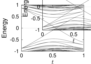
Figure 8: The energy eigenvalue spectrum in the vicinity of the band center for the kernel $D[\Delta(t)]$ from Eqs. (105d) and (119), is computed numerically as a function of the parameter $0\leq t\leq 1$ for $\left|\Delta^{\ }_{0}\right|/\Lambda=1$. The field $\Delta(t)$ interpolates between $\Delta^{\ }_{i}$ when $t=0$ and $\Delta^{\ }_{f}$ when $t=1$. Without loss of generality, the replica number $\mathsf{N}^{\ }_{\mathrm{r}}=1$ was chosen.

A.6 Summary

In summary, after integration over the Majorana spinors along the nearly-critical line of region CII in Fig. 4, the effective action for the Nambu-Goldstone field $\Delta$, a symmetric and unitary matrix, is given by

$$Z^{\mathrm{topolo}}_{\mathrm{NL}\sigma\mathrm{M}}=\int\mathcal{D}[\Delta]\,(-1)^{n[\Delta]}\,e^{-S[\Delta]}$$ (120a)

where $$S[\Delta] \sigma G/H=\mathrm{U}(2\mathsf{N}^{\ }_{\mathrm{r}})/\mathrm{O}(2\mathsf{N}^{\ }_{\mathrm{r}})$$ is the (fermionic replica version of the) action for the NLM on , i.e., Gade91-93

$$\begin{split}S[\Delta]=&\,\frac{1}{t^{\ }_{\mathrm{M}^{\prime}}}\int\mathrm{d}^{2}\,r\,\mathrm{tr}\left[\left(\partial^{\ }_{\mu}\Delta^{{\dagger}}\right)\left(\partial^{\ }_{\mu}\Delta\right)\right]\\ &\,+\frac{1}{t^{\ }_{a^{\prime}}}\int\mathrm{d}^{2}\,r\,\mathrm{tr}\left(\Delta^{{\dagger}}\partial^{\ }_{\mu}\Delta\right)\mathrm{tr}\left(\Delta\partial^{\ }_{\mu}\Delta^{{\dagger}}\right),\end{split}$$ (120b)

while

$$n[\Delta]=0,1$$ (120c)

– the $\mathbb{Z}^{\ }_{2}$-topological quantum number of $\Delta$ – reflects the ambiguity in defining globally the sign of the Pfaffian of Majorana spinors. Because of the block structure (115b), the topological quantum number $n[\Delta]=0,1$ is expected to survive the replica limit $\mathsf{N}^{\ }_{\mathrm{r}}\to 0$.

Appendix B Patterns of symmetry breaking and supermanifolds

There are 10 target spaces ${G}/{H}$ for the NL$\sigma$Ms of relevance to the 10 symmetry classes of Anderson localization. Zirnbauer96 ; Altland97 ; Heinzner05 They encode 10 distinct patterns of symmetry breaking. These patterns have been exhaustively classified within a supersymmetric approach by Zirnbauer in Ref. Zirnbauer96, . Each target superspace ${G}/{H}$ is a Riemannian symmetric supermanifold that can be parametrized in its bosonic sector by the Riemannian symmetric manifold

$${M}^{\ }_{B}={M}^{\ }_{BB}\times{M}^{\ }_{FF}.$$ (121)

Here, ${M}^{\ }_{B}$ is the direct product between a non-compact Riemannian symmetric manifold ${M}^{\ }_{BB}$ originating from the boson-boson sector of the Riemannian symmetric supermanifold and a compact Riemannian symmetric manifold ${M}^{\ }_{FF}$ originating from the fermion-fermion sector of the Riemannian symmetric supermanifold. The target superspaces ${G}/{H}$ and Riemannian symmetric manifolds ${M}^{\ }_{B}={M}^{\ }_{BB}\times{M}^{\ }_{FF}$ relevant to this paper are:

• ${G}/{H}=\mathrm{GL}(n|n)\times\mathrm{GL}(n|n)/\mathrm{GL}(n|n)=\mathrm{GL}(n|n)$ with the Riemannian symmetric manifolds

  $$\begin{split}&{M}^{\ }_{BB}=\mathrm{GL}(n,\mathbb{C})/\mathrm{U}(n),\\ &{M}^{\ }_{FF}=\mathrm{U}(n),\end{split}$$ (122)

  for the chiral symmetry class AIII,

• ${G}/{H}=\mathrm{GL}(2n|2n)/\mathrm{OSp}(2n|2n)$ with the Riemannian symmetric manifolds

  $$\begin{split}&{M}^{\ }_{BB}=\mathrm{GL}(2n,\mathbb{R})/\mathrm{O}(2n),\\ &{M}^{\ }_{FF}=\mathrm{U}(2n)/\mathrm{Sp}(2n),\end{split}$$ (123)

  for the chiral symmetry class BDI,

• ${G}/{H}=\mathrm{GL}(2n|2n)/\mathrm{OSp}(2n|2n)$ with the Riemannian symmetric manifolds

  $$\begin{split}&{M}^{\ }_{BB}=\mathrm{U}^{*}(2n)/\mathrm{Sp}(2n),\\ &{M}^{\ }_{FF}=\mathrm{U}(2n)/\mathrm{O}(2n),\end{split}$$ (124)

  for the chiral symmetry class CII,

• ${G}/{H}=\mathrm{OSp}(2n|2n)/\mathrm{GL}(n|n)$ with the Riemannian symmetric manifolds

  $$\begin{split}&{M}^{\ }_{BB}=\mathrm{Sp}(4n,\mathbb{R})/\mathrm{U}(n),\\ &{M}^{\ }_{FF}=\mathrm{O}(2n)/\mathrm{U}(n),\end{split}$$ (125)

  for the BdG symmetry class D,

• ${G}/{H}=\mathrm{OSp}(4n|4n)/\mathrm{OSp}(2n|2n)\times\mathrm{OSp}(2n|2n)$ with the Riemannian symmetric manifolds

  $$\begin{split}&{M}^{\ }_{BB}=\mathrm{Sp}(2n,2n)/\mathrm{Sp}(2n)\times\mathrm{Sp}(2n),\\ &{M}^{\ }_{FF}=\mathrm{SO}(4n)/\mathrm{SO}(2n)\times\mathrm{SO}(2n),\end{split}$$ (126)

  for the symplectic symmetry class AII.

The compatibility of these target superspaces with the addition of a topological term in the corresponding NL$\sigma$M is solely determined by the compact Riemannian symmetric manifold ${M}^{\ }_{FF}$: A topological term requires a non-trivial second homotopy group of ${M}^{\ }_{FF}$ (e.g., CII and AII). In this context, observe that the Riemannian symmetric supermanifolds for symmetry classes BDI and CII merely differ by the exchange of the boson-boson and fermion-fermion stabilizers $\mathrm{O}(2n)$ and $\mathrm{Sp}(2n)$ [in that regard, it is convenient to view $\mathrm{U}^{*}(2n)$ as a non-compact real subgroup of $\mathrm{GL}(2n,\mathbb{C})$]. This small difference is of great consequences since the NL$\sigma$M for the symmetric class BDI cannot be augmented by a topological term.

For simplicity, we consider symmetry class CII with $n=1$. According to Eq. (124), the target superspace is

$$\mathrm{GL}(2|2)/\mathrm{OSp}(2|2)\approx\mathrm{GL}(2|2)/\mathrm{SL}(1|2)$$ (127)

whereby we used the isomorphism $\mathrm{OSp}(2|2)\approx\mathrm{SL}(1|2)$. The projected CII target superspace obtained by quotienting out the two diagonal generators of $\mathrm{GL}(2|2)$ is

$$\mathrm{PSL}(2|2)/\mathrm{OSp}(2|2)\approx\mathrm{PSL}(2|2)/\mathrm{SL}(1|2).$$ (128a)

One must carry this projection on the non-compact and compact Riemannian symmetric manifolds (124). This is done by quotienting out their $$\mathbb{R}^{\ }_{+} \mathrm{U}(1)$$ and factors, respectively. Hence, the projected boson-boson Riemannian symmetric manifold is

$$\mathrm{SU}^{*}(2)/\mathrm{Sp}(2)\approx\mathrm{SU}^{*}(2)/\mathrm{SU}(2)$$ (128b)

while the projected fermion-fermion Riemannian symmetric manifold is

$$\mathrm{SU}(2)/\mathrm{O}(2)\sim S^{2}.$$ (128c)

Appendix C The supergroup $\mathrm{PSL}(n|n)$

Let $n\in\mathbb{N}$ be an integer and denote with $\mathrm{smat}(n|n)$ the set of all real $(n|n)$ supermatrices ${M}$, i.e., matrices of the form

$${M}:=\begin{pmatrix}{M}^{\ }_{BB}&{M}^{\ }_{BF}\\ {M}^{\ }_{FB}&{M}^{\ }_{FF}\end{pmatrix}$$ (129)

where ${M}^{\ }_{BB}$ and ${M}^{\ }_{FF}$ are $n\times n$ real-valued matrices while ${M}^{\ }_{BF}$ and ${M}^{\ }_{FB}$ are $n\times n$ Grassmann-valued matrices. We shall denote with $I$ and $J$ the $(n|n)$ diagonal supermatrices

$$\begin{split}&I:=\mathrm{diag}\begin{pmatrix}1&\cdots&1&1&\cdots&1\end{pmatrix},\\ &J:=\mathrm{diag}\begin{pmatrix}1&\cdots&1&-1&\cdots&-1\end{pmatrix},\end{split}$$ (130)

respectively. For any element ${M}\in\mathrm{smat}(n|n)$, the supertrace is defined by

$$\mathrm{str}\,{M}:=\mathrm{tr}\,{M}^{\ }_{BB}-\mathrm{tr}\,{M}^{\ }_{FF}.$$ (131)

Observe that

$$\begin{split}&\mathrm{tr}\,{M}^{\ }_{BB}=\frac{1}{2}\left(\mathrm{str}\,{MJ}+\mathrm{str}\,{MI}\right),\\ &\mathrm{tr}\,{M}^{\ }_{BF}=\frac{1}{2}\left(\mathrm{str}\,{MJ}-\mathrm{str}\,{MI}\right),\end{split}$$ (132)

i.e., demanding that $\mathrm{tr}\,{M}^{\ }_{BB}$ and $\mathrm{tr}\,{M}^{\ }_{BF}$ both vanish is equivalent to demanding that $\mathrm{str}\,{MJ}$ and $\mathrm{str}\,{MI}$ both vanish. For any element ${M}\in\mathrm{smat}(n|n)$ with $\mathrm{det}\,{M}^{-1}_{FF}\neq 0$ or $\mathrm{det}\,{M}^{-1}_{BB}\neq 0$ the superdeterminant is defined by

$$\mathrm{sdet}\,{M}:=\frac{\mathrm{det}\,\left({M}^{\ }_{BB}-{M}^{\ }_{BF}{M}^{-1}_{FF}{M}^{\ }_{FB}\right)}{\mathrm{det}\,{M}^{\ }_{FF}},$$ (133)

or

$$\mathrm{sdet}\,{M}:=\frac{\mathrm{det}\,\left({M}^{\ }_{FF}-{M}^{\ }_{FB}{M}^{-1}_{BB}{M}^{\ }_{BF}\right)}{\mathrm{det}\,{M}^{-1}_{BB}},$$ (134)

respectively.

An obvious generalization of $\mathrm{smat}(n|n)$ is achieved through the complexification

$${M}\to{M}+{i}{M}^{\prime},\qquad{M},{M}^{\prime}\in\mathrm{smat}(n|n).$$ (135)

Another one follows from the substitution

$$\mathrm{smat}(n|n)\to\mathrm{smat}(m|n)$$ (136)

where the supermatrices from the set $\mathrm{smat}(m|n)$ are of the form (129) with the entries of the $m\times m$ matrix ${M}^{\ }_{BB}$ and the $n\times n$ matrix ${M}^{\ }_{FF}$ commuting numbers while the entries of the the $m\times n$ matrix ${M}^{\ }_{BF}$ and the $n\times m$ matrix ${M}^{\ }_{FB}$ are anticommuting numbers.

The following definitions apply to both real and complex supermatrices. The supergroup $\mathrm{PSL}(n|n)$ is constructed from the supergroup $\mathrm{GL}(n|n)\subset\mathrm{smat}(n|n)$ as follows. The supergroup $\mathrm{GL}(n|n)$ consists of all $(n|n)$ supermatrices for which both ${M}^{\ }_{BB}$ and ${M}^{\ }_{FF}$ are non-singular (i.e., have nonvanishing determinants) and with the matrix multiplication as the group operation. The supergroup $\mathrm{GL}(n|n)$ is not semisimple. It possesses the matrix subsupergroup $\mathrm{SL}(n|n)$ that follows from restricting the superdeterminants in $\mathrm{GL}(n|n)$ to one. The supergroup $\mathrm{SL}(n|n)$ is also not semisimple, for it contains the $(n|n)$ unit supermatrix $I$ that commutes with all $(n|n)$ supermatrices. All elements of $\mathrm{SL}(n|n)$ are generated through exponentiation of elements of the Lie superalgebra $\mathrm{sl}(n|n)$ whereby any element of $\mathrm{sl}(n|n)$ is a $(n|n)$ supermatrix of the form

$${X}:=\begin{pmatrix}{X}^{\ }_{BB}&{X}^{\ }_{BF}\\ {X}^{\ }_{FB}&{X}^{\ }_{FF}\end{pmatrix}$$ (137)

with ${X}^{\ }_{BB}$ and ${X}^{\ }_{FF}$ $n\times n$ real-valued matrices while ${M}^{\ }_{BF}$ and ${M}^{\ }_{FB}$ are $n\times n$ Grassmann-valued matrices with the vanishing supertrace

$$\mathrm{str}\,{X}=0.$$ (138)

The supergroup $\mathrm{PSL}(n|n)$ is defined to be the factor group $\mathrm{SL}(n|n)/\mathbb{R}^{\ }_{+}$ ($\mathbb{R}^{\ }_{+}$ the set of positive real numbers) by which any two elements in $\mathrm{sl}(n|n)$ that differ by a multiple of the unit element $I$ generate upon exponentiation the very same element of $\mathrm{PSL}(n|n)$. The supergroup $\mathrm{PSL}(n|n)$ is semisimple, an element of $\mathrm{PSL}(n|n)$ cannot be written as a supermatrix.

Appendix D The Lie group U${}^{*}(2)$

Let $n\in\mathbb{N}$. The Lie group U${}^{*}(2n)$ is the set of matrices in GL$(2n,\mathbb{C})$ that commutes with the linear transformation

$$\psi:\mathbb{C}^{2n}\to\mathbb{C}^{2n},\begin{pmatrix}z^{\ }_{1}\\ \vdots\\ z^{\ }_{n}\\ z^{\ }_{n+1}\\ \vdots\\ z^{\ }_{2n}\end{pmatrix}\to\begin{pmatrix}z^{*}_{n+1}\\ \vdots\\ z^{*}_{2n}\\ -z^{*}_{1}\\ \vdots\\ -z^{\*}_{n}\end{pmatrix}$$ (139)

where complex conjugation is denoted by ^∗. It follows that the Lie algebra u${}^{*}(2n)$ is the set of matrices in GL$(2n,\mathbb{C})$ of the form

$$\begin{pmatrix}Z^{\ }_{1}&Z^{\ }_{2}\\ -Z^{*}_{2}&Z^{*}_{1}\end{pmatrix}$$ (140)

where $Z^{\ }_{1}$ and $Z^{\ }_{2}$ are any complex-valued $n\times n$ matrices.

We now specialize to the Lie group U${}^{*}(2)$ with the Lie algebra u${}^{*}(2)$. Let $X\in$u${}^{*}(2)$. There exist the complex numbers $z^{\ }_{1}$ and $z^{\ }_{2}$ such that

$$\begin{split}X=&\,\begin{pmatrix}z^{\ }_{1}&z^{\ }_{2}\\ -z^{*}_{2}&z^{*}_{1}\end{pmatrix}\\ =&\,\mathrm{Re}\,z^{\ }_{1}\,\sigma^{\ }_{0}+{i}\mathrm{Im}\,z^{\ }_{2}\,\sigma^{\ }_{1}+{i}\mathrm{Re}\,z^{\ }_{2}\,\sigma^{\ }_{2}+{i}\mathrm{Im}\,z^{\ }_{1}\,\sigma^{\ }_{3}.\end{split}$$ (141)

Here, we have introduced the unit $2\times 2$ matrix $\sigma^{\ }_{0}$ and the three Pauli matrices $(\sigma^{\ }_{1},\sigma^{\ }_{2},\sigma^{\ }_{3})$. Evidently, U${}^{*}(2)$ and GL$(1,\mathbb{R})\times$SU$(2)$ share the same Lie algebra,

$$\mathrm{u}^{*}(2)\approx\mathbb{R}\oplus\mathrm{su}(2).$$ (142)

Locally, one thus have the isomorphism

$$\mathrm{U}^{*}(2)\approx\mathbb{R}^{\ }_{+}\otimes\mathrm{SU}(2)$$ (143)

where $\mathbb{R}^{\ }_{+}$ is the set of positive real numbers.

Appendix E NL$\sigma$M on homogeneous target spaces versus NL$\sigma$M on symmetric target spaces

In this Appendix we briefly summarize a number of facts about NL$\sigma$M on target spaces which are homogeneous spaces $G/H$. (For more details we refer the reader, for example, to the appendix of footnote: homogeneous space, , and references therein.)

The essential properties of a NL$\sigma$M whose target space is of the form of a coset space $G/H$, where $G$ is a Lie group and $H$ a Lie-subgroup, are as follows.

If $H$ is a maximal subgroup of $G$, then the NL$\sigma$M has precisely one coupling constant (the target space $G/H$ is then what is known as a ‘symmetric space’). If, on the other hand, there exists precisely one intervening subgroup $H^{\prime}$, i.e.,

$$H\subset H^{\prime}\subset G,$$ (144)

then the NL$\sigma$M with target space $G/H$ turns out to have precisely two independent coupling constants. If, in the latter case, we were to run the RG into the infrared (i.e., to large length scales), then one of the two coupling constants will disappear. In this case one ends up, asymptotically at long scales, with a NL$\sigma$M with one coupling constant, whose target space will be either $G/H^{\prime}$ or $H^{\prime}/H$ (both are, by assumption, symmetric spaces in the sense of maximal subgroups). The number of coupling constants for a NL$\sigma$M on a homogeneous space with more intervening subgroups increases accordingly.

The relevance of the symmetric space NL$\sigma$M for the universal physics appearing at large length scales is thus simply a consequence of the RG. If we begin with a NL$\sigma$M on a general homogeneous space, the RG will select, asymptotically at long length scales, a target space which is a symmetric space $G/H$ where $H$ is a maximal subgroup of $G$. So, all NL$\sigma$M on coset spaces become NL$\sigma$M on symmetric spaces, asymptotically at long length scales. It is for this reason that they are the “stable” large-scale limits, and appear naturally, without fine-tuning.

The appearance of a NL$\sigma$M (on a, in general, possibly homogeneous and not necessarily symmetric space) arises in a physical context from the general principle of symmetry breaking. The group $G$ is the global symmetry group of the problem. The subgroup $H$ (not necessarily maximal) characterizes the symmetries which are preserved when the global symmetry $G$ is broken.

In the situation discussed in this article, the global symmetry group is

$$G=\mathrm{GL}(2m|2m),\qquad m=1,2,\cdots.$$ (145)

When a global density of states (DOS) is generated in the Dirac fermion formulation of the theory, the resulting expectation value breaks the symmetry $G$ but preserves the symmetry $H\subset G$. It follows from Ref. Guruswamy00, that on the “dotted line” in our global phase diagram in Fig. 4 this subgroup is ${H^{\prime}}=\mathrm{OSp}(2m|2m)$. The manifold $G/{H^{\prime}}=\mathrm{GL}(2m|2m)/\mathrm{OSp}(2m|2m)$ is the symmetric space corresponding to symmetry class CII. On the boundary of the CII region the symmetry class is AII, corresponding to a target manifold ${H^{\prime}}/H=\mathrm{OSp}(2m|2m)/[\mathrm{OSp}(m|m)\times\mathrm{OSp}(m|m)]$. Thus, the entire lower half of our global phase diagram in Fig. 4 can be described by the NL$\sigma$M on the homogeneous space

$$G/H=\mathrm{GL}(2m|2m)/[\mathrm{OSp}(m|m)\times\mathrm{OSp}(m|m)].$$ (146)

which has two coupling constants (besides the coupling of the Gade term). This is analogous to the discussion in footnote: homogeneous space, .

References

- (1) P. R. Wallace, Phys. Rev. 71, 622 (1947).
- (2) see, e.g.: K. G. Wilson, Quarks and strings on the lattice, in New Phenomena in Subnuclear Physics, ed A. Zichini, Plenum Press (New York 1975).
- (3) H. B. Nielsen and M. Ninomiya, Nucl. Phys. B 193, 173 (1981).
- (4) R. Jackiw and C. Rebbi, Phys. Rev. D 13, 3398 (1976).
- (5) W. P. Su, J. R. Schrieffer, and A. J. Heeger, Phys. Rev. Lett. 42, 1698 (1979).
- (6) C. G. Callan and J. A. Harvey, Nucl. Phys. B 250, 427 (1985).
- (7) E. Fradkin, E. Dagotto, and D. Boyanovsky, Phys. Rev. Lett. 57, 2967 (1986); Nucl. Phys. B285, 340 (1987).
- (8) P. W. Brouwer, E. Racine, A. Furusaki, Y. Hatsugai, Y. Morita, and C. Mudry, Phys. Rev. B 66, 014204 (2002) .
- (9) D. B. Kaplan, Phys. Lett. B 288, 342 (1992).
- (10) Karl Jansen, Phys. Rep. 273, 1 (1996).
- (11) A. P. Schnyder, S. Ryu, A. Furusaki, and A. W. W. Ludwig, Phys. Rev. B 78, 195125 (2008).
- (12) M. R. Zirnbauer, J. Math. Phys. 37, 4986 (1996).
- (13) A. Altland and M. R. Zirnbauer, Phys. Rev. B 55, 1142 (1997).
- (14) P. Heinzner, A. Huckleberry, and M. R. Zirnbauer, Commun. Math. Phys. 257, 725 (2005).
- (15) Alexei Kitaev, arXiv:0901.2686 and Advances in Theoretical Physics: Landau Memorial Conference, AIP Conf. Proc. No. 1134 (AIP, New York, 2009), p. 22.
- (16) M. Stone, C.-K. Chiu, and A. Roy, J. Phys. A 44, 045001 (2011).
- (17) Andreas P. Schnyder, Shinsei Ryu, Akira Furusaki, and Andreas W. W. Ludwig, arXiv:0905.2029 and Advances in Theoretical Physics: Landau Memorial Conference, AIP Conf. Proc. 1134 (AIP, New York, 2009), p 10.
- (18) Shinsei Ryu, Andreas Schnyder, Akira Furusaki, and Andreas Ludwig, New J. Phys. 12, 065010 (2010).
- (19) Shinsei Ryu, Joel E. Moore, and Andreas W. W. Ludwig, Phys. Rev. B 85, 045104 (2012.
- (20) F. Evers and A. D. Mirlin, Rev. Mod. Phys. 80, 1355 (2008).
- (21) E. Fradkin, Phys. Rev. B 33, 3257 (1986).
- (22) A. W. W. Ludwig, M. P. A. Fisher, R. Shankar, and G. Grinstein, Phys. Rev. B 50, 7526 (1994).
- (23) A. A. Nersesyan, A. M. Tsvelik, and F. Wenger, Nucl. Phys. B 438, 561 (1995).
- (24) Claudio de C. Chamon, Christopher Mudry, and Xiao-Gang Wen, Phys. Rev. B 53, 7638(R) (1996).
- (25) C. C. Chamon, C. Mudry, and X.-G. Wen, Phys. Rev. Lett. 77, 4194 (1996).
- (26) C. Mudry, C. Chamon, and X.-G. Wen, Nucl. Phys. B 466, 383 (1996).
- (27) C. Mudry and X.-G. Wen, Nucl. Phys. B 549, 613 (1999).
- (28) M. Bocquet, D. Serban, and M. R. Zirnbauer Nucl. Phys. B 578, 628 (2000).
- (29) A. W. W. Ludwig, arXiv:cond-mat/0012189.
- (30) M.J. Bhaseen J.-S. Caux, I. I. Kogan, and A. M. Tsvelik, Nucl. Phys. B 618, 465 (2001).
- (31) A. Altland, B. D. Simons, and M. R. Zirnbauer, Phys. Rep. 359, 283 (2002).
- (32) L. Fu and C. L. Kane, Phys. Rev. B 76, 045302 (2007).
- (33) D. Hsieh, D. Qian, L. Wray, Y. Xia, Y. Hor, R. J. Cava, and M. Z. Hasan, Nature 452, 970 (2008).
- (34) D. Hsieh, Y. Xia, L. Wray, D. Qian, A. Pal, J. H. Dil, F. Meier, J. Osterwalder, G. Bihlmayer, C. L. Kane, Y. S. Hor, R. J. Cava, and M. Z. Hasan, Science 323, 919 (2009).
- (35) H. Zhang, C.-X. Liu, X.-L. Qi, X. Dai, Z. Fang, and S-C. Zhang, Nature Phys. 5, 438 (2009).
- (36) Y. L. Chen, J. G. Analytis, J. H. Chu, Z. K. Liu, S.-K. Mo, X. L. Qi, H. J. Zhang, D. H. Lu, X. Dai, Z. Fang, S. C. Zhang, I. R. Fisher, Z. Hussain, and Z.-X. Shen, Science 325, 178 (2009).
- (37) Y. Xia, L. Wray, D. Qian, D. Hsieh, A. Pal, H. Lin, A. Bansil, D. Grauer, Y. Hor, R. Cava, and M. Hasan, Nature Phys. 5, 398 (2009).
- (38) H. Lin, R.S. Markiewicz, L.A. Wray, L. Fu, M.Z. Hasan, and A. Bansil, Phys. Rev. Lett. 105, 036404 (2010).
- (39) B. Yan, C-X. Liu, H-J. Zhang, C-Y. Yam, X-L. Qi, T. Frauenheim, and S-C. Zhang, Euro. Phys. Lett. 90, 37002 (2010).
- (40) Y. L. Chen, Z. K. Liu, J. G. Analytis, J.-H. Chu, H. J. Zhang, B. H. Yan, S.-K. Mo, R. G. Moore, D. H. Lu, I. R. Fisher, S. C. Zhang, Z. Hussain, and Z.-X. Shen, Phys. Rev. Lett. 105, 266401 (2010).
- (41) Paul Fendley in “Lecture at the NATO Advanced Study Institute/EC Summer School on New Theoretical Approaches to Strongly Correlated Systems”, Newton Institute, Cambridge, UK, April 10-20, 2000; arXiv:cond-mat/0006360.
- (42) P. Fendley, Phys. Rev. B 63, 104429 (2001).
- (43) H. Eichenherr and M. Forger, Nucl. Phys. B 155, 381 (1979); F. D. M. Haldane, Phys. Lett. 93A, 464 (1983) and Phys. Rev. Lett. 50, 1153 (1983).
- (44) J. Wess and B. Zumino, Phys. Lett. 37B, 95 (1971).
- (45) S. P. Novikov, Usp. Mat. Nauk. 37, 3 (1982).
- (46) E. Witten, Commun. Math. Phys. 92, 455 (1984).
- (47) A. M. M. Pruisken, Nucl. Phys. B 235, 277 (1984).
- (48) T. Senthil, Matthew P. A. Fisher, L. Balents, and C. Nayak, Phys. Rev. Lett. 81, 4704 (1998).
- (49) T. Senthil and M. P. A. Fisher, Phys. Rev. B 61, 9690 (2000).
- (50) P. M. Ostrovsky, I. V. Gornyi, and A. D. Mirlin, Phys. Rev. Lett. 98, 256801 (2007).
- (51) S. Ryu, C. Mudry, H. Obuse, and A. Furusaki, Phys. Rev. Lett. 99, 116601 (2007).
- (52) D. Bernard and A. LeClair, J. Phys A 35, 2555 (2002).
- (53) Pavan Hosur, Shinsei Ryu, and Ashvin Vishwanath, Phys. Rev. B 81, 045120 (2010).
- (54) Y. Hatsugai, X.-G. Wen, and M. Kohmoto, Phys. Rev. B 56, 1061 (1997).
- (55) S. Guruswamy, A. LeClair, and A. W. W. Ludwig, Nucl. Phys. B 583, 475 (2000).
- (56) C. Mudry, S. Ryu, and A. Furusaki, Phys. Rev. B 67, 064202 (2003).
- (57) P. M. Ostrovsky, I. V. Gornyi, and A. D. Mirlin, Phys. Rev. B 74, 235443 (2006).
- (58) S. Ryu, C. Mudry, A. Furusaki, and A. W. W. Ludwig, Phys. Rev. B 75, 205344 (2007).
- (59) S. Ryu, C. Mudry, A. Ludwig, and A. Furusaki, Nucl. Phys. B 839, 341 (2010).
- (60) A. H. Castro Neto, F. Guinea, N. M. R. Peres, K. S. Novoselov, and A. K. Geim, Rev. Mod. Phys. 81, 109 (2009).
- (61) P. A. Lee, T. M. Rice, and P. W. Anderson, Phys. Rev. Lett. 31, 462 (1973).
- (62) V. Mitev, T. Quella, and V. Schomerus, JHEP 0811, 086 (2008).
- (63) C. Candu and H. Saleur, Nucl. Phys. B 808, 441 and 487 (2009).
- (64) C. Candu, V. Mitev, T. Quella, H. Saleur and V. Schomerus, JHEP 1002, 015 (2010).
- (65) Constantin Candu and Volker Schomerus, Phys. Rev. D 84, 051704 (2011).
- (66) J. H. Bardarson, J. Tworzydlo, P. W. Brouwer, and C. W. J. Beenakker, Phys. Rev. Lett. 99, 106801 (2007).
- (67) K. Nomura, M. Koshino, and S. Ryu, Phys. Rev. Lett. 99, 146806 (2007).
- (68) See also, A. P. Schnyder, C. Mudry, and I. A. Gruzberg, Nucl. Phys. B 822, 424 (2009).
- (69) V. S. Dotsenko and V. S. Dotsenko, Adv. Phys. 32, 129 (1983).
- (70) A. W. W. Ludwig, Nucl. Phys. B 285, 97 (1987).
- (71) R. Shankar, Phys. Rev. Lett. 58, 2466 (1987).
- (72) H. Obuse, A. R. Subramaniam, A. Furusaki, I. A. Gruzberg, and A. W. W. Ludwig, Phys. Rev. Lett. 101, 116802 (2008).
- (73) T. Quella, V. Schomerus, and T. Creutzig, JHEP 10, 024 (2008).
- (74) S. V. Morozov, K. S. Novoselov, M. I. Katsnelson, F. Schedin, L. A. Ponomarenko, D. Jiang, and A. K. Geim, Phys. Rev. Lett. 97, 016801 (2006); A. F. Morpurgo and F. Guinea, Phys. Rev. Lett. 97, 196804 (2006).
- (75) C.-Y. Hou, C. Chamon, and C. Mudry, Phys. Rev. Lett. 98, 186809 (2007).
- (76) E. Fradkin, Field Theories of Condensed Matter Systems, Addison-Wesley, Redwood City, CA (1991).
- (77) S. Ryu, A. Furusaki, A. W. W. Ludwig, and C. Mudry, Nucl. Phys. B 780, 105 (2007).
- (78) The analysis made in Ref. Ryu07b, applies to the case (50) or (52) although the corresponding Hamiltonian in this paper is in twice as large a representation of the Dirac equation than in Ref. Ryu07b, . Indeed, the chiral symmetry at the band center here implies that there is no need to distinguish retarded from advanced Green’s functions and thus to add another two-dimensional subspace for that purpose. There is no chiral symmetry in Ref. Ryu07b, so that the representation of the Dirac Hamiltonian in Ref. Ryu07b, must be doubled to account for the product of a pair of retarded and advanced Green’s functions.
- (79) Such a type of RG flow from a free Dirac state to a metallic state had been conjectured by M. Bocquet, D. Serban, and M. R. Zirnbauer in Ref. Bocquet00, . However, in that work the symmetry class in which this flow takes place was misidentified as class D, as opposed to the correct class AII. Moreover, the presence of a topological term on the sigma model side of the flow was overlooked. The latter is absolutely crucial, and was correctly identified in the recent works, Refs. Ostrovsky07, and Ryu07b, .
- (80) See, for our conventions of graded objects, Ref. Ryu06a, and references therein.
- (81) Here, we are using the conventions from Ref. Mudry03, for the normalization of the variances and for the normalization of the integration variables in the path integral (28). Be aware that the beta function in Eq. (5.2) from Ref. Mudry03, , contains a typographical error: The right-hand side of Eq. (5.2) from Ref. Mudry03, should be multiplied by . (The same beta function is denoted by in the present paper.)
-
(82)
The relevant RG flows can be derived from the
3 coupled perturbative RG flows computed by
D. Bernard, in
Low Dimensional Applications of Quantum field Theory,
edited by L. Baulieu et al.,
Vol. 362 of NATO Advanced Study Series B:Physics
(Plenum Press, New York, 1997),
for the random Hamiltonian
with the static random vector potential (variance ), the static scalar potential (variance ), and the static random mass (variance ). With our normalization conventions, the RG flows are
The stability of the vertical dotted line in region BDI of Fig. 4 follows from the analytical continuation , , and of these flows, as pointed out in Ref. Hatsugai97, . Similarly, the stability of the vertical dotted line in region CII of Fig. 4 follows from the analytical continuation , , and of these flows. -
(83)
Observe that does not flow along the
BDI boundaries
or the CII boundaries .
The projected slope in region BDI is
in Fig. 4(b). The projected slope in region CII is
in Fig. 4(b). Given these finite slopes of the flows out of the boundaries of regions BDI and CII, the reader might conclude that it is possible to flow from the region AIII to the regions BDI or CII. This is not so, however, as any pair of couplings and ( and ) or and ( and ) in region AIII always generates a flow to strong coupling of the variance associated to the vector gauge potentials that break time-reversal symmetry, see Eq. (4.84) from Ref. Guruswamy00, . These flows thus escape the regions BDI and CII for which . - (84) See Eq. (4.20) from Ref. Guruswamy00, or Eq. (5.7) from Ref. Mudry03, .
- (85) M. Bershadsky, S. Zhukov, and A. Vaintrob, Nucl. Phys. B 559, 205 (1999).
- (86) N. Berkovits, C. Vafa, and E. Witten, JHEP 9903, 018 (1999).
- (87) R. Gade, Nucl. Phys. B 398, 499 (1993); R. Gade and F. Wegner, ibid. 360, 213 (1991).
- (88) A detailed study of models can be found in N. Read and H. Saleur, Nucl. Phys. B 613, 409 (2001).
- (89) See, e.g., A. T. Lundell, Lect. Notes Math. 1509, 250 (1992).
- (90) I. Affleck and F. D. M. Haldane, Phys. Rev. B 36, 5291 (1987).
- (91) A. B. Zamolodchikov and Al. B. Zamolodchikov, Nucl. Phys. B 379, 602 (1992).
- (92) Ilya A. Gruzberg, Andreas W. W. Ludwig, and N. Read, Phys. Rev. Lett. 82, 4524 (1999).
-
(93)
Such a symmetry-breaking potential can be
chosen to be
where and is the fundamental (super) matrix field of the -WZNW model (and principal chiral model), which is a (super) matrix, arranged in four blocks of matrices as
Here, matrix elements are all bosonic for and , and all fermionic for and . This potential breaks the symmetry of the -WZNW model down to the diagonal symmetry group. Moreover, for any value of the coupling constant of the principal chiral model, this potential is a relevant perturbation. In particular, at weak coupling it is strongly relevant since the scaling dimension of the fundamental matrix field is close to zero. Consider the weakly coupled -principal chiral model, where the coupling constant of the potential grows large very rapidly. For very large values of only the configurations of the matrix field that minimize the potential(149)
will contribute to the functional integral. The matrix elements of and are fermionic, and vanish at the minimum of the potential. In terms of the eigenvalues of and the eigenvalues of , the potential in the absence of fermionic coordinates reads
Then the minimum occurs at , and . The matrix field
that minimizes the potential is thus invariant under conjugation by the subgroup of the bosonic part of the symmetry. Therefore, the addition of the relevant potential perturbation to the action reduces the target space of the principle chiral model to the target space of the NLM in symmetry class CII. At the same time, the WZ term reduces to a theta term at in the NLM. - (94) A. Hüffmann, J. Phys. A 23, 5733 (1990).
- (95) P. W. Brouwer, C. Mudry, and A. Furusaki, Nucl. Phys. B 565, 653 (2000).
- (96) C. Mudry, P. W. Brouwer, and A. Furusaki, Phys. Rev. B 62, 8249 (2000).
- (97) M. Titov, P. W. Brouwer, A. Furusaki, and C. Mudry, Phys. Rev. B 63, 235318 (2001).
- (98) P. W. Brouwer, A. Furusaki, and C. Mudry, Phys. Rev. B 67, 014530 (2003).
- (99) P. W. Brouwer, A. Furusaki, C. Mudry, and S. Ryu, BUTSURI 60, 935 (2005); arXiv:cond-mat/0511622.
- (100) P. W. Brouwer, C. Mudry, B. D. Simons, and A. Altland, Phys. Rev. Lett. 81, 862 (1998).
- (101) M. R. Zirnbauer, Phys. Rev. Lett. 69, 1584 (1992); A. D. Mirlin, A. Müller-Groeling, and M. R. Zirnbauer, Ann. Phys. (N.Y.) 236, 325 (1994).
- (102) Y. Takane, J. Phys. Soc. Jpn. 73, 9 (2004); 73, 1430 (2004); 73, 2366 (2004).
- (103) H. Obuse, A. Furusaki, S. Ryu, and C. Mudry, Phys. Rev. B 76, 075301 (2007).
- (104) A. P. Schnyder, S. Ryu, and A. W. W. Ludwig, Phys. Rev. Lett. 102, 196804 (2009).
- (105) D. H. Friedan, Ann. Phys. (N.Y.) 163, 318 (1985).
- (106) Ilya A. Gruzberg, N. Read, and Andreas W. W. Ludwig, Phys. Rev. B 63, 104422 (2001). (We direct the reader to Appendix E of this paper.)
- (107) O. Motrunich, K. Damle, and D. A. Huse, Phys. Rev. B 65, 064206 (2002).
- (108) Z. Ringel, Y. E. Kraus, and A. Stern, arXiv:1105.4351.
- (109) Roger S. K. Mong, Jens H. Bardarson, and Joel E. Moore, Phys. Rev. Lett. 108, 076804 (2012).
- (110) K. B. Efetov, A. I. Larkin, and D. E. Khemlnitskii, Sov. Phys. JETP 52, 568 (1980).
- (111) E. J. Weinberg, D. London, and J. L. Rosner, Nucl. Phys. B 236, 90 (1984).