Scattering of Dirac electrons by circular mass barriers: valley filter and resonant scattering

Abstract

The scattering of two-dimensional (2D) massless Dirac electrons is investigated in the presence of a random array of circular mass barriers. The inverse momentum relaxation time and the Hall factor are calculated and used to obtain parallel and perpendicular resistivity components within linear transport theory. We found a non zero perpendicular resistivity component which has opposite sign for electrons in the different $K$ and $K^{\prime}$ valleys. This property can be used for valley filter purposes. The total cross-section for scattering on penetrable barriers exhibit resonances due to the presence of quasi-bound states in the barriers that show up as sharp gaps in the cross-section while for Schrödinger electrons they appear as peaks.

I Introduction

Nanostructures have become the system of choice for studying transport over the past few yearsFerry . Starting with 2D (two dimensional) electron systems at the interface of two different materials several decades agoN0 , recently it has shifted to 2D relativistic materials e. g. graphene nov05 ; zang05 ; Nori1 and topological insulatorsmoo10 ; Hasan . In pristine graphene the conduction and valence bands touch each other in six points of the Brillouin zone and are defined by two independent sets of cones commonly called $K$ and $K^{\prime}$. Near these points the electronic dispersion is linear which corresponds to the dispersion of massless relativistic particles, described by the Dirac-Weyl equationsemenof ; wall47 .

During the last decades there has been a lot of theoretical and experimental attempts to use the spin of the electron as a carrier of informationWolf . Graphene in addition to the spin of the electron has two more degrees of freedom, sublattice pseudospin and valley isospin or valley index. In order to scatter an electron from the $K$ valley to the $K^{\prime}$ valley a large transfer of momentum is needed. Typical disorder and Coulomb-type of scattering is unable to provide this momentum and in such a case the valley isospin is a conserved quantum number in electronic transport. This allows us to use valley isospin as a carrier of information. It was shown that graphene nanoribbons with zigzag edgesbeen1 can be used as a valley filter. Another promising possibility to control the valley index of electrons is by using line defectsmass3 . These can be formed in graphene when grown on a Nickel substrate or by using so called mass barriers that can be created by proper arrangement of dopants in the graphene sheetmass1 ; mass2 .

The purpose of this work is to apply the above mentioned ideas to electron transport in the presence of circular mass barriers. We solve the Dirac electron scattering problem on a sharp circular mass barrier and calculated the cross-section, the inverse momentum relaxation time and the probability for the electron to be reflected in the perpendicular direction. In spite of the circular symmetry of the scatterers we obtain a non zero perpendicular component of resistivity that allows us to separate electrons with different chirality, or belonging to $K$ and $K^{\prime}$ valleys. The scattering of Dirac electrons by a penetrable circular mass barrier is influenced by the presence of quasi-bound states that results in resonant behavior. The obtained results are compared with those for standard Schrödinger electrons.

The paper is organized as follows. In section II we introduce the problem and illustrate our formalism by considering first the more simple problem of Dirac electrons scattered by a circular hole. In section III the boundary condition is obtained for a circular barrier i. e. a mass dot and a mass anti-dot. The bound states in the mass dot are calculated in section IV. In section V the scattering by an impenetrable circle is considered and the total cross section, relaxation time and Hall component of the resistivity is obtained. In section VI we repeat this calculation for a penetrable circle and compared the results with the results for standard electrons that are presented in Appendix A. Our conclusions are presented in section VII.

II Problem

We consider a Dirac electron interacting with circular barrier structures shown in Fig. 1 by the shadowed regions.

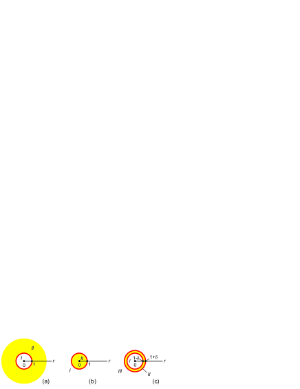
Figure 1: (Color online) Layout of the mass barrier profile: (a) – dot, (b) – anti-dot, and (c) – penetrable circle, i. e  a ring shaped barrier.

In the long wave approximation it is described by the stationary equation

$$\left\{H-E\right\}\Psi=0$$ (1)

with the following Dirac Hamiltonian:

$$H_{D}=\begin{pmatrix}\boldsymbol{\sigma}\cdot{\bf p}+\kappa\sigma_{z}&0\\ 0&\boldsymbol{\sigma}^{*}\cdot{\bf p}-\kappa^{\prime}\sigma_{z}\end{pmatrix}.$$ (2)

This $4\times 4$ matrix Hamiltonian describes low energy excitations in $K$ and $K^{\prime}$ valleys. Due to its diagonal form it is possible to separate the scattering problems in each $K$ or $K^{\prime}$ valley. We choose the following $2\times 2$ Hamiltonians:

$$H = \boldsymbol{\sigma}\cdot{\bf p}+\kappa({\bf r})\sigma_{z},$$ (3a)

$$H^{\prime} = \boldsymbol{\sigma}^{*}\cdot{\bf p}-\kappa^{\prime}({\bf r})\sigma_{z},$$ (3b)

where $\boldsymbol{\sigma}=\{\sigma_{x},\sigma_{y}\}$ and $\sigma_{z}$ stand for the Pauli matrices, and $\kappa,({\bf r}),\,\kappa^{\prime}({\bf r})$ characterizes the mass barrier for $K$ and $K^{\prime}$ electrons, respectively. We use dimensionless variables where velocities are measured in Fermi velocity unit $v_{F}$, all coordinates are measured in the radius $R$ of the circular scattering barrier, shown in Fig. 1 by the solid red line, and the electron energy — in $\hbar v_{F}/R$ units. From now on all equations are for $K$ valley electrons, except if otherwise specified.

According to standard scattering theory we present the wave function as

$$\Psi=\frac{1}{\sqrt{2}}\begin{pmatrix}1\\ 1\end{pmatrix}e^{iEx}+\frac{f(\varphi)}{\sqrt{r}}e^{iEr},$$ (4)

consisting on the incident wave in the $x$-direction and the scattered part. The scattered part is characterized by the two component scattering amplitude

$$f(\varphi)=\begin{pmatrix}A\\ B\end{pmatrix}.$$ (5)

As the incoming wave function part is normalized to unit flow density the differential cross-section is equal to the radial flow of electrons corresponding to the scattered wave function part, namely,

$$\sigma(\varphi)=f^{+}(\varphi)\left(\boldsymbol{\sigma}\cdot{\bf n}\right)f(\varphi)=\mathrm{e}^{i\varphi}AB^{*}+\mathrm{e}^{-i\varphi}A^{*}B,$$ (6)

where ${\bf n}=(\cos\varphi,\sin\varphi)$ is the unit vector in the considered direction.

Besides the above differential cross-section we shall consider the total cross-section

$$\sigma=\int_{0}^{2\pi}d\varphi\sigma(\varphi),$$ (7)

and two more averages: the inverse electron momentum relaxation time (the quantity proportional to the dissipative component of resistivity)

$$\gamma=\int_{0}^{2\pi}d\varphi\sigma(\varphi)\left(1-\cos\varphi\right),$$ (8)

and the quantity

$$\eta=\int_{0}^{2\pi}d\varphi\sigma(\varphi)\sin\varphi,$$ (9)

that corresponds to the perpendicular component of resistivity (or the analog of the Hall component in the case with magnetic field).

Due to the azimuthal symmetry of our problems it is convenient to use polar coordinates. Thus, assuming the total wave function as

$$\Psi({\bf r})=\begin{pmatrix}U({\bf r})\\ V({\bf r})\end{pmatrix},$$ (10)

we shall solve the set of equations

$$e^{-\mathrm{i}\varphi}\left(\frac{\partial}{\partial r}-\frac{\mathrm{i}}{r}\frac{\partial}{\partial\varphi}\right)V = \mathrm{i}(E-\kappa)U,$$ (11a)

$$e^{\mathrm{i}\varphi}\left(\frac{\partial}{\partial r}+\frac{\mathrm{i}}{r}\frac{\partial}{\partial\varphi}\right)U = \mathrm{i}(E+\kappa)V$$ (11b)

for the wave function components.

Now we expand the wave function into partial waves

$$\begin{pmatrix}U({\bf r})\\ V({\bf r})\end{pmatrix}=\sum_{m=-\infty}^{\infty}w_{m}e^{im\varphi}\begin{pmatrix}u_{m}(r)\\ ie^{i\varphi}v_{m}(r)\end{pmatrix},$$ (12)

replacing Eqs. (11) by the following set of two radial equations:

$$\left(\frac{d}{dr}+\frac{m+1}{r}\right)v_{m} = (E-\kappa)u_{m},$$ (13a)

$$\left(\frac{d}{dr}-\frac{m}{r}\right)u_{m} = -(\kappa+E)v_{m}.$$ (13b)

These equations are our main instrument when considering the problems shown in Fig. 1.

III Boundary conditions

For the sake of simplicity we restrict ourselves to model problems with large mass potentials, and replace the potentials by proper boundary conditions on the electron wave functions. In fact, this is the standard way of describing low energy scattering. For this purpose we have to solve the appropriate equations in the barrier region, to apply the standard boundary conditions for both wave function components on the solid circles shown in Fig. 1, and to calculate the limit $\kappa\to\infty$. We start with the system shown in Fig. 1(c). Thus, we have to solve the following approximate set of radial equations:

$$\frac{d}{dr}v = -\kappa u,$$ (14a)

$$\frac{d}{dr}u = -\kappa v$$ (14b)

in the thin shadowed region $II$ which is delimited by two circles of radius $1\pm\delta$ ($\delta\ll 1$). Its solution reads

$$u = Fe^{\kappa(r-1)}+Ge^{-\kappa(r-1)},$$ (15a)

$$v = -Fe^{\kappa(r-1)}+Ge^{-\kappa(r-1)}.$$ (15b)

Now satisfying the boundary conditions on the two circles demarcating the region $II$ we obtain the following set of four algebraic equations

$$u_{I}(1-\delta) = F\mathrm{e}^{-\kappa\delta}+G\mathrm{e}^{\kappa\delta},$$ (16a)

$$v_{I}(1-\delta) = -F\mathrm{e}^{-\kappa\delta}+G\mathrm{e}^{\kappa\delta},$$ (16b)

$$u_{III}(1+\delta) = F\mathrm{e}^{\kappa\delta}+G\mathrm{e}^{-\kappa\delta},$$ (16c)

$$v_{III}(1+\delta) = -F\mathrm{e}^{\kappa\delta}+G\mathrm{e}^{-\kappa\delta}.$$ (16d)

Eliminating the coefficients $F$ and $G$ we obtain in the limit $\delta\ll 1$ the boundary conditions

$$v_{III}(1)-v_{I}(1) = -\left\{u_{III}(1)+u_{I}(1)\right\}\tanh(\kappa\delta),\phantom{mmu}$$ (17a)

$$u_{III}(1)-u_{I}(1) = -\left\{v_{III}(1)+v_{I}(1)\right\}\tanh(\kappa\delta),$$ (17b)

connecting wave function components in the regions $I$ and $III$.

For a very thin and very high mass barrier (the analog of $\delta$-type barrier for Schrödinger electrons, see Sec. A) we take the following limits:

$$\delta\to 0,\quad\kappa\to\infty,\quad\tanh(\kappa\delta)=P=\mathrm{const},$$ (18)

what enables us to rewrite Eqs. (17) as

$$v_{III}(1)-v_{I}(1) = -P\left\{u_{III}(1)+u_{I}(1)\right\},$$ (19a)

$$u_{III}(1)-u_{I}(1) = -P\left\{v_{III}(1)+v_{I}(1)\right\}.$$ (19b)

These boundary conditions can be formally replaced by inserting Dirac $\delta$-functions into Eqs. (13), namely, replacing those equations by

$$\left(\frac{d}{dr}+\frac{m+1}{r}\right)v_{m} = \left[E-2P\delta(r-1)\right]u_{m},$$ (20a)

$$\left(\frac{d}{dr}-\frac{m}{r}\right)u_{m} = -\left[2P\delta(r-1)+E\right]v_{m},\phantom{mm}$$ (20b)

if we assume the following rule for calculating the integrals when the integrand is a product of Dirac $\delta$-function and some function $f(x)$ with the discontinuityroy93 :

$$\lim_{\alpha\to+0}\int_{-\alpha}^{\alpha}dx\delta(x)f(x)=\frac{1}{2}\left\{f(+0)+f(-0)\right\}.$$ (21)

The parameter $P$ characterizes the effective strength of the $\delta$-type barrier, and never exceeds the value $P=1$ in contrast to the case of Schrödinger electrons where it can take any value. A second major difference is that the wave function components $u(r)$ and $v(r)$ are discontinuous at the position of the $\delta$-function (but the probability density is continuous) while for Schrödinger electrons the wave function is continuous but the derivative of the wave function is discontinuous in that position. This is a consequense of the fact that the Dirac-Weyl equation is a first order diferential equation while the Schrödinger equation is second order.

The obtained boundary conditions for the general case shown in Fig. 1(c) enables us to construct analogous boundary conditions for the two other cases shown by Figs. 1(a,b). So, in the case of Fig. 1(a) we assume

$$\kappa=\infty,\quad P=1,\quad u_{III}(1)=v_{III}(1)=0,$$ (22)

and rewrite the boundary conditions given by Eqs. (19) as

$$u_{I}(1)=v_{I}(1).$$ (23)

This is the boundary condition for the quantum dot, surrounded by an infinite mass barrier.

In the case of Fig. 1(b) an analogous reasoning leads to the following boundary condition:

$$u_{I}(1)=-v_{I}(1),$$ (24)

that we shall use for describing Dirac electron scattering by a hard wall anti-dot.

The obtained boundary conditions enables us to neglect the $\kappa$ terms in Eqs. (13) and solve the Dirac equations for free electrons

$$\left(\frac{d}{dr}+\frac{m+1}{r}\right)v_{m} = Eu_{m},$$ (25a)

$$\left(\frac{d}{dr}-\frac{m}{r}\right)u_{m} = -Ev_{m}$$ (25b)

in regions $I$ and $III$ separately.

IV Bound states in the dot

The most simple problem is the one of a quantum dot shown in Fig. 1(a). In this case the solution of Eqs. (25) in region $I$ has to be finite at $r=0$ and is given by Bessel functions

$$u(r) = FJ_{m}(Er),$$ (26a)

$$v(r) = FJ_{m+1}(Er).$$ (26b)

Satisfying boundary condition (23) we immediately arrive at the algebraic equation

$$J_{m}(E)-J_{m+1}(E)=0$$ (27)

that determines the energy of the bound states.

V Scattering by an impenetrable circle

Now we shall consider our main problems, namely, the scattering of Dirac electrons by circular mass barriers. We shall start with the case presented in Fig. 1(b) — the scattering by an impenetrable circle (or by a hard wall anti-dot). According to standard scattering theory we have to construct the total wave function (10) solving the Dirac equations for free electrons (25) in the outer region $I$ that satisfies the boundary condition (24), to exclude the incoming part of the wave function, and calculate the cross-section by means of Eq. (6).

So, the solution of Eqs. (25) in the outer region $I$ reads

$$u_{m}(r)=w_{m}\left[J_{m}(Er)\cos\delta_{m}+Y_{m}(Er)\sin\delta_{m}\right],\phantom{mmmm}$$ (28a)

$$v_{m}(r)=w_{m}\left[J_{m+1}(Er)\cos\delta_{m}+Y_{m+1}(Er)\sin\delta_{m}\right].\phantom{mm}$$ (28b)

where the symbols $J_{m}$ and $Y_{m}$ stand for Bessel and Neumann functions, respectively.

Now satisfying the boundary conditions (24) for any partial wave function harmonic individually we obtain the expansion coefficients $\sin\delta_{m}$ and $\cos\delta_{m}$ through the so called phase shifts

$$\tan\delta_{m}=-\frac{J_{m}(E)+J_{m+1}(E)}{Y_{m}(E)+Y_{m+1}(E)}.$$ (29)

Usually the exclusion of the incoming plane wave from the total wave function (12) is done in the asymptotic region where $Er\gg 1$. Here we use the asymptotic of the Bessel functions $J_{m}(Er)\approx\sqrt{2/\pi Er}\cos\Delta_{m}$, $Y_{m}(Er)\approx\sqrt{2/\pi Er}\sin\Delta_{m}$ where

$$\Delta_{m}=Er-\frac{\pi}{2}m-\frac{\pi}{4},$$ (30)

which allows us to write the total wave function components as

$$U(\bi{r}) = \sqrt{\frac{2}{\pi kr}}\sum_{m=-\infty}^{\infty}w_{m}e^{im\varphi}\cos(\Delta_{m}-\delta_{m}),$$ (31a)

$$V(\bi{r}) = i\sqrt{\frac{2}{\pi kr}}\sum_{m=-\infty}^{\infty}w_{m}e^{i(m+1)\varphi}\cos(\Delta_{m+1}-\delta_{m}).\phantom{mmm}$$ (31b)

In this asymptotic region the incoming plane wave can be presented as

$$\begin{split}\mathrm{e}^{iEx}&=\sum_{m=-\infty}^{\infty}i^{m}e^{im\varphi}J_{m}(Er)\\ &\approx\sqrt{\frac{2}{\pi Er}}\sum_{m=-\infty}^{\infty}i^{m}e^{im\varphi}\cos\Delta_{m}\\ &=\sqrt{\frac{1}{2\pi Er}}\sum_{m=-\infty}^{\infty}i^{m}e^{im\varphi}\left(e^{i\Delta_{m}}+e^{-i\Delta_{m}}\right).\end{split}$$ (32)

Now in order to compensate the incoming term in the total wave function (12) by the second term of the last line in Eq. (32) we have to take

$$w_{m}=\frac{1}{\sqrt{2}}i^{m}e^{-i\delta_{m}}.$$ (33)

It is remarkable that this choice makes the above mentioned compensation in both scattering amplitude components $A$ and $B$, but not in every pair of radial components $u_{m}$ and $v_{m}$ separately. This is related to the fact that the angular momentum is not conserved quantity but that the Dirac-Weyl Hamiltonian commutes with operator consisting of the angular momentum plus isospin. So, inserting the above expression of $w_{m}$ into Eq. (31) and subtracting the incoming wave function part given by Eq. (32) we arrive after laborious but straightforward calculations at the following expression for the components of the scattering amplitude (5):

$$A = e^{-3i\pi/4}\sqrt{\frac{1}{\pi E}}\sum_{m=-\infty}^{\infty}e^{im\varphi}e^{-i\delta_{m}}\sin\delta_{m},$$ (34a)

$$B = e^{-3i\pi/4}e^{i\varphi}\sqrt{\frac{1}{\pi E}}\sum_{m=-\infty}^{\infty}e^{im\varphi}e^{-i\delta_{m}}\sin\delta_{m}.\phantom{mm}$$ (34b)

Inserting them into Eq. (6) we obtain the following differential cross-section:

$$\sigma(\varphi)=\frac{2}{\pi E}\sum_{m,m^{\prime}=-\infty}^{\infty}e^{i\left[(m-m^{\prime})\varphi-(\delta_{m}-\delta_{m^{\prime}})\right]}\sin\delta_{m}\sin\delta_{m^{\prime}}.$$ (35)

We have to keep in mind that the derivation of this cross-section was performed with the Hamiltonian (3a), which is valid for electrons in the $K$ valley.

To obtain the results for $K^{\prime}$ valley electrons we have to repeat the procedure starting with Hamiltonian (3b). Fortunately, it leads to the same set of differential equations (11) with a single change $U\rightleftarrows V$. Further, we replace Eq. (12) by

$$\begin{pmatrix}U({\bf r})\\ V({\bf r})\end{pmatrix}=\sum_{m=-\infty}^{\infty}w_{m}e^{-im\varphi}\begin{pmatrix}u_{m}(r)\\ -ie^{-i\varphi}v_{m}(r)\end{pmatrix},$$ (36)

and arrive at the same radial equation set (13) as was obtained for the $K$ valley case. Consequently, all equations, including the boundary condition, remain the same for the $K^{\prime}$ valley as well. The equation for the differential cross-section for the $K^{\prime}$ valley, however, differs. In this case the changes $m\to-m$ and $m^{\prime}\to-m^{\prime}$ have to be performed in the argument of the exponent leaving the same indexes of phase shifts $\delta_{m}$ and $\delta_{m^{\prime}}$.

Now inserting the obtained differential cross-section (35) into Eq. (7) we obtain the total cross-section

$$\begin{split}\sigma&=\frac{4}{E}\sum_{m,m^{\prime}=-\infty}^{\infty}\delta_{m,m^{\prime}}e^{i(\delta_{m^{\prime}}-\delta_{m})}\sin\delta_{m}\sin\delta_{m^{\prime}}\\ &=\frac{4}{E}\sum_{m=-\infty}^{\infty}\sin^{2}\delta_{m}.\end{split}$$ (37)

Note the above mentioned change $m\to-m$ and $m^{\prime}\to-m^{\prime}$ in the exponent argument now appears as the same change in the argument of the Kronecker symbol $\delta_{m,m^{\prime}}$. It is evident that this change does not influence the total cross-section, and consequently, it is the same for both $K$ and $K^{\prime}$ valley electrons.

Taking into account Eq. (29) the partial cross-section contribution to the total cross-section can be presented as

$$\begin{split}&\sin^{2}\delta_{m}\\ &=\frac{\left[J_{m}(E)+J_{m+1}(E)\right]^{2}}{\left[J_{m}(E)+J_{m+1}(E)\right]^{2}+\left[Y_{m}(E)+Y_{m+1}(E)\right]^{2}},\end{split}$$ (38)

what enables us to calculate the scattering cross-section directly.

The energy dependence of the total cross-section where the sum is restricted by the value $M$ ($|m|\leqslant M$) is shown in Fig. 2.

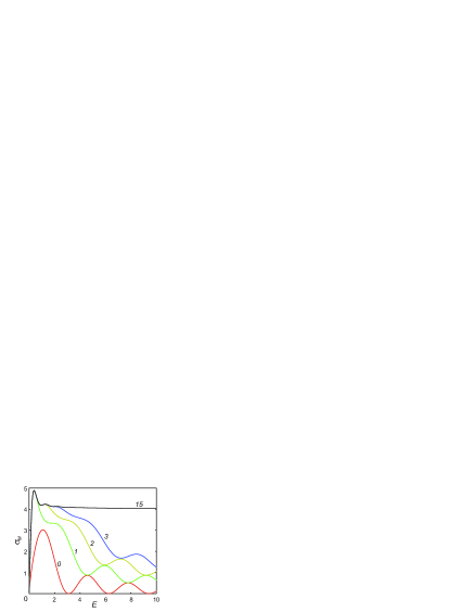
Figure 2: (Color online) The energy dependence of the partial sums $\sigma_{M}$ contributing to the total cross-section. The italic numbers on the curves indicate the number $M$. The black curve for $M=15$ corresponds to the convergent result.

We see a rather good convergence at low energies where three terms (i. e. $m=0,\pm 1$) are already sufficient.

The oscillating behavior of the energy dependence of the partial sum follows from the same behavior of the separate terms in Eq. (37) that can be easily explained calculating the asymptotic of the phase shifts. Indeed, using the asymptotic of the Bessel functions and replacing $\Delta_{m}$ by $\Delta_{m}|_{r=1}$ we have the following asymptotic expression for the scattering phase (29):

$$\begin{split}\tan\delta_{m}&=-\frac{J_{m}(E)+J_{m+1}(E)}{Y_{m}(E)+Y_{m+1}(E)}\approx\frac{\cos\Delta_{m}+\cos\Delta_{m+1}}{\sin\Delta_{m}+\sin\Delta_{m+1}}\\ &=\frac{\cos\Delta_{m}+\sin\Delta_{m}}{\sin\Delta_{m}-\cos\Delta_{m}}=-\frac{\sin\left(\Delta_{m}+\pi/4\right)}{\cos\left(\Delta_{m}+\pi/4\right)}\\ &=-\tan\left(\Delta_{m}+\pi/4\right).\end{split}$$ (39)

Thus, in the asymptotic region we have

$$\sin^{2}\delta_{m}=\sin^{2}(E-\pi m/2),$$ (40)

what explains the waving behavior of the obtained partial contributions to the total cross-section.

By the way, this simple expression for the scattering phase enables us to perform the approximate summation in Eq. (37) for large energies which results in the limit cross-section $\sigma_{\mathrm{lim}}=4$ as can also be seen clearly in Fig. 2. This value is twice larger than the classical value $\sigma_{\mathrm{cl}}=2$ that can be obtained assuming that relativistic electrons are moving along trajectories given by non quantum mechanical equations of motion. This discrepancy is caused by the diffraction of the electronic waves when they are scattered by hard wall type potentials, and it is inherent over scattering by small angles. It is remarkable that relativistic electrons exhibit the same feature as Schrödinger electrons (see the textbook sakur94 ).

In Appendix A we present similar results for Schrödinger electrons (see Fig. 9). Note that there are some differences in their $k$-dependence: 1) in the low energy limit the cross-section of the Schrödinger electrons diverge logarithmically, while for Dirac electrons it becomes zero, and 2) $\sigma(k)$ for Schrödinger electrons is an uniform decreasing function of $k$ while for Dirac electrons it exhibits oscillations in the low energy region. Both cross-sections approach the high energy limit from above.

Inserting differential cross-section (35) into Eq. (8) we obtain the inverse momentum relaxation time (or the dissipative resistivity component)

$$\begin{split}\gamma=&\frac{2}{E}\sum_{m,m^{\prime}=-\infty}^{\infty}\left[2-\delta_{m^{\prime},m+1}-\delta_{m^{\prime},m-1}\right]\\ &\phantom{mmmmm}\times e^{i(\delta_{m^{\prime}}-\delta_{m})}\sin\delta_{m}\sin\delta_{m^{\prime}}\\ =&\frac{2}{E}\sum_{m=-M}^{M}\sin^{2}\left(\delta_{m}-\delta_{m+1}\right).\end{split}$$ (41)

By the way the change $m\to-m$ and $m^{\prime}\to-m^{\prime}$ in the arguments of the Kronecker symbol does not influence the value of the above expression. Consequently, the above inverse momentum relaxation time expression is the same for both $K$ and $K^{\prime}$ valley electrons.

Now inserting the phases obtained by solving Eq. (29) into Eq. (41) we get the result that is shown in Fig. 3.

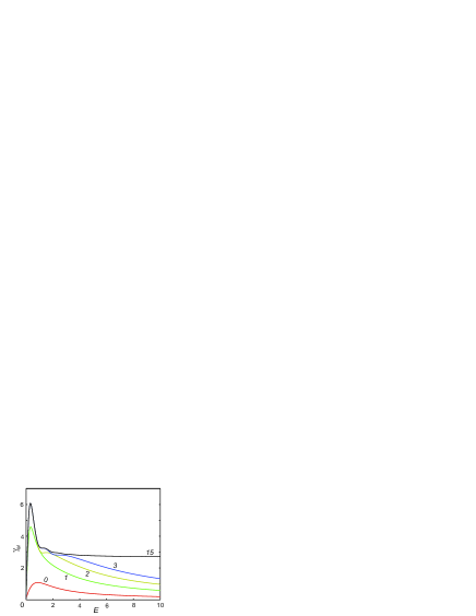
Figure 3: (Color online) The contribution of the partial sums $\gamma_{M}$ to the inverse momentum relaxation time. The italic numbers on the curves indicate the number $M$ where $M=15$ corresponds to the convergent result.

It’s behavior is qualitatively similar to the one for the total cross-section. For large energies it approaches the limiting value $\gamma=8/3$, which we obtain by calculating the integral (8) with the classical differential cross-section, confirming the known fact that the integral (8) is not sensitive to forward scattering. Thus this relaxation time isn’t affected by the above mentioned discrepancy between the quantum and classical result as it was with the total cross-section.

Note that there is an essential difference in the separate contributions to the total cross-section $\sigma$ and the inverse momentum relaxation time $\gamma$. The partial contributions to $\gamma$ do not exhibit any oscillating behavior that was inherent in the case of $\sigma$. This is expected from Eq. (39) where the difference of neighboring phases $(\delta_{m}-\delta_{m+1})$ doesn’t depend on energy in the asymptotic region.

And at last inserting the differential cross-section (35) into Eq. (9) we obtain the perpendicular (or Hall) component of the conductivity

$$\begin{split}\eta=&-\frac{2i}{\pi E}\sum_{m,m^{\prime}=-\infty}^{\infty}\left[\delta_{m^{\prime},m+1}-\delta_{m^{\prime},m-1}\right]\\ &\phantom{mmmmmm}\times e^{i(\delta_{m^{\prime}}-\delta_{m})}\sin\delta_{m}\sin\delta_{m^{\prime}}\\ =&\frac{4}{E}\sum_{m=-\infty}^{\infty}\sin\delta_{m}\sin\delta_{m+1}\sin\left(\delta_{m+1}-\delta_{m}\right).\end{split}$$ (42)

The result is shown in Fig. 4.

Figure 4: The Hall component of resistivity.

Naively we would expect that $\eta=0$ at zero magnetic field. To our surprise we find that $\eta<0$ and that it conserves it’s sign as a function of $E$. It means that the mass barrier acts similar as a magnetic field. In order to obtain the result for $K^{\prime}$ valley electrons we have to change $m\to-m$ and $m^{\prime}\to-m^{\prime}$ in the arguments of Kronecker symbols in the first line of Eq. (42). It is evident that due to this change the Hall component of the resistivity $\eta$ changes it’s sign. Thus, the electrons from different valleys are deflected to opposite sides of the sample. There is no net charge build up across the sample and thus no Hall voltage. But there is a separation of different $K$ and $K^{\prime}$ valley electrons across the sample and thus we can use this effect for valley filtering purposes.

VI Scattering on a penetrable circle

Now we turn to our last problem — scattering of Dirac electrons by a penetrable circle in order to demonstrate how possible quasi-bound states reveal themselves in the scattering cross-section. For this purpose we have to solve the Dirac equation for free electrons (25) in both $I$ and $III$ regions and to apply boundary conditions (19). These solutions are given by Eq. (26) for the inner region $I$, and by Eq. (28) for the outer region $III$. Moreover, the procedure of the exclusion of the incident exponent is the same as it was performed in Sec. V. Thus we can immediately write down Eqs. (34) for the components of the scattering amplitudes, and use the previous expressions for the scattering cross-section (35,37,41,42).

The single procedure that should be performed is to satisfy the boundary conditions (19) and calculate the phase shifts $\delta_{m}$. Inserting into Eq. (19) the solutions (26) and (28) we obtain the set of two equations:

$$CJ_{m+1}+SY_{m+1}-FJ_{m+1}$$ (43a)

$$=-P\left\{CJ_{m}+SY_{m}+FJ_{m}\right\},$$

$$CJ_{m}+SY_{m}-FJ_{m}$$ (43b)

$$=-P\left\{CJ_{m+1}+SY_{m+1}+FJ_{m+1}\right\},$$

where for the sake of shortness we denoted

$$C=w_{m}\cos\delta_{m},\quad S=w_{m}\sin\delta_{m},$$ (44)

and omitted the arguments $E$ of all Bessel functions.

Now excluding coefficient $F$ we obtain a single equation. It can be solved for the tangent of the phase shift, and using the expression for the Wronskian of the Bessel functions we arrive at

$$\tan\delta_{m}=-\frac{(J_{m+1}+J_{m})(J_{m}-J_{m+1})}{(Y_{m+1}+Y_{m})(J_{m}-J_{m+1})-1/pE},$$ (45)

where the symbol

$$p=\frac{\pi P}{(1-P)^{2}}$$ (46)

characterizes the impenetrability of the circle. The value $p=\infty$ corresponds to a completely impenetrable circle, i. e. the previously considered scattering on an impenetrable anti-dot, while the value $p=0$ corresponds to the case of complete penetration, or the absence of any scatterer.

The numerical results for the lowest contribution ($m=0$) to the total cross-section are shown in Fig. 5 for different $p$ values.

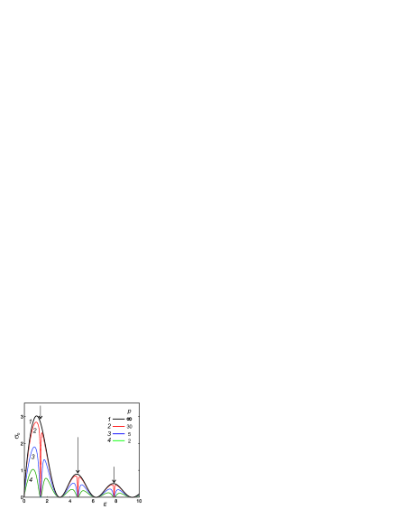
Figure 5: (Color online) The partial $\sigma_{0}$ contribution to the total cross-section for different values of the penetrable parameter $p$ of the circular scatterer. The curve marked by $p=\infty$ corresponds to the case of scattering by an impenetrable circle.

The vertical lines indicate the energies of the bound states of the dot obtained by solving Eq. (27) as described in Sec. IV. Although now the dot is penetrable and it has no bound states, the corresponding quasi-bound states reveal themselves as narrow gaps close to the maxima of the oscillating partial contribution. Note that this is a particular feature of Dirac electrons. While in the case of Schrödinger electrons the quasi-bound states appear as peaks in the cross-section (see Figs. 10 and 11 in Appendix A).

According to Eq. (45) it seems that there should be one more set of gaps in the partial cross-section, related to the equation

$$J_{m}(E)+J_{m+1}(E)=0.$$ (47)

But in this case, however, after neglecting the last term in the denominator of Eq. (45) it coincides with the phase (29) obtained for the scattering by the impenetrable circle, and in such a way it indicates that the above condition defines the flat minimum related to the diffraction pattern in the cross-section considered in Sec. V.

These gaps in the partial cross-section reveal themselves in the total cross-section as shown in Fig. 6.

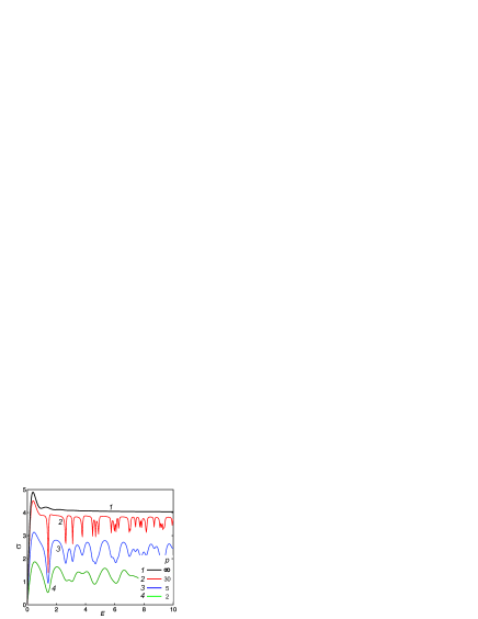
Figure 6: (Color online) The total cross-section $\sigma$ for a penetrable circular scatterer for different $p$ values. The curve marked by $p=\infty$ corresponds to the case of scattering on an impenetrable circle.

Because of the contribution of the other partial waves the gaps no longer reach zero as e. g. shown in the case of the partial cross-section $\sigma_{0}$. Notice that they become more pronounced and narrower when the parameter $p$ increases (when the circle becomes less penetrable).

In Fig. 7 the results for the inverse momentum relaxation time and in Fig. 8 those for the perpendicular component of the resistivity are presented.

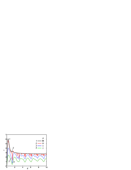
Figure 7: (Color online) The inverse momentum relaxation time calculated according Eq. (41) for a penetrable circular scatterer.

We see that although Eqs. (41) and (42) are more sophisticated functions of the phases

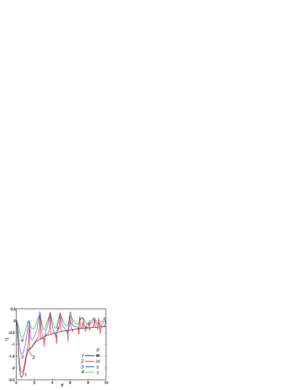
Figure 8: (Color online) The Hall component $\eta$ calculated according Eq. (42) for a penetrable circular scatterer.

$\delta_{m}$ and even two neighboring phases $\delta_{m}$ and $\delta_{m+1}$ are intermixed, nevertheless the resonant behavior, i. e. the negative peaks, is still clearly visible in the inverse momentum relaxation time. The behavior of peaks in the Hall component of the resistivity, however, is more complicated, and exhibits both sharp peaks and dips where now the sign of $\eta$ can change in small regions of energy.

VII Conclusions

We investigated the scattering of Dirac electrons by sharp circular mass barriers, where we studied both hard wall type anti-dot and circular penetrable scatterer. For this purpose the proper boundary conditions for Dirac equation were derived, and it was illustrated how it is possible to use formally $\delta$-type functions describing relativistic systems with high and sharp potentials.

The differential and total cross-section, the inverse momentum relaxation time and the perpendicular (Hall) component of resistivity were calculated. The obtained results were compared with analogous results for scattering of Schrödinger electrons by similar scatterers.

It was shown that the scattering of Dirac electrons even by azimuthal symmetric structures depends on the valley index: the $K$ valley electrons are preferentially deflected to one side (the Hall component of the resistivity isn’t zero) while the electrons of the other $K^{\prime}$ valley are deflected to the other side of the sample. This enables one to use this property for valley index filtering in transport experiments.

There is an essential difference in the energy dependence of the cross-section between Dirac and Schrödinger electrons. At small energies the cross-section for Dirac electrons tend to zero while those for Schrödinger electrons diverge logarithmically. This feature of Dirac electron is caused by the fact that zero energy for Dirac electron actually corresponds to the middle of the half-filled band, and not to the bottom of it as in the Schrödinger electron case.

We showed that in the case of Dirac electron scattering on a penetrable circle the quasi-bound states reveal themselves as sharp gaps in the total cross-section, the inverse momentum relaxation time and the Hall component of the resistivity as well. In the case of Schrödinger electrons those resonances show up as peaks in the cross-sections, and thus their appearance is qualitatively very different.

Appendix A Scattering of a Schrödinger electron by circular barriers

In this Appendix we study the scattering of Schrödinger electrons by sharp circular potentials shown in Fig. 1. This allows us to compare them with results for Dirac electrons considered in the present paper.

Here scattering is now described by the single component wave function $\Psi({\bf r})$ satisfying the stationary Schrödinger equation

$$(\nabla^{2}+k^{2})\Psi(\bi{r})=0,$$ (48)

where the symbol $k$ stands for the electron momentum related to it’s energy as $E=k^{2}/2$. Now we use dimensionless units defined as follows. The coordinates will be measured in the radius of the circular scatterer $R$, energy — in $\hbar^{2}/mR^{2}$ units, and the electron momentum — in $\hbar/R$ units.

In polar coordinates the wave function $\Psi({\bf r})$ is usually expanded into a Fourier series like $U({\bf r})$ component of Dirac function in Eq. (12) with radial components $\psi_{m}(r)$ satisfying the Bessel equation. That is why all mathematics is practically the same as used in previous sections with a single replacement of the Dirac electron energy $E$ by the momentum $k$ of the Schrödinger electron. Consequently, we obtain the same differential cross-section given by Eq. (35), and Eqs. (37) and (41) for the total cross-section and inverse momentum relaxation time.

Nevertheless, there is an essential difference between Dirac and Schrödinger electrons which is the different boundary conditions that will lead to different scattering phases.

Thus, in the case of scattering on a circular hard wall potential (see Fig. 1(a)) every radial component of the wave function has to satisfy the zero boundary condition

$$\psi_{m}(1)=0,$$ (49)

what leads to the following equation for the phase

$$\tan\delta_{m}=-\frac{J_{m}(ka)}{Y_{m}(ka)},$$ (50)

instead of Eq. (29) for the Dirac electron. The partial contributions and the total cross-section calculated by using the above phase equation are shown in Fig. 9.

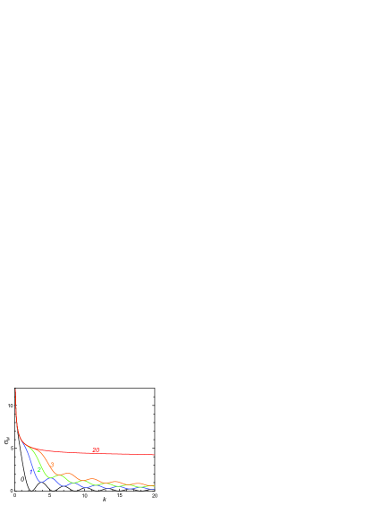
Figure 9: (Color online) The energy dependence of the partial sums $\sigma_{M}$ contributing to the total cross-section for Schrödinger electrons. The italic numbers on the curves indicate the number $M$.

In the case of an extremely narrow penetrable circle, i. e. a $\delta$-type potential, Eq. (48) has to be replaced by

$$\left\{\nabla^{2}+k^{2}-p\delta(r-1)\right\}\Psi(\bi{r})=0$$ (51)

what leads to the following boundary conditions for the radial wave function components on the circle:

$$\psi_{m}(1+0) = \psi_{m}(1-0),$$ (52a)

$$\psi^{\prime}_{m}(1+0)-\psi^{\prime}_{m}(1-0) = p\psi_{m}(1).$$ (52b)

This leads to the following scattering phase equation:

$$\tan\delta_{m}=-\frac{J_{m}(k)}{Y_{m}(k)-2/p\pi J_{m}(k)}.$$ (53)

From it we obtain the following partial contribution to the total cross-section:

$$\frac{4}{k}\sin^{2}\delta_{m}=\frac{4J_{m}^{2}(k)}{k\left\{J_{m}^{2}(k)+[Y_{m}(k)-2/p\pi J_{m}(k)]^{2}\right\}}.$$ (54)

The typical contribution(when $m=0$) is shown in Fig. 10 by red solid curve.

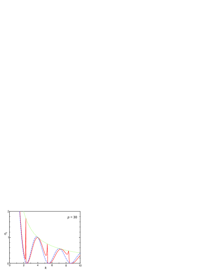
Figure 10: (Color online) The $m=0$ contribution to the total cross-section for Schrödinger electrons scattered on penetrable circular potentials, shown by red solid curve. Green dotted curve is the envelop function $4/k$, and the blue dashed curve is the result for scattering on impenetrable scatterers.

Narrow peaks appear close to the positions of the bound states of a dot that are defined by the equation $J_{m}(k)=0$. This can be also seen from Eq. (54) which formally is similar to a Lorentzian curve. The top of the peak is achieved when the second term in the denominator (the analog of detuning) in Eq. (54) is zero. In the case of small penetrability of the scatterer this can be realized if the large parameter $p\gg 1$ is compensated by a small $J_{m}(k)\ll 1$ value. But then the contribution becomes equal to $4/k$ what indicates that the maximum of all peaks reach the above envelope function shown by green dotted curve in Fig. 10. One more property of the partial contribution follows from the fact that it is rather close to the same contribution in the case of scattering by impenetrable scatterer shown by the blue dashed curve (Eq. (53) converts itself into Eq. (50) when $p=\infty$) what indicates that the peaks appear at the minima of that dashed curve.

These resonances show up also in the total cross-section as seen in Fig. 11.

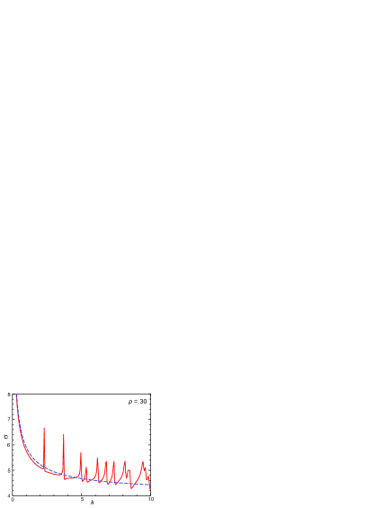
Figure 11: (Color online) The same as Fig. 10 but now for the total cross-section.

The comparison with the blue dashed curve calculated for $p=\infty$ indicates clearly that the quasi-bound states appear in the total cross-section as positive peaks.

References

- (1) D. K. Ferry and S. M. Goodnick, Transport in Nanostructures (Cambridge University Press, 2001).
- (2) T. Ando, A. B. Fowler and F. Stern, Rev. Mod. Phys. 54, 437 (1982).
- (3) K. S. Novoselov, A. K. Geim, S. V. Morozov, D. Jing, M. I. Katsnelson, I. V. Grigorieva, S. V. Dubonos, and A. A. Firsov, Nature (London) 438, 197 (2005).
- (4) Y. Zang, Y. W. Tan, H. L. Stormer, and P. Kim, Nature (London) 438, 201 (2005).
- (5) A.V. Rozhkov, G. Giavaras, Y.P. Bliokh, V. Freilikher, F. Nori, Phys. Reports 503, 77 (2011).
- (6) J. Moore, Nature (London) 464, 194 (2010).
- (7) M. Z. Hasan and C. L. Kane, Rev. Mod. Phys. 82, 3045 (2010).
- (8) G. W. Semenoff, Phys. Rev. Lett. 53, 2449 (1984).
- (9) P. R. Wallace, Phys. Rev. 71, 622 (1947).
- (10) I. Zutic, J. Fabian, and S. Das Sarma, Rev. Mod. Phys. 76, 323 (2004).
- (11) A. Rycerz, J. Tworzydlo, and C. W. J. Beenakker, Nature Phys. 3, 172 (2007).
- (12) D. Gunlycke and C. T. White, Phys. Rev. Lett. 106, 136806 (2011).
- (13) J. Lahiri, Y. Lin, P. Bozkurt, I. I. Oleynik, and M. Batzill, Nature Nanotech. 5, 326 (2010).
- (14) P. Y. Huang, C. S. Ruiz-Vargas, A. M. van der Zande, W. S. Whitney, M. P. Levendorf, J. W. Kevek, S. Garg, J. S. Alden, C. J. Hustedt, Y. Zhu, J. Park, P. L. McEuen, and D. A. Muller, Nature (London) 469, 389 (2011).
- (15) C. L. Roy, Phys. Rev. A 47, 3417 (1993).
- (16) J. J. Sakurai, Modern Quantum Mechanics, Addison-Wesley Publishing Company, Reading (1994).