Decoherence in an accelerated universe

Abstract

In this paper we study the decoherence processes of the semiclassical branches of an accelerated universe due to their interaction with a scalar field with given mass. We use a third quantization formalism to analyze the decoherence between two branches of a parent universe caused by their interaction with the vaccum fluctuations of the space-time, and with other parent unverses in a multiverse scenario.

I Introduction

Decoherence plays a fundamental role in quantum mechanics and cosmology. It effectively collapses the wave function from a superposition of states to the observed component Kiefer (2007). In particular, decoherence is responsible for the collapse of the wave function and becomes the ultimate reason for the appearance of a classical universe in quantum cosmology Kiefer (2007); Joos et al. (2003).

In a decoherence process we have first to identify the system under study and its environment, i.e. we have to distinguish relevant from irrelevant variables Kiefer (2007). This sort of choice is usually based on the particular features of the experiment, though it can become somehow arbitrary. Decoherence clearly depends on that choice and it is therefore related to the separability of the whole quantum system into the system under study and its environment. Thus, different subsystems can effectively be considered to be the environment of a quantum system.

Moreover, decoherence and dissipative processes between a system and its environment make the state of the system evolve to a state of higher entropy Kiefer (2007). In quantum cosmology, such a entropy increasing provides us with an arrow of time and it is thus the responsible for the irreversibility in the universe. Strictly speaking, time can only be considered when a decoherence process has taken place and the semiclassical branches of the universe have emerged.

The interaction between an homogeneous and isotropic universe and the density fluctuations and gravitational waves has been studied in Refs. Zeh (1986); Halliwell (1989); Kiefer (1992); Coleman (1988a, b); González-Díaz (1992a). In this case, the relevant variables are the scale factor and the homogeneous degrees of freedom of the scalar field. The non-observable degrees of freedom, which are traced out from the state of the universe, have however observable effects on the properties of the semiclassical branch of the universe.

Among these effects, it can be pointed out: i) the decoherence of different branches of the universe Halliwell (1989); Kiefer (1992), the shift of the coupling constants and the reduction of the value of the cosmological constant Coleman (1988a, b), and the modification of the coherence properties of the fields that propagate in the space-time Coleman (1988a); González-Díaz (1992a).

In this paper, we review the effects that decoherence processes can produce on the state of an homogeneous and isotropic branch of an accelerating universe. In Sec. II, we apply the formalism developed in Refs. Halliwell (1989); Kiefer (1992) to analyze the decoherence between the expanding and contracting branches of the universe due to the interaction with a scalar field, for quintessence-dominated, vacuum-dominated and phantom-dominated universes. The third quantization formalism is used in Sec. III to study the interaction between parent universes and between a parent universe and a plasma of baby universes which represent, in a first approximation, the quantum fluctuations of the space-time of the parent universe, following the parallel quantum optics developments. In Sec. IV, we shall draw some conclusions.

II Decoherence of the branches of an accelerating universe

In Refs. Halliwell (1989); Kiefer (1992, 2007), the inhomogeneous modes of a scalar field are taken as the irrelevant variables in order to obtain a reduced density matrix that represented the quantum state of the homogeneous universe. The inhomogeneous modes were coupled to the metric of a spatially closed space-time Halliwell and Hawking (1985), which is assumed to be in the semiclassical regime. The result is that the expanding and contracting branches of the universe are quickly decoupled for large values of the scale factor. Thus, the universe is either in an expanding or in a contracting state but not in a quantum superposition of both.

In a flat universe, the formalism used in Ref. Halliwell (1989) cannot be directly applied because the inhomogeneous modes of the massless scalar field are coupled to a zero curvature term of the metric Halliwell and Hawking (1985). However, we can consider a scalar field with a mass term which is minimally coupled to the curvature scalar. Except for this feature, in order to analyze the decoherence of the branches of the accelerated universe, we can follow the same procedure used in Ref. Halliwell (1989).

Let us consider therefore a flat homogeneous and isotropic universe which is dominated by a perfect fluid with equation of state $p=w\rho$, where $p$ and $\rho$ are the pressure and the energy density of the fluid, respectively, and $w$ is a constant parameter. Let us also consider a scalar field $\varphi$ with mass, $m$. The Wheeler-De Witt equation can be written, with the usual choice of the factor ordering Kiefer (2007), as

$$\left(a^{2}\partial^{2}_{aa}+a\partial_{a}+\frac{\Omega_{0}^{2}}{\hbar^{2}}a^{2q}-\partial^{2}_{\varphi\varphi}+\frac{m^{2}}{\hbar^{2}}a^{6}\varphi^{2}\right)\phi(a,\varphi)=0,$$ (1)

where $a$ is the scale factor, $\phi(a,\varphi)$ is the wave function of the universe, $\Omega_{0}^{2}$ is a constant which is proportional to the energy density of the universe at a given boundary hypersurface at $a_{0}$ González-Díaz and Robles-Pérez (2009), and, $q=\frac{3}{2}(1-w)$. The solutions of the gravitational part of Eq. (1) are given in terms of Bessel functions González-Díaz and Robles-Pérez (2008); Robles-Pérez and González-Díaz (2010),

$$\phi_{0}(a)\propto\mathcal{H}_{0}^{(1,2)}(\tilde{\Omega}_{0}a^{q}),$$ (2)

with $\tilde{\Omega}_{0}\equiv\frac{\Omega_{0}}{q\hbar}$, and, $\mathcal{H}_{n}^{(1)}$ and $\mathcal{H}_{n}^{(2)}$ are the Hankel function of first and second kind of order $n$. The boundary condition that has been used in Eq. (2) is the tunneling boundary condition Vilenkin (1986). In the asymptotic limit of large values of the scale factor Abramovitz and Stegun (1972), we have

$$\mathcal{H}_{0}^{(1,2)}(\tilde{\Omega}_{0}a^{q})\sim a^{-\frac{q}{2}}e^{\pm i(\tilde{\Omega}_{0}a^{q}-\frac{\pi}{4})},$$ (3)

where the $+$ and $-$ signs correspond to the Hankel function of the first and second kind, respectively. The solutions given by Eq. (3) describe the expanding and contracting branches of the semiclassical universe, as it can be checked by noting that the momentum operator is given by, $\hat{p}_{a}\phi(a)\equiv-i\hbar\partial_{a}\phi(a)\propto\pm\frac{\partial S_{0}}{\partial a}$, with $S_{0}=\tilde{\Omega}_{0}a^{q}$ the classical action, and the semiclassical momentum becomes, $p_{a}^{sc}=-a\dot{a}$. Then, $a\dot{a}\propto\mp\frac{\partial S_{0}}{\partial a}$. Thus, the Hankel function of the second kind corresponds to the expanding branch of the universe and the Hankel function of the first kind describes its contracting branch.

In the semiclassical regime, the wave function of the universe can be written as,

$$\phi(a,\varphi)=C(a)e^{\pm iS_{0}(a)}\chi(a,\varphi),$$ (4)

where $C(a)=a^{-\frac{q}{2}}$. The function $\chi(a,\varphi)$ satisfies the following Schrödinger equation Halliwell (1989); Kiefer (1992),

$$\frac{1}{2a^{3}}\left(-\frac{\partial^{2}}{\partial\varphi^{2}}+m^{2}a^{6}\right)\chi=i\frac{\partial\chi}{\partial t},$$ (5)

where the time variable $t$ is defined in terms of the scale factor through the classical equation, $a\dot{a}=\pm\Omega_{0}a^{q-1}$. Following the above references, we shall look for Gaussian solutions

$$\chi=A(a)e^{-B(a)\varphi^{2}}.$$ (6)

Inserting Eq. (6) into Eq. (5), we obtain a differential equation for the coefficients $A(a)$ and $B(a)$ that can be solved with the normalization condition, $\int d\varphi\chi\chi^{*}=1$. It is obtained

$$A = \pi^{-\frac{1}{4}}(B+B^{*})^{\frac{1}{4}}e^{i\alpha(t)},$$ (7)

$$B = \pm i\frac{\Omega_{0}}{2}a^{q+1}\frac{\dot{x}}{x},$$ (8)

where, $\dot{x}\equiv\frac{\partial x}{\partial a}$, and

$$a^{2}\ddot{x}+(1+q)a\dot{x}-\frac{m^{2}}{\Omega_{0}^{2}}a^{2(3-q)}x=0.$$ (9)

For a universe dominated by a cosmological constant ($w=-1$ and $q=3$), the solutions to Eq. (9) can be written as,

$$x=a^{-\frac{3}{2}}\left(c_{1}a^{k_{1}}+c_{2}a^{-k_{1}}\right),$$ (10)

with, $k_{1}=\frac{3}{2}\sqrt{1+\frac{4m^{2}}{9\Omega_{0}^{2}}}\approx\frac{3}{2}$. Choosing appropriate constants $c_{1}$ and $c_{2}$ to fulfill the condition, $B+B^{*}>0$, the value of the fucntion $B(a)$ can be approximated, in the semiclassical regime, as

$$B_{0}^{\pm}\approx\frac{\Omega_{0}}{2}\left(3\pm i\frac{m^{2}}{3\Omega_{0}^{2}}a^{3}\right),$$ (11)

where the positive and negative sign correspond to the solution of the function $\chi$ for the expanding and the contracting branches of the universe, respectively.

In the quintessence regime, for which $-\frac{1}{3}>w>-1$, the solutions of Eq. (9) can be written in terms of the modified Bessel functions of order $\nu$, $\mathcal{K}_{\nu}$ and $\mathcal{I}_{\nu}$. In the semiclassical regime, it reads

$$(B^{-}_{Q})^{*}=B^{+}_{Q}\approx\frac{\Omega_{0}}{2}\left(i\frac{m}{\Omega_{0}}+\pi(3+2|\beta|)a^{-\beta}e^{-2\lambda a^{\beta}}\right),$$ (12)

where, $q=\frac{3}{2}(1-w)\equiv 3-\beta$ (with, $1>\beta>0$), and $\lambda=\frac{m}{\Omega_{0}|\beta|}$.

In the phantom regime, for which $w<-1$ and $\beta<0$, the functions $B_{F}^{\pm}$ can be approximated in the semiclassical regime by,

$$(B^{-}_{F})^{*}=B^{+}_{F}\approx\frac{\Omega_{0}}{2}\left(-2iqa^{q}+c_{0}\right),$$ (13)

with $q=3+|\beta|$, and $c_{0}$ a positive constant.

Inserting these values of the functions $A(a)$ and $B(a)$ in Eq. (6), the reduced density matrix becomes

$$\rho_{r}(a,a^{\prime})=\int_{-\infty}^{\infty}d\varphi\chi^{*}(a,\varphi)\chi(a^{\prime},\varphi),$$ (14)

which is given, except for irrelevant phases, by Halliwell (1989)

$$\rho_{r}(a,a^{\prime})\propto\left[\frac{(B(a)+B^{*}(a))(B(a^{\prime})+B^{*}(a^{\prime}))}{(B^{*}(a)+B(a^{\prime}))^{2}}\right]^{\frac{1}{4}}.$$ (15)

For the case $w=-1$, Eq. (15) can be approximated in the semiclassical limit as,

$$\rho_{r}(a,a^{\prime})\approx\frac{1}{\sqrt{1\mp\frac{im^{2}}{18\Omega_{0}^{2}}(a^{3}-a^{\prime 3})}}.$$ (16)

The diagonal values of the reduced density matrix, for which $a\approx a^{\prime}$, become nearly unity. However, far from the diagonal elements, for which $a\gg a^{\prime}$, the reduced density matrix asymptotically vanishes, $|\rho_{r}|\sim a^{-\frac{3}{2}}$. That means that the decoherence process between the branches with different values of the scale factor is rather effective for large values of the scale factor, such as it should be expected.

In the quintessence regime,$-\frac{1}{3}\geq\omega\geq-1$ the decoherence process turns out to be even more effective. The reduced density matrix (15) can then be approximated as,

$$\rho_{r}(a,a^{\prime})\approx\sqrt{c}\left[\frac{(aa^{\prime})^{3-\beta}e^{-2\lambda(a^{\beta}-a^{\prime\beta})}}{\left(\mp i\frac{m}{2}(a^{3}-a^{\prime 3})+\frac{c}{2}(a^{3-\beta}e^{-2\lambda a^{\beta}}+a^{\prime 3-\beta}e^{-2\lambda a^{\prime\beta}})\right)^{2}}\right]^{\frac{1}{4}}.$$ (17)

For the diagonal values we have $\rho_{r}(a,a)\approx 1$, and for the off-diagonal values,

$$|\rho_{r}(a,a^{\prime})|\sim\left(\frac{a^{\prime}}{a}\right)^{\frac{q}{2}}a^{-\beta}e^{-\lambda a^{\beta}}\rightarrow 0\;\;(a\gg a^{\prime}>1).$$ (18)

Finally, for the phantom regime, $w<-1$ and $\beta<0$. For large values of the scale factor in that regime, but still before reaching the achronal region around the big rip singularity, where the semiclassical approximation is no longer valid Dabrowski et al. (2006),

$$\rho_{r}(a,a^{\prime})\approx\frac{1}{\sqrt{1\pm i\frac{q}{c_{0}}(a^{q}-a^{\prime q})}},$$ (19)

and, $|\rho_{r}|\sim a^{-\frac{q}{2}}$, for $a\gg a^{\prime}$. When the universe approaches the big rip singularity, the state of the universe is given by a quantum superposition of states Dabrowski et al. (2006), concordant with the expected quantum nature of the universe in such a region Dabrowski et al. (2006); Nojiri and Odintsov (2004).

It can be concluded that, both in a contracting and an expanding branch of an accelerated universe, the decoherence process between the scale factor and a scalar field is effective enough to remove the quantum interference between the different semiclassical branches that correspond to different values of the scale factor.

The same decoherence process turns out to be also effective to eliminate the interference between the contracting and expanding branches. If the state of the universe is given by a quantum superposition of the states that correspond to those branches, i.e.

$$\phi(a)\approx C(a)e^{-iS_{c}(a)}\chi^{+}(a,\varphi)+C^{*}(a)e^{iS_{c}(a)}\chi^{-}(a,\varphi),$$ (20)

with, $\chi^{+}=(\chi^{-})^{*}$, then, the reduced density matrix will show four terms Halliwell (1989): the terms $\rho_{11}$ and $\rho_{22}$, which describe the quantum state of the expanding and contracting branches, respectively, are given by the expressions given above (Eqs. (16, 17,19)). The crossed terms, which correspond to the interference between the branches, are given by

$$(\rho_{21})^{*}=\rho_{12}=\int_{-\infty}^{\infty}d\varphi\chi^{+}(a,\varphi)(\chi^{-}(a^{\prime},\varphi))^{*}.$$ (21)

They turn out to be Halliwell (1989),

$$\rho_{12}(a,a^{\prime})\propto\left[\frac{(B^{+}(a)+\bar{B}^{+}(a))(B^{-}(a^{\prime})+\bar{B}^{-}(a^{\prime}))}{(B^{+}(a)+\bar{B}^{-}(a^{\prime}))^{2}}\right]^{\frac{1}{4}},$$ (22)

where, $\bar{B}\equiv B^{*}$. In that case, even for similar values of the scales factors, $a\approx a^{\prime}$, the elements of the reduced density matrix, $\rho_{12}$ and $\rho_{21}$, asymptotically vanish when the scale factor grows along the semiclassical regime. For instance, for a phantom dominated universe, $\rho_{12}$ turns out to be

$$\rho_{12}\approx\frac{1}{\sqrt{1-i\frac{q}{c_{0}}(a^{q}+a^{\prime q})}},$$ (23)

and the diagonal values,

$$|\rho_{12}(a,a)|\approx a^{-\frac{q}{2}}.$$ (24)

It means that the expanding and contracting branches of a phantom universe, which correspond to the regions far before and after the big rip singularity, decouple from each other in the semiclassical regime.

Therefore, the decoherence process between the scale factor and a scalar field with mass is seen to be effective enough to remove the interference terms between the different semiclassical branches of an accelerated universe. It eliminates both the interference terms between the expanding and contracting branches, and those between different branches that correspond to different values of the scale factor in the same expanding or contracting region of the universe.

In the case of a universe dominated by phantom energy, the big rip singularity makes it impossible a semiclassical description of the universe in the neighborhood of the singularity. There, the state of the universe is given by a quantum superposition of states Dabrowski et al. (2006) and the quantum effects are predominant Nojiri and Odintsov (2004). Moreover, the evolution becomes non-unitary in the achronal region around the big rip because of the presence of wormholes whose creation is induced by the exotic character of the phantom energy Sushkov (2005); Lobo (2005); González-Díaz (2003). Therefore, a generalized quantum theory González-Díaz and Robles-Pérez (2009) has to be used to give a proper quantum description of the whole phantom universe.

III Decoherence in a third quantization scheme

III.1 Parent and baby universes

In a third quantization formalism Strominger (1990), the field to be quantized is the wave function of the universe. Then, the state of the multiverse can be studied as a quantum field theory in the superspace.

Let us consider the Wheeler-De Witt equation (1) with no scalar field and without any factor ordering terms, i.e.

$$\ddot{\phi}+\Omega^{2}(a)\phi=0,$$ (25)

where the overhead dot means derivative with respect to the scale factor. Eq. (25) can be seen as the classical equation of motion for a harmonic oscillator with a time dependent frequency, with the scale factor playing the role of the time variable. The wave function of the multiverse satisfies then the Schrödinger equation,

$$\mathbf{\mathrm{H}}|\Psi\rangle=i\hbar\frac{\partial}{\partial a}|\Psi\rangle,$$ (26)

with,

$$\mathbf{\mathrm{H}}=\frac{1}{2}\hat{P}_{\phi}^{2}+\frac{\Omega^{2}(a)}{2}\hat{\phi}^{2}.$$ (27)

$\hat{\phi}$ and $\hat{P}_{\phi}$ respectively are the operators of the wave function of a single universe and its conjugate momentum, in the Schrödinger picture. Going into Heisenberg picture, these operators can be written as

$$\hat{\phi}(a) = A(a,a_{0})\hat{\phi}+B(a,a_{0})\hat{P}_{\phi},$$ (28)

$$\hat{P}_{\phi}(a) = \dot{A}(a,a_{0})\hat{\phi}+\dot{B}(a,a_{0})\hat{P}_{\phi},$$ (29)

where the functions $A(a,a_{0})$ and $B(a,a_{0})$ satisfy Eq. (25) with the initial conditions, $A(a_{0},a_{0})=\dot{B}(a_{0},a_{0})=1$ and $\dot{A}(a_{0},a_{0})=B(a_{0},a_{0})=0$. The boundary condition that we impose to the quantum state of the multiverse is that the number of universes in the multiverse is constant along the evolution of the scale factor within a single universe. Then, the state of the multiverse is given in terms of the Lewis states Lewis and Riesenfeld (1969); Robles-Pérez and González-Díaz (2010), which are defined by the following creation and annihilation operators for universes,

$$b(a) \equiv \sqrt{\frac{1}{2\hbar}}\left(\frac{\hat{\phi}}{R}+i(R\hat{P}_{\phi}-\dot{R}\hat{\phi})\right),$$ (30)

$$b^{\dagger}(a) \equiv \sqrt{\frac{1}{2\hbar}}\left(\frac{\hat{\phi}}{R}-i(R\hat{P}_{\phi}-\dot{R}\hat{\phi})\right),$$ (31)

where $R\equiv R(a)$ is a function that satisfies the auxiliary equation, $\ddot{R}+\Omega^{2}(a)R-\frac{1}{R^{3}}=0$. In terms of the operators (30-31), the third quantized Hamiltonian (27) turns out to be

$$\mathbf{\mathrm{H}}=\hbar\left[\beta_{-}b^{2}+\beta_{+}{b^{\dagger}}^{2}+\beta_{0}\left(b^{\dagger}b+\frac{1}{2}\right)\right],$$ (32)

where Robles-Pérez and González-Díaz (2010),

$$\beta_{+}^{*}=\beta_{-} = \frac{1}{4}\left\{\left(\dot{R}-\frac{i}{R}\right)^{2}+\Omega^{2}R^{2}\right\},$$ (33)

$$\beta_{0} = \frac{1}{2}\left(\dot{R}^{2}+\frac{1}{R^{2}}+\Omega^{2}R^{2}\right).$$ (34)

We can consider large universes with a characteristic length of order of the Hubble length of our universe. They will be called parent universes Strominger (1990). For large values of the scale factor, the non-diagonal terms in the Hamiltonian (32) vanish and the values of the coefficient $\beta_{0}$ asymptotically coincide with that of the proper frequency of the Hamiltonian Robles-Pérez and González-Díaz (2010). Then, the quantum correlations between the number states disappear and the quantum transitions between different number of universes are therefore forbidden for parent universes. Let us also notice that in that limit the adiabatic approximation is satisfied, $\frac{\dot{\Omega}}{\Omega}\ll\Omega$, and no creation of further universes can occur along the evolution of a parent universe.

Let us consider next the quantum fluctuations of the space-time of a parent universe, whose contribution to the wave function of the universe becomes important at the Planck scale Wheeler (1957). Some of these fluctuations can be viewed as tiny regions of the space-time that branch off from the parent universe and rejoin the large regions thereafter; thus, they can be then interpreted as virtual baby universes Strominger (1990). In that case Robles-Pérez and González-Díaz (2010), $\beta_{+}^{*}=\beta_{-}\rightarrow-\frac{\omega_{0}}{4}$ and $\beta_{0}\rightarrow\frac{\omega_{0}}{2}$, in Eq. (32), where $\omega_{0}$ is a constant that depends on the properties of the baby universe. The state of the gravitational vacuum is then represented by a squeezed state, with a particle creation of baby universes or fluctuations occuring along the expansion of the parent universe Grishchuk and Sidorov (1990).

Thus, parent and baby universes, which will be considered the subsequent sections, can be described in the context of a third quantization formalism as the states of a harmonic oscillator. The advantage of such a formalism becomes then clear: we can apply the well-studied machinery of harmonic oscillators and quantum field theory for the description of a parent universe or a plasma of baby universes. For instance, the propagator for the quantum state of a parent universe can be calculated from the propagator for the harmonic oscillator with time dependent frequency Khandekar and Lawande (1986) (see also Refs. Mukhanov and Winitzki (2007); Vergel and Villaseñor (2009)),

$$K(\Phi_{f},a;\Phi_{i},a_{0}) = \left[\frac{1}{2\pi i\hbar R(a)R(a_{0})\sin\alpha(a,a_{0})}\right]^{\frac{1}{2}}\exp\left[\frac{i}{2\hbar}\left\{\frac{\dot{R}(a)}{R(a)}\Phi_{f}^{2}-\frac{\dot{R}(a_{0})}{R(a_{0})}\Phi_{i}^{2}\right\}\right]$$ (36)

$$\exp\left[\frac{1}{2\hbar\sin\alpha(a,a_{0})}\left\{\left(\frac{1}{R^{2}(a)}\Phi_{f}^{2}+\frac{1}{R^{2}(a_{0})}\Phi_{i}^{2}\right)\cos\alpha(a,a_{0})-\frac{2}{R(a)R(a_{0})}\Phi_{i}\Phi_{f}\right\}\right],$$

where, $\Phi_{f}$ and $\Phi_{i}$, are the wave functions of the parent universe evaluated at two hypersurfaces given by the values of the scale factor $a$ and $a_{0}$, respectively, and $\alpha(a,a_{0})$ is defined as Lewis and Riesenfeld (1969); Robles-Pérez and González-Díaz (2010)

$$\alpha(a,a_{0})=\int_{a_{0}}^{a}\frac{da^{\prime}}{R^{2}(a^{\prime})}.$$

Another example is the density matrix that describes a heat bath of baby universes at temperature $T$. It can be written as the density matrix of a canonical ensemble of harmonic oscillators (see, for instance, Ref. Joos et al. (2003)),

$$\rho_{B}(\phi_{f},\phi_{i})=\prod_{n}\frac{\omega_{n}}{2\pi\sinh(\omega_{n}/kT)}\;\exp\left(-\frac{\omega_{n}}{2\sinh(\omega_{n}/kT)}[(\phi_{f,n}^{2}+\phi_{i,n}^{2})\cosh(\omega_{n}/kT)-2\phi_{f,n}\phi_{i,n}]\right),$$ (37)

where, $\phi_{f,n}$ and $\phi_{i,n}$, are the wave functions of the baby universes, which are represented by harmonic oscillators with frequency $\omega_{n}$, and the index $n$ labels the species of baby universes considered in the space-time foam.

III.2 Parent-baby interaction

Let us now pose the interaction scheme between a parent universe and its environment. First, we shall study the interaction between a parent universe and the quantum fluctuations of its space-time, being these represented by a plasma of baby universes. The gravitational vacuum will be considered in two different states: i) the state of a heat bath with temperature $T$, and ii) a squeezed vacuum state. Then, it will be analyzed the interaction of a parent universe with the rest of parent universes in the context of a multiverse.

The interaction between a parent universe and the quantum fluctuations of its space-time can be represented, in a first approximation, by a total Hamiltonian given by

$$H=H_{P}+H_{\varepsilon}+H_{int},$$ (38)

where $H_{P}$ is the Hamiltonian of the parent universe, $H_{\varepsilon}$ is the Hamiltonian of the plasma of baby universes, and $H_{int}$ is the interaction Hamiltonian. The former Hamiltonian is represented by a harmonic oscillator with a frequency that depends on the scale factor,

$$H_{P}=\frac{1}{2}P_{\Phi}^{2}+\frac{\Omega^{2}(a)}{2}\Phi^{2},$$ (39)

with, $q=\frac{3}{2}(1-w)$, and $\Omega(a)=\frac{\Omega_{0}}{q}a^{q-1}$, where $\Omega_{0}^{2}$ is proportional to the current energy density of our universe.

For the case of baby universes, the frequency of the harmonic oscillator can effectively be considered a constant determined by the energy and the characteristic length of the baby universe, which can go from the Planck length to the scale of laboratory physics in the dilute-gas approximation Farhi and Guth (1987); Kiefer (2007); Coleman (1988a, b). It is therefore very small compared with the large value of the length of the parent universe, which is of order of the Hubble length of our universe. Thus, the plasma of baby universes is represented in our model by a set of harmonic oscillators with constant frequency $\omega_{i}$, where the index $i$ labels the different species of baby universes, i.e.

$$H_{\varepsilon}=\sum_{i=1}^{N}\frac{1}{2}p_{\phi_{i}}^{2}+\frac{\omega_{i}^{2}}{2}\phi_{i}^{2},$$ (40)

The interaction Hamiltonian, $H_{int}$ in Eq. (38), can be written as

$$H_{int}=\sum_{i}\lambda_{i}\Phi_{P}\otimes f(\phi_{i}),$$ (41)

where $\lambda_{i}$ is an effective coupling constant between the parent universe and the baby universe $i$, which is assumed to be small so that the Born-Markov approximation can be assumed to hold in the interaction scheme. The form of $f(\phi_{i})$ depends on the kind of interaction which is considered to take place between the parent and the baby universes. For instance, in the case considered by Coleman Coleman (1988a, b) and others Giddings and Strominger (1988), in which simply-connected wormholes are considered and thus single baby universes are nucleated, $f(\phi_{i})\equiv\phi_{i}$. In the case considered by González-Díaz González-Díaz (1992b, a), where doubled-connected wormholes are created and therefore the baby universes are nucleated in pairs, $f(\phi_{i})\equiv\phi_{i}^{2}$. We shall consider these two cases in the analysis to follow. In general, $f(\phi_{i})$ can be a complicated function and these two extreme cases can be considered as the first terms of its series development.

As a result of the interaction between the parent universe and the plasma of baby universes, the properties of the parent universe are modified so that its evolution effectively becomes non-unitary. The master equation for the reduced density matrix of the parent universe, when the degrees of freedom of the baby universes are traced out, can be written as Schlosshauer (2007); Joos et al. (2003)

$$\partial_{a}\rho_{P}=-i[\tilde{H}_{P},\rho_{P}]-i\gamma[\Phi,\{P_{\Phi},\rho_{P}\}]-D[\Phi,[\Phi,\rho_{P}]]-f[\Phi,[P_{\Phi},\rho_{P}]].$$ (42)

The unitary part of the effective evolution of the parent universe, given by the first term in Eq. (42), corresponds to the evolution of a new harmonic oscillator, $\tilde{H}_{P}\equiv H_{P}+\frac{\tilde{\Omega}^{2}}{2}\Phi^{2}$, with a frequency which is shifted with respect to the initial value $\Omega(a)$. The corresponding Lamb shift is given by

$$\tilde{\Omega}^{2}(a)=-2\int_{a_{0}}^{a}da^{\prime}\,\eta(a,a^{\prime})A(a,a^{\prime}),$$ (43)

where $\eta(a,a^{\prime})$ is the imaginary part of the correlation function,

$$\langle\phi^{k}(a)\phi^{k}(a^{\prime})\rangle_{b}=\nu(a,a^{\prime})-i\eta(a,a^{\prime}),$$ (44)

with, $k=1$ and $k=2$, for linear and quadratic interactions, respectively, and $A(a,a_{0})$ is a solution of the Weeler-De Witt equation (25) (see, Eqs. (28-29)). The shift for the frequency of the harmonic oscillator that represents the state of the parent universe corresponds to a shift of its energy density. Therefore, the Lamb shift given by Eq. (43) can be viewed to be equivalent to the mechanism proposed by Coleman to set zero the most probable value of the cosmological constant into zero. It is currently known that the value of the cosmological constant is not zero but very small, in fact of the order of the current critical density.

Three terms can be distinguished in the non-unitary part of the master equation (42). The dissipation coefficient Schlosshauer (2007), $\gamma(a)$, is given by

$$\gamma(a)=\int_{a_{0}}^{a}da^{\prime}\,\eta(a,a^{\prime})B(a,a^{\prime}),$$ (45)

where $B(a,a_{0})$ is defined by Eqs. (28-29). In quantum mechanics, $\gamma$ is related to the momentum damping and to the velocity of the wave packet. However, the wave function of the universe is not defined upon the space-time but in the superspace so that the interpretation of $\gamma$ does not become so clear for the state of the multiverse.

The normal-diffusion coefficient Schlosshauer (2007), $D(a)$ in Eq. (42), is given by

$$D(a)=\int_{a_{0}}^{a}da^{\prime}\,\nu(a,a^{\prime})A(a,a^{\prime}),$$ (46)

where $\nu(a,a^{\prime})$ is the real part of the kernel (44). In quantum mechanics, $D$ gives a measure of the decoherence length of a Gaussian wave packet Schlosshauer (2007). In the case of the universe, this coefficient provides us therefore with a measure of the effectiveness of the decoherence process of two different branches of the universe, $\Phi$ and $\Phi^{\prime}$, caused by the interaction with the quantum fluctuations of the gravitational vacuum. Finally, the anomalous-diffusion coefficient Schlosshauer (2007) in Eq. (42) is given by,

$$f(a)=-\int_{a_{0}}^{a}da^{\prime}\,\nu(a,a^{\prime})B(a,a^{\prime}).$$ (47)

Let us now derive the results of in the third quantization formalism for linear and quadratic interactions. Two states are considered for the gravitational vacuum: i) a thermal state and, ii) a squeezed vacuum state.

III.2.1 Case 1: linear interaction

The wave functions that represent the baby universes are given by the solutions corresponding to the harmonic oscillator with constant frequency. These can be written, in terms of the creation and annihilation operators of baby universes, $b_{i}^{\dagger}$ and $b_{i}$, as

$$\phi_{i}(a)=\sqrt{\frac{1}{2\omega_{i}}}\left(e^{-i\omega_{i}(a-a_{0})}b_{i}+e^{i\omega_{i}(a-a_{0})}b_{i}^{\dagger}\right),$$ (48)

where $a$ is the scale factor of the parent universe, and $b_{i}^{\dagger}$ and $b_{i}$, are the creation and annihilation of baby universes evaluated at the hypersurface given by the value $a_{0}$. Then, for the case of linear interaction, $k=1$ in the correlation function (44). In the case of a thermal bath of baby universes, $\langle b_{i}^{2}\rangle_{b}=\langle(b_{i}^{\dagger})^{2}\rangle_{b}=0$ and $\langle b_{i}^{\dagger}b_{i}\rangle_{b}=N_{i}(T)=\langle b_{i}b_{i}^{\dagger}\rangle_{b}-1$, with

$$N_{i}(T)=\frac{1}{e^{\frac{\omega_{i}}{T}}-1},$$ (49)

where $T$ is the temperature of the space-time foam Garay (1998), in units $\frac{k_{B}}{\hbar}=1$. The noise kernel Schlosshauer (2007), $\nu(a,a^{\prime})$, and the dissipation kernel Schlosshauer (2007), $\eta(a,a^{\prime})$, in Eq. (44), can be written then as

$$\nu(a-a^{\prime}) = \sum_{i}\frac{\lambda_{i}^{2}}{2\omega_{i}}(2N_{i}+1)\cos\omega_{i}(a-a^{\prime}),$$ (50)

$$= \int_{0}^{\infty}d\omega J(\omega)\coth\left(\frac{\omega}{2T}\right)\cos\omega(a-a^{\prime})$$

$$\eta(a-a^{\prime}) = \sum_{i}\frac{\lambda_{i}^{2}}{2\omega_{i}}\sin\omega_{i}(a-a^{\prime}),$$ (51)

$$= \int_{0}^{\infty}d\omega J(\omega)\sin\omega(a-a^{\prime}),$$

where, $J(\omega)\equiv\sum_{i}\frac{\lambda_{i}^{2}}{2\omega_{i}}\delta(\omega-\omega_{i})$, is the spectral density of baby universes in the space-time foam. It encapsulates the physical properties of the plasma of baby universes. For the quantum fluctuations of the gravitational vacuum, it is expected that the presence of baby universes in the space-time foam be exponentially suppressed for large values of the energy of the baby universe. Therefore, we assume the following spectral density for the bath of baby universes, $J(\omega)=J_{0}^{2}\omega^{3}e^{-\frac{\omega}{\Lambda}}$, where $J_{0}$ and $\Lambda$ are two constants, the latter representing the cut-off for the energy of the vacuum fluctuations, and the factor $\omega^{3}$ has been introduced to make the value of $J(\omega)$ sufficiently convergent at $\omega\rightarrow 0$.

The functions $A(a,a_{0})$ and $B(a,a_{0})$ in Eqs. (28-29) and Eqs. (43-47) can be expressed in terms of Bessel functions. For large values of the scale factor, which correspond to the description of parent universes, they can be approximated as

$$A(a,a^{\prime}) = \left(\frac{a^{\prime}}{a}\right)^{\frac{q-1}{2}}\cos\left(\frac{\Omega_{0}}{q}(a^{q}-a^{\prime q})\right),$$ (52)

$$B(a,a^{\prime}) = (aa^{\prime})^{\frac{1-q}{2}}\frac{1}{\Omega_{0}}\sin\left(\frac{\Omega_{0}}{q}(a^{q}-a^{\prime q})\right).$$ (53)

where $q=\frac{3}{2}(1-w)$. For, $q=1$ ($w=\frac{1}{3}$), these equations are exact and correspond to the solutions of a harmonic oscillator with constant frequency, $\Omega_{0}$. If we consider small changes in the scale factor of the parent universe, $a-a_{0}\ll 1$ and $a-a^{\prime}\ll 1$, then,

$$\tilde{\Omega}^{2}(a) \approx -\frac{2c_{1}a^{2}}{n_{1}n_{2}}\left(1-n_{2}\left(\frac{a_{0}}{a}\right)^{n_{1}}+n_{1}\left(\frac{a_{0}}{a}\right)^{n_{2}}\right)$$ (54)

$$D(a) \approx \frac{c_{2}a}{n_{1}}\left(1-\left(\frac{a_{0}}{a}\right)^{n_{1}}\right),$$ (55)

with, $n_{1}=\frac{q+1}{2}$, $n_{2}=\frac{q+3}{2}$, and

$$c_{1} = \int_{0}^{\infty}d\omega\,\omega J(\omega)\approx 24J_{0}^{2}\Lambda^{5},$$ (56)

$$c_{2} = \int_{0}^{\infty}d\omega J(\omega)\coth\left(\frac{\omega}{2T}\right)\approx 4J_{0}^{2}\Lambda^{3}T,$$ (57)

where the limit $\frac{\omega}{T}\ll 1$, has been taken in the latter equation.

On the other hand, if we describe the plasma of baby universes by a squeezed state, which can be considered a more realistic case Grishchuk and Sidorov (1990); Kiefer (2007), then

$$\langle b_{i}^{\dagger}b_{i}\rangle = \sinh^{2}r_{i}\equiv\tilde{N}_{i},$$ (58)

$$\langle b_{i}b_{i}^{\dagger}\rangle = \cosh^{2}r_{i}\equiv\tilde{N}_{i}+1,$$ (59)

$$\langle b_{i}^{2}\rangle = -\frac{1}{2}e^{i\theta_{i}}\sinh 2r_{i},$$ (60)

$$\langle(b_{i}^{\dagger})^{2}\rangle = -\frac{1}{2}e^{-i\theta_{i}}\sinh 2r_{i},$$ (61)

where $r_{i}$ and $\theta_{i}$ are the squeezing parameters. The two first terms are equivalent to the case of a thermal bath of baby universes with an effective number of quanta given by, $\tilde{N}_{i}\equiv\sinh^{2}r_{i}$. Thus, the dissipation kernel, $\eta(a,a^{\prime})$, turns out to be the same as in the thermal case, as it is also given by Eq. (51). Then, the Lamb shift $\tilde{\Omega}(a)$ is that given by Eq. (54). However, the squeezed vacuum introduces new terms in the noise kernel, $\nu(a,a^{\prime})$. This is given in the case of the squeezed vacuum by

$$\nu_{s}(a-a^{\prime}) = \sum_{i}\frac{\hbar\lambda_{i}^{2}}{2\omega_{i}}\{(2\tilde{N}_{i}+1)\cos\omega_{i}(a-a^{\prime})$$ (62)

$$- \sinh 2r_{i}\cos(\omega_{i}(a+a^{\prime}-2a_{0})-\theta_{i})\}.$$

Then, the decoherence factor, $D(a)$, turns out to be given by Eq. (55), with

$$c_{2}^{s}=\int_{0}^{\infty}d\omega J(\omega)\left(\cosh 2r-\sinh 2r\cos\theta\right).$$ (63)

A similar expression is obtained in Ref. Joos et al. (2003), p. 217 (see, also, Ref. Kiefer and Polarski (1998)). There, a decoherence timescale is given by, $t_{D}^{-1}=\sqrt{c_{2}^{s}}$. In the limit of large squeezing Joos et al. (2003), $\theta\rightarrow 0$ and $r\rightarrow-\infty$, and we can estimate a decoherence scale for two different branches of the parent universe given by, $a_{D}\approx\frac{1}{J_{0}\Lambda^{2}e^{|r|}}$.

In both, a vacuum in a thermal and in a squeezed state, the effect of decoherence due to the interaction of the parent universe with the quantum fluctuations of the space-time is similar if effectively we assume that, $T\sim\Lambda N$ in the thermal bath, and that, $e^{2|r|}\sim N$, in the squeezed vacuum; that is, for a large number of fluctuations of the space-time.

On the other hand, the timescale for the decoherence of a wave packet is differently analyzed in Ref. Schlosshauer (2007). There, the decoherence factor $D$ measures the decoherence of a Gaussian wave packet at spatial positions $x$ and $x^{\prime}$, with a decoherence time given by Schlosshauer (2007), $\tau_{D}=\frac{1}{D(x-x^{\prime})^{2}}$. In the case of the universe, $\Phi$ and $\Phi^{\prime}$ represent different branches of the parent universe, and therefore, a decoherence scale of order $a_{D}\sim\frac{1}{c_{2}(\Phi-\Phi^{\prime})^{2}}$ can be assumed, with $c_{2}$ as given by Eq. (57) or Eq. (63) for the case of a thermal bath or a squeezed vacuum, respectively.

In any case, it can be concluded that the scale at which quantum interference between different branches of a parent universe becomes important is very small, presumably of order the Planck length.

III.2.2 Case 2: quadratic interaction

In the case of a quadratic interaction between the parent universe and the baby universes, $k=2$ in the correlation function given by Eq. (44). The formalism applies in the same way as in all the previous cases and the quadratic interaction only changes the functional form of the dissipation and noise kernels, $\eta(a,a^{\prime})$ and $\nu(a,a^{\prime})$, respectively. For a vacuum in a thermal state and $a-a_{0}\ll 1$, they are given by

$$\eta(a,a^{\prime}) = 4\int_{0}^{\infty}d\omega J(\omega)N(a-a^{\prime}),$$ (64)

$$\nu(a,a^{\prime}) = 2\int_{0}^{\infty}d\omega\frac{J(\omega)}{\omega}N^{2},$$ (65)

where, $N\equiv N(\omega)$, is defined in Eq. (49). Then, the Lamb shift, $\tilde{\Omega}(a)$, and the decoherence factor, $D(a)$, are those given by Eqs. (54) and (55), respectively, with new coefficients $d_{1}$ and $d_{2}$ instead of $c_{1}$ and $c_{2}$, given by

$$d_{1} = 8T\int_{0}^{\infty}d\omega\;\frac{J(\omega)}{\omega}\approx 16J_{0}^{2}\Lambda^{3}T,$$ (66)

$$d_{2} = 8T^{2}\int_{0}^{\infty}d\omega\frac{J(\omega)}{\omega^{3}}\approx 8J_{0}^{2}\Lambda T^{2}.$$ (67)

For a squeezed vacuum state, the leading terms of the dissipation and noise kernels turn out to be

$$\eta(a,a^{\prime}) \approx \int_{0}^{\infty}d\omega J(\omega)e^{2|r|}(a-a^{\prime}),$$ (68)

$$\nu(a,a^{\prime}) \approx \int_{0}^{\infty}\frac{J(\omega)}{2\omega}e^{4|r|},$$ (69)

and then

$$d_{1}^{s} \approx 6J_{0}^{2}\Lambda^{4}e^{2|r|},$$ (70)

$$d_{2}^{s} \approx J_{0}^{2}\Lambda^{3}e^{4|r|}.$$ (71)

For the quadratic interaction, therefore, the coefficient $d_{1}$ that determines the Lamb shift depends on the temperature, for a thermal vacuum, and on the squeezing parameter $r$, for a squeezed vacuum state. It depends thus on the strength of the fluctuations of the space-time of the parent universe, which is assumed to be large. The coefficient of the decoherence factor, $d_{2}$, depends on $\tilde{N}_{i}^{2}$ in the quadratic interaction. However, this kind of interaction is of order $\hbar^{2}$ instead of $\hbar$ for linear interaction, and therefore the contribution of the quadratic interaction is subdominant in the semiclassical regime of the quantum state of the universe.

III.3 Parent-parent interaction

We can also consider the interaction between a parent universe and the rest of universes of a multiverse made up of parent universes. In that case, the squeezing effect of the state of the multiverse asymptotically disappears Robles-Pérez and González-Díaz (2010), i.e. $r\rightarrow 0$ as $a\rightarrow\infty$. It seems then most appropriate considering a thermal state of $N$ parent universes, with $N^{-1}=e^{\frac{\omega}{T}}-1$, where $T$ is a temperature analog in the multiverse. It includes the special case for which $N=0$ ($T=0$) that represents the interaction of a parent universe with the fluctuations of its ground state.

For parent universes, the coefficients of their wave functions can be approximated by Eqs. (52-53), and then

$$\tilde{\Omega}^{2}(a) \approx -\frac{2}{a^{q-1}}\int_{a_{0}}^{a}\int_{0}^{\infty}d\Omega^{\prime}J(\Omega^{\prime})\sin\frac{\Omega^{\prime}}{q}(a^{q}-a^{\prime q})\cos\frac{\Omega_{0}}{q}(a^{q}-a^{\prime q}),$$ (72)

$$D(a) \approx \frac{1}{a^{q-1}}\int_{a_{0}}^{a}\int_{0}^{\infty}d\Omega^{\prime}J(\Omega^{\prime})(2N+1)a^{\prime q-1}\cos\frac{\Omega^{\prime}}{q}(a^{q}-a^{\prime q})\cos\frac{\Omega_{0}}{q}(a^{q}-a^{\prime q}),$$ (73)

where $J(\Omega^{\prime})$ is now the spectral density of parent universes in the multiverse, and $\Omega^{\prime}$ refers to the energy density of parent universes, which is assumed to be picked around the current energy density of our universe. For small intervals of the scale factor,

$$\tilde{\Omega}^{2}(a) \approx -\frac{2c_{1}^{p}a^{2}}{qn}\left(q+\left(\frac{a_{0}}{a}\right)^{n}-n\left(\frac{a_{0}}{a}\right)\right)$$ (74)

$$D(a) \approx \frac{c_{2}^{p}a}{q}\left(1-\left(\frac{a_{0}}{a}\right)^{q}\right),$$ (75)

where $n=q+1$, and

$$c_{1}^{p} = \int_{0}^{\infty}d\Omega^{\prime}J(\Omega^{\prime})\Omega^{\prime},$$ (76)

$$c_{2}^{p} = \int_{0}^{\infty}d\Omega^{\prime}J(\Omega^{\prime})\coth\frac{\Omega^{\prime}}{2T}.$$ (77)

If we assume that the energy density of the parent universes of the multiverse is highly peaked around the value of the theoretical value of the energy density of our universe, $\Omega_{0}$, then $J(\omega^{\prime})\sim\delta(\Omega^{\prime}-\Omega_{0})$, $c_{1}^{p}\sim\Omega_{0}$, and $c_{2}^{p}\sim\coth\frac{\Omega_{0}}{2T}$. The corresponding Lamb shift given by $c_{1}^{p}$ is therefore of the same order as the energy density that corresponded to a universe without any interactions. Then, the effective energy density of the universe turns out to be approximately zero. Furthermore, with the same choice of spectral density in the multiverse, the decoherence between two different branches of a parent universe is effective for a large number of universes in the environmental multiverse, i.e., when $c_{2}^{p}\sim\frac{2T}{\Omega_{0}}\gg 1$. However, these results are highly dependent on the choice of the spectral density of the multiverse.

For other values of the interval $a-a_{0}$ rather than $a-a_{0}\ll 1$, numerical methods have to be employed and the results strongly depend on the estimation of the relative value of the energies of the universes, and on the choice taken for the spectral density. A particular simple case is when $q=1$, i.e. for universes which are dominated by a radiation-like fluid ($p=\frac{1}{3}\rho$). Then, the quantum state that describes the universes is that of a harmonic oscillator with constant frequency where the approximations used in Eqs. (52-53) become necessarily exact manipulations, with $q=1$. In such a case, assuming a large interval of interaction ($a-a_{0}\rightarrow\infty$) and a spectral density given by $J(\omega)=J_{0}^{2}\omega^{3}e^{-\frac{\omega}{\Lambda}}$, it is obtained

$$D = \int_{0}^{\infty}d\tau\int_{0}^{\infty}d\omega J(\omega)(2N+1)\cos\omega\tau\cos\Omega_{0}\tau$$ (78)

$$= \pi J_{0}^{2}\,\Omega_{0}^{2}\,T\,e^{-\frac{\Omega_{0}}{\Lambda}}.$$

$\Lambda$ in Eq.(78) is a cut-off for the energy density of the environment and $\Omega_{0}$ the energy density of a distinguished universe which herewith refers to ours own. For an environment of baby universes, $\frac{\Omega_{0}}{\Lambda}\gg 1$, and the decoherence between two branches of the parent universe is only effective for large number of vacuum fluctuations or, equivalently, for large values of the squeezing parameter $r$. For an environment made up of parent universes, $\frac{\Omega_{0}}{\Lambda}\sim 1$, and the decoherence effect is more effective even for the interaction of the parent universe with the fluctuations of its ground state, for which $D\sim\Omega_{0}^{3}$.

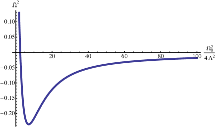
Figure 1: The Lamb shift, Eq. (81), in units $4\sqrt{\pi}J_{0}^{2}\Lambda^{3}$.

.

Moreover, assuming the same spectral density as for Eq.(78) and $a-a_{0}\rightarrow\infty$, the Lamb shift can be expressed in terms of a Meijer G-function, i.e.

$$\tilde{\Omega}^{2} = -2\int_{0}^{\infty}d\tau\int_{0}^{\infty}d\omega J(\omega)\sin\omega\tau\cos\Omega_{0}\tau$$ (81)

$$= 4\sqrt{\pi}J_{0}^{2}\Lambda^{3}{\rm G}_{13}^{21}\left(\begin{array}[]{lll}0\\ 0,3,\frac{1}{2}\end{array}\bigg{|}\frac{\Omega_{0}^{2}}{4\Lambda^{2}}\right),$$

which is depicted in Fig. 1. For an environment made up of baby universes, $\frac{\Omega_{0}}{\Lambda}\gg 1$ and the Lamb shift turns out to be very small. However, for an environment of parent universes, $\Omega_{0}\sim\Lambda$ and the corresponding Lamb shift can be of order of the original frequency, resulting then in an effective value of the energy density of the universe very closed to zero.

The multiverse of parent universes turns out to be then more effective for both the decoherence between two branches and the reduction of the theoretical value of the vacuum energy density of our universe.

III.4 Thermodynamical quantities

As a consequence of the interaction of a single universe with an environment made up of baby or parent universes, the universe undergoes an effectively non-unitary evolution determined by the three last terms of the master equation (42). As a simple example, let us take the value $q=1$, so that $D\propto(a-a_{0})$, $\gamma\propto(a-a_{0})^{3}$, and $f\propto(a-a_{0})^{2}$. For a small value of the interval $\Delta a\equiv a-a_{0}$, we can consider only the decoherence factor $D(a)$. The master equation (42) can be written then, in the configuration space, as

$$\partial_{a}\rho_{P}(\Phi,\Phi^{\prime},a)=\{-\frac{i}{2}\left(\frac{\partial^{2}}{\partial\Phi^{\prime 2}}-\frac{\partial^{2}}{\partial\Phi^{2}}\right)-\frac{i\Omega^{2}(a)}{2}(\Phi^{2}-\Phi^{\prime 2})-D(a)(\Phi-\Phi^{\prime})^{2}\}\rho_{P}(\Phi,\Phi^{\prime},a),$$ (82)

with, $D(a)\approx c_{2}(a-a_{0})$, where $c_{2}$ is given by Eqs. (57,63,67,71,77) for the different kinds of interactions considered in this section, and $\Omega(a)\approx\Omega_{ef}(a_{0})$. The master equation (82) can be solved with the Gaussian ansatz Joos et al. (2003); Schlosshauer (2007),

$$\rho(\Phi,\Phi^{\prime},a)=e^{-A(a)(\Phi-\Phi^{\prime})^{2}-iB(a)(\Phi^{2}-\Phi^{\prime 2})-C(a)(\Phi+\Phi^{\prime})^{2}-N(a)}.$$ (83)

The coefficients $A(a)$, $B(a)$ and $C(a)$ satisfy then the following differential equations Joos et al. (2003) ($N$ is a normalization factor),

$$\dot{A} = 4AB+D(a),$$ (84)

$$\dot{B} = 2B^{2}-8AC+\frac{1}{2}\Omega^{2},$$ (85)

$$\dot{C} = 4BC.$$ (86)

In order to analyze the decoherence effects of the environment on the universe, let us consider a separable initial state for the distinguished universe, i.e. a pure state, given by Schlosshauer (2007)

$$\rho(\Phi,\Phi^{\prime},a_{0})=(\frac{1}{2\pi b^{2}})^{\frac{1}{2}}e^{-\frac{\Phi^{2}+\Phi^{\prime 2}}{4b^{2}}}.$$ (87)

In that case, the initial conditions for the coefficients $A(a)$, $B(a)$ and $C(a)$ are $A(a_{0})=C(a_{0})=\frac{1}{8b^{2}}$, and $B(a_{0})=0$. With the assumption, $\Delta a\ll 1$, and disregarding higher orders than $\Delta a$, it is obtained (see, App. A2 in Ref. Joos et al. (2003))

$$A(a-a_{0}) \approx \frac{1}{8}(1+16C_{0}(a-a_{0})),$$ (88)

$$B(a-a_{0}) \approx \frac{C_{0}}{\Omega_{0}^{2}}(a-a_{0}),$$ (89)

$$C(a-a_{0}) \approx \frac{1}{8},$$ (90)

where, $C_{0}=\Omega_{0}^{4}-\frac{c_{2}}{8}$ (with, $b=1$). These coefficients allow us to obtain the thermodynamical properties of the parent universe. For instance, the purity of the state, $\zeta$, is given by Schlosshauer (2007)

$$\zeta(a-a_{0})=\sqrt{\frac{C(a)}{A(a)}}\approx\frac{1}{\sqrt{1+16C_{0}(a-a_{0})}}.$$ (91)

The linear entropy Joos et al. (2003), $S_{lin}\equiv{\rm Tr}(\rho-\rho^{2})$, turns out to be

$$S_{lin}=1-\zeta\approx 1-\frac{1}{\sqrt{1+16C_{0}(a-a_{0})}},$$ (92)

and the entropy of the distinguished universe, which for the initial state is zero as corresponds to a pure state (see, Eq. (87)), grows up due to the interaction with the environment according to

$$S=-\frac{1}{p_{0}}(p_{0}\ln p_{0}+q_{0}\ln q_{0}),$$ (93)

where Joos et al. (2003),

$$p_{0} = \frac{2\zeta}{1+\zeta},$$ (94)

$$q_{0} = \frac{1-\zeta}{1+\zeta}.$$ (95)

The linear entropy and the entropy given by Eqs. (92) and (93), respectively, are depicted in Fig. 2 in units for which $C_{0}=1$, so that it is qualitatively valid for all the kinds of interactions and environments considered in this section. The interaction between the parent universe and environment (made up of baby or parent universes) makes the state of the universe to evolve into a mixed state. That means that there exists a loss of information in the state of the distinguished universe as a consequence of the interaction with the quantum fluctuations of the space-time or with other universes of the multiverse. That loss of information makes the different branches of the universe to lose their quantum coherence and, together with other decoherence processes, leads to the feature that the universe can be described in terms of the semiclassical branch which we live in. It is worth noticing that such a loss of information appears as a result of the trace operation of the degrees of freedom that corresponds to the environment. The total system, formed by the parent universe and the rest of universes (baby or parent), retains all the information of the system along the evolution of the multiverse.

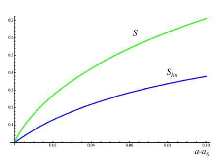
Figure 2: Entropy and linear entropy of the state of a parent universe which is interacting with a plasma of baby universes, for a linear interaction (see, Eqs. (92-93)).

IV Conclusions

The interaction between the scale factor and a scalar field with mass is seen to decohere the expanding and contracting branches of a geometrically flat, homogeneous and isotropic universe, whose expansion (or contraction) is accelerated. The decoherence turns out to be more effective in the case of a universe dominated by a quintessence fluid than when a vacuum or a phantom dominated universe are considered. This might be related to the crystal-clearer quantum nature of the latter universes.

The interaction of a parent universe with the environment, being this formed by a multiverse of parent or baby universes, can be analyzed following a parallel development to what is usually made in quantum optics. Within the approximations considered in this paper, the squeezed vacuum state and the thermal state of baby universes produce similar effects provided that the squeezing of the state of baby universes be interpreted as an effective creation of a high number of fluctuations, i.e. for a large squeezing effect.

The linear interaction produces leading terms in the change of the properties of the parent universe, being therefore subdominant the effects of the quadratic interaction. However, it does not imply that the quadratic interaction has no relevant effects on the state of the parent universe because it is actually the responsible for the change of the high order coherence properties of the fields that propagate upon the space-time González-Díaz (1992a).

The distinguished universe undergoes an effectively non-unitary evolution as due to the interaction with the environment. The decoherence and dissipation effects are even more acute if the environment is taken to be a multiverse made up of parent universes, because their energy density is assumed to be of the order of that for the distinguished parent universe.

Much as it happens with the Lamb shift in quantum mechanics, here the vacuum energy of the distinguished universe is also shifted. In the case of an environment made up of baby universes, which can be considered to be similar to that previously studied by Coleman Coleman (1988a), the corresponding Lamb shift is important for a large squeezing effect or a large number of vacuum fluctuations. The effect is greater if the environment is a multiverse of parent universes since the corresponding Lamb shift matches the theoretical predictions for the vacuum energy of a single universe. That could effectively reduce the value of the energy density of the universe to be very closed to zero even for the interaction between the parent universe with the fluctuations of its ground state.

Moreover, the entropy of the distinguished universe grows as a consequence of the interaction with its environment. Such an irreversible interaction may provide us then with an arrow of time.

References

- Kiefer (2007) C. Kiefer, Quantum gravity (Oxford University Press, Oxford, UK, 2007).
- Joos et al. (2003) E. Joos et al., Decoherence and the Appearance of a Classical World in Quantum Theory (Springer-Verlag, Berlin, Germany, 2003).
- Zeh (1986) H. D. Zeh, Phys. Lett. A 116, 9 (1986).
- Halliwell (1989) J. J. Halliwell, Phys. Rev. D 39, 2912 (1989).
- Kiefer (1992) C. Kiefer, Phys. Rev. D 46, 1658 (1992).
- Coleman (1988a) S. Coleman, Nucl. Phys. B 307, 867 (1988a).
- Coleman (1988b) S. Coleman, Nucl. Phys. B 310, 643 (1988b).
- González-Díaz (1992a) P. F. González-Díaz, Phys. Rev. D 45, 499 (1992a).
- Halliwell and Hawking (1985) J. J. Halliwell and S. W. Hawking, Phys. Rev. D 31, 1777 (1985).
- González-Díaz and Robles-Pérez (2009) P. F. González-Díaz and S. Robles-Pérez, Phys. Lett. B 679, 298 (2009).
- González-Díaz and Robles-Pérez (2008) P. F. González-Díaz and S. Robles-Pérez, Int. J. Mod. Phys. D 17, 1213 (2008), eprint 0709.4038.
- Robles-Pérez and González-Díaz (2010) S. Robles-Pérez and P. F. González-Díaz, Phys. Rev. D 81, 083529 (2010), eprint arXiv:1005.2147v1.
- Vilenkin (1986) A. Vilenkin, Phys. Rev. D 33, 3560 (1986).
- Abramovitz and Stegun (1972) M. Abramovitz and I. A. Stegun, eds., Handbook of Mathematical Functions (NBS, 1972).
- Dabrowski et al. (2006) M. P. Dabrowski et al., Phys. Rev. D 74, 044022 (2006).
- Nojiri and Odintsov (2004) S. Nojiri and S. D. Odintsov, Phys. Rev. D 70, 103522 (2004).
- Sushkov (2005) S. Sushkov, Phys. Rev. D 71, 043520 (2005).
- Lobo (2005) F. S. N. Lobo, Phys. Rev. D 71, 084011 (2005).
- González-Díaz (2003) P. F. González-Díaz, Phys. Rev. D 68, 084016 (2003).
- Strominger (1990) A. Strominger, in Quantum Cosmology and Baby Universes, edited by S. Coleman, J. B. Hartle, T. Piran, and S. Weinberg (World Scientific, London, UK, 1990), vol. 7.
- Lewis and Riesenfeld (1969) H. R. Lewis and W. B. Riesenfeld, J. Math. Phys. 10, 1458 (1969).
- Wheeler (1957) J. A. Wheeler, Ann. Phys. 2, 604 (1957).
- Grishchuk and Sidorov (1990) L. P. Grishchuk and Y. V. Sidorov, Phys. Rev. D 42, 3413 (1990).
- Khandekar and Lawande (1986) D. C. Khandekar and S. V. Lawande, Phys. Rep. 137, 115 (1986).
- Mukhanov and Winitzki (2007) V. F. Mukhanov and S. Winitzki, Quantum Effects in Gravity (Cambridge University Press, Cambridge, UK, 2007).
- Vergel and Villaseñor (2009) D. G. Vergel and J. S. Villaseñor, Ann. Phys. 324, 1360 (2009).
- Farhi and Guth (1987) E. Farhi and A. H. Guth, Phys. Lett. B 183, 149 (1987).
- Giddings and Strominger (1988) S. B. Giddings and A. Strominger, Nucl. Phys. B 207, 854 (1988).
- González-Díaz (1992b) P. F. González-Díaz, Phys. Lett. B 293, 294 (1992b).
- Schlosshauer (2007) M. Schlosshauer, Decoherence and the quantum-to-classical transition (Springer, Berlin, Germany, 2007).
- Garay (1998) L. J. Garay, Phys. Rev. D 58, 124015 (1998).
- Kiefer and Polarski (1998) C. Kiefer and D. Polarski, Ann. Phys. 7, 137 (1998).