Global Neutrino Data Analysis and the Quest to Pin Down
$\sin\theta_{13}$ in Different Mixing Matrix Parametrizations

Abstract

Hints for sizable $\sin^{2}\theta_{13}$ have been reported in earlier global neutrino oscillation data analyses as well as will be reported in this work, and quite recently by the Double Chooz experiment. However, as we enter the era of precision neutrino oscillation experiments, terms linear in $\sin\theta_{13}$ will no longer be negligible, and its sign would affect the extraction of other oscillation parameters. The sign of $\sin\theta_{13}$ also plays a crucial role in the determination of the CP-violating phase. In this work we show that by adopting an alternative parametrization for the Pontecorvo-Maki-Nakagawa-Sakata (PMNS) mixing matrix, one already has a chance to infer the sign of each mixing angle in the conventional parametrization using existing global neutrino data. A weak preference for negative $\sin\theta_{13}$ is found. In particular, the solar data suggest that $\sin\theta_{13}>0$ while all other data the opposite. This leads to the speculation on whether the Mikheyev-Smirnov-Wolfenstein (MSW) effect is responsible. In this work we found that in the new mixing matrix parametrization, the $68\%$ CL constraints on the three mixing angles are comparable to those estimated in the conventional parametrization adopted in the literature. Owing to the strong correlations among the three mixing angles in the new parametrization, the advantages of doing the global neutrino oscillation analysis using data from past, current, and near future neutrino oscillation experiments shall become manifest.

I Introduction

The experiments involving solar, reactor, atmospheric and accelerator neutrinos have established a picture of neutrino oscillations caused by non-zero neutrino masses and mixing among different neutrino flavors (see e.g. Ref. [1]). The phenomenology of neutrino oscillations arising from the mismatch between the weak and the mass eigenstates can be described by the Pontecorvo-Maki-Nakagawa-Sakata (PMNS) mixing matrix [2, 3]. This matrix can be parametrized in various ways as seen in the literature (e.g., [4, 5, 6, 7, 8, 9]).

All experimental data except those from the LSND [10] can be well described assuming three active neutrinos. In the case of Dirac neutrinos, the $3\times 3$ unitary mixing matrix is characterized by three Euler angles and one physical phase, and can be expressed as a product of three rotation matrices. The physical phase can be responsible for CP violation in the neutrino sector. As mentioned in Ref. [5], the CP-violating phase can be associated with the sine or cosine of any mixing angle or with the identity entry in any of the three rotation matrices. In this work, we will follow the standard Cabibbo-Kobayashi-Maskawa (CKM) matrix [11] for the assignment of the CP-violating phase.

Define

$$R_{23}=\left(\begin{array}[]{ccc}1&0&0\\ 0&c_{23}&s_{23}\\ 0&-s_{23}&c_{23}\end{array}\right),\hskip 14.22636ptR_{13}=\left(\begin{array}[]{ccc}c_{13}&0&s_{13}\\ 0&1&0\\ -s_{13}&0&c_{13}\end{array}\right),\vspace{-0.3cm}$$

$$R_{12}=\left(\begin{array}[]{ccc}c_{12}&s_{12}&0\\ -s_{12}&c_{12}&0\\ 0&0&1\end{array}\right),\vspace{-0.3cm}$$ (1)

and

$$W_{23}=\left(\begin{array}[]{ccc}1&0&0\\ 0&c_{23}&s_{23}e^{-i\delta_{cp}}\\ 0&-s_{23}e^{i\delta_{cp}}&c_{23}\end{array}\right),\\$$

$$W_{13}=\left(\begin{array}[]{ccc}c_{13}&0&s_{13}e^{-i\delta_{cp}}\\ 0&1&0\\ -s_{13}e^{i\delta_{cp}}&0&c_{13}\end{array}\right),\\$$

$$W_{12}=\left(\begin{array}[]{ccc}c_{12}&s_{12}e^{-i\delta_{cp}}&0\\ -s_{12}e^{i\delta_{cp}}&c_{12}&0\\ 0&0&1\end{array}\right),$$ (2)

where $\theta_{ij}$ and $\delta_{cp}$ are the mixing angles and the CP-violating phase, respectively, $c_{ij}\equiv\cos\theta_{ij}$ and $s_{ij}\equiv\sin\theta_{ij}$. As the combination $R_{23}W_{13}R_{12}$ is the standard choice for describing the quark mixing, it has been adopted to be the conventional parametrization for the mixing matrix for Dirac neutrinos. This choice of the parametrization was actually made prior to the era when neutrino oscillation data became available. Later, the solar neutrino experiments [12, 13, 14, 15], reactor [16, 17], long-baseline (LBL) accelerator [18, 19, 20], as well as the atmospheric neutrino experiments [21, 22, 23] all choose this parametrization to present their results. Using existing global neutrino data, most phenomenology works [24, 25, 26, 27, 28, 29, 30, 31] also employ this parametrization to determine neutrino oscillation parameters.

In the conventional parametrization, the three mixing angles happen to nearly decouple for solar, atmospheric/accelerator, and reactor neutrino oscillation experiments due to the different neutrino energies and traveling distances involved. The $\theta_{12}$ and $\theta_{23}$ angles are well determined by solar and atmospheric experiments, respectively. Current-generation short-baseline reactor experiments such as the Daya Bay [32], Double Chooz [33], RENO [34] and the Angra [35] experiments are exploited to pin down the yet unknown $\theta_{13}$ value. Non-zero or sizable $\theta_{13}$ values are predicted by many neutrino mass models (see e.g. Ref. [36] for a nice compilation of existing model predictions), and supported by global neutrino data analyses (see e.g. Ref [24, 25, 26, 29] and this work). Very recently, the Double Chooz experiment [37] has reported their preliminary results of $\sin^{2}2\theta_{13}=0.085\pm 0.051$ (68$\%$ CL). When this is confirmed in the future by other experiments with even better sensitivities, it will be good news for near-future experiments such as T2K [38], NO$\nu$A [39], T2HK [40], T2KK [41]. Their goal of measuring the CP-violating effect will be more reachable.

This is not the end of the story for the neutrino oscillation community. Another issue is the determination of the sign of $\sin\theta_{13}$. As we enter the era of precision neutrino oscillation experiments, terms linear in $\sin\theta_{13}$ may no longer be negligible in fitting the mixing angles. From the Jarlskog invariant quantity [42, 43] of CP violation, one sees that the sign of $\sin\theta_{13}$ would also have an impact on the $\delta_{cp}$ determination. However, in the conventional parametrization, the reactor and solar experiments are only sensitive to $\sin^{2}\theta_{13}$. For LBL accelerator or atmospheric experiments, the observable has terms linear in $\sin\theta_{13}$, but only sub-dominant. Despite the unfavorable situation one faces when working in the conventional parametrization, a first attempt to determine the sign of $\sin\theta_{13}$ has been made in Ref. [27] using the LBL accelerator, CHOOZ, and atmospheric neutrino data.

In fact the conventional parametrization is not the only way to establish the mixing matrix. As proposed by several authors [4, 5, 8, 7, 6, 9], the corresponding mixing parameters may be more accessible, without sacrificing accuracy, in other parametrizations. In this work we follow the approach of Ref. [9] to explore this possibility. Besides the conventional parametrization, we perform a global neutrino oscillation analysis adopting an alternative parametrization, $R_{13}W_{12}R_{23}$, in which the observables have leading terms linear in any of the three mixing angles. Equipped with the analysis results obtained in these two parametrizations, we will be eligible to address a couple of issues. Can one determine the sign of $\sin\theta_{13}$? Are there other parametrizations which can provide comparable sensitivities in extracting neutrino oscillation parameters as the conventional one? How are the three mixing angles correlated with each other therein? Do the matter (MSW) effects [44, 45] affect the sign of $\sin\theta_{13}$?

This paper is organized as follows. In Section II we briefly describe our data fitting procedure in the conventional parametrization (to be denoted by $\mathcal{A}$). In Section III we present and discuss our results obtained from a similar analysis done in an alternative parametrization (to be denoted by $\mathcal{D}$). Section IV gives our summary and outlook. Individual analysis approaches for each neutrino oscillation experiment are detailed in Appendix A through D.

II Analysis

Table I in Ref. [9] indicates that the predicted neutrino mixing angles in the parametrizations $R_{23}W_{13}R_{12}$, $R_{23}W_{12}R_{13}$, and $R_{13}W_{23}R_{12}$ come up with similar values, while those in $R_{13}W_{12}R_{23}$, $R_{12}W_{23}R_{13}$, and $R_{12}W_{13}R_{23}$ end up with similar values. We thus preform a global fit of the neutrino mixing parameters using parameterizations $R_{23}W_{13}R_{12}$ and $R_{13}W_{12}R_{23}$, taking advantage of the fact that these two parameterizations will have dissimilar outcomes. Following Ref. [9], we denote them as the $\mathcal{A}$ and $\mathcal{D}$ ’representations’ respectively, where representation $\mathcal{A}$ corresponds to the conventional mixing matrix parametrization. In what follows, notations ($\Delta^{\mathcal{A}}m^{2}_{ij}$, $\theta^{\mathcal{A}}_{ij}$) and ($\Delta^{\mathcal{D}}m^{2}_{ij}$, $\theta^{\mathcal{D}}_{ij}$) stand for the oscillation parameters directly determined using representations $\mathcal{A}$ and $\mathcal{D}$, respectively. On the other hand, the notation $\theta^{\mathcal{DA}}_{ij}$ symbolizes the three mixing angles that are initially extracted from representation $\mathcal{D}$ and then translated to representation $\mathcal{A}$ by the transformation method described in Ref. [9]. The transformation from representation $\mathcal{D}$ to $\mathcal{A}$ is outlined in Appendix E.

The global neutrino data used in this work include (i) solar data from rates measured in chlorine [46] and gallium [47] experiments, the rate of ⁷Be solar neutrinos measured in the Borexino [48] experiment, Super-Kamiokande (SK) phase I & II day/night spectra [14, 15], and SNO phases I & II $\nu_{e}$ survival probability [12]; (ii) reactor data from KamLAND [16] and CHOOZ [17]; (iii) LBL accelerator data from K2K [18] and MINOS $\nu_{\mu}$ disappearance channel [19] and $\nu_{e}$ appearance channel [20]; and (iv) atmospheric data from SK phase I [23] and SNO [22].

In this work, the re-evaluated $\bar{\nu}_{e}$ flux from nuclear power plants [49] is not taken into consideration for the reactor data. In addition, the large number of bins in the atmospheric data of SK phases II and III, as well as the lack of information, prevents us from reproducing their results. Therefore we do not include the SK-II and SK-III atmospheric data in our work. Since our purpose is to investigate the neutrino mixing phenomenology in different parametrizations using the same data sets and analysis conditions, the absence of these factors should not have any impact on the conclusions of this work. Described below is our analysis of the global neutrino data.

Appendix A outlines the analyses for each solar experiment employed in this work which includes chlorine, gallium, Borexino, SK and SNO. We use the Bahcall solar neutrino spectra [50] except for the ⁸B neutrino spectrum, which is from Ref. [51]. Neutrino survival probabilities in the Sun are estimated using the BS05(OP) model [52] for the neutrino production rates at different solar radii. We do not use the more recent BPS09(GS) or BPS09(AGSS09) models [53] because of the conservative model uncertainties. For estimating neutrino survival probabilities inside the Earth, the Earth density profile of PEM-C [54] (rather than PREM [55]) is adopted in this work. It assumes the continental crust for the outer most layer of the Earth where the solar neutrinos enter the detectors. In our analysis, the flux of ⁸B solar neutrinos is a nuisance parameter while the fluxes of other solar neutrinos are taken from the BS05 model [52]. Neutrino oscillation probabilities are calculated using the adiabatic approximation [56]. It has been verified to yield equivalent results as the numerical calculation does for several sets of neutrino oscillation parameters in the LMA region.

Our analyses of oscillation parameter fitting using the KamLAND and the CHOOZ $\bar{\nu}_{e}$ oscillation events are delineated in Appendix B. Owing to the short distances between the source and the detector, matter effects are generally insignificant and oscillation probabilities in vacuum suffice. This is also the case for accelerator neutrino analyses. Appendix C describes the analyses of oscillation parameter fitting using the K2K and the MINOS $\nu_{\mu}$ disappearance channel as well as the MINOS $\nu_{e}$ appearance channel.

Atmospheric neutrino data from the SK [23] and the SNO [22] experiments are included in our analysis as described in Appendix D. We first employ the NUANCE package [57] to simulate atmospheric neutrino events assuming no oscillation effects. Neutrino oscillations in the atmosphere and inside the Earth are then incorporated by the ”weighting factors”, Eq. (21), with the matter effects taken into account by following the prescription of Ref. [58]. We apply similar criteria and cuts on the kinematics of the simulated events so that we achieve the same selection efficiency as Ref. [23] does for SK atmospheric data and as Ref. [22] does for SNO atmospheric data.

Data Sample	$|{\Delta^{\mathcal{A}}m^{2}_{21}}|$	$|\Delta^{\mathcal{A}}m^{2}_{32}|$	$\theta^{\mathcal{A}}_{12}$	$\theta^{\mathcal{A}}_{23}$	$|\theta^{\mathcal{A}}_{13}|$
	[$10^{-5}$ eV2]	[$10^{-3}$ eV2]	[$\tan^{2}\theta^{\mathcal{A}}_{12}$]	[$\sin^{2}\theta^{\mathcal{A}}_{23}$]	[$\sin^{2}\theta^{\mathcal{A}}_{13}$]
Solar-only	$6.55^{+3.21}_{-2.57}$		$33.587^{+2.156}_{-1.603}$		$5.444^{+8.735}_{-5.444}$
			[$0.441^{+0.077}_{-0.051}$]		[$0.009^{+0.051}_{-0.009}$]
KamLAND-only	$7.57^{+0.27}_{-0.22}$		$34.659^{+5.459}_{-5.010}$		$8.723^{+7.495}_{-8.723}$
			[$0.478^{+0.232}_{-0.154}$]		[$0.023^{+0.055}_{-0.023}$]
Solar+KamLAND	$7.57^{+0.26}_{-0.22}$		$34.001^{+0.881}_{-0.900}$		$9.458^{+2.651}_{-3.718}$
			[$0.455^{+0.031}_{-0.030}$]		[$0.027^{+0.020}_{-0.017}$]
Accel+Atmos		$2.30^{+0.21}_{-0.11}$		$43.739^{+4.391}_{-4.391}$	$5.132^{+3.591}_{-5.132}$
+CHOOZ				[$0.478^{+0.058}_{-0.058}$]	[$0.008^{+0.015}_{-0.008}$]
Global					$7.492^{+1.231}_{-1.753}$
$(\Delta\chi^{2}=1.0)$					[$0.017^{+0.006}_{-0.007}$]
Global					$7.492^{+1.787}_{-3.049}$
$(\Delta\chi^{2}=2.30)$					[$0.017^{+0.009}_{-0.011}$]

Table 1: Summary of our best-fit oscillation parameters, $\Delta^{\mathcal{A}}m^{2}_{ij}$ and $\theta^{\mathcal{A}}_{ij}$, in representation $\mathcal{A}$, where the mxing angles, $\theta^{\mathcal{A}}_{ij}$, are in unit of degrees. In our analysis we only fitted $\sin^{2}\theta^{\mathcal{A}}_{23}$ in the range below 0.5. In order to compare the 68$\%$ CL constraints determined in representations $\mathcal{A}$ and $\mathcal{D}$, we assume the upper and lower bounds from accelerator$+$CHOOZ$+$atmospheric data are about the same.

We first perform a global analysis using representation $\mathcal{A}$ in order to compare with existing results from the literature. As the current global neutrino data is insensitive to $\delta_{cp}$, we have selected $\delta_{cp}=0$. According to the study presented in Ref. [9], this choice also turns out to be adequate for representation $\mathcal{D}$ since a rephasing still gives $\delta_{cp}=0$ therein. Table 1 summarizes our best-fit results for the oscillation parameters from various three-flavor analyses in this case. Assuming CPT invariance, the results from the KamLAND reactor experiment and all solar experiments are combined in the $\chi^{2}$ function: $\chi^{2}_{\rm sol+KL}\equiv\chi^{2}_{\rm solar}+\chi^{2}_{\rm KL}$. We minimize $\chi^{2}_{\rm sol+KL}$ with respect to the oscillation parameters $\Delta^{\mathcal{A}}m^{2}_{21}$, $\tan^{2}\theta^{\mathcal{A}}_{12}$, and $\sin^{2}\theta^{\mathcal{A}}_{13}$, as well as the ⁸B solar neutrino flux in a three-flavor hypothesis. The other two parameters are fixed at $\Delta^{\mathcal{A}}m^{2}_{32}=2.4\times 10^{-3}$ eV² and $\sin^{2}\theta^{\mathcal{A}}_{23}=0.5$. The best-fit values are found to agree with the results presented in Refs. [12, 16]. Figure 1 shows the allowed regions in the planes of ($\tan^{2}\theta^{\mathcal{A}}_{12}$, $\Delta^{\mathcal{A}}m^{2}_{21}$), ($\sin^{2}\theta^{\mathcal{A}}_{13}$, $\Delta^{\mathcal{A}}m^{2}_{21}$), and ($\tan^{2}\theta^{\mathcal{A}}_{12}$, $\sin^{2}\theta^{\mathcal{A}}_{13}$).

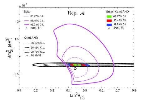
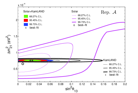
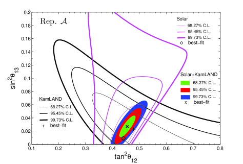
Figure 1: Results of the solar and KamLAND oscillation parameter analysis in a three-flavor hypothesis performed in representation $\mathcal{A}$, where $\Delta^{\mathcal{A}}m^{2}_{32}=2.4\times 10^{-3}$ eV² and $\sin^{2}\theta^{\mathcal{A}}_{13}=0.5$ are assumed.

The $\chi^{2}$ functions for K2K, MINOS $\nu_{\mu}$ disappearance, MINOS $\nu_{e}$ appearance, CHOOZ, as well as SK and SNO atmospheric neutrino data are also summed together: $\chi^{2}_{\rm acc+CHOOZ+atm}\equiv\chi^{2}_{\rm acc}+\chi^{2}_{\rm CHOOZ}+\chi^{2}_{\rm atm}$. By minimizing this $\chi^{2}$ with respect to the oscillation parameters $\Delta^{\mathcal{A}}m^{2}_{32}$, $\sin^{2}\theta^{\mathcal{A}}_{23}$, and $\sin^{2}\theta^{\mathcal{A}}_{13}$ while fixing $\Delta^{\mathcal{A}}m^{2}_{21}=7.67\times 10^{-5}$ eV² and $\tan^{2}\theta^{\mathcal{A}}_{12}=0.427$, and assuming a normal mass hierarchy, the best-fit values are found to be consistent with the most recent results in Ref. [25, 24]. Figure 2 shows the likelihood contours in the planes of ($\sin^{2}\theta^{\mathcal{A}}_{23}$, $\Delta^{\mathcal{A}}m^{2}_{32}$), ($\sin^{2}\theta^{\mathcal{A}}_{13}$, $\Delta^{\mathcal{A}}m^{2}_{32}$), and ($\sin^{2}\theta^{\mathcal{A}}_{23}$, $\sin^{2}\theta^{\mathcal{A}}_{13}$).

Finally, for individual data sample mentioned above, i.e. the solar-only, KamLAND, solar$+$KamLAND, and accelerator$+$CHOOZ$+$atmospheric, the differences ($\Delta\chi^{2}$) between $\chi^{2}$ and the minimum $\chi^{2}_{\rm min}$ as a function of $\sin^{2}\theta^{\mathcal{A}}_{13}$ are obtained by marginalizing the other two oscillation parameters. Our results are shown in Fig. 3 for $\Delta\chi^{2}_{\rm solar}$, $\Delta\chi^{2}_{\rm KL}$, $\Delta\chi^{2}_{\rm sol+KL}$ and $\Delta\chi^{2}_{\rm acc+CHOOZ+atm}$. The global result is then

$$\Delta\chi^{2}_{\rm global}(\sin^{2}\theta^{\mathcal{A}}_{13})\equiv\Delta\chi^{2}_{\rm sol+KL}+\Delta\chi^{2}_{\rm acc+CHOOZ+atm}\,.$$ (3)

Our result for $\sin^{2}\theta^{\mathcal{A}}_{13}$ is consistent with those from other global neutrino data analyses (e.g., [12, 16, 24, 25, 26]). We also find a weak hint for non-zero $\sin^{2}\theta^{\mathcal{A}}_{13}$ at 95$\%$ CL, but it is not easy to determine the sign of $\sin\theta^{\mathcal{A}}_{13}$.

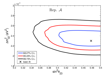
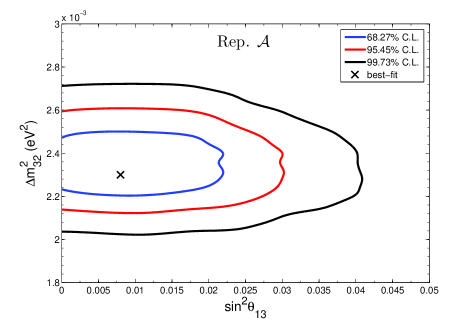
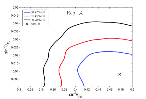
Figure 2: Three-flavor oscillation parameter results in representation $\mathcal{A}$ for the combined analysis of the LBL accelerator, CHOOZ, and atmospheric data sets, where the parameters $\Delta^{\mathcal{A}}m^{2}_{21}=7.67\times 10^{-5}$ eV² and $\tan^{2}\theta^{\mathcal{A}}_{12}=0.427$ are assumed.

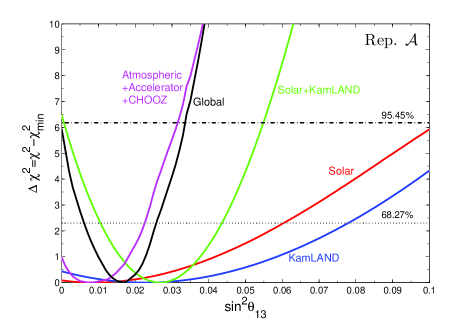
Figure 3: $\Delta\chi^{2}$ as a function of $\sin^{2}\theta^{\mathcal{A}}_{13}$ for various combinations of oscillation data where the undisplayed parameters are floated.

III Results and Discussions

Changing to representation $\mathcal{D}$ and fixing $\delta_{cp}=0$, we perform a similar $\chi^{2}$ analysis as that in previous section using exactly the same data sets. After determining the oscillation parameters $\Delta^{\mathcal{D}}m^{2}_{ij}$ and $\theta^{\mathcal{D}}_{ij}$, with the transformation strategy described in Appendix E, we also perform a translation of the best-fit mixing angles back to representation $\mathcal{A}$, denoted by $\theta^{\mathcal{DA}}_{ij}$. Both results are given in Table 2 for a comparison with the corresponding $\Delta^{\mathcal{A}}m^{2}_{ij}$ and $\theta^{\mathcal{A}}_{ij}$ retrieved directly in representation $\mathcal{A}$.

Data Sample	$|{\Delta^{\mathcal{D}}m^{2}_{21}}|$	$|\Delta^{\mathcal{D}}m^{2}_{32}|$	$\theta^{\mathcal{D}}_{12}$	$\theta^{\mathcal{D}}_{23}$	$\theta^{\mathcal{D}}_{13}$	$\theta^{\mathcal{D}}_{12}$	$\theta^{\mathcal{D}}_{23}$	$\theta^{\mathcal{D}}_{13}$
	[$10^{-5}$ eV2]	[$10^{-3}$ eV2]	[$\theta^{\mathcal{DA}}_{12}$	$\theta^{\mathcal{DA}}_{23}$	$\theta^{\mathcal{DA}}_{13}$]	[$\theta^{\mathcal{DA}}_{12}$	$\theta^{\mathcal{DA}}_{23}$	$\theta^{\mathcal{DA}}_{13}$]
			Global Minimum			Second Minimum
Solar-only	$6.00^{+3.20}_{-2.60}$		25.0	57.0	-24.0
			[33.662	49.827	5.870]
KamLAND-only	$7.60^{+0.23}_{-0.25}$		36.0	50.0	-46.0
			[55.362	38.814	-8.604]
Solar+KamLAND	$7.60^{+0.23}_{-0.25}$		11.0	57.0	-34.0
			[34.300	56.689	-9.898]
Accel+Atmos		$2.40^{+0.18}_{-0.12}$	27.0	50.0	-38.0
+CHOOZ			[44.978	43.445	-6.990]
Global	7.6	2.4	$19.0^{+1.8}_{-3.2}$	$46.0^{+4.6}_{-4.0}$	$-29.0^{+1.5}_{-2.5}$	$28.5^{+2.0}_{-2.5}$	$51.5^{+3.5}_{-4.5}$	$-20.0^{+2.5}_{-2.0}$
$(\Delta\chi^{2}=2.30)$			[33.461	43.326	$-7.582$]	[33.509	43.980	7.932]
			[$\pm$0.891	$\pm$4.391	$\pm$2.418]	[$\pm$1.760	$\pm$4.118	$\pm$2.502]

Table 2: Summary of our best-fit oscillation parameters, $\Delta^{\mathcal{D}}m^{2}_{ij}$ and $\theta^{\mathcal{D}}_{ij}$, in representation $\mathcal{D}$, and the translated mixing angles, $\theta^{\mathcal{DA}}_{ij}$ in representation $\mathcal{A}$, where all of the mixing angles are in unit of degrees. Note that the 68$\%$ CL constraints of the best-fit results from the second minimum is taken at $\Delta\chi^{2}=\chi^{2}-\chi^{2}_{min}=2.3$ with $\chi^{2}_{min}$ being the $\chi^{2}$ value at the second minimum. The uncertainties of $\theta^{\mathcal{DA}}_{ij}$ are listed at the last row.

We found that in representation $\mathcal{D}$, individual data sets, i.e. the global solar data, KamLAND, solar$+$KamLAND, and the combined accelerator$+$CHOOZ$+$atmospheric data, cannot constrain the three mixing angles well. However, when combined altogether, they infer bounds at 68$\%$ confidence level (CL) on the three mixing angles $\theta^{\mathcal{D}}_{ij}$ which are comparable to those on $\theta^{\mathcal{A}}_{ij}$ (cf. Table 2), except for $\theta^{\mathcal{D}}_{12}$. We therefore give only the bounds obtained from the combined global neutrino data.

Using the global solar data, we find that the best-fit values of $\theta^{\mathcal{DA}}_{12}$ and $\theta^{\mathcal{DA}}_{13}$ are consistent with those of $\theta^{\mathcal{A}}_{12}$ and $\theta^{\mathcal{A}}_{13}$, respectively. In representation $\mathcal{A}$, the solar data are not sensitive to $\theta^{\mathcal{A}}_{23}$, thus one should not naively compare the translated best-fit result of $\theta^{\mathcal{DA}}_{23}\sim 50^{\circ}$ to the input value of $\theta^{\mathcal{A}}_{23}=45^{\circ}$. The KamLAND data are insensitive to $\theta^{\mathcal{A}}_{23}$ too and have less constraining power on $\theta^{\mathcal{A}}_{12}$. These two facts explain why the translated values of $\theta^{\mathcal{DA}}_{12}$ and $\theta^{\mathcal{DA}}_{23}$ are very different from the expected values, $\theta^{\mathcal{A}}_{12}$ and $\theta^{\mathcal{A}}_{23}$. Surprisingly, the translated best-fit $\theta^{\mathcal{DA}}_{13}$ turns out to be almost the same as $\theta^{\mathcal{A}}_{13}$ in magnitude, but with an opposite sign. Like the KamLAND-only results, the combined solar and KamLAND results produce best-fit values where $\theta^{\mathcal{DA}}_{12}\sim\theta^{\mathcal{A}}_{12}$ and $|\theta^{\mathcal{DA}}_{13}|\sim|\theta^{\mathcal{A}}_{13}|$, and $\theta^{\mathcal{DA}}_{13}<0$.

Similarly, combining the LBL accelerator, CHOOZ, and atmospheric neutrino data, the translated best-fit $\theta^{\mathcal{DA}}_{23}$ and $|\theta^{\mathcal{DA}}_{13}|$ are consistent with the best-fit $\theta^{\mathcal{A}}_{23}$ and $|\theta^{\mathcal{A}}_{13}|$, respectively. The combined accelerator$+$CHOOZ$+$atmospheric data are not sensitive to $\theta^{\mathcal{A}}_{12}$, so a comparison of the best-fit value of $\theta^{\mathcal{DA}}_{12}\sim 45^{\circ}$ with the input value of $\theta^{\mathcal{A}}_{12}=33.2^{\circ}$ is not necessary. Interestingly for this case, it was found that the best fit $\theta^{\mathcal{DA}}_{13}<0$ as well. This finding has been discussed in Ref. [27] using a similar data sample.

In spite of the poor constraints on $\theta^{\mathcal{D}}_{ij}$, the parameter $\Delta^{\mathcal{D}}m^{2}_{21}$ determined by analyzing the solar, KamLAND and solar$+$KamLAND data, as well as $\Delta^{\mathcal{D}}m^{2}_{32}$ from the combined analysis of the LBL accelerator, CHOOZ and the atmospheric data agree well with those directly extracted in representation $\mathcal{A}$. Equipped with the above individual $\chi^{2}$ calculation, we perform a global analysis straightforwardly via

$$\Delta\chi^{2}_{\rm global}(\theta^{\mathcal{D}}_{12},\theta^{\mathcal{D}}_{23},\theta^{\mathcal{D}}_{13})\equiv\Delta\chi^{2}_{\rm sol+KL}+\Delta\chi^{2}_{\rm acc+CHOOZ+atm}\,.$$ (4)

Here we fix $\Delta^{\mathcal{D}}m^{2}_{21}=7.6\times 10^{-5}$ eV² and $\Delta^{\mathcal{D}}m^{2}_{32}=2.4\times 10^{-3}$ eV², the best-fit values determined from the solar$+$KamLAND and the acc$+$CHOOZ$+$atm analysis, respectively. Our results at 68$\%$ CL are given in Table 2, and Fig. 4 shows the projected likelihood contour plots in the planes of $(\theta^{\mathcal{D}}_{12},\theta^{\mathcal{D}}_{13})$, $(\theta^{\mathcal{D}}_{23},\theta^{\mathcal{D}}_{13})$, and $(\theta^{\mathcal{D}}_{12},\theta^{\mathcal{D}}_{23})$. As already advertised in the beginning of this section, we find that the 68$\%$ CL constraints on $\theta^{\mathcal{D}}_{ij}$ are comparable to those on $\theta^{\mathcal{A}}_{ij}$, with the exception of $\theta^{\mathcal{D}}_{12}$.

Sign of $\sin\theta^{\mathcal{A}}_{13}$

As we enter the era of precision neutrino oscillation experiments, terms linear in $\sin\theta_{13}$ can no longer be neglected. As pointed out in Ref. [27], it will be necessary to perform a parameter fitting in the $\sin\theta^{\mathcal{A}}_{13}<0$ regime as well. The sign of $\sin\theta_{13}$ also plays the decisive role to the $\delta_{cp}$ determination. This can be seen in the Jarlskog invariant quantity of CP violation [42, 43]. For any representation $\mathcal{H}$, it is defined as

$${\mathcal{J}}=\sin 2\theta^{\mathcal{H}}_{12}\sin 2\theta^{\mathcal{H}}_{23}\sin 2\theta^{\mathcal{H}}_{13}\cos\theta^{\mathcal{H}}_{ij}\sin\delta_{cp}^{\mathcal{H}}\,,$$ (5)

where $\theta^{\mathcal{H}}_{ij}$ is the mixing angle seated in the middle of the three rotation matrices in the mixing matrix. For representation $\mathcal{H}=\mathcal{A}$ or $\mathcal{D}$, both $\sin 2\theta^{\mathcal{H}}_{12}$ and $\sin 2\theta^{\mathcal{H}}_{23}$ are positive. However, for the existing global neutrino data, the leading terms of the observables in representation $\mathcal{A}$ are linear in $\sin^{2}\theta_{13}$ while the terms linear in $\sin\theta_{13}$ are in the sub-leading terms. This makes difficult to determine the sign of $\sin\theta_{13}$ in representation $\mathcal{A}$.

An interesting feature is seen when analyzing neutrino data in representation $\mathcal{D}$. Two local minima exist in the global $\chi^{2}$, one corresponding to $\theta^{\mathcal{DA}}_{13}<0$ (the global minimum) and the other one $\theta^{\mathcal{DA}}_{13}>0$ (the second minimum). Apart from this, both minima have very similar values of $\theta^{\mathcal{DA}}_{12}$, $\theta^{\mathcal{DA}}_{23}$, and $|\theta^{\mathcal{DA}}_{13}|$, which also agree well with the best-fit $\theta^{\mathcal{A}}_{12}$, $\theta^{\mathcal{A}}_{23}$, and $|\theta^{\mathcal{A}}_{13}|$ (cf. Table 1), respectively. This suggests that by doing global neutrino data analysis in representation $\mathcal{D}$, one has a chance to identify the sign of $\sin\theta^{\mathcal{DA}}_{13}$. In the current case, the $\chi^{2}$ values for the global minimum and the second minimum differ by $\sim$2. While this preference for negative $\sin\theta_{13}$ is weak, the inclusion of data from the current and the near-future neutrino experiments may help strengthen the evidence.

Compared among the various data samples used, the global solar data point to $\theta^{\mathcal{DA}}_{13}>0$ while all the other data $\theta^{\mathcal{DA}}_{13}<0$. We do not have the explanation for this difference yet. One may investigate whether the matter (MSW) effects [44, 45] influence the sign of $\theta^{\mathcal{DA}}_{13}$ during the propagation of solar neutrinos through the Sun and the Earth. Atmospheric neutrinos propagating through the Earth are also subject to the MSW effects (see Appendix D), but to a much less degree. This issue will be further studied in a separate work.

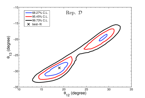
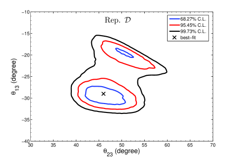
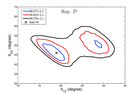
Figure 4: Three-flavor hypothesis mixing angle results for the combined analysis of global neutrino data in representation $\mathcal{D}$. The neutrino mass differences are fixed to the values $\Delta^{\mathcal{D}}m^{2}_{21}=7.6\times 10^{-5}$ eV² and $\Delta^{\mathcal{D}}m^{2}_{32}=2.4\times 10^{-3}$ eV², and the normal mass hierarchy is assumed.

Error Correlations

Another issue to address is how any two mixing angles correlate with each other. In principle, the 68$\%$ CL constraints on $\theta^{\mathcal{DA}}_{ij}$ should be expected to be the same as those on $\theta^{\mathcal{A}}_{ij}$ since they are extracted from the same data sample. By virtue of this fact, one can estimate the correlation coefficients between any two mixing angles in each representation. For two different representations, say $\mathcal{G}$ and $\mathcal{H}$, any mixing angle in $\mathcal{G}$, $\theta^{\mathcal{G}}_{ab}$, can be expressed as a function of the three mixing angles, $\theta^{\mathcal{H}}_{ij}$, in $\mathcal{H}$ as:

$$\theta^{\mathcal{G}}_{ab}=F(\theta^{\mathcal{H}}_{12},\theta^{\mathcal{H}}_{23},\theta^{\mathcal{H}}_{13})\,.$$

By applying the error propagation

$$\hskip-28.45274pt(\Delta\theta^{\mathcal{G}}_{ab})^{2}=\sum_{i\neq j}(\frac{\partial F}{\partial\theta^{\mathcal{H}}_{ij}})^{2}(\Delta\theta^{\mathcal{H}}_{ij})^{2}$$

$$\hskip-17.07182pt+2\sum_{i\neq j,j\neq k}(\frac{\partial F}{\partial\theta^{\mathcal{H}}_{ij}})(\frac{\partial F}{\partial\theta^{\mathcal{H}}_{jk}})(\Delta\theta^{\mathcal{H}}_{ij})(\Delta\theta^{\mathcal{H}}_{jk})\rho^{\mathcal{H}}(\theta^{\mathcal{H}}_{ij},\theta^{\mathcal{H}}_{jk})\,,$$ (6)

the correlation coefficients $\rho$ can be analytically solved using Eq. (6). With the best-fit results from the global minimum in $\mathcal{D}$ and the corresponding translated results in $\mathcal{A}$, along with the average of upper and lower bounds of uncertainties from $\theta^{\mathcal{D}}_{ij}$ and $\theta^{\mathcal{A}}_{ij}$, one can estimate the correlation coefficients $\rho$ of any two mixing angles in representations $\mathcal{A}$ and $\mathcal{D}$, respectively. Two situations are compared, (i) the 68$\%$ CL constraints taken at $\Delta\chi^{2}=2.3$ for all $\theta^{\mathcal{A}}_{ij}$ (or $\theta^{\mathcal{DA}}_{ij}$) and $\theta^{\mathcal{D}}_{ij}$; and (ii) the 68$\%$ CL constraints taken at $\Delta\chi^{2}=1.0$ for $\theta^{\mathcal{A}}_{13}$ while keeping the rest at $\Delta\chi^{2}=2.3$. The results of the estimated correlation coefficients are presented in Table 3.

Rep.	$\rho(\theta_{12},\theta_{23})$	$\rho(\theta_{23},\theta_{13})$	$\rho(\theta_{12},\theta_{13})$
Case (i): $\Delta\chi^{2}=2.3$
for all $\Delta\theta^{\mathcal{A}}_{ij}$ and $\Delta\theta^{\mathcal{D}}_{ij}$
$\mathcal{A}$	$0.288$	$0.086$	$0.290$
$\mathcal{D}$	$-0.854$	$-0.114$	$0.623$
Case (ii): $\Delta\chi^{2}=1.0$ for $\Delta\theta^{\mathcal{A}}_{13}$
but $\Delta\chi^{2}=2.3$ for the rest
$\mathcal{A}$	$1.861$	$-0.554$	$3.000$
$\mathcal{D}$	$-1.082$	$-0.409$	$0.632$

Table 3: The estimated correlation coefficients of any two mixing angles in representations $\mathcal{A}$ and $\mathcal{D}$, where the 68$\%$ CL constraints on $\theta^{\mathcal{A}}_{13}$ and $\theta^{\mathcal{D}}_{13}$ are assumed by $\Delta\chi^{2}$ in two situations.

It is interesting to note that the correlations between any two mixing angles in representations $\mathcal{A}$ and $\mathcal{D}$ are bigger if case (ii) is applied. The outcome of the correlations for case (ii) seems to conflict with existing neutrino data which indicate the three mixing angles in representation $\mathcal{A}$ are nearly decoupled. However, the results of the correlations in case (i) are more consistent with the nearly-decoupled feature among the three mixing angles in representation $\mathcal{A}$. This suggests that the 68$\%$ CL constraints on $\theta^{\mathcal{A}}_{13}$ seem to require $\Delta\chi^{2}=2.3$ rather than $\Delta\chi^{2}=1.0$ since $\theta^{\mathcal{A}}_{13}$ are also correlated with the other mixing angles (cf. Table 3). In addition, the correlations among the three mixing angles in representation $\mathcal{A}$ are not completely zero though small, indicating that the three mixing angles in representation $\mathcal{A}$ are not really decoupled. Nevertheless, the correlations among the three mixing angles in representation $\mathcal{A}$ are found to be smaller than those in $\mathcal{D}$, as expected. With the estimated $\rho^{\mathcal{D}}$, the 68$\%$ CL constraints on $\theta^{\mathcal{DA}}_{ij}$ for the second minimum are presented in Table 2.

IV Summary and Outlook

We have performed global neutrino oscillation data analyses in two representations for the neutrino mixing matrix. Individual data samples we used include those from solar, KamLAND, long-baseline accelerator, CHOOZ and atmospheric experiments. We found that individually they do not constrain the three mixing angles in representation $\mathcal{D}$ as well as those in representation $\mathcal{A}$. However, the 68$\%$ CL constraints on $\theta^{\mathcal{D}}_{ij}$ retrieved from combined global neutrino data in representation $\mathcal{D}$ are almost as good as those on $\theta^{\mathcal{A}}_{ij}$ determined in representation $\mathcal{A}$, with the exception of $\theta^{\mathcal{D}}_{12}$ which is a little bit worse than $\theta^{\mathcal{A}}_{12}$ by $\sim$1.5^∘. Nevertheless, the best-fit $\theta^{\mathcal{D}}_{ij}$ results, as expected, turn out to be significantly large. This results provide a higher sensitivity to the CP-violating phase determination as can be seen from the Jarlskog invariant quantity. In addition, the translated best-fit result of each $\theta^{\mathcal{DA}}_{ij}$ from representation $\mathcal{D}$ to $\mathcal{A}$ are found to be in very good agreement with the corresponding angle, $\theta^{\mathcal{A}}_{ij}$, directly retrieved from representation $\mathcal{A}$. In other words, $\theta^{\mathcal{DA}}_{12}$, $\theta^{\mathcal{DA}}_{23}$, and $|\theta^{\mathcal{DA}}_{13}|$ are respectively consistent with $\theta^{\mathcal{A}}_{12}$ determined from the combined result of solar$+$KamLAND, $\theta^{\mathcal{A}}_{23}$ obtained from the combined result of the accelerator$+$CHOOZ$+$atmospheric data sets, and $|\theta^{\mathcal{A}}_{13}|$ extracted from the combined result of global neutrino data in representation $\mathcal{A}$.

As we enter the era of precision neutrino oscillation experiments, observables with terms linear in $\sin\theta_{13}$ may be no longer negligible in fitting the mixing angles. The sign of $\sin\theta_{13}$ plays a key role in the determination of the sign of $\delta_{cp}$, and both $\sin\theta_{13}$ and $\delta_{cp}$ are important in the establishment of the mixing matrix. In this work we have shown that one has a chance to identify the sign of $\theta^{\mathcal{DA}}_{13}$ through an oscillation parameter fitting performed in representation $\mathcal{D}$. We found two local minima when analyzing global neutrino data in representation $\mathcal{D}$, one corresponding to $\theta^{\mathcal{DA}}_{13}<0$ (the global minimum) and the other one $\theta^{\mathcal{DA}}_{13}>0$ (the second minimum). A weak preference for negative $\sin\theta_{13}$ is found. It is interesting to note that the global solar data point to $\theta^{\mathcal{DA}}_{13}>0$ while all the other data $\theta^{\mathcal{DA}}_{13}<0$. We do not have interpretation to this difference yet. One may investigate whether the matter (MSW) effects have impacts on the sign of $\theta^{\mathcal{DA}}_{13}$ during the propagation of solar neutrinos through the Sun and the Earth. This issue will be further studied in a separate work. In addition, we also provide the information for the correlation of any two mixing angles. It is found that the correlations in representation $\mathcal{A}$ are less than those in $\mathcal{D}$, but the three mixing angles are not completely decoupled in representation $\mathcal{A}$.

In conclusion, owing to the strong correlations among the three mixing angles in the new parametrization, the advantages of doing the global neutrino oscillation analysis using data from past, current, and near future neutrino oscillation experiments shall become manifest.

V Acknowledgements

First of all, we are indebted to Jen-Chieh Peng for inspiring this idea and his valuable discussion and suggestions. MH and SDR are grateful to Bruce T. Cleveland, Bernhard G. Nickel, Jimmy Law, and Ian T. Lawson for their useful discussion and suggestions, especially to Bernhard G. Nickel and Jimmy Law for their generosity in providing us with the adiabatic codes. We thank Hai-Yang Cheng, Guey-Lin Lin, and Jen-Chieh Peng for careful reading the manuscript and valuable comments. MH and WCT are thankful to Pisin Chen for his support and useful comments. SDR appreciates Pisin Chen for his hospitality and financial support during her stay at NTU, Taiwan. Last but not least, WCT and HT thank Yung-Shun Yeh for his help with installing and running the NUANCE package. This research was supported by Taiwan National Science Council under Project No. NSC 98-2811-M-002-501 and NSC 99-2811-M-002-064, Canadian Natural Sciences and Engineering Research Council, and Fermi Research Alliance, LLC under the U.S. Department of Energy contract No. DE-AC02-07CH11359. This work was also made possible by the facilities of the Shared Hierarchical Academic Research Computing Network (SHARCNET) and Compute/Calculation Canada and by the FermiGrid facilities for the availability of their resources.

Appendix A Solar Neutrino Sector

A.1 Cl and Ga Rate Neutrino Data

The rates for the Chlorine and Gallium experiments are expressed in terms of SNUs (1 Solar Neutrino Unit = one interaction per 1036 target atoms per second). The predicted rate for the Chlorine/Gallium experiment is given by

$$R_{Cl/Ga}=\int^{\infty}_{E_{th}}dE_{\nu}\phi_{\nu_{e}}(E_{\nu})P_{ee}(E_{\nu})\sigma_{Cl/Ga}(E_{\nu}),$$ (7)

where $E_{\nu}$ and $E_{th}$ are respectively the neutrino energy and the threshold energy for neutrinos captured by chlorine or gallium, $\phi_{\nu_{e}}(E_{\nu})$ is the flux of electron neutrinos arriving at the detector, including the flux from all solar neutrino reactions, $P_{ee}(E_{\nu})$ is the survival probability of $\nu_{e}\rightarrow\nu_{e}$, $\sigma(E_{\nu})$ is the cross section of electron neutrino with the target (either chlorine or gallium). The Cl rate of $2.56\pm 0.l6{\rm(statistical)}\pm 0.16{\rm(systematic)}$ SNU from Ref. [46] and the Ga rate of $66.1\pm 3.1$ SNU from SAGE, Gallex, and GNO [47] are used in this analysis.

A.2 Borexino Rate Neutrino Data

The predicted rate calculation of ⁷Be solar neutrinos measured in Borexino experiment is calculated as

$$R_{Bx}=R^{0}_{Bx}\left\{S_{e}(E_{\nu},E_{e})p_{e}+S_{x}(E_{\nu},E_{e})(1-p_{e})\right\},$$ (8)

where $R^{0}_{Bx}$ is the expected rate for non-oscillated solar $\nu_{e}$ that is $74\pm 4$ counts/(day $\times$ 100 ton), $S_{e,x}(E_{\nu},E_{e})$ describe the probability that the elastic scattering of a $\nu_{e,x}$ of energy $E_{\nu}$ with electrons produces a recoil electron of energy $E_{e}$, and $p_{e}$ is the survival probability of $\nu_{e}\rightarrow\nu_{e}$. The measured rate of $49\pm 3_{stat}\pm 4_{syst}$ counts/(day $\cdot$ 100 ton) from Borexino experiment [48] is adopted in this analysis.

A.3 Super-Kamiokande Solar Neutrino Data

The measured day/night spectra of Super-Kamiokande (SK) phases I & II [14, 15] are employed in this analysis. To fit for the oscillation parameters, we follow the methods described in Ref. [14] to build up the predicted rate calculation for SK solar day/night spectra, which is given by

$$R_{SK} = \int^{E_{1}}_{E_{0}}dE\int_{E_{\nu}}dE_{\nu}I(E_{\nu})\int_{E_{e}}dE_{e}R(E_{e},E)\times$$ (9)

$$\left\{S_{e}(E_{\nu},E_{e})p_{e}+S_{x}(E_{\nu},E_{e})(1-p_{e})\right\},$$

where $I(E_{\nu})$ is the spectrum of ⁸B or hep neutrino, $R(E_{e},E)$ is the detector response function representing the probability that a recoil electron of energy $E_{e}$ is reconstructed with energy $E$, and $S_{e,x}(E_{\nu},E_{e})$ and $p_{e}$ have the same meanings as given in previous paragraph. Both rates due to ⁸B and hep interactions are taken into consideration in this work.

A.4 SNO Solar Neutrino Data

For SNO solar data, the fraction of the extracted $CC$ (charged current) spectra as a function of one unoscillated SSM [52] (Fig. 28 in Ref. [12]) is used for the mixing parameter fitting. The theoretical calculation of the $CC$ flux fraction for a set of oscillation parameter in order for comparison with SNO solar data is described as follows. The $CC$ flux fraction in the electron kinetic energy between $T_{1}$ and $T_{2}$, denoted as $f(T_{1},T_{2})$, is calculated as the number of events observed in the data set contributed to $CC$ interactions by the signal extraction with electron kinetic energies between $T_{1}$ and $T_{2}$ divided by the number of all $CC$ events that would be observed above the threshold kinetic energy, $T_{th}$. It is formulated as [59]

$$\hskip-12.80365ptf(T_{1},T_{2})\equiv$$

$$\hskip-12.80365pt\frac{\int^{\infty}_{0}\int^{\infty}_{0}\int^{T_{2}}_{T_{1}}\phi(E_{\nu})P_{ee}(E_{\nu})\frac{d\sigma}{dT_{e}}(E_{\nu},T_{e})R(T_{e},T^{{}^{\prime}}_{e})dE_{\nu}dT_{e}dT^{{}^{\prime}}_{e}}{\int^{\infty}_{0}\int^{\infty}_{0}\int^{\infty}_{T_{th}}\phi(E_{\nu})\frac{d\sigma}{dT_{e}}(E_{\nu},T_{e})R(T_{e},T^{{}^{\prime}}_{e})dE_{\nu}dT_{e}dT^{{}^{\prime}}_{e}}$$

(10)

where $P_{ee}$ is the survival probability of $\nu_{e}\rightarrow\nu_{e}$, $\phi(E_{\nu})$ includes both fluxes of ⁸B and hep solar neutrinos as a function of neutrino energy, $d\sigma/dT_{e}$ is the differential cross section for $CC$ interactions, and $R(T_{e},T^{{}^{\prime}}_{e})$ is the energy resolution function, describing the probability of seeing an apparent kinetic energy $T^{{}^{\prime}}_{e}$ for a given true energy $T_{e}$, whose expression can be found in Ref. [12].

A.5 Global Solar Neutrino Data

To fit for oscillation parameters using global solar data, the combined $\chi^{2}$ for the observables and predictions is given by

$$\hskip-28.45274pt\chi^{2}_{solar}=$$

$$\hskip-22.76228pt\sum^{N}_{i,j=1}(\mathcal{O}_{i}-\mathcal{O}^{exp}_{i})[\sigma^{2}_{ij}(tot)]^{-1}(\mathcal{O}_{j}-\mathcal{O}^{exp}_{j}),$$ (11)

where $i$, $j$ are indices to sum over all the observables. The quantities $\mathcal{O}_{i}$

$$\mathcal{O}_{i}=\mathcal{O}_{i}(\Delta m^{2},\tan^{2}\theta,\ldots)$$

is the theoretical prediction for that observable, and $\mathcal{O}^{exp}_{j}$ represents a series of observables from a number of solar neutrino experiments that include rate measurements from Cl and Ga (e.g. Homestake, Gallex, GNO, and SAGE) experiments, rate of ⁷Be solar neutrino measurement from Borexino experiment, a number of spectral shape measurements from SK and SNO as mentioned above. The total error matrix, $\sigma^{2}(tot)$, is a sum of contributions from the rate and spectral measurements, which is given as

$$\hskip-28.45274pt\sigma^{2}(tot)=$$

$$\hskip-22.76228pt\sigma^{2}(exp)+\sigma^{2}_{R}+\sigma^{2}_{R}(Bx)+\sigma^{2}_{S}(SNO)+\sigma^{2}_{S}(SK),$$ (12)

where $\sigma^{2}(exp)$ is a diagonal matrix containing the statistical and systematic errors from the rate measurements and the statistical errors from the spectral measurements; $\sigma^{2}_{R}$ is the rate error matrix, handling the correlations between the rate CL and Ga experiments using the procedure described in Ref. [60]; $\sigma^{2}_{R}(Bx)$ is treated as independent from $\sigma^{2}_{R}$ in our analysis. Furthermore, the spectral correlation matrix $\sigma^{2}_{S}(SNO)$ for SNO measurements is assumed to be uncorrelated with $\sigma^{2}_{S}(SK)$ for SK measurements, which are uncorrelated with the CL, Ga, and Borexino measurements. One can refer to Refs. [60, 61, 62, 63] for detailed discussion on the covariance error matrix, $\sigma^{2}(tot)^{-1}$. By minimizing $\chi^{2}_{solar}$ with three-flavor neutrino oscillation scheme while fixing $\Delta m^{2}_{32}=2.4\times 10^{-3}$ eV² and $\sin^{2}\theta_{23}=0.5$, the values of $\Delta m^{2}_{21}$, $\tan^{2}\theta_{12}$, and $\sin^{2}\theta_{13}$ were found to reproduce the results of global solar data as reported in Ref. [12] when the conventional mixing matrix parametrization is used.

Appendix B Reactor Neutrino Sector

B.1 KamLAND Reactor $\bar{\nu}_{e}$ Data

For KamLAND reactor data, the prompt energy spectrum of $\bar{\nu}_{e}$ events of energy (as shown in Fig. (1) of Ref. [16]) is used. We follow the strategy described in Ref. [64] for this analysis. Since the distance from the reactor source to the KamLAND detector is $\sim$180 Km, the treatment of vacuum oscillation is considered in this analysis. With a little modification, the number of expected events per unit of the prompt position energy is given by

$$\hskip-28.45274ptN(T^{{}^{\prime}}_{e})=\xi\Delta t\cdot\epsilon(T^{{}^{\prime}}_{e})\cdot\int dE_{\nu}\frac{d\phi}{dE_{\nu}}$$

$$\times\int dT_{e}\frac{d\sigma(E_{\nu},T_{e})}{dT_{e}}R(T_{e},T^{{}^{\prime}}_{e})\;.$$ (13)

The values $\xi=5.98\times 10^{32}$ protons and $\Delta t=2135$ days are the total number of target protons and livetime, respectively. $\epsilon(T^{{}^{\prime}}_{e})$ is the detection efficiency as a function of measured prompt energy, $T^{{}^{\prime}}_{e}$ . $d\phi/dE_{\nu}$ is the time-averaged differential neutrino flux at the KamLAND detector, where the fission flux as a function of distance can be found at the website [65] and the relative fission yields, ²³⁵U:²³⁸U:²³⁹Pu:²⁴¹Pu, is taken from [16], and flux from Korean reactors is not taken into account since only $\sim$3% of the total flux contributes to KamLAND signal. In the presence of oscillation, each $j$th reactor term in $d\phi/dE_{\nu}$ must be multiplied by the corresponding neutrino survival probability $P_{ee}(E_{\nu},L_{j})$ for neutrinos of energy $E_{\nu}$ and taveling distance of $L_{j}$ between each reactor source and the KamLAND. $R(T_{e},T^{{}^{\prime}}_{e})$ is the energy resolution function with Gaussian width equal to 6.4%$\sqrt{T_{e}/MeV}$, which has the same meaning as described in the solar sector. $d\sigma(E_{\nu},T_{e})/dT_{e}$ is the inverse beta decay cross section [64, 66].

To fit for the oscillation parameters, the $\chi^{2}$ function is of the Gaussian form [64] that includes both the total number of events and the spectral shape:

$$\chi^{2}_{KL} = \left(\frac{N^{theo}_{tot}-N^{obs}_{tot}}{\sigma^{rate}_{tot}}\right)^{2}$$ (14)

$$+\sum_{i}\left(\frac{N^{theo}_{i}-N^{obs}_{i}}{\sigma^{rate}_{i}}\right)^{2}+\left(\frac{\alpha}{\sigma^{\alpha}}\right)^{2},$$

where $N^{obs}_{tot}=1780$ is the total number of observed events after substracting all background events, $N^{theo}_{tot}$ is the predicted total events; $N^{theo}_{i}$ and $N^{obs}_{i}$ are the numbers of observed events and predicted events respectively in $i$th energy bin, the total error, $\sigma^{rate}_{tot}$, is the quadrature sum of the statistical and systematic uncertainties, and $\sigma^{rate}_{i}$ is the error for $i$th bin by adding statistical and systematic uncertainties in quadrature. Minimizing the $\chi^{2}_{KL}$ while fixing $\Delta m^{2}_{32}=2.4\times 10^{-3}$ eV² and $\sin^{2}\theta_{23}=0.5$, the values for $\Delta m^{2}_{21}$, $\tan^{2}\theta_{12}$, and $\sin^{2}\theta_{13}$ were found to reproduce the KamLAND results in Ref. [16] if the conventional mixing matrix parametrization is applied.

B.2 CHOOZ Reactor $\bar{\nu}_{e}$ Data

The CHOOZ results [17] reported the observed positron energy from the neutrino interactions. For this experiment, the distance between the detector and the neutrino source is relatively small (1 km) and thus the neutrino propagation through vacuum can be used to calculate the anticipated positron spectrum. Using the procedures reported in Ref. [17], the expected positron yield for the $k$-th reactor and the $j$-th energy spectrum bin is parametrized as

$$\hskip-22.76228pt\bar{X}(E_{j},L_{k},\theta,\delta m^{2})=\tilde{X}(E_{j})\cdot\bar{P}(E_{j},L_{k},\theta,\delta m^{2}_{32}),$$

$$\hskip 65.44142pt(j=1,\ldots,7,\hskip 5.69046ptk=1,2),$$ (15)

where $\tilde{X}(E_{j})$ is the distance-independent positron yield for no presence of neutrino oscillation, $L_{k}$ is the reactor-detector distance, and $\bar{P}(E_{j},L_{k},\theta,\delta m^{2}_{32})$ is the oscillation probability averaged over the energy bin and the core sizes of the detector and the reactor. For the experimental data, the results reported in Table 8 in Ref. [17] were used. These results consist of seven positron energy bins for each of the two reactors for a total of 14 bins. The covariant matrix $V^{-1}_{ij}$ defined in equation 54 in Ref. [17] is applied to the $\chi^{2}$ function. This matrix accounts for any correlations between the energy bins of the two reactors. We then minimize the $\chi^{2}$ function with respect to the neutrino oscillation parametrization and we can reproduce the CHOOZ results as presented in Ref. [17] when the conventional mixing matrix parametization is applied.

Appendix C Long-Baseline Accelerator Neutrino Sector

C.1 MINOS

The analysis for MINOS used results from the $\nu_{\mu}$ disappearance channel [19] and the $\nu_{e}$ appearance channel [20]. Results from both channels consisted of the reconstructed neutrino energy as seen in the far detector. The distance of 735 km between the near and far detectors was considered to be too small for matter effects to have any significant contribution to the results. Vacuum oscillation is thus applied in this analysis.

The predicted number of neutrinos at the far detector is calculated as:

$$N^{osc}=f(P_{\mu\mu}+\epsilon_{\tau}P_{\mu\tau})N^{no\ osc}+gN^{NC}$$ (16)

where $P_{\mu\mu}$ is the survival probability for $\nu_{\mu}$, $P_{\mu\tau}$ is the probability for $\nu_{\tau}$ appearance, $\epsilon_{\tau}$ is the $\nu_{\tau}$ detection efficiency, $N^{NC}$ is the $NC$ (neutral current) spectrum, $f$ is the normalization factor, and $g$ is the $NC$ scaling factor. Like the $\nu_{\mu}$ data, the $\nu_{e}$ data consists of events binned by reconstructed energy over a range of 1 to 8 GeV. The predicted neutrino spectrum of $\nu_{e}$ appearance channel is calculated using:

$$N^{osc}=f^{{}^{\prime}}P_{\mu e}N^{no\ osc}+g^{{}^{\prime}}N^{NC}$$ (17)

where $P_{\mu e}$ is the probability for $\nu_{e}$ appearance, and $f^{{}^{\prime}}$ $(g^{{}^{\prime}})$ has the same meaning as $f$ $(g)$ but with a different value. The value for $N^{no\ osc}$ is taken from [19].

The $\chi^{2}$ function is of the Poisson form and includes both the spectral shape and the total number of neutrino events, which is given by:

$$\chi^{2} = 2[N^{osc}_{tot}-N^{obs}_{tot}(1+\ln(N^{osc}_{tot}/N^{obs}_{tot}))]$$ (18)

$$+\sum_{i}2[N^{osc}_{i}-N^{obs}_{i}(1+\ln(N^{osc}_{i}/D_{i}))]$$

$$+\sum_{j}\left(\frac{\xi_{j}}{\sigma_{j}}\right)^{2},$$

where $N^{osc}_{tot}$ and $N^{obs}_{tot}$ are the predicted and detected total number of neutrinos respectively; $N^{osc}_{i}$ and $N^{obs}_{i}$ are the predicted and detected number of neutrinos in the $i^{th}$ energy bin. The systematics for the energy scale, normalization factor and scale factor for the $NC$ events are represented by $\xi_{j}$ with uncertainty of $\sigma_{j}$. Minimizing the $\chi^{2}$ for the $\nu_{\mu}$ disappearance channel while fixing $\Delta m^{2}_{21}=7.67\times 10^{-5}$ eV², $\tan^{2}\theta_{12}=0.427$, $\sin^{2}\theta_{13}=0.0$ and assuming a normal mass hierarchy, the values for $\Delta m^{2}_{32}$ and $\sin^{2}\theta_{23}$ where found to reproduce the MINOS results in Ref. [19] when the mixing matrix parametrization $\mathcal{A}$ is applied.

C.2 K2K

The results from K2K [18] used in this analysis were the reconstructed $\nu_{\mu}$ energy spectrum for one-ring $\mu$-like sample. Like MINOS, the K2K’s 250-km oscillation length is considered to be too short to manifest matter enhanced oscillation effects. Vacuum oscillation can thus be applied to this analysis.

The predicted no-oscillation neutrino spectrum represents the true neutrino energy spectrum at the near detector. To extract the predicted far detector oscillation spectrum from the no-oscillation spectrum, the neutrino interaction cross sections and detection efficiencies must be applied. Furthermore, both $CC$ and $NC$ events are present in the neutrino spectrum and hence are accounted for separately. The expected number of neutrino events for oscillation neutrinos is given by

$$N^{osc}_{j}=N^{no\ osc}_{j}\left[\epsilon_{cc}P_{cc}\sigma_{cc}+\epsilon_{nc}\sigma_{nc}\right]$$ (19)

where $\sigma_{cc}$ and $\sigma_{nc}$ are the cross sections for the $CC$ and $NC$ interactions respectively, $\epsilon_{cc}$ and $\epsilon_{nc}$ are the detection efficiencies for the $CC$ and $NC$ interactions, and $P_{cc}$ is the survival probability for $\nu_{\mu}$. The energy response function is applied to obtain the probability of seeing the measured energy for a given true energy, same meaning as employed in the solar analyses. The form of the energy response function is employed from Ref. [67]:

$$N^{obs}=\sum_{i}N^{osc}_{i}*e^{-\frac{1}{2}((E_{obs}-E_{i}+0.05)/\sigma)^{2}}$$ (20)

where $E_{obs}$ and $E_{i}$ are the measured and true neutrino energies respectively, and $\sigma$ is defined as [18]:

$$\sigma=0.2E_{i}(1-e^{(0.2-E_{i})/0.8})$$

The K2K analysis uses the same $\chi^{2}$ function as that used in the MINOS analysis. By minimizing the $\chi^{2}$ for the $\nu_{\mu}$ while fixing $\Delta m^{2}_{21}=7.67\times 10^{-5}$ eV², $\tan^{2}\theta_{12}=0.427$, $\sin^{2}\theta_{13}=0.0$, and assuming a normal mass hierarchy, the values for $\Delta m^{2}_{32}$ and $\sin^{2}\theta_{23}$ were found to reproduce the K2K results in Ref. [18] when the conventional mixing parametrization is applied.

Appendix D Atmospheric Neutrino Sector

D.1 Super-Kamiokande Atmospheric Data

The Super-Kamiokande (SK) detector is located deep under the peak of Mt Ikenoyama, where the 1,200-m rock overburden can reduce the flux of cosmic rays reaching the detector down to about 3 Hz (see e.g. Ref. [68]). Atmospheric neutrinos penetrating the Earth interact with the nucleus or nucleons in the SK water tank or in the surrounding rock, giving rise to partially contained (PC), fully contained (FC), or upward-going muon (UP$\mu$) events. Two and three-flavour neutrino oscillation analyses [21, 23, 69] have been performed using the accumulated data from SK-I, II and III phases.

We try to reproduce the results of the 3-flavour analysis published in Ref. [23] to include in our global analysis. Therein, the 1489 live-days of PC and FC, and the 1646 days UP$\mu$ data collected during the SK-I period (1996-2001) are used. Based on the types of the out-going leptons, their energy deposited in the SK detector, and their zenith angle ($-1<\cos\theta_{\rm zenith}<1$ for PC and FC; $-1<\cos\theta_{\rm zenith}<0$ for UP$\mu$), the selected events are divided in 370 bins. In our work, however, lack of information forced us to follow the approach of Ref. [67], where only 55 energy and zenith angle bins of SK atmospheric data are used.

Here we briefly describe our analysis. First, the NUANCE package [57] is used to simulate atmospheric neutrino events assuming no oscillation effects. For achieving good statistics we have run the simulations for 200-year operation time. Neutrino oscillation effects in the atmosphere and inside the Earth are then incorporated by the ”weighting” factors [68] as:

$$\hskip-28.45274ptw_{e}=P(\nu_{e}\rightarrow\nu_{e})+\frac{\phi_{\mu}}{\phi_{e}}P(\nu_{\mu}\rightarrow\nu_{e})\,,\hskip 11.38092pt{\rm for}\hskip 2.84544pt\nu_{e}\,,$$

$$\hskip-28.45274ptw_{\mu}=P(\nu_{\mu}\rightarrow\nu_{\mu})+\frac{\phi_{e}}{\phi_{\mu}}P(\nu_{e}\rightarrow\nu_{\mu})\,,\hskip 11.38092pt{\rm for}\hskip 2.84544pt\nu_{\mu}\,.$$ (21)

For the (energy and angular-dependent) incident atmospheric neutrino fluxes $\phi_{e,\mu}$, we also adopt the Honda three-dimensional calculation [70]. We take into account the effects when neutrinos oscillating in matter following the prescription of Ref. [58], and approximate the Earth as a four-layer division as Ref. [23] did. Each layer has a constant density (inner core: $R\leq 1221$ km, $\rho=13.0$ g/cm³; outer core: $1221<R\leq 3480$ km, $\rho=11.3$ g/cm³; mantle: $3480<R\leq 5701$ km, $\rho=5.0$ g/cm³; crust: $5701<R\leq 6371$ km, $\rho=3.3$ g/cm³). We apply similar criteria and cuts on the kinematics of the simulated events so that we achieve the same selection efficiency as Ref. [23] does.

Furthermore, one can include the systematics by using the ”pull technique” [67, 71]. Due to correlated systematic uncertainties, the event rate in the $n$-th bin predicted by the MC simulation, $R^{MC}_{n}$, is shifted by an amount as

$$R^{MC}_{n}\rightarrow\widetilde{R_{n}^{MC}}\equiv R_{n}^{MC}\left(1+\sum_{k=1}^{11}S_{n}^{k}\xi_{k}\right)\,.$$

Here $S_{n}^{k}$ is the 1$\sigma$ error associated to the $k$-th source of systematics, and $\xi_{k}$’s are a set of univariate Gaussian random variables. Ref. [67] gives a summary and detailed discussion of the 11 systematics sources, which we also use in our work. The $\chi^{2}$ function thus becomes

$$\hskip-28.45274pt\chi_{\rm SK}^{2}={\min}_{\{\xi_{k}\}}\left[\sum_{n=1}^{55}\left(\frac{\widetilde{R_{n}^{MC}}-R_{n}^{ex}}{\sigma_{n}^{stat}}\right)^{2}\right.$$

$$\hskip 31.2982pt\left.+\sum_{k,h=1}^{11}\xi_{k}[\rho^{-1}]_{kh}\xi_{h}\right]\,,$$ (22)

for the observed event rate $R_{n}^{ex}$ in each bin. Here $\sigma_{n}^{stat}$ is the statistical error of the $n$-th bin, and $\rho^{-1}$ the inverse of the correlation matrix, the value of which can also be found in Ref. [67].

We minimize the $\chi^{2}_{\rm SK}$ value with respect to the oscillation parameters by solving $\frac{\partial\chi^{2}}{\partial\xi_{i}}=0$, which is equivalent to solving a set of linear equations:

$$\hskip-14.22636pt\sum_{k=1}^{11}\left[\sum_{n=1}^{55}\left(\frac{R_{n}^{MC}}{\sigma_{n}^{stat}}\right)^{2}\times S_{n}^{i}S_{n}^{k}+\rho^{-1}_{ik}\right]\xi_{k}$$

$$\hskip 14.22636pt=\sum_{n=1}^{55}\left[\frac{R_{n}^{ex}R_{n}^{MC}-(R_{n}^{MC})^{2}}{(\sigma_{n}^{stat})^{2}}\right]S_{n}^{i}\,.$$ (23)

Under normal hierarchy and $\mathcal{A}$ parametrization, our best-fit values for ($\Delta m^{2}_{32}$, $\sin^{2}\theta_{23}$, $\sin^{2}\theta_{13}$) are ($2.4\times 10^{-3}\mbox{ eV}^{2}$, $0.45$, $0.0$), and the $90\%$ confidence levels ($\Delta\chi^{2}=4.61$) are $1.5\times 10^{-3}\mbox{ eV}^{2}<\Delta m^{2}_{32}<3.3\times 10^{-3}\mbox{ eV}^{2}$, $0.35<\sin^{2}\theta_{23}<0.59$, and $\sin^{2}\theta_{13}<0.17$, which is consistent with those published in Ref. [23].

D.2 SNO Atmospheric Data

Thanks to its deep location and flat overburden, the SNO detector can observe atmospheric neutrinos over a wide range of zenith angle, via their charged-current interactions in the surrounding rock. Angular distribution of through-going muons having $-1\leq\cos\theta_{\rm zenith}<0.4$ can be used to infer neutrino oscillation parameters and incident neutrino flux, while data above this cutoff provide access to the study of the cosmic-ray muon flux.

Below we describe briefly our approach to including the latest SNO atmospheric neutrino data from Ref. [22]. Details of the analyses can be found in T. Sonley’s PhD thesis [72]. We first use the NUANCE package [57] to simulate atmospheric neutrino induced through-going muons and muons generated in SNO detector’s D₂O and H₂O regions for 100 year operation time, assuming no oscillation. Oscillation effects are then added with the help of the ”weighting” factor. For the incident atmospheric neutrino fluxes, we adopt the Bartol three-dimensional calculation [73]. Due to lack of a detector simulation package such as the SNOMAN, we apply simple cuts on the kinematics of simulated events, separately for different event types ($\nu_{\mu}$-induced through-going muons, $\nu_{\mu}$ water interactions, and $\nu_{\mu}$ and $\nu_{e}$ internal interactions). We require (i) the impacat parameter $b\leq 830$ cm; (ii) the muon energy when entering the detector $E_{\mu}\gtrsim$ 1 GeV, and adjust the ”trigger efficiency” so that the yearly event rate match that given in Ref. [22]. The trigger efficiency we defined summarises all other instrumental cuts which we are not able to apply. In addition, the systematics are taken into account using the generalised ”pull technique”. Following Ref. [22, 72], the likelihood function used in our analysis is

$$\hskip-22.76228ptL_{\rm total}\equiv-\ln{\cal L}=$$

$$\hskip-2.84544pt2\sum_{{\rm bins}\,i}\left[N^{\rm data}_{i}\,\ln\frac{N^{\rm data}_{i}}{N^{\rm MC}_{0\,,i}}\,+\left(N^{\rm MC}_{0\,,i}-N^{\rm data}_{i}\right)\right]\,$$

$$\hskip-2.84544pt-\vec{\alpha}_{\rm min}\,{\cal S}^{2}\,\vec{\alpha}_{\rm min}\,,$$ (24)

where $N^{\rm data}_{i}$ is the measured event number in zenith angle bin $i$, and $N^{\rm MC}_{0\,,i}$ denotes the expected event number in bin $i$ with the systematics $\vec{\alpha}$ equal to zero. We include 8 systematics error sources, and calculate their values which minimise the likelihood function

$$\vec{\alpha}_{\rm min}=\sum_{i}\,\vec{\beta}^{\cal T}_{i}\,\left(N^{\rm data}_{i}-N^{\rm MC}_{0\,,i}\right)\,{\cal S}^{-2}\,.$$ (25)

Here the coefficients $\vec{\beta}_{i}$ are available in Ref. [72], and the new error matrix is

$${\cal S}^{2}=\sigma^{-2}+\sum_{i}\,N^{\rm data}_{i}\,\vec{\beta}_{i}\,\times\vec{\beta}^{\cal T}_{i}\,$$ (26)

with $\sigma^{-2}$ the diagonal error matrix whose entries represent the size of the systematic errors.

We first compare the results of our two-flavour analysis with those in Ref. [22, 72]. Normalisation of the Bartol three-dimensional atmospheric neutrino flux $\Phi_{0}$ is determined simultaneously with the neutrino oscillation parameters. Our best fit values for $(\Delta m^{2}_{32}\,,\sin^{2}2\theta_{23}\,,\Phi_{0})$ are $(2.0\times 10^{-3}\,,1.0\,,1.30)$ in the normal hierarchy scheme. These are close to those obtained in Ref. [72], while still within $1\sigma$ of those from Ref. [22]. To save CPU time, we then do the three-flavour analysis by keeping $\Phi_{0}$ fixed at 1.30. Matter effects induced when neutrinos pass through different Earth layers are considered following the prescription of Ref. [58]. As expected, SNO atmospheric neutrino data are not sensitvie to $\theta_{13}$. Since, unlike the Super-Kamiokande experiment, SNO only observes muons plus a few possible $\nu_{e}$-induced internal events.

Appendix E $(\theta^{\mathcal{A}}_{ij},\delta_{cp}^{\mathcal{A}})$ Solutions in Terms of $(\theta^{\mathcal{D}}_{ij},\delta_{cp}^{\mathcal{D}})$

Following the procedure presented in Ref. [9], the transformation of $(\theta^{\mathcal{D}}_{ij},\delta_{cp}^{\mathcal{D}})$ from representation $\mathcal{D}$ to $\mathcal{A}$ is again briefly summarized here by only listing the solutions of the nine parameters.

To solve for $(\theta^{\mathcal{A}}_{ij},\delta_{cp}^{\mathcal{A}})$ in representation $\mathcal{A}$ when the $(\theta^{\mathcal{D}}_{ij},\delta_{cp}^{\mathcal{D}})$ are known in representation $\mathcal{D}$, begin with

$$U=RWR(\theta^{\mathcal{A}}_{ij},\delta_{cp}^{\mathcal{A}})=D^{L}\cdot RWR(\theta^{\mathcal{D}}_{ij},\delta_{cp}^{\mathcal{D}})\cdot D^{R}\;,$$ (27)

where

$$D^{L}(\Phi^{\mathcal{A}}_{Li}) = diag\left(e^{i\Phi^{\mathcal{A}}_{L1}},e^{i\Phi^{\mathcal{A}}_{L2}},e^{i\Phi^{\mathcal{A}}_{L3}}\right)\;,$$

$$D^{R}(\Phi^{\mathcal{A}}_{Ri}) = diag\left(e^{i\Phi^{\mathcal{A}}_{R1}},e^{i\Phi^{\mathcal{A}}_{R2}},1\right)\;.$$ (28)

Through the nine real parts and the nine imaginary parts of Equation (27), the solutions to the nine parameters are listed as follows:

$$\Phi^{\mathcal{A}}_{L2} = 0,$$

$$\Phi^{\mathcal{A}}_{L1}+\Phi^{\mathcal{A}}_{R1} = 0.$$ (29)

$$\sin^{2}{\Phi^{\mathcal{A}}_{L3}}=\frac{(a~{}\sin\delta_{cp}^{\mathcal{D}})^{2}}{(a~{}\sin\delta_{cp}^{\mathcal{D}})^{2}+(a~{}\cos\delta_{cp}^{\mathcal{D}}-b)^{2}}\;,$$ (30)

where $a=s^{\mathcal{D}}_{23}s^{\mathcal{D}}_{12}s^{\mathcal{D}}_{13}$ and $b=c^{\mathcal{D}}_{23}c^{\mathcal{D}}_{13}$ .

$$\sin^{2}{\Phi^{\mathcal{A}}_{15}}=\frac{(a^{{}^{\prime}}\sin\delta_{cp}^{\mathcal{D}})^{2}}{(a^{{}^{\prime}}\sin\delta_{cp}^{\mathcal{D}})^{2}+(a^{{}^{\prime}}\cos\delta_{cp}^{\mathcal{D}}-b^{{}^{\prime}})^{2}}\;,$$ (31)

where $a^{{}^{\prime}}=c^{\mathcal{D}}_{23}s^{\mathcal{D}}_{12}c^{\mathcal{D}}_{13}$, $b^{{}^{\prime}}=s^{\mathcal{D}}_{23}s^{\mathcal{D}}_{13}$, and $\Phi^{\mathcal{A}}_{15}\equiv\Phi^{\mathcal{A}}_{L1}+\Phi^{\mathcal{A}}_{R2}$. With these phases, the three mixing angles can be extracted in representation $\mathcal{A}$:

$$\hskip-34.14322pt\tan\theta^{\mathcal{A}}_{23}=\frac{s^{\mathcal{D}}_{23}c^{\mathcal{D}}_{12}\cos\Phi^{\mathcal{A}}_{L2}}{c^{\mathcal{D}}_{23}c^{\mathcal{D}}_{13}\cos\Phi^{\mathcal{A}}_{L3}-s^{\mathcal{D}}_{23}s^{\mathcal{D}}_{12}s^{\mathcal{D}}_{13}\cos(\Phi^{\mathcal{A}}_{L3}-\delta_{cp}^{\mathcal{D}})}$$ (32)

$$\hskip-34.14322pt\cos\theta^{\mathcal{A}}_{12}=\frac{c^{\mathcal{D}}_{23}s^{\mathcal{D}}_{12}c^{\mathcal{D}}_{13}\cos(\Phi^{\mathcal{A}}_{15}-\delta_{cp}^{\mathcal{D}})-s^{\mathcal{D}}_{23}s^{\mathcal{D}}_{13}\cos\Phi^{\mathcal{A}}_{15}}{c^{\mathcal{D}}_{12}c^{\mathcal{D}}_{13}\cos(\Phi^{\mathcal{A}}_{L1}+\Phi^{\mathcal{A}}_{R1})}$$ (33)

$$\hskip-34.14322pt\cos\theta^{\mathcal{A}}_{13}=\frac{c^{\mathcal{D}}_{12}c^{\mathcal{D}}_{13}\cos(\Phi^{\mathcal{A}}_{L1}+\Phi^{\mathcal{A}}_{R1})}{c^{\mathcal{A}}_{12}}$$ (34)

The remaining parameters thus can be determined as follows.

$$\hskip-34.14322pt\sin^{2}{\Phi^{\mathcal{A}}_{R1}}$$

$$\hskip-34.14322pt=\frac{(\sin\Phi^{\mathcal{A}}_{L3}-d\sin\delta_{cp}^{\mathcal{D}})^{2}}{(\sin\Phi^{\mathcal{A}}_{L3}-d\sin\delta_{cp}^{\mathcal{D}})^{2}+(d\cos\delta_{cp}^{\mathcal{D}}-\cos\Phi^{\mathcal{A}}_{L3})^{2}},$$ (35)

where

$$d=\frac{c^{\mathcal{A}}_{23}s^{\mathcal{D}}_{12}}{s^{\mathcal{A}}_{23}c^{\mathcal{D}}_{12}s^{\mathcal{D}}_{13}}.$$

Therefore, $\Phi^{\mathcal{A}}_{L1}=-\Phi^{\mathcal{A}}_{R1}$ and $\Phi^{\mathcal{A}}_{R2}=\Phi^{\mathcal{A}}_{15}-\Phi^{\mathcal{A}}_{L1}$ can be determined. Finally, the CP-violating phase in representation $\mathcal{A}$, $\delta_{cp}^{\mathcal{A}}$, can be resolved using those conditions associated with $\sin\delta_{cp}^{\mathcal{A}}$:

$$\hskip-28.45274pt\sin\delta_{cp}^{\mathcal{A}}$$

$$\hskip-28.45274pt=\frac{s^{\mathcal{D}}_{12}\sin(\Phi^{\mathcal{A}}_{L2}+\Phi^{\mathcal{A}}_{R1}+\delta_{cp}^{\mathcal{D}})}{s^{\mathcal{A}}_{23}c^{\mathcal{A}}_{12}s^{\mathcal{A}}_{13}}$$

$$\hskip-28.45274pt=\frac{c^{\mathcal{D}}_{12}s^{\mathcal{D}}_{13}\sin(\Phi^{\mathcal{A}}_{L3}+\Phi^{\mathcal{A}}_{R1})}{c^{\mathcal{A}}_{23}c^{\mathcal{A}}_{12}s^{\mathcal{A}}_{13}}$$

$$\hskip-28.45274pt=\frac{-c^{\mathcal{D}}_{23}c^{\mathcal{D}}_{12}\sin(\Phi^{\mathcal{A}}_{L2}+\Phi^{\mathcal{A}}_{R2})}{s^{\mathcal{A}}_{23}s^{\mathcal{A}}_{12}s^{\mathcal{A}}_{13}}$$

$$\hskip-28.45274pt=\frac{c^{\mathcal{D}}_{23}s^{\mathcal{D}}_{12}s^{\mathcal{D}}_{13}\sin(\eta-\delta_{cp}^{\mathcal{D}})+s^{\mathcal{D}}_{23}c^{\mathcal{D}}_{13}\sin\eta}{c^{\mathcal{A}}_{23}s^{\mathcal{A}}_{12}s^{\mathcal{A}}_{13}}$$

$$\hskip-28.45274pt=\frac{s^{\mathcal{D}}_{23}s^{\mathcal{D}}_{12}c^{\mathcal{D}}_{13}\sin(\Phi^{\mathcal{A}}_{L1}-\delta_{cp}^{\mathcal{D}})+c^{\mathcal{D}}_{23}s^{\mathcal{D}}_{13}\sin\Phi^{\mathcal{A}}_{L1}}{s^{\mathcal{A}}_{13}}$$ (36)

where $\eta\equiv\Phi^{\mathcal{A}}_{L3}+\Phi^{\mathcal{A}}_{R2}$. Consistency in the value of $\sin\delta_{cp}^{\mathcal{A}}$ calculated from the five different expressions in Eq.(36) serves as a means to check whether the values of the nine parameters are correct.

References

- [1] K. Nakamura et al. [ Particle Data Group Collaboration ], J. Phys. G G37, 075021 (2010).
- [2] Z. Maki, M. Nakagawa and S. Sakata, Prog. Theor. Phys. 28, 870 (1962).
- [3] B. Pontecorvo, Sov. Phys. JETP 26, 984 (1968) [Zh. Eksp. Teor. Fiz. 53, 1717 (1967)].
- [4] J. Schechter and J. W. F. Valle, Phys. Rev. D 22, 2227 (1980).
- [5] H. Fritzsch, Z. -z. Xing, Phys. Rev. D57, 594-597 (1998) [hep-ph/9708366].
- [6] S. Choubey, S. Goswami, K. Kar, Astropart. Phys. 17, 51-73 (2002) [arXiv:hep-ph/0004100 [hep-ph]].
- [7] Carlo Giunti and Chung W. Kim, Fundamentals of Neutrino Physics and Astrophysics, published by Oxford University Press Inc. New York (2007).
- [8] Y. j. Zheng, Phys. Rev. D 81, 073009 (2010) [arXiv:1002.0919 [hep-ph]].
- [9] M. Huang, D. Liu, J. C. Peng, S. D. Reitzner and W. C. Tsai, arXiv:1108.3906 [hep-ph].
- [10] A. Aguilar et al. [LSND Collaboration], Phys. Rev. D 64, 112007 (2001) [arXiv:hep-ex/0104049].
- [11] L. -L. Chau, W. -Y. Keung, Phys. Rev. Lett. 53, 1802 (1984).
- [12] B. Aharmim et al. [SNO Collaboration], Phys. Rev. C 81, 055504 (2010) [arXiv:0910.2984 [nucl-ex]].
- [13] et al. [SNO Collaboration], [arXiv:1109.0763 [nucl-ex]].
- [14] J. Hosaka et al. [Super-Kamkiokande Collaboration], Phys. Rev. D 73, 112001 (2006) [arXiv:hep-ex/0508053].
- [15] J. P. Cravens et al. [Super-Kamiokande Collaboration], Phys. Rev. D 78, 032002 (2008) [arXiv:0803.4312 [hep-ex]].
- [16] A. Gando et al. [The KamLAND Collaboration], Phys. Rev. D 83, 052002 (2011) [arXiv:1009.4771 [hep-ex]].
- [17] M. Apollonio et al. [CHOOZ Collaboration], Eur. Phys. J. C 27, 331 (2003) [arXiv:hep-ex/0301017].
- [18] M. H. Ahn et al. [K2K Collaboration], Phys. Rev. D 74, 072003 (2006) [arXiv:hep-ex/0606032].
- [19] P. Adamson et al. [The MINOS Collaboration], Phys. Rev. Lett. 106, 181801 (2011) [arXiv:1103.0340 [hep-ex]].
- [20] L. Whitehead [for MINOS Collaboration], “Recent results from MINOS”, Joint Experimental-Theoretical Seminar (24 June 2011, Fermilab, USA); websites: theory.fnal.gov/jetp, http://www-numi.fnal.gov/pr_plots/
- [21] R. Wendell et al. [Kamiokande Collaboration], Phys. Rev. D81, 092004 (2010), [arXiv:1002.3471 [hep-ex]].
- [22] B. Aharmim et al. [SNO Collaboration], Phys. Rev. D 80, 012001 (2009), [arXiv:0902.2776 [hep-ex]].
- [23] J. Hosaka et al. [Super-Kamiokande Collaboration], Phys. Rev. D74 , 032002 (2006), [hep-ex/0604011].
- [24] G. L. Fogli, E. Lisi, A. Marrone, A. Palazzo, A. M. Rotunno, [arXiv:1106.6028 [hep-ph]].
- [25] T. Schwetz, M. Tortola, J. W. F. Valle, New J. Phys. 13, 063004 (2011), [arXiv:1103.0734 [hep-ph]].
- [26] M. C. Gonzalez-Garcia, M. Maltoni, J. Salvado, JHEP 1004, 056 (2010), [arXiv:1001.4524 [hep-ph]].
- [27] J. E. Roa, D. C. Latimer, D. J. Ernst, Phys. Rev. C81, 015501 (2010), [arXiv:0904.3930 [nucl-th]].
- [28] A. B. Balantekin, D. Yilmaz, J. Phys. G G35, 075007 (2008), [arXiv:0804.3345 [hep-ph]].
- [29] H. L. Ge, C. Giunti, Q. Y. Liu, Phys. Rev. D80, 053009 (2009), [arXiv:0810.5443 [hep-ph]].
- [30] S. Goswami and A. Y. Smirnov, Phys. Rev. D 72, 053011 (2005), [arXiv:hep-ph/0411359].
- [31] S. Choubey, J. Phys. G G29, 1833-1837 (2003).
- [32] X. Guo et al. [Daya Bay Collaboration], [hep-ex/0701029].
- [33] F. Ardellier et al. [Double Chooz Collaboration], [hep-ex/0606025].
- [34] K. K. Joo [ RENO Collaboration ], Nucl. Phys. Proc. Suppl. 168, 125-127 (2007).
- [35] J. C. Anjos et al. [Angra Collaboration], Nucl. Phys. Proc. Suppl. 155, 231 (2006), [arXiv:hep-ex/0511059].
- [36] M. -C. Chen, K. T. Mahanthappa, Nucl. Phys. Proc. Suppl. 188, 315-320 (2009). [arXiv:0812.4981 [hep-ph]].
- [37] http://doublechooz.in2p3.fr/Status_and_News/status_and_news.php
- [38] http://j-parc.jp/NuclPart/pac_0606/pdf/p11-Nishikawa.pdf
- [39] D. S. Ayres et al. [NOvA Collaboration], [arXiv:hep-ex/0503053].
- [40] Y. Itow et al. [The T2K Collaboration], [arXiv:hep-ex/0106019].
- [41] K. Hagiwara, N. Okamura and K. i. Senda, Phys. Rev. D 76, 093002 (2007), [arXiv:hep-ph/0607255].
- [42] C. Jarlskog, Phys. Rev. Lett. 55, 1039 (1985).
- [43] D. -d. Wu, Phys. Rev. D33, 860 (1986).
- [44] L. Wolfenstein, Phys. Rev. D 17, 2369 (1978).
- [45] S. P. Mikheyev and A.Yu. Smirnov, Sov. J. Nucl. Phys. 42, 913 (1985).
- [46] B. T. Cleveland et al., Astrophys. J. 496, 505 (1998).
- [47] J. N. Abdurashitov et al. [SAGE Collaboration], Phys. Rev. C 80, 015807 (2009), [arXiv:0901.2200 [nucl-ex]].
- [48] C. Arpesella et al. [The Borexino Collaboration], Phys. Rev. Lett. 101, 091302 (2008), [arXiv:0805.3843 [astro-ph]].
- [49] T. .A. Mueller, D. Lhuillier, M. Fallot, A. Letourneau, S. Cormon, M. Fechner, L. Giot, T. Lasserre et al., Phys. Rev. C83, 054615 (2011), [arXiv:1101.2663 [hep-ex]].
- [50] http://www.sns.ias.edu/ jnb/SNdata/sndata.html
- [51] W. T. Winter, S. J. Freedman, K. E. Rehm and J. P. Schiffer, Phys. Rev. C 73, 025503 (2006), [arXiv:nucl-ex/0406019].
- [52] J. N. Bahcall, A. M. Serenelli and S. Basu, Astrophys. J. 621, L85 (2005), [arXiv:astro-ph/0412440].
- [53] A. Serenelli, S. Basu, J. W. Ferguson and M. Asplund, Astrophys. J. 705, L123 (2009), [arXiv:0909.2668 [astro-ph.SR]].
- [54] A. Dziewonski, Physics of the Earth and Planetary Interiors 10, 12 (1975).
- [55] A. M. Dziewonski and D. L. Anderson, Physics of the Earth and Planetary Interiors 25, 297 (1981).
- [56] A. N. Ioannisiana and A. Yu. Smirnov, Phys. Rev. Lett. 93, 241801 (2004).
- [57] D. Casper, Nucl. Phys. Proc. Suppl. 112, 161 (2002), [arXiv:hep-ph/0208030].
- [58] V. D. Barger, K. Whisnant, S. Pakvasa and R. J. N. Phillips, Phys. Rev. D 22, 2718 (1980).
- [59] B. Aharmim et al. [SNO Collaboration], Phys. Rev. C 72, 055502 (2005), [arXiv:nucl-ex/0502021].
- [60] G. L. Fogli and E. Lisi, Astropart. Phys. 3, 185 (1995).
- [61] G. L. Fogli, E. Lisi, D. Montanino and A. Palazzo, Phys. Rev. D 62, 013002 (2000), [arXiv:hep-ph/9912231].
- [62] M. V. Garzelli and C. Giunti, Phys. Lett. B 488, 339 (2000), [arXiv:hep-ph/0006026].
- [63] M. V. Garzelli and C. Giunti, JHEP 0112, 017 (2001), [arXiv:hep-ph/0108191].
- [64] G. L. Fogli, E. Lisi, A. Palazzo and A. M. Rotunno, Phys. Lett. B 623, 80 (2005), [arXiv:hep-ph/0505081].
- [65] http://www.awa.tohoku.ac.jp/KamLAND/datarelease/fission_flux_distance.dat
- [66] P. Vogel and J. F. Beacom, Phys. Rev. D 60, 053003 (1999), [arXiv:hep-ph/9903554].
- [67] G. L. Fogli, E. Lisi, A. Marrone and D. Montanino, Phys. Rev. D 67, 093006 (2003), [arXiv:hep-ph/0303064].
- [68] R. A. Wendell, Ph.D. Thesis, University of North Carolina (2008).
- [69] Y. Ashie et al. [Super-Kamiokande Collaboration], Phys. Rev. D 71 (2005) 112005 [arXiv:hep-ex/0501064].
- [70] M. Honda, T. Kajita, K. Kasahara and S. Midorikawa, Phys. Rev. D 70 (2004) 043008 [arXiv:astro-ph/0404457].
- [71] G. L. Fogli, E. Lisi, A. Marrone, D. Montanino and A. Palazzo, Phys. Rev. D 66 (2002) 053010 [arXiv:hep-ph/0206162].
- [72] T. J. Sonley, PhD thesis (2009)
- [73] G. D. Barr, T. K. Gaisser, P. Lipari, S. Robbins and T. Stanev, Phys. Rev. D 70 (2004) 023006 [arXiv:astro-ph/0403630].