On the Derivation of Optimal
Partial Successive Interference Cancellation

Abstract

The necessity of accurate channel estimation for Successive and Parallel Interference Cancellation is well known. Iterative channel estimation and channel decoding (for instance by means of the Expectation-Maximization algorithm) is particularly important for these multiuser detection schemes in the presence of time varying channels, where a high density of pilots is necessary to track the channel. This paper designs a method to analytically derive a weighting factor $\alpha$, necessary to improve the efficiency of interference cancellation in the presence of poor channel estimates. Moreover, this weighting factor effectively mitigates the presence of incorrect decisions at the output of the channel decoder. The analysis provides insight into the properties of such interference cancellation scheme and the proposed approach significantly increases the effectiveness of Successive Interference Cancellation under the presence of channel estimation errors, which leads to gains of up to 3 dB.

I Introduction

Multi User Detection (MUD) has made very significant steps from conceptual tool into practice [1, 2, 3, 4]. Iterative Channel Estimation (CE) and Interference Cancellation (IC) [5, 6] (for instance by means of the Expectation-Maximization algorithm [7]) is one of the most appealing techniques, partly due to its linear complexity in the number of users. According to this principle, every time new estimates about the transmitted symbols are available, the channel is estimated again so as to refine the precision of the Channel State Information (CSI). On the other hand, as new (hopefully more accurate) CSI is available, the MUD is repeated, leveraging the CSI improved quality. Such process is iterated until convergence is achieved. In addition, the performance of IC is enhanced by the usage of soft-estimates of the coded symbols based on the computed symbol A Posteriori Probabilities (APPs). If the bits are not correctly decoded, the estimated bits are regarded as unreliable and hence little or no signal will be subtracted.

This idea has proved to be very effective for slowly varying channels, because reliable channel estimation is possible [7, 5, 8]. The usage of data symbols for the channel estimation process is in principle even more attractive for time varying channels, because this approach increases the sampling frequency of the channel and enables better tracking thereof. Such type of channels shows up for example with mobile users or when phase noise is non-negligible. The impact of phase noise is particularly relevant for instance for applications at high carrier frequency (say Ku or Ka band, typical in modern satellite environments), where high stability oscillators can be very expensive; thus cheap, consumer-grade terminals are significantly affected by such problem. A pilot based CE would require in these conditions a too high density of known symbols to accurately track the channel. The problem of reliable channel estimation is even more pressing with MUD based on Successive- or Parallel- Interference Cancellation, since channel estimation errors lead to residual, non-cancelled interference. While a large number of pilots would entail an excessive overhead, the amount of symbols used for channel estimation purposes may be increased by using the output of the decoding process and therefore iterative CE-MUD approaches sound very suitable for this task.

On the other hand, a subtle issue with iterative channel estimation MUD seeps in. The goal of channel decoding is to find the sequence of coded bits that best fits the received samples, given a set of known and fixed channel estimates. If the process of channel estimation and data detection becomes iterative, the receiver will find the sequence of symbols and channel estimates that jointly fit the received samples. Therefore, the number of degrees of freedom to “explain the observations” increases and hence the decoded bits will have large APPs and will be regarded as reliable even when they do not correspond to the actually transmitted bits. The effectiveness of soft interference cancellation will be severely limited by this problem.

\psfrag{a0s}{$\alpha_{0,s}$}\psfrag{a1s}{$\alpha_{1,s}$}\psfrag{a2s}{$\alpha_{2,s}$}\psfrag{aus}{$\alpha_{u-1,s}$}\psfrag{a2s-1}{$\alpha_{2,s-1}$}\psfrag{aus-1}{$\alpha_{u,s-1}$}\psfrag{au+1s-1}{$\alpha_{u+1,s-1}$}\psfrag{aUs-1}{$\alpha_{U-1,s-1}$}\includegraphics[width=390.25865pt]{./Figures/receiver_architecture}

Figure 1: The architecture of a generic stage of the multistage SIC receiver.

Section II will present the system model, while the main contribution of this paper is further described in Section III and consists in the definition of a modified soft interference cancellation scheme that is especially effective for time-varying channels. The key idea is to multiply by a coefficient $\alpha$ the reconstructed waveform to be subtracted. Successive Interference Cancellation (SIC) is in fact an iterative algorithm to find the solution of a linear equation system. Therefore, it is equivalent to the Gauss-Seidel iteration. Applying a weighting factor is equivalent to Gauss-Seidel over relaxation, and it is known to improve convergence [9]. The idea of applying a weighting factor is not new per se, as it has appeared in [10, 11]. However, the derivation of the value for this IC factor $\alpha$ was heuristic and driven by numerical simulation [11]. Instead, an analytic derivation of such factor is provided and hence it is possible to optimize its effectiveness and get insight into the properties of this IC technique. Moreover, our proposed approach works also for asynchronous users and time varying channels (which is not the case of [7]). Section IV will evaluate the performance of this scheme by means of simulations and finally Section V will draw the conclusions.

II System Model

The first part of this section will introduce the essential paper notation. Then, the basic model that will be further analyzed in Sections III and IV is described. The final part (Section II-C) will outline some important extensions to the basic system.

II-A Essential Notation

Let us consider a generic complex number $a$. Its real part, magnitude, argument and conjugate are denoted as $Re(a)$, $|a|$, $\mbox{Arg}(a)$ and $a^{*}$, respectively. The estimate of any quantity $a$ (complex or real) is denoted as $\hat{a}$. The Hadamard product (i.e., elementwise) between two vectors $a_{1}$ and $a_{2}$ is denoted by $a_{1}\cdot a_{2}$. Finally, the expectation of a random variable $a$ is denoted by $\mathbb{E}{[a]}$.

II-B Basic Model

The system is composed by $U$ users that transmit simultaneously and in the same frequency to a common receiver, all involved nodes are equipped with a single antenna and no spreading is used (a possible extension to multiple antennas will be outlined in the next subsection). Each user $u\in\{0,\ldots,U-1\}$ generates a sequence $b_{u}$ of $B_{u}$ independent, identically distributed information bits. Each set of information bits is channel encoded into $C_{u}$ coded bits by means of a rate $R_{u}=B_{u}/C_{u}$ channel code. In the simulation section the UMTS Turbo code will be assumed [12], but in fact the proposed algorithm does not depend on the specific code, as long as a Soft-Input Soft-Output (SISO) decoder is adopted [13]. The coded bits are interleaved and then modulated by means of an $M$-PSK modulation into $X_{d,u}=C_{u}/\log_{2}(M)$ modulated data symbols, which are time multiplexed with $X_{p,u}$ pilots symbols for channel estimation purposes. Let us denote by $X_{u}$ the whole set of data and pilot symbols. They are pulse modulated and transmitted through a frequency flat AWGN channel, which adds complex zero mean circularly symmetric White Gaussian Noise (WGN) with per dimension variance $\sigma_{n}^{2}$. The channel is not assumed to be slowly time varying, i.e., it may change from symbol to symbol due to, for example, phase noise or Doppler. We shall assume that the former is indeed present due to the instability of the transmitters and receiver oscillators.

The signals from the $U$ different transmitters arrive at the receiver. The users will be assumed in the description of the system model to be symbol and frame synchronous for notational simplicity. This assumption will also make the derivation and discussion of the $\alpha$ factor easier to follow in Section III. However, all simulations have been carried out for the symbol and frame asynchronous case, thus the performance evaluation is realistic in this respect.

The receiver performs matched filtering and sampling and obtains a sequence of samples $y_{t}$, where $t$ is the discrete temporal index, $0\leq t\leq\max(\{X_{u}\})-1$:

$$y_{t}=\sum_{u=0}^{U-1}h_{t,u}x_{t,u}+w_{t}$$ (1)

where $h_{t,u}=|h_{t,u}|e^{i\theta_{t,u}}$ is the frequency flat complex channel at time $t$ for user $u$, $x_{t,u}$ is the modulated symbols transmitted at time $t$ by user $u$ and $w_{t}$ is the complex WGN. In our case the variability of the channel coefficient $h_{t,u}$ is induced by the phase noise due to oscillator instabilities. However, the analysis presented is valid for any flat complex channel. A random-walk (Wiener) phase noise model with Gaussian increments is adopted [14]. The additional phase due to such impairment can be described as:

$$\theta^{(p)}_{t,u}=\theta^{(p)}_{t-1,u}+\Delta_{t,u}$$ (2)

The increment $\Delta_{t,u}$ is a zero mean real Gaussian random variable with variance $\sigma_{p}^{2}$. The receiver performs a multistage SIC with iterative CE and Channel Decoding (CD), which is depicted in Fig. 1. In order to improve the error correction performance, the users are ordered in descending order of power [1] and we assume without loss of generality that the user index $u$ corresponds to the decoding order. At each stage $s,0\leq s\leq S-1$ the $u$-th user is decoded based on the following signal:

$$y_{t,s,u}=y_{t} - \sum_{u1=0}^{u-1}\alpha_{s,u1}\hat{h}_{t,s,u1}\hat{x}_{t,s,u1}-$$ (3)

$$- \sum_{u1=u+1}^{U-1}\alpha_{s-1,u1}\hat{h}_{t,s-1,u1}\hat{x}_{t,s-1,u1}$$

which is equal to the received samples minus the estimated interference from the other users. The interference from the other users is reconstructed using the A Posteriori Probability (APP) rather than extrinsic probabilities. It has been shown that when a graph based approach is used for MUD extrinsic probabilities should be used rather than APP [15]. However it is not known whether APP or extrinsic probabilities should be used in case a different MUD algorithm is used, such as SIC [16]. In our case APP provide better performance. Note that $y_{t,0,0}=y_{t}$. The estimates of the channel and of the modulated symbols from stage $s$ of user $u$ at time $t$ are denoted by $\hat{h}_{t,s,u}$ and $\hat{x}_{t,s,u}$. Estimates from the same stage $s$ are employed for users $0,...,u-1$ already decoded in this stage, whereas estimates from the previous stage $s-1$ are used for the other users $u+1,...,U-1$. Note the presence of the factors $\alpha_{s,u}$, which will be the focus of the next section. Their purpose is to weight the confidence on the estimated waveform.

The values for $\hat{h}_{t,s,u}$ and $\hat{x}_{t,s,u}$ are derived from the channel estimation and channel decoding, respectively. In order to fight the channel variability, an iterative channel estimation/channel decoding algorithm which follows the Expectation-Maximization (EM) approach is adopted [7, 17, 18, 19]. The derivation of the steps is carried out according to [18] and it can be shown that the E-step is simply the channel decoding. From the E-step, the APPs of the coded bits $c_{t,u}$ can be evaluated [13] and hence $\mathbb{E}[x_{t,s,u}]$ and $\mathbb{E}[|x_{t,s,u}|^{2}]$ are computed for the sake of channel estimation and interference cancellation. Moreover, the channel decoder gives as additional output $\hat{x}_{t,s,u}$, which can be (but need not be) $\mathbb{E}\left[x_{t,s,u}\right]$, i.e., the Minimum Mean Square Error (MMSE) estimate of $x_{t,s,u}$. In addition, $\mathbb{E}\left[|x_{t,s,u}|^{2}\right]$ will be denoted with a slight abuse of notation $|\hat{x}_{t,s,u}|^{2}$. Note that also known symbols (for instance the pilots) are employed in the CE process. Since these symbols are known with no uncertainty, $\mathbb{E}[x_{t,s,u}]=x_{t,u}$ and $\mathbb{E}[|x_{t,s,u}^{2}|]=|x_{t,u}^{2}|$.

On the other hand, the M-step corresponds to the channel estimation carried out according to these equations [18]:

$$\hat{|h|}_{t,s,u} = \frac{\sum_{t1=t-W}^{t+W}Re\left(\hat{x}_{t1,s,u}^{*}y_{t1,s,u}\right)}{\sum_{t1=t-W}^{t+W}|\hat{x}_{t1,s,u}^{2}|}$$ (4)

$$\hat{\phi}_{t,s,u} = \mbox{Arg}\sum_{t1=t-W}^{t+W}\hat{x}_{t1,s,u}^{*}y_{t1,s,u}$$ (5)

$$\hat{h}_{t,s,u} = \hat{|h|}_{t,s,u}e^{i\hat{\phi}_{t,s,u}}$$ (6)

$$\hat{\sigma}_{n;s,u}^{2} = \frac{1}{2X_{u}}\sum_{t1=0}^{X_{u}-1}|y_{t1,s,u}-\hat{h}_{t1,s,u}\hat{x}_{t1,s,u}|^{2}$$ (7)

Note that the channel is time variant and therefore all estimates are performed over a sliding window of size $2W+1$ samples around the desired time index $t$, where $W$ depends on the coherence time of the channel.

After the $S$ MUD stages, the channel decoding estimates of the information bits $\hat{b}_{u}$ are hard thresholded and given as output of the MUD/CD process.

II-C Extensions

We briefly outline here two extensions of this framework. The first one concerns symbol asynchronous users and the latter V-BLAST [20].

In the first case, the users are symbol asynchronous and the receiver first samples the overall signal into discrete time samples $\{y_{t}\}$ with a timing not necessarily related to the sampling time of the users. Such timing will be called “the common time frame” and is opposed to the optimal matched filter sampling choice for each user, that will be called the “optimal single user time frame”. The channel estimation and decoding block receives samples at the common time frame, which are interpolated to the optimal single user frame. All operations that are related to the tagged user (e.g., CE and CD) are performed in the latter system and the computed channel and symbol estimates are then interpolated back to the common time frame. After this operation, the reconstructed waveform can be subtracted from the received samples $y_{t}$.

The second extension concerns V-BLAST. The receiver and the transmitters are assumed to be equipped with $N_{r}$ and $M_{t}$ antennas, respectively, and the transmitters send independent streams. The users are ordered according to some usual criterion (say, maximum post-processing SNR) and the received samples are first processed by means of Zero Forcing or MMSE filtering and then the selected user is decoded by means of the previously described iterative channel estimation and decoding approach. Once the estimates are ready, the weight factor $\alpha_{s,u}$ is computed, the waveform of the detected user is reconstructed, multiplied by $\alpha_{s,u}$ and subtracted from the received samples. This approach is reminiscent of Turbo MIMO [21], with the difference that also channel estimation is iterative and for the presence of the $\alpha$ factors.

III Optimal Partial Interference Cancellation

Let us denote as $y_{u}=h_{u}\cdot x_{u}$ the noiseless signal received from user $u$, being $x_{u}$ and $h_{u}$ the symbols and channel coefficients from user $u$. Stage and temporal indexes are dropped here for notational simplicity. Let $\hat{y}_{u}=\hat{h}_{u}\cdot\hat{x}_{u}$ be an estimate of $y_{u}$. Assume now that we want to cancel the interference caused by user $u$ on other users. In accordance to the model defined in Section II a SIC scheme is applied in which the estimates are first multiplied by a weighting factor $\alpha_{u}$ and then subtracted, with $0\leq\alpha_{u}\leq 1$. The interference cancellation efficiency [22] for such a scheme can be defined as:

$$\beta=1-\mathbb{E}\left[\frac{|y_{u}-\alpha_{u}\hat{y}_{u}|^{2}}{{|y_{u}|}^{2}}\right]$$ (8)

In an ideal case, when the interference caused by $y_{u}$ is completely removed, $\beta=1$. On the other hand, if no interference is removed, $\beta=0$.

If the adopted modulation is PSK, the interference cancellation efficiency can be expanded as:

$$\beta = 1-\mathbb{E}\left[\frac{|h_{u}\cdot x_{u}-\alpha_{u}\hat{h}_{u}\cdot\hat{x}_{u}|^{2}}{{|h_{u}\cdot x_{u}|}^{2}}\right]$$ (9)

$$= 1-\mathbb{E}\left[\frac{|h_{u}\cdot x_{u}-\alpha_{u}h_{u}\cdot\hat{x}_{u}+\alpha_{u}h_{u}\cdot\hat{x}_{u}-\alpha_{u}\hat{h}_{u}\cdot\hat{x}_{u}|^{2}}{{|h_{u}|^{2}\cdot|x_{u}|}^{2}}\right]$$

$$= 1-\mathbb{E}\left[|x_{u}-\alpha_{u}\hat{x}_{u}|^{2}\right]-\alpha_{u}^{2}\mathbb{E}\left[|\hat{x}_{u}|^{2}\right]\mathbb{E}\left[\frac{|h_{u}-\hat{h}_{u}|^{2}}{|h_{u}|^{2}}\right]$$

$$-\mathbb{E}\left[\frac{2\alpha_{u}Re\{h_{u}^{*}\cdot(x_{u}-\alpha_{u}\hat{x}_{u})^{*}\cdot(h_{u}-\hat{h}_{u})\cdot\hat{x}_{u}\}}{|h_{u}|^{2}}\right]$$

$$\simeq 1-\mathbb{E}\left[|x_{u}-\alpha_{u}\hat{x}_{u}|^{2}\right]-\alpha_{u}^{2}\mathbb{E}\left[|\hat{x}_{u}|^{2}\right]\mathbb{E}\left[\frac{|h_{u}-\hat{h}_{u}|^{2}}{|h_{u}|^{2}}\right]$$ (10)

The assumption of a PSK modulation implies that $|x_{u}|^{2}=1,\forall x_{u}$. Extension of such analysis for non-constant envelope modulations is left for future work.

The last step from Eq. (9) to Eq. (10) is justified because the last term of Eq. (9) is generally zero under the reasonable assumption that the channel estimation error is uncorrelated to the value of the channel. Under these conditions:

$$\beta = 1-(1+\alpha_{u}^{2}\mathbb{E}\left[|\hat{x}_{u}|^{2}\right]-2\alpha_{u}\mathbb{E}\left[Re\{x_{u}\cdot\hat{x}_{u}^{*}\}\right])$$ (11)

$$- \alpha_{u}^{2}\mathbb{E}\left[|\hat{x}_{u}|^{2}\right]\bar{E}$$

where $\bar{E}=\mathbb{E}\left[\frac{|h_{u}-\hat{h}_{u}|^{2}}{|h_{u}|^{2}}\right]$ is the normalized mean square channel estimation error. Note that the second term in Eq. 10 is related to the reliability of the channel decoding, while the third term conveys information on the channel estimation accuracy.

Setting the first derivative of $\beta$ with respect to $\alpha_{u}$ to $0$, it can be easily verified that the value $\alpha_{u{,opt}}$ that maximizes $\beta$ is:

$$\alpha_{u,opt}=\frac{\mathbb{E}\left[Re\{x_{u}\cdot\hat{x}_{u}^{*}\}\right]}{\mathbb{E}\left[|\hat{x}_{u}|^{2}\right]}\frac{1}{1+\bar{E}}$$ (12)

Note that the optimal value of the weighting coefficient $\alpha_{u,opt}$ depends on $\mathbb{E}\left[|\hat{x}_{u}|^{2}\right]$, $\bar{E}$ and $\mathbb{E}\left[Re\{x_{u}\cdot\hat{x}_{u}^{*}\}\right]$. The first term can be computed at the receiver, since $\hat{x}_{u}$ is available at the output of the SISO decoder. It can be assumed that the second term can be estimated given the SINR at which the receiver operates. The computation of $\mathbb{E}\left[Re\{x_{u}\cdot\hat{x}_{u}^{*}\}\right]$ involves perfect knowledge of the transmitted symbols. However, a good estimate of this term can be obtained replacing $x_{u}$ by hard decisions on $\hat{x}_{u}$. $\bar{E}$ can be also reliably estimated by means of a look-up table based on an estimate of the SINR.

Furthermore, note that the right hand side of Eq. (12) can be described by two terms, the first depending on the reliability of the channel decoder output, while the second depends on the accuracy of the channel estimation. When pilot aided CE is considered, the optimal weighting coefficients for data and pilot symbols are different. In case of data symbols $\alpha_{opt}$ is given by:

$$\alpha_{u_{opt}}^{(d)}=\frac{\mathbb{E}\left[Re\{x_{u}^{(d)}\cdot\hat{x}_{u}^{(d)^{*}}\}\right]}{\mathbb{E}\left[|\hat{x}_{u}^{(d)}|^{2}\right](1+\bar{E})}$$ (13)

where $x_{u}^{(d)}$ are the data symbols of user $u$. In case of the pilot symbols given that their value is known a priori, Eq. (13) can be simplified to:

$$\alpha_{u_{opt}}^{(p)}=\frac{1}{1+\bar{E}}$$ (14)

Simulations verified that $\alpha_{u_{opt}}^{(p)}\geq\alpha_{u_{opt}}^{(d)}$, with equality for high SNR. For low SNR, the value of the data symbols can not be reliably estimated , $x_{u}$ and $\hat{x}_{u}$ are uncorrelated and therefore: $\mathbb{E}\left[Re\{x_{u}^{(d)}\cdot\hat{x}_{u}^{d^{*}}\}\right]\simeq 0$. On the other hand, when the estimates become more reliable, $\mathbb{E}\left[Re\{x_{u}^{(d)}\cdot\hat{x}_{u}^{d^{*}}\}\right]\simeq\mathbb{E}\left[|\hat{x}_{u}^{(d)}|^{2}\right]$, and therefore $\alpha_{u_{opt}}^{(p)}\simeq\alpha_{u_{opt}}^{(d)}$.

Let us now consider the case in which $\hat{x}_{u}=x_{u}$. This is the case of pilot symbols, or data symbols when we operate in a region where the Bit Error Rate (BER) $\simeq 0$. Let us now assume that the normalized channel estimation error, $\bar{E}$, is known. We shall call full SIC the conventional SIC scheme with $\alpha=1$. Under full SIC the normalized interference caused by user $u$ to other users can be expressed as:

$$\bar{\mathcal{I}}_{full}=\mathbb{E}\left[\frac{|y_{u}-\hat{y}_{u}|^{2}}{{|y_{u}|}^{2}}\right]=\mathbb{E}\left[\frac{|h_{u}\cdot x_{u}-\hat{h}_{u}\cdot x_{u}|^{2}}{{|h_{u}\cdot x_{u}|}^{2}}\right]=\bar{E}$$ (15)

In a system with optimal partial SIC, according to Eq. (12), the normalized interference can be expressed as:

$$\bar{\mathcal{I}}_{partial}=\mathbb{E}\left[\frac{|y_{u}-\alpha_{u_{opt}}\hat{y}_{u}|^{2}}{{|y_{u}|}^{2}}\right]=\frac{\bar{E}}{1+\bar{E}}$$ (16)

We can define $\bar{\gamma}$ as the ratio of the normalized interference with full SIC and optimal partial SIC:

$$\bar{\gamma}=\frac{\bar{\mathcal{I}}_{partial}}{\bar{\mathcal{I}}_{full}}=\frac{1}{1+\bar{E}}$$ (17)

Note that since $\bar{E}\geq 0$, $\bar{\gamma}$ is a monotonically decreasing function of $\bar{E}$ and $\bar{\gamma}\leq 1$.

Let us now consider the opposite case, where the channel estimates are perfect, but the estimates of the data symbols are not. Let $\lambda_{u}$ be the Log-Likelihood Ratios of the APPs obtained at the output of the SISO channel decoder of user $u$. For BPSK, the symbol estimates are calculated as:

$$\hat{x}_{u}=\tanh\left(\frac{\lambda_{u}}{2}\right)$$ (18)

This choice is optimal from a MMSE consideration [5]. In other words, under perfect Channel State Information (CSI) and using soft decision according to Eq. (18), full SIC $(\alpha=1)$ minimizes $\beta$. This was verified by means of simulations. However, when Expectation-Maximization (EM) based CE is used, this is no longer true. Fig. 2 shows the evolution of the BER vs. $\mathbb{E}\left[|\hat{x}_{u}^{(d)}|^{2}\right]$ for perfect CSI and EM based CE using the UMTS turbo code with code rate $0.53$. The figure shows results for a single user case and a two user case according to the setup described in Section IV (user $2$). For the single user case it can be seen how for the same BER, $\mathbb{E}\left[|\hat{x}_{u}^{(d)}|^{2}\right]$ is higher for EM based CE than for perfect CSI. This means that the system is overconfident in the decisions it takes. The figure also shows how in the presence of two users $\mathbb{E}\left[|\hat{x}_{u}^{(d)}|^{2}\right]$ is higher than in the single user case, both with perfect CSI. Finally the two user case with EM based CE produces the highest $\mathbb{E}\left[|\hat{x}_{u}^{(d)}|^{2}\right]$.

In Section IV it will be shown how optimal partial SIC can translate into a considerable performance improvement in a system where SIC with EM CE is used. Especially when the power imbalance between users is low and hence the channel estimation error is high, full SIC is unable to bootstrap due to the high residual interference from other users. Optimal partial SIC decreases the residual interference enabling gains of up to $3$ dB for power imbalance $1$ dB.

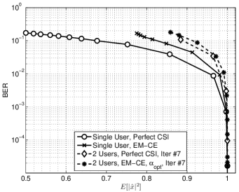
Figure 2: BER vs. soft values in a 1 user system (solid lines) and 2 user system (dashed lines) with 2 dB power imbalance.

IV Simulation Study

A simulation study was carried out in order to evaluate the performance of the proposed partial interference cancellation scheme. A simulation setting with two symbol and frame asynchronous users is used. The channel code is the UMTS turbo code [12]. The code rates of user $1$ and user $2$ are $0.72$ and $0.53$ respectively. The number of SIC stages is set to $7$ in all cases, as no meaningful performance improvement is observed after this point. In each stage each user performs $15$ iterations of the EM algorithm. Both transmitters employ the same random interleaver. The modulation used is BPSK for both users, and the code block length is $C_{u}=5000$ symbols, $\forall u$. The number of pilot symbols per code block is $X_{u,p}=256,\forall u$. Pilot symbols are boosted by $3$ dB with respect to data symbols. The channel is assumed to be AWGN and the phase noise increase between two consecutive symbols has a variance $\sigma_{p}^{2}=100/f_{0}$ rad²/symbol, where $f_{0}$ is the baud rate (in our simulations 10 kBaud). Different simulations were carried out for power imbalance, $P_{U,u_{1},u_{2}}$, ranging from $1$ dB to $7$ dB, being user $1$ always the strongest one. In contrast to much of the work on MUD, no spreading is employed.

Our scheme is compared to multistage full SIC with EM based CE (very akin to [7]). Fig. 3 and Fig. 4 show the BER of user $1$ and $2$, respectively, for a power imbalance of $2$ dB. If we analyze the SNR at which the different schemes reach a BER of $1e-4$, for both users optimal partial SIC results in a SNR gain of $2$ dB with respect to full SIC. Moreover, we can see how optimal partial SIC with $2$ stages outperforms full SIC with $7$ stages. However, both SIC schemes with estimated CSI are far from the performance achieved by perfect CSI. For optimal partial CSI the loss with respect to perfect CSI is $2$ dB for both users, half of the gap of the state-of-the art system.

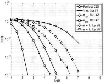
Figure 3: BER vs. SNR for the first user, power imbalance $2$ dB.

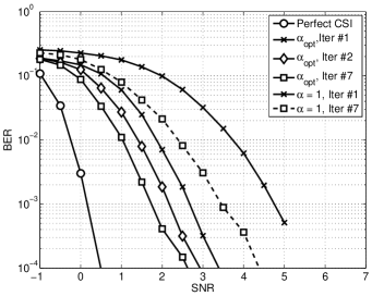
Figure 4: BER vs. SNR for the second user, power imbalance $2$ dB.

Fig. 5 shows the evolution of $\bar{E}$ with the SNR for user $2$. It can be seen how after $7$ SIC stages the scheme with optimal partial SIC outperforms full SIC. However the performance of both schemes is far from the performance of the single user case. The reason for this is the remaining interference from user $1$. It is also quite remarkable that optimal partial SIC after $2$ stages outperforms again full SIC with $7$ stages. Another important fact is that there is a floor at $\bar{E}=0.031$, which is caused by the presence of strong phase noise. Such problem clearly limits the performance of SIC since the interference can never be completely canceled. The evolution of $\bar{E}$ for user $1$, which is not shown in any figure, is very similar to that of user $2$, presenting also the same floor.

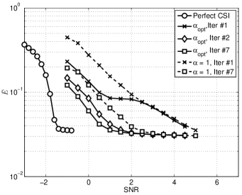
Figure 5: Normalized mean square error in the channel estimate $\bar{E}$ for the second user with a 2 dB power imbalance between the two users.

The evolution of $\alpha_{u}^{(d)}$ with respect to the SNR is shown in Fig. 6. It can be seen how $\alpha_{u}^{(d)}$ increases with the number of SIC stages. The figure also shows how the maximum value of $\alpha_{u}^{(d)}$ is $0.97<1$. The maximum possible value (i.e., 1) is not reacheable because of the presence of a floor in the channel estimation. The proposed scheme is aware of this floor and avoids full removal of the estimated signal.

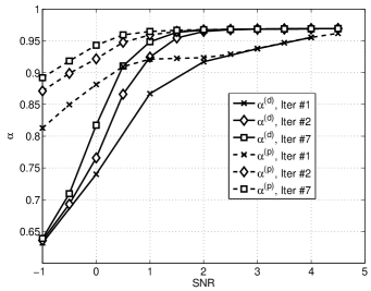
Figure 6: Evolution of the $\alpha$ factor for the second user as a function of the SNR. The power imbalance is 2 dB.

Finally, Fig. 7 shows the SNR at which optimal partial SIC and full SIC reach BER $1e-4$ for different power imbalances. It can be seen how the gain provided by optimal partial SIC is high for low power imbalance and decreases as the power imbalance increases. Note that in many cases the optimal choice of $\alpha$ halves the gap to perfect CSI given this time varying channel.

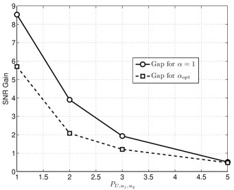
Figure 7: Additional SNR required by the MUD schemes with respect to perfect CSI as a function of the power imbalance.

V Conclusions

The principle of soft SIC hinges on the idea that a low confidence on the decoded bits would reduce the amount of subtracted interference. The EM algorithm is known to be an effective tool to improve the performance of MUD. However, it has the side effect of leading to overconfidence in the LLRs which has a negative effect on the performance of SIC. The optimal weighting factor $\alpha$ for SIC has been derived, which is able to partially compensate for this overconfidence in the LLRs. Moreover, it is also able to mitigate the negative impact of imperfect CSI. The proposed technique shows gains up to 3 dB when the detected users are received with comparable powers. Furthermore, the performance gap between perfect CSI and the state of the art is roughly halved by the suggested scheme.

VI Acknowledgments

The authors would like to acknowledge Dr. G. Liva and G. Garramone for the useful discussions.

The authors are supported inpart by the Space Agency of the German Aerospace Center and the Federal Ministry of Economics and Technology based on the agreement of the German Bundestag with the support code 50 YB 0905 and in part by the ESA Contract No. 23030/10/NL/CLP ”NICOLE”.

References

- [1] S. Verdú, Multiuser Detection. Cambridge (UK): Cambridge University Press, 1998.
- [2] J. Hou, J. E. Smee, H. D. Pfister, and S. Tomasin, “Implementing interference cancellation to increase the EV-DO Rev A reverse link capacity,” IEEE Commun. Mag., vol. 44, no. 2, p. 58 64, Feb. 2006.
- [3] J. Andrews, “Interference cancellation for cellular systems: A contemporary overview,” IEEE Wireless Commun. Mag., no. 4, pp. 19–29, Apr. 2005.
- [4] “Special issue on multiuser detection for advanced communication systems and networks,” IEEE J. Select. Areas Commun., vol. 26, no. 3, Apr. 2008.
- [5] X. Wang and V. H. Poor, Wireless Communications Systems: Advanced Techniques for Signal Reception. Prentice Hall, 2003.
- [6] M. Valenti and B. Woerner, “Iterative channel estimation and decoding of pilot symbol assisted turbo codes over flat-fading channels,” Selected Areas in Communications, IEEE Journal on, vol. 19, no. 9, pp. 1697 –1705, sep 2001.
- [7] M. Kobayashi, J. Boutros, and G. Caire, “Successive Interference Cancellation With SISO Decoding and EM Channel Estimation,” IEEE J. Select. Areas Commun., vol. 19, no. 8, pp. 1450–1460, Aug. 2001.
- [8] J. Wehinger and C. F. Mecklenbräuker, “Iterative CDMA Multiuser Receiver With Soft Decision-Directed Channel Estimation,” IEEE Trans. Signal Processing, vol. 54, no. 10, pp. 3922–3934, Oct. 2006.
- [9] L. Hageman and D. Young, Applied Iterative Methods. Mineola (NY, USA): Dover Publishing, 2004.
- [10] R. Nambiar and A. Goldsmith, “Iterative weighted interference cancellation for CDMA systems with RAKE reception,” in IEEE VTC Spring, Houston (TX, USA), May 1999.
- [11] D. Divsalar, M. K. Simon, and D. Raphaeli, “Improved Parallel Interference Cancellation for CDMA,” IEEE Trans. Commun., vol. 46, no. 2, pp. 258–268, Feb. 1998.
- [12] UMTS Multiplexing and Channel Coding (FDD), ETSI TS 25.212 v9.2, 3GPP Std., March 2010.
- [13] W. E. Ryan and S.Lin, Channel Codes – Classical and Modern. Cambridge University Press, 2009.
- [14] G. Colavolpe, A. Barbieri, and G. Caire, “Algorithms for iterative decoding in the presence of strong phase noise,” IEEE J. Select. Areas Commun., vol. 23, no. 9, pp. 1748–1757, Sept. 2005.
- [15] J. Boutros and G. Caire, “Iterative multiuser joint decoding: unified framework and asymptotic analysis,” Information Theory, IEEE Transactions on, vol. 48, no. 7, pp. 1772 –1793, July 2002.
- [16] L. Rasmussen, A. Grant, and P. Alexander, “An extrinsic kalman filter for iterative multiuser decoding,” Information Theory, IEEE Transactions on, vol. 50, no. 4, pp. 642 – 648, 2004.
- [17] A. P. Dempster, N. M. Laird, and D. B. Rubin, “Maximum-likelihood from incomplete data via the EM algorithm,” J. Roy. Stat. Soc., vol. 39, no. 1, pp. 1 –38, January 1977.
- [18] J. Boutros, “A tutorial on iterative probabilistic decoding and channel estimation,” in IAP MOTION, Ghent (Belgium), Jan. 2005.
- [19] C. Herzet, N. Noels, V. Lottici, H. Wymeersch, M. Luise, M. Moeneclaey, and L. Vandendorpe, “Code-aided turbo synchronization,” Proc. IEEE, vol. 95, no. 6, pp. 1255 –1271, June 2007.
- [20] D. Tse and P. Viswanath, Fundamentals of Wireless Communication. Cambridge Univ. Press, 2008.
- [21] S. Haykin, M. Sellathurai, Y. de Jong, and T. Willink, “Turbo-MIMO for wireless communications,” IEEE Commun. Mag., no. 10, pp. 48–53, Oct. 2004.
- [22] S. Sambhwani, W. Zhang, and W. Zeng, “Uplink Interference Cancellation in HSPA: Principles and Practice,” 2009.