On the Spatial Degrees of Freedom of Multicell and Multiuser MIMO Channels

Abstract

We study the converse and achievability for the degrees of freedom of the multicellular multiple-input multiple-output (MIMO) multiple access channel (MAC) with constant channel coefficients. We assume $L>1$ homogeneous cells with $K\geq 1$ users per cell where the users have $M$ antennas and the base stations are equipped with $N$ antennas. The degrees of freedom outer bound for this $L$-cell and $K$-user MIMO MAC is formulated. The characterized outer bound uses insight from a limit on the total degrees of freedom for the $L$-cell heterogeneous MIMO network. We also show through an example that a scheme selecting a transmitter and performing partial message sharing outperforms a multiple distributed transmission strategy in terms of the total degrees of freedom. Simple linear schemes attaining the outer bound (i.e., those achieving the optimal degrees of freedom) are explores for a few cases. The conditions for the required spatial dimensions attaining the optimal degrees of freedom are characterized in terms of $K$, $L$, and the number of transmit streams. The optimal degrees of freedom for the two-cell MIMO MAC are examined by using transmit zero forcing and null space interference alignment and subsequently, simple receive zero forcing is shown to provide the optimal degrees of freedom for $L>1$. By the uplink and downlink duality, the degrees of freedom results in this paper are also applicable to the downlink. In the downlink scenario, we study the degrees of freedom of $L$-cell MIMO interference channel exploring multiuser diversity. Strong convergence modes of the instantaneous degrees of freedom as the number of users increases are characterized.

I Introduction

Over the past few years, a significant amount of research has gone into making various techniques for enhancing spectrum reusability reality. Spatial techniques such as multiple-input multiple-output (MIMO) wireless systems have been widely studied to improve the spectrum reusability. Recently, the scope of spatial transmission has been extended to MIMO network wireless systems such as the interference network, relay network, and multicellular network. Network MIMO systems are now an emphasis of IMT-Advanced and beyond systems. In these networks, out-of-cell (or cross cell) interference is a major drawback. Before network MIMO can be deployed and used to its full potential, there are a large number of challenging issues. Many of these deal with interference management and joint processing between nodes to suppress out-of-cell interference (e.g., see the references in [1]).

I-A Overview

Understanding the information-theoretic capacity of general network MIMO is still challenging even under full cooperation assumptions. Alternatively, there are various approaches to approximate the capacity in the high SNR regime (some of which can be practically achieved in small cell scenarios [1]) by analyzing the number of resolvable interference-free signal dimensions in terms of the degrees of freedoms of the network. Initial works include the degrees of freedom and/or capacity region characterization for the MIMO multiple access channel (MAC) [2] and MIMO broadcast channel [3, 4, 5, 6]. While the general capacity region of the interference channel is not known, there are some known capacity results with very strong [7] and strong [8, 9] interference. The capacity outer bounds [10, 11] and degrees of freedom outer bounds [12, 13] for the multiple nodes interference channel with single antenna nodes have been characterized. Recently, the degrees of freedom have been studied for the two node MIMO X channel [14, 15] and the two user MIMO interference channel [16]. The key innovation used to prove the inner bound on the degrees of freedom is interference alignment [15, 16].

Interference alignment aims to allow coordinated transmission and reception in order to increase the total degrees of freedom of the network. Interference alignment generates overlapping user signal spaces occupied by undesired interference while keeping the desired signal spaces distinct. When an achievable scheme achieves the degrees of freedom of the converse, we say that the scheme attains the optimal degrees of freedom.

The fundamental idea of interference alignment in [15, 16] is extended to the multiple node X channel in [17], $K$-user interference channel in [18, 19], and more general cellular networks in [20] under a time or frequency varying channel assumption. For the X channel with single antenna users, interference alignment achieves the optimal degrees of freedom for the $K$ by $L\!=\!2$ (or $K\!=\!2$ by $L$) X channel with finite symbol extension, but for $K>2$ and $L>2$, it requires infinite symbol extension [17]. The $K$-user interference channel with single antenna nodes [18] and multiple antenna nodes [19] also needs infinite symbol extension.Various aspects of interference alignment for cellular networks are investigated in [20] including the effect of a multi-path channel and channel with propagation delay. The work in [20] shows that a single degree of freedom can be achieved per user as the number of users grows large with symbol extension.

In the case of constant channel coefficients, the spatial degrees of freedom have mainly been investigated. For the two by two MIMO X channel, the exact optimal degrees of freedom of $\frac{4}{3}M$ is achievable when each node has $M>1$ antennas [15, 14]. The optimal degrees of freedom of the two user MIMO interference channel is shown to be $\min\left(2M,2N,\max(M,N)\right)$ in [16], where $M$ and $N$ denote the number antennas at the transmitter and receiver, respectively. Remarkably, simple zero forcing is sufficient to provide the optimal degrees of freedom [15, 16]. Interference alignment in a three-user interference channel with $M=N$ antennas at each node yields the optimal degrees of freedom of $\frac{3M}{2}$ when $M$ is even (when $M$ is odd a two symbol extension is required to achieve $\frac{3M}{2}$) [18]. Compared to the prototypical examples of the two-user MIMO interference channel or two by two MIMO X channel, the general characterization of the optimal degrees of freedom for the multicell multiuser MIMO networks (that works for an arbitrary numbers of users and cells) with constant channel coefficients is still an open problem. When studying the achievable scheme with constants channel coefficients, the number of required $M$ and $N$ must be determined as a function of the number of cells ($L$) and users ($K$) or vice versa. Thus, taking into consideration all of these dependencies often makes the characterization overconstrained. Recently, an achievable scheme where each user obtains one degree of freedom for the two cell and $K$-user MIMO network with constant channel coefficients is proposed for $N=M=K+1$ in [21]. In an $L$-cell and $K$-user MIMO network, a necessary zero interference condition on $M$ and $N$ (as a function of $K$ and $L$) to provide one interference free dimension to each of users is investigated in [22].

The conventional interference alignments and other linear schemes in [15, 16, 17, 18, 19, 20] require global notion of CSI at all nodes, and the optimal degrees of freedom is particularly attained by extending signals over large space/time/frequency dimensions. To overcome these challenges, efficient interference alignment schemes that only utilize local CSI feedback are considered in [23, 21]. An efficient way to provide additional degrees of freedom gain without a global notion of CSI and, at the same time, with a reduced amount of feedback is to exploit multiuser diversity as in [24, 25]. The basic notion of the multiuser diversity with multiple antennas in [24, 25] has been recently extended to interference networks, namely through opportunistic interference alignment, such as for the case of a cognitive network [26], cellular uplink [27], and cellular downlink [28, 29, 30]. The common idea is to schedule users (or dimensions in [26]) so that the interference caused by the selected users to the other receivers are aligned or minimized with the aid of power allocation [26, 29] and opportunistic transmit or receive filter design [26, 27, 28, 30]. The performance of the multiuser diversity is evaluated or analyzed in terms of the average throughput [26, 28, 29] and average degrees of freedom [27, 30].

I-B Contributions

First, a simple characterization of the optimal degrees of freedom with constant channel coefficient for the multicell MIMO MAC is provided. Then, a scenario when the downlink system exploits the multiuser diversity is considered and the degrees of freedom by employing user scheduling is characterized.

In the uplink, we assume $L$ homogeneous cells with $K$ users per cell. We do not consider time or frequency domain extensions with a time or frequency varying channel assumption. Alternatively, spatial resources are utilized with constant channel coefficients. Although our focus is on the scenario where the transmitter and receiver have $M$ and $N$ antennas, we show a spatial degrees of freedom outer bound for the $L$-cell and $K$-user MIMO MAC that includes the case when each node has a different number of antennas. For the two-cell case, two linear schemes that achieve the degrees of freedom outer bound are characterized. The first scheme is a simple transmit zero forcing with $M=K\beta+\beta$ and $N=K\beta$, and the second one is a null space interference alignment with $M=K\beta$ and $N=K\beta+\beta$, where $\beta>0$ is a positive integer. For $L>1$ (including the two-cell case), it is verified that receive zero forcing with $M=\beta$ and $N=KL\beta$ precisely achieves the optimal degrees of freedom for $K\geq 1$.

The main ingredients of the degrees of freedom outer bound, analogous to [12, 17, 18, 19], are to split whole messages into small subsets so that the outer bound can tractably be formulated for each of message subsets. We define the message subset for the $L$-cell heterogeneous networks where $L-1$ cells form an $L-1$-user MIMO interference channel and a single cell forms a $K$-user MIMO MAC. We also investigate through an example that selecting a subset of transmitters and allowing them to use partial message sharing (through perfect links) achieves a higher degrees of freedom than distributed MIMO transmission.

Null space interference alignment for the two-cell case is developed for the uplink scenario with $N>M$ to show the achievability of the converse. It relies on each base station using a carefully chosen null space plane. The null space planes are designed to project the out-of-cell interference to a lower dimensional subspace than its original dimension so that the null space plane can jointly mitigate the degrees of freedom loss coming from the out-of-cell interference. The dimensions of the interference free signal at each base station after projection depend on the “size” of the overlapped out-of-cell interference null space, which is referred to as the geometric multiplicity of the out-of-cell interference null space (the definition will be clearer in Section V). We generalize the null space interference alignment framework for various kinds of antenna dimensions. Though it does not necessarily achieve the optimal degrees of freedom, it resolves $\beta>0$ interference free dimensions per user. Notice that by the uplink and downlink duality the degrees of freedom results obtained for the uplink are also applicable to the downlink.

Next, we study the degrees of freedom of the $L$-cell downlink interference channel by exploiting multiuser diversity. One of the key aspects for the interference alignment in [17, 18, 19, 20] is in its almost sure (a.s.) convergence argument on the instantaneous degrees of freedom with infinite symbol extension across time and frequency. In line with the convergence argument made in interference alignments, we show that this strong convergence argument on the instantaneous degrees of freedom still holds when utilizing many users in the network. We quantify the additional degrees of freedom achievable through the user scheduling where the user scheduling only uses the local CSI. This exhibits clear comparison on the instantaneous degrees of freedom between the multiuser diversity system and interference alignment in [17, 18, 19, 20]. We show in particular that if the number of candidate users that participate in scheduling in a cell increases faster than linearly with SNR, the instantaneous degrees of freedom converges to $L$ in both mean-square (m.s.) sense and almost sure (a.s.) sense for the $L$-cell downlink MIMO interference channel with $M=1$ and $N=L-1$.

The rest of the paper is outlined as follows. Section II describes the system model. In Section III, the degrees of freedom outer bound for $L$-cell and $K$-user MIMO MAC is formulated. The conditions for the optimal degrees of freedom are characterized in Section IV. In Section V, general frameworks for the null space interference alignment for various kinds of spatial dimension conditions are investigated. Section VI discusses the instantaneous degrees of freedom with multiuser diversity for the $L$-cell downlink MIMO interference channel. The paper is concluded in Section VII.

II System Model

We first define the uplink channel model. The downlink channel model is simply described by the uplink and downlink duality.

II-A Uplink Channel Model

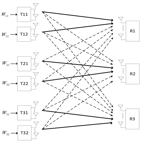
Figure 1: Multicell MIMO MAC with $L=3$ and $K=2$.

Consider a network that consists of $L$ homogeneous cells. In each cell, there are $K\geq 1$ users and one base station, where each user has $M\geq 1$ antennas and the base station is equipped with $N\geq 1$ antennas. We introduce an index $\ell k$ to correspond to user $k$ in cell $\ell$ for $\ell\in{\mathcal{L}}$ and $k\in{\mathcal{K}}$ where ${\mathcal{L}}=\{1,\ldots,L\}$ and ${\mathcal{K}}=\{1,\ldots,K\}$, respectively. For instance, a $3$-cell MIMO MAC is shown in Fig. 1 where each cell consists of $2$ users (i.e., $L=3$ and $K=2$). Note that though our focus, in this paper, is on $L$ homogeneous cells where the transmitter and receiver have $M$ and $N$ antennas, respectively, we generalize the degrees of freedom outer bound when user $\ell k$ has $M_{\ell k}$ antenna and base station $\ell$ has $N_{\ell}$ antennas in Section III-A.

The channel input-output relation at the $t$th discrete time slot is described as

$${\mathbf{y}}_{m}(t)=\sum_{\ell=1}^{L}\sum_{k=1}^{K}{\mathbf{H}}_{m,\ell k}{\mathbf{x}}_{\ell k}(t)+{\mathbf{z}}_{m}(t),\ m\in{\mathcal{L}}$$ (1)

where ${\mathbf{y}}_{m}(t)\in{\mathbb{C}}^{N\times 1}$ and ${\mathbf{z}}_{m}(t)\in{\mathbb{C}}^{N\times 1}$ denote the received signal vector and additive noise vector at the base station $m$, respectively. Each entry of ${\mathbf{z}}_{m}(t)$ is independent and identically distributed (i.i.d.) with ${\mathcal{C}}{\mathcal{N}}(0,1)$. The vector ${\mathbf{x}}_{\ell k}(t)\in{\mathbb{C}}^{M\times 1}$ in (1) represents the user $\ell k$’s transmit vector at $t$th channel use. The channel input is subject to an individual power constraint

$$E\left[\left\|{\mathbf{x}}_{\ell k}(t)\right\|^{2}\right]=\mathop{\mathrm{tr}}\left(E\left[{\mathbf{x}}_{\ell k}(t){\mathbf{x}}_{\ell k}^{*}(t)\right]\right)\leq\rho,\ k\in{\mathcal{K}},\ell\in{\mathcal{L}}$$ (2)

where $\rho$ represents SNR. The matrix ${\mathbf{H}}_{m,\ell k}\in{\mathbb{C}}^{N\times M}$ in (1) denotes the channel with constant coefficients from user $\ell k$ to base station $m$. Moreover, $\left\{{\mathbf{H}}_{m,mk}\right\}_{k\in{\mathcal{K}}}$ represent the desired data channels at base station $m$ while the matrices $\left\{{\mathbf{H}}_{m,\ell k}\right\}_{\ell\in{\mathcal{L}}\backslash m,k\in{\mathcal{K}}}$ carry out-of-cell interference to base station $m$. All the channel matrices are sampled from continuous distributions, and each entry of ${\mathbf{H}}_{m,\ell k}$ is i.i.d. (i.e., we basically assume a rich scattering environment). This channel model almost surely ensures all channel matrices have full rank, i.e., $\mathop{\mathrm{rank}}({\mathbf{H}}_{m,\ell k})=\min(M,N)$ for $m,\ell\in{\mathcal{L}}$ and $k\in{\mathcal{K}}$. The channel gains from different users are mutually independent. This channel condition where all channel matrices with i.i.d. are full rank is referred to as nondegenerate in this paper.

Define $W_{\ell k}(\rho)$ as a message from user $\ell k$ to the destined base station $\ell$ at SNR $\rho$. The message $W_{\ell k}(\rho)$ is uniformly distributed in a $(n,2^{nR_{\ell k}(\rho)})$ codebook ${\mathcal{Z}}(\rho)$$=$$\{\zeta_{1}(\rho),\ldots,\zeta_{2^{nR_{\ell k}(\rho)}}(\rho)\}$, and messages at different users are independent of each other. In order to approach the capacity, the data rate of the coding scheme increases with respect to (w.r.t) $\rho$. This includes a coding scheme where the codebook is chosen from a sequence of codebooks $\left\{{\mathcal{W}}(\rho)\right\}$ for each level of $\rho$. The message $W_{\ell k}(\rho)$ is mapped to ${\mathbf{x}}_{\ell k}(t)$ in (1) over $n$ channel uses. Then, the information transfer rate $R_{\ell k}(\rho)$ of message $W_{\ell k}(\rho)$ is said to be achievable if the probability of decoding error can be made arbitrarily small by choosing an appropriate channel block length $n$. The capacity region ${\mathcal{C}}(\rho)$ is the set of all achievable rate tuples $\{R_{\ell k}(\rho)\}_{\ell\in{\mathcal{L}},k\in{\mathcal{K}}}$.

II-B Degrees of Freedom

We define the spatial degrees of freedom of the multicell MIMO MAC as

$$\mathbf{\Sigma}_{d}=\lim_{\rho\rightarrow\infty}\sum_{\{R_{\ell k}(\rho)\}_{\ell\in{\mathcal{L}},k\in{\mathcal{K}}}\in{\mathcal{C}}(\rho)}\frac{R_{\ell k}(\rho)}{\log(\rho)}.$$ (3)

A network has $\mathbf{\Sigma}_{d}$ degrees of freedom if the sum capacity is expressed as $\mathbf{\Sigma}_{d}\log(\rho)\!+\!o(\log(\rho))$. This implies that the degrees of freedom $\mathbf{\Sigma}_{d}$ is equivalent to the total number of interference free signal dimensions (i.e., the number of effective single-input single-output (SISO) data streams that can be supported).

The degrees of freedom measure $\mathbf{\Sigma}_{d}$ in (3) ignores any fixed (or vanishing) quantities in the achievable sum rate expression as $\rho$ increases. Notice that the quantity $\mathbf{\Sigma}_{d}$ in (3) is characterized as a convergence of random variables $\left\{\frac{R_{\ell k}(\rho)}{\log(\rho)}\right\}_{\ell\in{\mathcal{L}},k\in{\mathcal{K}}}$ as $\rho\rightarrow\infty$. The degrees of freedom results in [15, 16, 17, 18, 19, 20] show this convergence as almost sure (a.s.) sense. When we refer the degrees of freedom in Section III, IV, and V, that implies $\mathbf{\Sigma}_{d}$ characterized with instantaneous achievable rates $\{R_{\ell k}(\rho)\}_{\ell\in{\mathcal{L}},k\in{\mathcal{K}}}$. While, when we explore the multiuser diversity in Section VI, we need to distinguish between the instantaneous degrees of freedom and the average degrees of freedom in order to capture the detailed difference in user scaling laws. Notice that the former includes the mode of the convergence in random sequences $\left\{\frac{R_{\ell k}(\rho)}{\log(\rho)}\right\}_{\ell\in{\mathcal{L}},k\in{\mathcal{K}}}$ as $\rho,K\rightarrow\infty$, while the later does not include detailed convergence argument.

In what follows, we will omit the $\rho$ attached to $W_{\ell k}(\rho)$ and $R_{\ell k}(\rho)$. In addition, with an abuse of notation, ${\mathbf{y}}_{m}(t)$, ${\mathbf{z}}_{m}(t)$, and ${\mathbf{x}}_{\ell k}(t)$ in (1) are simplified to ${\mathbf{y}}_{m}$, ${\mathbf{z}}_{m}$, and ${\mathbf{x}}_{\ell k}$.

II-C Downlink Channel Model

The uplink scenario is converted to the downlink scenario by changing the role of the transmitter and receiver and defining the reciprocal channel for the downlink as shown in [23, 20, 22] (i.e., uplink and downlink duality). By $L$-cell and $K$-user MIMO downlink, we mean the network in which there are total $L$ transmitters and $K$ distributed receivers in each of cells. In the downlink, we use the index $k\ell$ to correspond to user $k$ in cell $\ell$ for $k\in{\mathcal{K}}$ and $\ell\in{\mathcal{L}}$.

The received vector at user $k$ in cell $m$ is expressed by

$${\mathbf{y}}_{km}=\sum_{\ell=1}^{L}{\mathbf{H}}_{km,\ell}{\mathbf{x}}_{\ell}+{\mathbf{n}}_{km}$$ (4)

where ${\mathbf{y}}_{km}$ and ${\mathbf{n}}_{km}$ are the $N\times 1$ received vector and additive white Gaussian noise vector (distributed as ${\mathcal{C}}{\mathcal{N}}(\mathbf{0},{\mathbf{I}}_{N})$), respectively, at user $km$. In (4), ${\mathbf{H}}_{km,\ell}\in{\mathbb{C}}^{N\times M}$ denotes the channel matrix from transmitter $\ell$ to user $km$. The nondegenerate channel condition, channel input power constraint, and encoding scheme are similarly defined as in uplink channel model. We will use this downlink model in Section VI to investigate the degrees of freedom with multiuser diversity.

III Degrees of Freedom Outer Bound of the $L$-cell and $K$-user MIMO MAC

III-A Degrees of Freedom Outer Bound

Given the channel model in (1), we now formulate the degrees of freedom outer bound for the $L$-cell and $K$-user MIMO MAC when transmitter $\ell k$ has $M_{\ell k}$ antennas and receiver $\ell$ has $N_{\ell}$ antennas. The following is the main result of this section.

Theorem 1

The total degrees of freedom of the $L$-cell and $K$-user MIMO MAC with $L>1$ and $K\geq 1$, whose channel matrices are nondegenerate, is bounded by

$$\mathbf{\Sigma}_{d}\leq\min\left(\sum_{\ell\in{\mathcal{L}},k\in{\mathcal{K}}}M_{\ell k},\sum\limits_{\ell\in{\mathcal{L}}}N_{\ell},\eta({\mathcal{W}})\right)$$ (5)

where

$$\eta({\mathcal{W}})=\frac{\sum\limits_{\ell\in{\mathcal{L}},k\in{\mathcal{K}}}\min\left(\sum\limits_{q\in{\mathcal{K}}}M_{\ell q}\!+\!\sum\limits_{p\in{\mathcal{L}}\backslash\ell}M_{pk},\sum\limits_{p\in{\mathcal{L}}}N_{p},\max\left(\sum\limits_{q\in{\mathcal{K}}}M_{\ell q},\sum\limits_{p\in{\mathcal{L}}\backslash\ell}N_{p}\right),\max\left(\sum\limits_{p\in{\mathcal{L}}\backslash\ell}M_{pk},N_{\ell}\right)\right)}{K+L-1}$$ (6)

with ${\mathcal{L}}=\left\{1,\ldots,L\right\}$, ${\mathcal{K}}=\left\{1,\ldots,K\right\}$, and ${\mathcal{W}}=\left\{W_{\ell k}\right\}_{\ell\in{\mathcal{L}},k\in{\mathcal{K}}}$.

Proof:

The approach taken to derive the outer bound in (5) is to split the whole message set ${\mathcal{W}}=\left\{W_{\ell k}\right\}_{\ell\in{\mathcal{L}},k\in{\mathcal{K}}}$ into subsets, derive the outer bound associated with each of the subsets, and combine all of the outer bounds to gain the total degrees of freedom outer bound. In addition, we assume perfect channel knowledge of all links at all nodes.

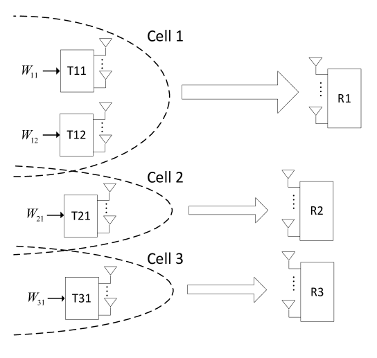
Figure 2: $(1,2)$ MAC-IC uplink HetNet consisting of a $2$-user MIMO MAC (i.e., cell $1$) and $2$-user MIMO interference channel (i.e., cell $2$ and $3$).

Suppose we reduce the $L$-cell and $K$-user MIMO MAC to an $L$-cell heterogenous MIMO uplink channel where the $L-1$ cells (among $L$ cells) constitute a $(L-1)$-user MIMO interference channel (IC) and the remaining single cell forms a $K$-user MIMO MAC. We refer to this network as the $(1,L-1)$ MAC-IC uplink HetNet. Fig. 2 represents the $(1,2)$ MAC-IC uplink HetNet composed of a single cell $2$-user MIMO MAC and $2$-user MIMO interference channel. This $(1,L-1)$ MAC-IC uplink HetNet is formed from the $L$-cell and $K$-user MIMO MAC by eliminating messages in ${\mathcal{W}}$ that do not constitute the information flow in the $(1,L-1)$ MAC-IC uplink HetNet channel.

Let the $\ell$th cell among $L$ cells is designated as the $K$-user MIMO MAC. Then, the rest of the $L-1$ cells forms an $(L-1)$-user MIMO interference channel by picking the $k$th user in each of the cells in ${\mathcal{L}}\backslash\ell$, i.e., the index set for the $L-1$ users is $\left\{1k,\ldots,(\ell-1)\ k,(\ell+1)\ k,\ldots Lk\right\}$. Message sets associated with the $K$-user MIMO MAC and $(L-1)$-user MIMO interference channel are then given by $\left\{W_{\ell q}\right\}_{q\in{\mathcal{K}}}$ and $\left\{W_{pk}\right\}_{p\in{\mathcal{L}}\backslash\ell}$, respectively. We define these two disjoint message sets as

$${\mathcal{W}}^{\ell k}=\left\{W_{\ell q}\right\}_{q\in{\mathcal{K}}}\cup\left\{W_{pk}\right\}_{p\in{\mathcal{L}}\backslash\ell}.$$ (7)

The degrees of freedom outer bound is first argued for each of the $LK$ sets $\left\{{\mathcal{W}}^{\ell k}\right\}_{\ell\in{\mathcal{L}},k\in{\mathcal{K}}}$, and $LK$ outer bounds are combined by accounting the overlapped messages.

Assume perfect cooperations between $K$ users in cell $\ell$ and between $L-1$ users and the corresponding $L-1$ receivers in the $(L-1)$-user MIMO interference channel. Then, the $(1,L-1)$ MAC-IC uplink HetNet with ${\mathcal{W}}^{\ell k}$ becomes a two-user interference channel with transmit and receive antenna pairs $\left(\sum\limits_{q\in{\mathcal{K}}}M_{\ell q},N_{\ell}\right)$ for the first link and $\left(\sum\limits_{p\in{\mathcal{L}}\backslash\ell}M_{pk},\sum\limits_{p\in{\mathcal{L}}\backslash\ell}N_{p}\right)$ for the second link. It is well known that the spatial degrees of freedom of an $(M_{1},N_{1})$, $(M_{2},N_{2})$ two-user MIMO interference channel is characterized as $\min(M_{1}+M_{2},N_{1}+N_{2},\max(M_{1},N_{2}),\max(M_{2},N_{1}))$ [15]. Thus, the degrees of freedom outer bound associated with message set ${\mathcal{W}}^{\ell k}$ is characterized by

$$\min\left(\sum\limits_{q\in{\mathcal{K}}}M_{\ell q}\!+\!\sum\limits_{p\in{\mathcal{L}}\backslash\ell}M_{pk},\sum\limits_{p\in{\mathcal{L}}}N_{p},\max\left(\sum\limits_{q\in{\mathcal{K}}}M_{\ell q},\sum\limits_{p\in{\mathcal{L}}\backslash\ell}N_{p}\right),\max\left(\sum\limits_{p\in{\mathcal{L}}\backslash\ell}M_{pk},N_{\ell}\right)\right).$$ (8)

In the same manner, the outer bound associated with the message set ${\mathcal{W}}^{\bar{\ell}\bar{k}}$ with $\bar{\ell}\neq\ell$ or $\bar{k}\neq k$ is also determined by (8). Since there are total $KL$ message subsets and each message repeats $K+L-1$ times over $KL$ message subsets (following from the splitting approach in (7)), from (8) the total degrees of freedom associated with ${\mathcal{W}}$ is bounded by

$$\mathbf{\Sigma}_{d}\leq\frac{\sum\limits_{\ell\in{\mathcal{L}},k\in{\mathcal{K}}}\min\left(\sum\limits_{q\in{\mathcal{K}}}M_{\ell q}\!+\!\sum\limits_{p\in{\mathcal{L}}\backslash\ell}M_{pk},\sum\limits_{p\in{\mathcal{L}}}N_{p},\max\left(\sum\limits_{q\in{\mathcal{K}}}M_{\ell q},\sum\limits_{p\in{\mathcal{L}}\backslash\ell}N_{p}\right),\max\left(\sum\limits_{p\in{\mathcal{L}}\backslash\ell}M_{pk},N_{\ell}\right)\right)}{K+L-1}.$$ (9)

Meanwhile, a trivial bound is obtained by allowing perfect cooperation among $KL$ transmitters and full cooperation corresponding $L$ receivers of the $L$-cell and $K$-user MIMO MAC as

$$\mathbf{\Sigma}_{d}\leq\min\left(\sum_{\ell\in{\mathcal{L}},k\in{\mathcal{K}}}M_{\ell k},\sum\limits_{\ell\in{\mathcal{L}}}N_{\ell}\right).$$ (10)

Combining two bounds in (9) and (10) yields the outer bound result in (5). ∎

The characterized bound is general, in that it includes networks with $K\geq 1$ and $L>1$ for arbitrary numbers of transmit and receive antennas.

The converse result in (5) can be further relaxed and simplified by upper bounding $\eta({\mathcal{W}})$ in (6) as

$$\eta({\mathcal{W}})\leq\min\!\left(\!\sum_{\ell\in{\mathcal{L}},k\in{\mathcal{K}}}\!\!M_{\ell k},\frac{KL\cdot\sum\limits_{p\in{\mathcal{L}}}\!N_{p}}{K+L-1},\frac{\sum\limits_{\ell\in{\mathcal{L}},k\in{\mathcal{K}}}\!\min\!\left(\!\max\left(\sum\limits_{q\in{\mathcal{K}}}M_{\ell q},\sum\limits_{p\in{\mathcal{L}}\backslash\ell}N_{p}\right),\max\left(\sum\limits_{p\in{\mathcal{L}}\backslash\ell}M_{pk},N_{\ell}\right)\!\right)}{K+L-1}\!\right)$$ (11)

where in (11) the summation $\sum\limits_{\ell\in{\mathcal{L}},k\in{\mathcal{K}}}$ is taken for operands inside of $\min(\cdot)$ in (6) and we use the facts that

$$\sum\limits_{\ell\in{\mathcal{L}},k\in{\mathcal{K}}}\frac{\sum\limits_{q\in{\mathcal{K}}}M_{\ell q}\!+\!\sum\limits_{p\in{\mathcal{L}}\backslash\ell}M_{pk}}{K+L-1}=\sum_{\ell\in{\mathcal{L}},k\in{\mathcal{K}}}M_{\ell k}$$

and

$$\sum\limits_{\ell\in{\mathcal{L}},k\in{\mathcal{K}}}\frac{\sum\limits_{p\in{\mathcal{L}}}N_{p}}{K+L-1}=\frac{KL\sum\limits_{p\in{\mathcal{L}}}N_{p}}{K+L-1}.$$

Since $\frac{KL}{K+L-1}\sum\limits_{p\in{\mathcal{L}}}N_{p}\geq\sum\limits_{\ell\in{\mathcal{L}}}N_{\ell}$ for $K,L\geq 1$, combining the two bounds in (11) and (10) yields

$$\mathbf{\Sigma}_{d}\leq\min\left(\sum_{\ell\in{\mathcal{L}},k\in{\mathcal{K}}}M_{\ell k},\sum\limits_{\ell\in{\mathcal{L}}}N_{\ell},\frac{\sum\limits_{\ell\in{\mathcal{L}},k\in{\mathcal{K}}}\min\left(\max\left(\sum\limits_{q\in{\mathcal{K}}}M_{\ell q},\sum\limits_{p\in{\mathcal{L}}\backslash\ell}N_{p}\right),\max\left(\sum\limits_{p\in{\mathcal{L}}\backslash\ell}M_{pk},N_{\ell}\right)\right)}{K+L-1}\right).$$ (12)

As mentioned earlier, our focus is mainly on an homogeneous antenna distribution. The next corollary presents the required outer bound.

Corollary 1

The total spatial degrees of freedom of the $L$-cell and $K$-user MIMO MAC with $M$ transmit antennas and $N$ receive antennas is bounded by

$$\mathbf{\Sigma}_{d}\leq\min\left(KLM,LN,\frac{KL}{K+L-1}\max\left(KM,(L-1)N\right),\frac{KL}{K+L-1}\max\left((L-1)M,N\right)\right).$$ (13)

Proof:

The bound can be obtained by substituting $M_{\ell k}=M_{\ell q}=M_{pk}=M$ and $N_{\ell}=N_{p}=N$ in (12) and taking all the summations. ∎

III-B $(1,L-1)$ MAC-IC Uplink HetNet

The characterized outer bound utilizes insight from a limit of the total degrees of freedom for an $L$-cell heterogeneous network, i.e., $(1,L-1)$ MAC-IC uplink HetNet. Denote $M_{q}$ and $N$ as the numbers of antennas at user $q$ and the base station in the $K$-user MIMO MAC, respectively, and represent $M_{p}$ and $N_{p}$ as the number antennas at user $p$ and the corresponding receiver in the $(L-1)$-user MIMO interference channel, respectively.

Corollary 2

Denote $\mathbf{\Sigma}_{L-1,1}$ as the total degrees of freedom of the $(L-1,1)$ MAC-IC uplink HetNet. Then,

$$\mathbf{\Sigma}_{L-1,1}\leq\min\left(\sum\limits_{q=1}^{K}M_{q}\!+\!\sum\limits_{p=1}^{L-1}M_{p},\sum\limits_{p=1}^{L}N_{p},\max\left(\sum\limits_{q=1}^{K}M_{q},\sum\limits_{p=1}^{L-1}N_{p}\right),\max\left(\sum\limits_{p=1}^{L-1}M_{p},N\right)\right)$$ (14)

Proof:

Omit $\ell$ and $k$ attached to $M_{\ell q}$, $N_{\ell}$, and $M_{pk}$ in (8). Then, the formula in (8) verifies the corollary. ∎

Interestingly, the collocated $(L-1)$-user MIMO interference channel and single cell $K$-user MIMO MAC can be viewed as a two-tier cell deployment where the network consists of $L-1$ femtocells (or picocells) each with a single user and one macrocell with $K$ users. Notice that in the two-tier networks, single user transmission at the lower-tier cell is shown to provide significantly improved throughput and coverage than multiuser transmission [31].

III-C Virtual MIMO Transmission vs. Selected and Shared Transmission

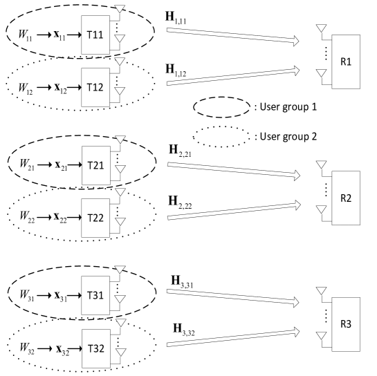
Figure 3: User grouping strategy for $L=3$ and $K=2$ MIMO MAC

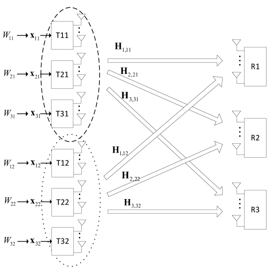
Figure 4: Conversion to distributed $2\times 3$ homogeneous MIMO X channel

Now we are interested in an equivalent channel model to the $L$-cell and $K$-user MIMO MAC. Consider groups of $L$ distinct users among the $LK$ users (i.e., a total of $K$ user groups) such that the $k$th user group is formed by grouping the $k$th user in each of the cells, i.e., the $k$th user group is the index set $\left\{1k,2k,\ldots,Lk\right\}$. For example, Fig. 3 shows the user grouping for the $L=3$ and $K=2$ MIMO MAC where the first user group is represented as the index set $\{11,21,31\}$, and the second user group consists of indices $\{12,22,32\}$. Then, the network is converted to a distributed $K\times L$ homogenous MIMO X channel (see Fig. 4). Here, the equivalent channel of the $L$-cell and $K$-user MIMO MAC is referred to as the distributed $K\times L$ homogenous MIMO X channel because perfect cooperation among users within each user group is not assumed.

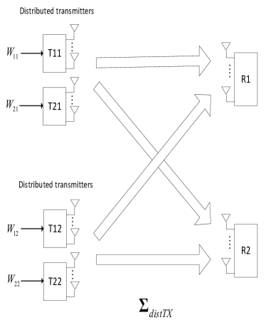
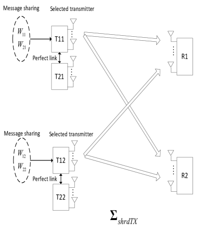
Figure 5: (a) Multiple distributed transmission ($L=2$ and $K=2$). (b) Selected and shared transmission through perfect links ($L=2$ and $K=2$)

The equivalency between the $L$-cell and $K$-user MIMO MAC and distributed $K\times L$ homogeneous MIMO X channel provides an interesting insight into the following question: When using spatial dimensions to transmit messages $\left\{W_{\ell k}\right\}_{\ell\in{\mathcal{L}},k\in{\mathcal{K}}}$, is it better to employ multiple distributed transmission where transmitter $\ell k$, equipped with $M$ antennas, transmits its own message $W_{\ell k}$ or to employ selected and shared transmission where one transmitter, say $1k$ in the $k$th user group $\left\{1k,2k,\ldots,Lk\right\}$, equipped with $M$ antennas, is selected and transmits all of the messages $\left\{W_{1k},W_{2k},\ldots,W_{Lk}\right\}$ while other transmitters in the group keep quiet? Given full CSI at all nodes, multiple distributed transmission delivers messages $\left\{W_{\ell k}\right\}_{\ell\in{\mathcal{L}},k\in{\mathcal{K}}}$ through distributed transmitters with the use of total $LKM$ dimensions (e.g., virtual MIMO transmission), while selected and shared transmission uses $KM$ dimensions with the use of partial message sharing through the perfect links between transmitters. We can show the later strategy is better in terms of the degrees of freedom than the former strategy for $L=2$ and $K=2$ (see Fig. 5 (a) and Fig. 5 (b)) as follows.

Corollary 3

Let $\mathbf{\Sigma}_{distTX}$ and $\mathbf{\Sigma}_{shrdTX}$ denote the total degrees of freedom of the multiple distributed transmission and selected and shared transmission, respectively, when $L=2$ and $K=2$ with $M=N$. Then,

$$\mathbf{\Sigma}_{distTX}\leq\mathbf{\Sigma}_{shrdTX}.$$

Proof:

Since the multiple distributed transmission with $L=2$ and $K=2$ in Fig. 5 (a) is equivalent to $2$-cell and $2$-user MIMO MAC, from Corollary 1

$$\mathbf{\Sigma}_{distTX}\!\!\!\! = \!\!\!\!\mathbf{\Sigma}_{d}$$

$$\leq \!\!\!\!\min\left(4M,2M,\frac{4}{3}\max(2M,M),\frac{4}{3}\max(M,M)\right)=\frac{4}{3}M.$$

The selected and shared transmission through perfect link with $L=2$ and $K=2$ is the $2\times 2$ MIMO X channel with $M$ antennas at each node. Hence,

$$\mathbf{\Sigma}_{shrdTX}=\frac{4}{3}M$$

where the last equality follows from the optimal degrees of freedom result in [16] where the achievable scheme utilizes the simple zero forcing. ∎

In what follows, we will quote the results in this section to characterize the optimal degrees of freedom for $L$-cell and $K$-user MIMO MAC.

IV Achieving the Optimal Degrees of Freedom

In the homogenous $L$-cell and $K$-user MIMO MAC, independently encoded $\beta>0$ streams are transmitted as ${\mathbf{x}}_{mk}={\mathbf{T}}_{mk}{\mathbf{s}}_{mk}$ from user $mk$ to base station $m$, where ${\mathbf{s}}_{mk}\!=\!\left[s_{mk,1}\ldots s_{mk,\beta}\right]^{T}$ is the $\beta\times 1$ symbol vector carrying message $W_{mk}$ and ${\mathbf{T}}_{mk}\in{\mathbb{C}}^{M\times\beta}$ denotes a linear precoder which will be chosen to provide interference free signal dimensions to user $mk$. The $N$-dimensional signal received at base station $m$ is expressed as

$${\mathbf{y}}_{m}\!=\!\sum_{k=1}^{K}\!{\mathbf{H}}_{m,mk}{\mathbf{T}}_{mk}{\mathbf{s}}_{mk}\!+\!\sum_{\ell\neq m}^{L}\sum_{k=1}^{K}{\mathbf{H}}_{m,\ell k}{\mathbf{T}}_{\ell k}{\mathbf{s}}_{\ell k}\!+\!{\mathbf{z}}_{m}.$$ (15)

The achievable schemes must deal with $K(L\!-\!1)\beta$ out-of-cell interference sources and additionally $(K\!-\!1)\beta$ inner cell interference sources. This implies that the required spatial antenna dimensions $M$ and $N$ for the zero interference condition with constant channel coefficients must be determined as a function of $K$, $L$, and $\beta$.

Our base line algorithm is to explore the feasibility of the linear schemes utilizing the spatial dimensions under zero interference constraints. Given (15), our base line algorithm utilizes linear postprocessing matrix ${\mathbf{P}}_{m}\in{\mathbb{C}}^{K\beta\times N}$ at receiver $m$ to produce $\beta$ interference free dimensions for each of users. The two-cell MIMO MAC scenario, which is instructive, is first considered, and a general multicell case is characterized later.

IV-A Two-Cell MIMO MAC ($L=2$)

The degrees of freedom outer bound in (13) and zero forcing-based linear schemes allow the following theorem to be proven.

Theorem 2

The two-cell and $K$-user MIMO MAC with the nondegenerate channels, where the transmitter and receiver have $M\!=\!K\beta$ and $N\!=\!K\beta\!+\!\beta$ or $M\!=\!K\beta\!+\!\beta$ and $N\!=\!K\beta$ antennas, respectively, has the optimal degrees of freedom of $2K\beta$ where $\beta>0$ is a positive integer.

Converse of Theorem 2

When $M=K\beta+\beta$ and $N=K\beta$, the outer bound in (13) returns

$$\mathbf{\Sigma}_{d}\!\!\!\! \leq \!\!\!\!\min\!\left(\!2KM,2N,\frac{2K\max(\!KM,N\!)}{K\!+\!1},\frac{2K\max(\!M,N\!)}{K\!+\!1}\!\right)$$ (16)

$$= \!\!\!\!\min\!\left(\!2K(K\!+\!1)\beta,2K\beta,\frac{2K^{2}(K\!+\!1)\beta}{K\!+\!1},2K\beta\!\right)=2K\beta.$$

When $M=K\beta$ and $N=K\beta+\beta$, we have

$$\mathbf{\Sigma}_{d}\leq\min\!\left(\!2K^{2}\beta,2(K+1)\beta,\frac{4K^{3}}{K\!+\!1},2K\beta\!\right)=2K\beta.$$ (17)

Combining two quantities in (16) and (17) verifies the converse. ∎

Achievability of Theorem 2

The achievability is argued by showing that $\beta$ interference free dimensions per user are resolvable at each of base stations. For simplicity, we define $\bar{m}$ as $\bar{m}$$=$${\mathcal{L}}\backslash m$ where ${\mathcal{L}}=\{1,2\}$ for two-cell case.

IV-A1 $M=K\beta+\beta$ and $N=K\beta$

When $M\!=\!K\beta\!+\!\beta$ and $N\!=\!K\beta$, user $\bar{m}k$ picks the precoding matrix ${\mathbf{T}}_{\bar{m}k}$ such that

$$\mathop{\mathrm{span}}\left({\mathbf{T}}_{\bar{m}k}\right)\subset null\left({\mathbf{H}}_{m,\bar{m}k}\right),\ k\in{\mathcal{K}}.$$ (18)

Since ${\mathbf{H}}_{m,\bar{m}k}$$\in$${\mathbb{C}}^{K\beta\times(K\beta\!+\!\beta)}$ is drawn from an i.i.d. continuous distribution, ${\mathbf{T}}_{\bar{m}k}$$\in$${\mathbb{C}}^{M\times\beta}$ with $\mathop{\mathrm{rank}}({\mathbf{T}}_{\bar{m}k})\!=\!\beta$ can be found almost surely such that ${\mathbf{H}}_{m,mk}{\mathbf{T}}_{\bar{m}k}=\mathbf{0}$ for all $k\in{\mathcal{K}}$. In this way, user $\bar{m}k$ precludes interference to base station $m$. Applying precoders $\left\{{\mathbf{T}}_{\bar{m}k}\right\}_{k\in{\mathcal{K}},\bar{m}\in{\mathcal{L}}}$ designed by (18) to (15) yields

$${\mathbf{y}}_{m}=\sum\limits_{k\in{\mathcal{L}}}{\mathbf{H}}_{m,mk}{\mathbf{T}}_{mk}{\mathbf{s}}_{mk}+{\mathbf{z}}_{m}.$$

The decodability of $K\beta$ dimensions from ${\mathbf{y}}_{m}$ requires

$${\mathbf{G}}_{m}=\left[{\mathbf{H}}_{m,m1}{\mathbf{T}}_{m1}\ \cdots\ {\mathbf{H}}_{m,mK}{\mathbf{T}}_{mK}\right]\in{\mathbb{C}}^{K\beta\times K\beta}$$ (19)

to be a full rank. Since ${\mathbf{T}}_{mk}$ in (18) is based on ${\mathbf{H}}_{\bar{m},mk}$, ${\mathbf{T}}_{mk}$ is mutually independent of ${\mathbf{H}}_{m,mk}$. Then, by Lemma 2 in Appendix A, ${\mathbf{H}}_{m,mk}{\mathbf{T}}_{mk}\in{\mathbb{C}}^{K\beta\times\beta}$ is a full rank and spans a $\beta$-dimensional subspace with probability one. Since $\left\{{\mathbf{H}}_{m,mk}{\mathbf{T}}_{mk}\right\}_{k\in{\mathcal{K}}}$ are independently realized by continuous distributions and each ${\mathbf{H}}_{m,mk}{\mathbf{T}}_{mk}$ spans $\beta$-dimensional subspace, the aggregated channel ${\mathbf{G}}_{m}\in{\mathbb{C}}^{K\beta\times K\beta}$ spans $K\beta$-dimensional space almost surely. This ensures achievability of $2K\beta$ degrees of freedom when $M=K\beta+1$ and $N=K\beta$.

IV-A2 $M=K\beta$ and $N=K\beta+\beta$

When $M=K\beta$ and $N=K\beta+\beta$, an achievable scheme employs the postprocessing matrix ${\mathbf{P}}_{m}\in{\mathbb{C}}^{K\beta\times(K\beta\!+\!\beta)}$ designed at base station $m$.

Suppose a set of matrices $\{\left[{\mathbf{H}}_{m,\bar{m}k}\ {\mathbf{N}}_{m,\bar{m}k}\right]\}_{k\in{\mathcal{K}}}$ where matrix $\left[{\mathbf{H}}_{m,\bar{m}k}\ {\mathbf{N}}_{m,\bar{m}k}\right]\in{\mathbb{C}}^{(K\beta+\beta)\times(K\beta+\beta)}$ is formed by concatenating two matrices ${\mathbf{H}}_{m,\bar{m}k}\in{\mathbb{C}}^{(K\beta+\beta)\times K\beta}$ and ${\mathbf{N}}_{m,\bar{m}k}\in{\mathbb{C}}^{(K\beta+\beta)\times\beta}$ such that $\left[{\mathbf{H}}_{m,\bar{m}k}\ {\mathbf{N}}_{m,\bar{m}k}\right]$ is full rank matrix for $k\in{\mathcal{K}}$, i.e., ${\mathbf{N}}_{m,\bar{m}k}^{*}{\mathbf{H}}_{m,\bar{m}k}=\mathbf{0}$. Then, ${\mathbf{P}}_{m}$$\in$${\mathbb{C}}^{K\beta\times(K\beta+\beta)}$ is designed such that

$$\mathop{\mathrm{span}}\left({\mathbf{P}}_{m}^{*}\right)=$$span([N_m,¯m1   N_m,¯m2  ⋯N_m,¯mK ]),

i.e., the column subspace of ${\mathbf{P}}_{m}^{*}$ spans the same column subspace as $\left[{\mathbf{N}}_{m,\bar{m}1}\ {\mathbf{N}}_{m,\bar{m}2}\ \cdots{\mathbf{N}}_{m,\bar{m}K}\right]\in{\mathbb{C}}^{(K\beta+\beta)\times K\beta}$. By (IV-A2), ${\mathbf{P}}_{m}$ is constructed by

$${\mathbf{P}}_{m}\!=\!\mathbf{\Pi}\left[{\mathbf{N}}_{m,\bar{m}1}\ {\mathbf{N}}_{m,\bar{m}2}\ \cdots{\mathbf{N}}_{m,\bar{m}K}\right]^{*},\ m\in{\mathcal{L}}$$ (21)

where $\mathbf{\Pi}\in{\mathbb{C}}^{K\beta\times K\beta}$ is any full rank matrix. Notice the construction in (21) with $\{{\mathbf{N}}_{m,\bar{m}k}\}_{k\in{\mathcal{K}}}$ always ensures $\mathop{\mathrm{rank}}({\mathbf{P}}_{m})\!=\!K\beta$ and

$$\mathop{\mathrm{dim}}\left(null\left({\mathbf{P}}_{m}{\mathbf{H}}_{m,\bar{m}k}\right)\right)=\beta$$ (22)

for all $k\in{\mathcal{K}}$.

Given $\left\{{\mathbf{P}}_{m}\right\}_{m\in{\mathcal{L}}}$ in (21), we find the precoder ${\mathbf{T}}_{\bar{m}k}\in{\mathbb{C}}^{K\beta\times\beta}$ under the zero out-of-cell interference constraint such that

$$\mathop{\mathrm{span}}\left({\mathbf{T}}_{\bar{m}k}\right)\subset null\left({\mathbf{P}}_{m}{\mathbf{H}}_{m,\bar{m}k}\right),\ k\in{\mathcal{K}},\ \bar{m}\in{\mathcal{L}},$$

where such ${\mathbf{T}}_{\bar{m}k}$ with $\mathop{\mathrm{rank}}\left({\mathbf{T}}_{\bar{m}k}\right)=\beta$ exists almost surely because of (22). Then, the projected channel output at the base station $m$ is given by

$${\mathbf{P}}_{m}{\mathbf{y}}_{m}\!\!=\!\!\sum_{k=1}^{K}{\mathbf{P}}_{m}{\mathbf{H}}_{m,mk}\!{\mathbf{T}}_{mk}{\mathbf{s}}_{mk}\!+\!{\mathbf{P}}_{m}{\mathbf{z}}_{m}\!\!=\!\!{\mathbf{P}}_{m}{\mathbf{G}}_{m}\tilde{{\mathbf{s}}}_{m}\!+\!\tilde{{\mathbf{z}}}_{m}$$ (23)

where ${\mathbf{G}}_{m}=[{\mathbf{H}}_{m,m1}\!{\mathbf{T}}_{m1}\cdots{\mathbf{H}}_{m,mK}\!{\mathbf{T}}_{mK}]\in{\mathbb{C}}^{(K\beta+\beta)\times K\beta}$, $\tilde{{\mathbf{z}}}_{m}={\mathbf{P}}_{m}{\mathbf{z}}_{m}$, and $\tilde{{\mathbf{s}}}_{m}=[{\mathbf{s}}_{m1}^{T}\cdots{\mathbf{s}}_{mK}^{T}]^{T}$. For decodability, we need to check that ${\mathbf{P}}_{m}{\mathbf{G}}_{m}$ has linearly independent columns. Analogous to (19), ${\mathbf{G}}_{m}$ in (23) spans a $K\beta$-dimensional subspace almost surely. Note that ${\mathbf{P}}_{m}$ in (21) and ${\mathbf{G}}_{m}$ are based on a continuous distribution and are mutually independent. Thus, $\Pr\big{(}\mathop{\mathrm{det}}\big{(}{\mathbf{P}}_{m}{\mathbf{G}}_{m}\big{)}\!=\!0\big{)}\!=\!0$ (by Lemma 2 in Appendix A) implying the decodability of $K\beta$ interference free streams per cell. ∎

When $M=K\beta$ and $N=K\beta+\beta$, the achievable scheme aligns the null spaces of the out-of-interference channel $\{{\mathbf{H}}_{m,\bar{m}k}^{*}\}_{k\in{\mathcal{K}}}$ to the row subspace of ${\mathbf{P}}_{m}$, which is referred to as null space interference alignment. In the null space interference alignment, the post processing matrix ${\mathbf{P}}_{m}$ compresses $K\beta$-dimensional out-of-cell interference channels to $(K-1)\beta$-dimensional signal subspace because the $\beta$-dimensional row subspace of ${\mathbf{P}}_{m}$ always lies in $null({\mathbf{H}}_{m,\bar{m}k}^{*})$ for all $k\in{\mathcal{K}}$. In fact, since the condition in (22) describes the required condition about the right matrix null space of ${\mathbf{P}}_{m}{\mathbf{H}}_{m,\bar{m}k}$, omitting the full rank matrix $\mathbf{\Pi}\in{\mathbb{C}}^{K\beta\times K\beta}$ on the left side of ${\mathbf{P}}_{m}$ does not change the dimension condition in (22), i.e.,

$$\mathop{\mathrm{dim}}\left(null\left(\mathbf{\Pi}^{-1}{\mathbf{P}}_{m}{\mathbf{H}}_{m,\bar{m}k}\right)\right)=\mathop{\mathrm{dim}}\left(null\left({\mathbf{P}}_{m}{\mathbf{H}}_{m,\bar{m}k}\right)\right)=\beta,\ k\in{\mathcal{K}}.$$ (24)

We have discussed the achievability of the optimal degrees of freedom for the two cell case by using transmit zero forcing (with $M=K\beta+\beta$ and $N=K\beta$) and null space interference alignment (with $M=K\beta$ and $N=K\beta+\beta$) for arbitrary $K>0$ and $\beta>0$. As will be seen in Section V, the basic idea of the null space interference alignment can be generalized for $L\geq 2$ with $N>M$. The generalized scheme does not necessarily achieve the optimal degrees of freedom, but it resolves achievable $\beta>0$ interference free dimensions for each of users with various antenna dimensional conditions.

IV-B Multicell MIMO MAC ($L\geq 2$)

In the uplink, the scenario of $N>M$ is realistic because the system dimension at the user side is often limited. In this scenario, one of the extreme choices for $M$ and $N$ is when the user has $\beta$ antennas for $\beta$ stream multiplexing, i.e., $M=\beta$, and interference cancellation is mainly accomplished at the base station. As will be seen in the next theorem, employing the minimum number of transmit antennas generally achieves the optimal degrees of freedom for $L$-cell and $K$-user MIMO MAC.

Theorem 3

Given $M=\beta$ transmit antennas and $N=LK\beta$ receive antennas, the $L$-cell and $K$-user MIMO MAC with nondegenerate channel matrices has the optimal degrees of freedom of $LK\beta$.

Proof:

See Appendix B. ∎

The inner bound of the theorem is shown by using simple receive zero forcing. The theorem suggests that given full CSI at the base stations, other than allowing some level of coordinated transmit and receive filtering, employing base station-centric interference nulling scheme is potentially simple and reliable in the high SNR regime in the multicell multiuser MIMO uplink scenario (some of which can be practically achieved in small cell scenarios).

Analogous to [15, 16], Theorem 2 and Theorem 3 show that the simple zero forcing is indeed optimal in terms of the achievable degrees of freedom for $L$-cell and $K$-user MIMO MAC.

V General Framework for the Null Space Interference Alignment

Complete characterization of the optimal spatial degrees of freedom with constant channel coefficients for the $L$-cell and $K$-user MIMO networks is still unknown and often overconstrained. However, this difficulty does not preclude the existence of a general linear scheme that resolves $\beta>0$ interference free dimensions per user. In this section, the basic idea of the null space interference alignment (with $N>M$) in Section IV-A is extended to a general framework.

Throughout the section, we will use following two definitions to measure the size of overlapping of the out-of-cell interference null space.

Suppose there are $K$ i.i.d. full rank matrices (i.e., nondegenerate) $\big{\{}\left[{\mathbf{A}}_{k}\ {\mathbf{B}}_{k}\right]\big{\}}_{k\in{\mathcal{K}}}$, ${\mathcal{K}}=\left\{1,2,\ldots,K\right\}$, where $\left[{\mathbf{A}}_{k}\ {\mathbf{B}}_{k}\right]$ is square and invertible with ${\mathbf{A}}_{k}\in{\mathbb{C}}^{n\times m}$ and ${\mathbf{B}}_{k}\in{\mathbb{C}}^{n\times(n-m)}$ ($n>m$).

Definition 1

A set $\big{\{}{\mathbf{A}}_{k}\big{\}}_{k\in{\mathcal{K}}}$ is referred to as having a null space with geometric multiplicity $\gamma$, if all $\gamma$-tuple combinations of the matrices $\{{\mathbf{B}}_{\pi_{1}},\ldots,{\mathbf{B}}_{\pi_{\gamma}}\}$ with $\{\pi_{i}\}_{i=1}^{\gamma}\subset{\mathcal{K}}$, $\pi_{i}\neq\pi_{j}$ if $i\neq j$, have nonempty intersection, i.e.,

$$\bigcap\limits_{i=1}^{\gamma}ran({\mathbf{B}}_{\pi_{i}})\neq\phi$$

and at the same time $\gamma$ is the maximum possible value.

Definition 2

Given $\gamma\geq 1$ in Definition 1, the intersection null space of $\left\{{\mathbf{A}}_{k}\right\}_{k\in{\mathcal{K}}}$ is referred to as having algebraic multiplicity $\mu$ if

$$\mu\!=\!\mathop{\mathrm{dim}}\left(\bigcap\limits_{i=1}^{\gamma}ran({\mathbf{B}}_{\pi_{i}})\right).$$

The quantities $\gamma$ and $\mu$ in Definition 1 and 2, respectively, can be formulated as in the following lemma that elucidates the linear algebraic relation between $\gamma$ and $\mu$.

Theorem 4

Given a set of nondegenerate full rank matrices $\left\{\left[{\mathbf{A}}_{k}\ {\mathbf{B}}_{k}\right]\right\}_{k\in{\mathcal{K}}}$ with ${\mathcal{K}}=\left\{1,\ldots,K\right\}$ where ${\mathbf{A}}_{k}\in{\mathbb{C}}^{n\times m}$ ($n>m$) and ${\mathbf{B}}_{k}\in{\mathbb{C}}^{n\times(n-m)}$, respectively, the geometric multiplicity $\gamma$ of $\left\{{\mathbf{A}}_{k}\right\}_{k\in{\mathcal{K}}}$ is characterized by

$$\gamma\!=\!\min\left(\left\lceil\frac{n-m}{m}\right\rceil,K\right)$$

and the algebraic multiplicity $\mu$ ($1\leq\mu\leq m$) satisfies

$$\mu=n-\gamma m.$$

Proof:

See Appendix C. ∎

The scheme requires different pairs of $M$ and $N$ depending on the size of the overlapped interference null space dimension in order to preserve $\beta$ interference free dimensions per user. We elaborate the framework for the two-cell case and the scheme is directly extended to the $L>2$ cell case, which is provided in Appendix D.

For the two-cell case, given $K$ out-of-cell interference channels $\big{\{}{\mathbf{H}}_{m,\bar{m}k}\big{\}}_{k\in{\mathcal{K}}}$ with ${\mathbf{H}}_{m,\bar{m}k}\in{\mathbb{C}}^{N\times M}$ and corresponding null space $\left\{{\mathbf{N}}_{m,\bar{m}k}\right\}_{k\in{\mathcal{K}}}$ where ${\mathbf{N}}_{m,\bar{m}k}\in{\mathbb{C}}^{N\times(N-M)}$ such that $\left[{\mathbf{H}}_{m,\bar{m}k}\ {\mathbf{N}}_{m,\bar{m}k}\right]$ is full rank, $\gamma$ of $\big{\{}{\mathbf{H}}_{m,\bar{m}k}\big{\}}_{k\in{\mathcal{K}}}$ is given by

$$\gamma\!=\!\min\left(\left\lceil\frac{N-M}{M}\right\rceil,K\right)$$

by Theorem 4. Since $N>M$, $\gamma$ is bound by $1\leq\gamma\leq K$. The generalized null space interference alignment scheme is described by determining required $M$ and $N$ for a given value of $\gamma$ ($1\leq\gamma\leq K$) such that the scheme can resolve $\beta$ interference free dimensions per users.

Under the zero out-of-cell interference constraint, given ${\mathbf{P}}_{m}\in{\mathbb{C}}^{K\beta\times N}$, the precoder ${\mathbf{T}}_{\bar{m}k}\in{\mathbb{C}}^{M\times\beta}$ must lie in the null space of ${\mathbf{P}}_{m}{\mathbf{H}}_{m,\bar{m}k}$, i.e., $\mathop{\mathrm{span}}({\mathbf{T}}_{\bar{m}k})\subset null({\mathbf{P}}_{m}{\mathbf{H}}_{m,\bar{m}k})$ for $k\in{\mathcal{K}}$. The condition $\mathop{\mathrm{span}}({\mathbf{T}}_{\bar{m}k})\subset null({\mathbf{P}}_{m}{\mathbf{H}}_{m,\bar{m}k})$ is accomplished if

$$\mathop{\mathrm{dim}}\left(null({\mathbf{P}}_{m}{\mathbf{H}}_{m,\bar{m}k})\right)\geq\beta,\ k\in{\mathcal{K}}.$$ (25)

With the equality $\mathop{\mathrm{dim}}\left(null\left({\mathbf{P}}_{m}{\mathbf{H}}_{m,\bar{m}k}\right)\right)=M-\mathop{\mathrm{rank}}\left({\mathbf{P}}_{m}{\mathbf{H}}_{m,\bar{m}k}\right)$ for $k\in{\mathcal{K}}$, we have

$$M\geq\mathop{\mathrm{rank}}\left({\mathbf{P}}_{m}{\mathbf{H}}_{m,\bar{m}k}\right)+\beta,\ k\in{\mathcal{K}}.$$ (26)

The formula (26) implies that in order to accomplish the zero out-of-cell interference, we need $\mathop{\mathrm{rank}}\left({\mathbf{P}}_{m}{\mathbf{H}}_{m,\bar{m}k}\right)<M$, $k\in{\mathcal{K}}$ with $N>M$, while $\mathop{\mathrm{rank}}\left({\mathbf{P}}_{m}{\mathbf{H}}_{m,\bar{m}k}\right)\leq\min(K\beta,M)$, implying

$$\mathop{\mathrm{rank}}\left({\mathbf{P}}_{m}{\mathbf{H}}_{m,\bar{m}k}\right)\leq K\beta.$$ (27)

Given the $\gamma$, the feasible ${\mathbf{P}}_{m}\in{\mathbb{C}}^{K\beta\times N}$ and the antennas dimensions $N$ and $M$ that satisfies (26) can be designed by assigning $\gamma$-overlapped intersection null spaces of some groups of out-of-cell interference channels to the row subspace of ${\mathbf{P}}_{m}$.

Step1: Let us define $k$th $\gamma$-tuple index set as $\Pi_{k}=\left\{\pi_{i}\right\}_{i=k}^{\gamma\!+\!k\!-\!1}$ for $k\in{\mathcal{K}}$ with

$$\pi_{i}\!=\!\left((i-1)\ mod\ K\right)\!+\!1.$$ (28)

For instance, when $\gamma=2$, $K=3$, and $L=2$, index group $\left\{\Pi_{k}\right\}_{k=1}^{3}$ is composed of $\Pi_{1}=\left\{1,2\right\}$, $\Pi_{2}=\left\{2,3\right\}$, and $\Pi_{3}=\left\{3,1\right\}$. The defined index group $\left\{\Pi_{k}\right\}_{k=1}^{K}$ ensures that every index in ${\mathcal{K}}$ appears $\gamma$ times throughout $K$ distinct sets.

Step2: Define the intersection null space associated with channel indices in $\Pi_{k}$ as ${\mathbf{N}}_{m,\bar{m}}^{(k)}\in{\mathbb{C}}^{N\times\mu}$, i.e.,

$$\mathop{\mathrm{span}}\left({\mathbf{N}}_{m,\bar{m}}^{(k)}\right)\subset\bigcap_{i=k}^{\gamma+k-1}ran\left({\mathbf{N}}_{m,\bar{m}\pi_{i}}\right).$$

For $\{{\mathbf{H}}_{m,\bar{m}i}\}_{i\in\Pi_{k}}$, the $\mu$-dimensional intersection null space ${\mathbf{N}}_{m,\bar{m}}^{(k)}$ is efficiently found by using the iterative formula in (65) in Appendix C.

Step3: When $1\leq\gamma\leq K-1$, ${\mathbf{N}}_{m,\bar{m}}^{(k)}$ is found such that $\mu=\beta$ and the row subspace of ${\mathbf{P}}_{m}\in{\mathbb{C}}^{K\beta\times N}$ is constructed by

$${\mathbf{P}}_{m}\!=\!\mathbf{\Pi}\left[{\mathbf{N}}_{m,\bar{m}}^{(1)}\ {\mathbf{N}}_{m,\bar{m}}^{(2)}\ \cdots{\mathbf{N}}_{m,\bar{m}}^{(K)}\right]^{*}$$ (29)

where $\mathbf{\Pi}\in{\mathbb{C}}^{K\beta\times K\beta}$ is a full rank matrix. From Theorem 4, the existence of ${\mathbf{N}}_{m,\bar{m}}^{(k)}$ with $\mu=\beta$ is guaranteed if $N\!=\!\gamma M\!+\!\beta$. When $\gamma=K$, there exists only one intersection null space ${\mathbf{N}}_{m,\bar{m}}^{(1)}$ such that $\mathop{\mathrm{span}}({\mathbf{N}}_{m,\bar{m}}^{(1)})\subset\bigcap\limits_{k=1}^{K}ran\left({\mathbf{N}}_{m,\bar{m}k}\right)$. In this case, $\mu$ of ${\mathbf{N}}_{m,\bar{m}}^{(1)}$ is set to $\mu=K\beta$ and

$${\mathbf{P}}_{m}=\mathbf{\Pi}{\mathbf{N}}_{m,\bar{m}}^{(1)^{\scriptstyle*}}.$$ (30)

The result in (30) is possible when $N=\gamma M+K\beta$.

Step4: Given $N$ formulated in Step3, we now formulate the required dimension $M$. The ${\mathbf{P}}_{m}$ in (29) and (30) always contains $\gamma\beta$-dimensional subspace that is lying in the null space of ${\mathbf{H}}_{m,\bar{m}k}$ for all $k\in{\mathcal{K}}$. Thus, the projected out-of-cell interference channels $\left\{{\mathbf{P}}_{m}{\mathbf{H}}_{m,\bar{m}k}\right\}_{k\in{\mathcal{K}}}$ satisfies

$$\mathop{\mathrm{rank}}\left({\mathbf{P}}_{m}{\mathbf{H}}_{m,\bar{m}k}\right)=(K-\gamma)\beta,\ k\in{\mathcal{K}}.$$ (31)

Plugging (31) in (26), the $M$ ensuring the zero out-of-cell interference constraint in (25) yields

$$M=(K-\gamma)\beta+\beta.$$ (32)

When $L>2$, the generalized null space interference alignment is presented in Appendix D which utilizes channel aggregation. The same decodability argument used in Section IV-A can be applied for $L\geq 2$. To avoid repetition we omit this part.

Now, given $\gamma$ and $\beta$, the required $M$ for $L\geq 2$ is

$$M=(L-1)(K-\gamma)\beta+\beta.$$ (33)

Then, the dimension $N$ to resolve $\beta$ interference free dimensions is given by

$$N=(L-1)\gamma M+\beta\ \ \text{if}\ \ 1\leq\gamma\leq K-1$$ (34)

and

$$N=(L-1)\gamma M+K\beta\ \ \text{if}\ \ \gamma=K.$$ (35)

It can now be observed that the developed generalized framework includes the achievable schemes in Theorem 2 and Theorem 3, i.e., when $\gamma=1$, the generalized null space interference alignment attains the optimal degrees of freedom for two-cell case and when $\gamma=K$, the scheme shows the optimal degrees of freedom for $L\geq 2$. For $2\leq\gamma\leq K-1$, it does not necessarily achieve the optimal degrees of freedom, rather it provides $\beta$ interference-free dimensions per user, i.e., it provides a total $KL\beta$ degrees of freedom.

Recently, a necessary condition for a linear achievable scheme providing one interference free dimension per user (i.e., $\beta=1$) for $L$-cell and $K$-user MIMO network is characterized as [22]

$$M+N\geq LK+1.$$ (36)

This condition indicates that no linear scheme can provide even one interference free dimension per user, if $M+N<LK+1$. In addition, the crucial metric $M+N$ in (36) measures the redundancy in $M$ and $N$ to provide the $\beta=1$ interference free dimension per user.

Remark 1

Generalized null space interference alignment with $\beta=1$ always satisfies the necessary condition $M+N\geq LK+1$. Moreover, the linear schemes in Theorem 2 and Theorem 3 achieve the optimal degrees of freedom with the minimum possible $M+N=LK+1$.

VI Leveraging Multiuser Diversity for $L$-cell Downlink MIMO Interference Channel

We have argued the optimal spatial degrees of freedom and the generalized null space interference alignment scheme with constant channel coefficients. Allocating spatial resources across multiple users in the network is another dimension that has the potential to provide additional spatial degrees of freedom with only a small amount of CSI feedback.

In this section, the degrees of freedom of the $L$-cell single-input multiple-output (SIMO) downlink MIMO system by exploiting multiuser diversity is studied. Thus, we consider the downlink channel model in (4). We are particularly interested in a downlink receive beamforming system using $\beta=1$ stream transmission.

We look at an example where each transmitter has $M=1$ antennas and each receiver is equipped with $N=L-1$ antennas. There is a total of $K$ users in each cell. In order to exploit multiuser diversity, the user having the best channel is selected in the cell. Notice that after the user selection, the network is reduced to an $L$-cell SIMO interference channel. We first introduce the user selection strategy and characterize the instantaneous degrees of freedom and average degrees of freedom as introduced in Section II-B and II-C.

VI-A User Scheduling Framework

Initially, $L$ basestations simultaneously transmit training symbols $s_{1},\ldots,s_{L}$ to all users in the network where $s_{\ell}\in{\mathbb{C}}^{1\times 1}$. Then, the channel output vector at user $km$ is expressed by

$${\mathbf{y}}_{km}={\mathbf{h}}_{km,m}s_{m}+\sum_{\ell\neq m}^{L}{\mathbf{h}}_{km,\ell}s_{\ell}+{\mathbf{n}}_{km}$$ (37)

where ${\mathbf{y}}_{km}$ and ${\mathbf{n}}_{km}$ are the $(L-1)\times 1$ received vector and noise vector.

We assume that channel vectors in $\left\{{\mathbf{h}}_{km,\ell}\right\}_{\ell,m\in{\mathcal{L}},k\in{\mathcal{K}}}$ are mutually independent and realized so that each entry of ${\mathbf{h}}_{km,\ell}$ is an i.i.d. zero mean complex Gaussian random variable with unit variance, i.e., ${\mathcal{C}}{\mathcal{N}}(\mathbf{0},{\mathbf{I}}_{L-1})$. The training symbol (or data symbol after the training phase) satisfies the average power constraint $E[|s_{m}|^{2}]=\rho$. The symbols are independently generated with $E\left[s_{m}s_{\ell}^{*}\right]=\rho$ for $m=\ell$ and zero otherwise.

The addressed user scheduling scheme does not assume global channel knowledge at all nodes; in contract, user $km$ only has knowledge about its own channel ${\mathbf{h}}_{km,m}$ and the covariance matrix of the out-of-cell interference defined as

$$E\!\left[\!\sum\limits_{\ell\neq m}^{L}{\mathbf{h}}_{km,\ell}s_{\ell}\left(\!\sum\limits_{\ell\neq m}^{L}{\mathbf{h}}_{km,\ell}s_{\ell}\!\right)^{*}\right]\!=\!\rho\sum\limits_{\ell\neq m}^{L}{\mathbf{h}}_{km,\ell}{\mathbf{h}}_{km,\ell}^{*}.$$ (38)

Thus, the scheme only requires local CSI, which significantly decreases the amount of CSI compared to conventional interference alignment [15, 16, 17, 18, 19, 20].

Denote the out-of-cell interference covariance matrix at user $km$ (i.e., the matrix in (38)) as $\rho{\mathbf{W}}_{km}$ meaning that $\rho{\mathbf{W}}_{km}=\rho\sum\limits_{\ell\neq m}^{L}{\mathbf{h}}_{km,\ell}{\mathbf{h}}_{km,\ell}^{*}$. Then, user $km$ selects a receive beamforming vector ${\mathbf{p}}_{km}\in{\mathbb{C}}^{(L-1)\times 1}$ to maximize the signal to noise plus interference ratio (SINR) according to

$${\mathbf{p}}_{km}=\mathop{\mathrm{argmax}}_{{\mathbf{p}}\in{\mathbb{C}}^{(L-1)\times 1}}\frac{\rho\left|{\mathbf{p}}^{*}{\mathbf{h}}_{km,m}\right|^{2}}{\left\|{\mathbf{p}}\right\|_{2}^{2}+\rho{\mathbf{p}}^{*}{\mathbf{W}}_{km}{\mathbf{p}}}.$$ (39)

The solution to (39) is ${\mathbf{p}}_{km}={\mathbf{v}}_{max,km}$ where ${\mathbf{v}}_{max,km}$ is the eigenvector associated with the largest eigenvalue of $\left({\mathbf{I}}_{N}+\rho{\mathbf{W}}_{km}\right)^{-1}\rho{\mathbf{h}}_{km,m}{\mathbf{h}}_{km,m}^{*}$ meaning that

$$\lambda_{max,km} = \lambda_{max}\left(\left({\mathbf{I}}_{N}+\rho{\mathbf{W}}_{km}\right)^{-1}\rho{\mathbf{h}}_{km,m}{\mathbf{h}}_{km,m}^{*}\right)$$ (40)

$$= \frac{\rho\left|{\mathbf{p}}_{km}^{*}{\mathbf{h}}_{km,m}\right|^{2}}{\left\|{\mathbf{p}}_{km}\right\|_{2}^{2}+\rho{\mathbf{p}}_{km}^{*}{\mathbf{W}}_{km}{\mathbf{p}}_{km}}$$

where $\lambda_{max}({\mathbf{A}})$ returns the dominant eigenvalue of matrix ${\mathbf{A}}$.

Users associated with transmitter $m$ feed back $\{\lambda_{max,km}\}_{k\in{\mathcal{K}}}$ through the feedback link to transmitter $m$. Then, transmitter $m$ selects the best user such that

$$\hat{k}m=\mathop{\mathrm{argmax}}_{k\in{\mathcal{K}}}\lambda_{max,km}.$$ (41)

After the user selection, data symbols are transmitted to serve the selected $L$ users $\{\hat{k}m\}_{m\in{\mathcal{L}}}$ from each base station in a cell. Overall, the system reduces to an $L$-cell SIMO interference channel.

Passing the received signal vector at the selected user $\hat{k}m$ through the receive processing filter ${\mathbf{p}}_{\hat{k}m}$ yields

$${\mathbf{p}}_{\hat{k}m}^{*}{\mathbf{y}}_{\hat{k}m}\!=\!{\mathbf{p}}_{\hat{k}m}^{*}{\mathbf{h}}_{\hat{k}m,m}s_{m}\!+\!\sum_{\ell\neq m}^{L}{\mathbf{p}}_{\hat{k}m}^{*}{\mathbf{h}}_{\hat{k}m,\ell}s_{\ell}\!+\!{\mathbf{p}}_{\hat{k}m}^{*}{\mathbf{n}}_{\hat{k}m},$$ (42)

and the instantaneous rate at user $\hat{k}m$ is written as

$${{R}}_{\hat{k}m}(\rho)\!\!=\!\log\!\left(\!\!1\!+\!\frac{\rho\left|{\mathbf{p}}_{\hat{k}m}^{*}{\mathbf{h}}_{\hat{k}m,m}\right|^{2}}{\left\|{\mathbf{p}}_{\hat{k}m}\right\|_{2}^{2}+\rho{\mathbf{p}}_{\hat{k}m}^{*}{\mathbf{W}}_{\hat{k}m}{\mathbf{p}}_{\hat{k}m}}\!\right).$$ (43)

Notice that

$${{R}}_{\hat{k}m}(\rho)=\max_{k\in{\mathcal{K}}}{{R}}_{km}(\rho).$$ (44)

VI-B Instantaneous Degrees of Freedom Analysis

The approach taken to analyze the instantaneous degrees of freedom is to derive a tractable inner bound and outer bound of the instantaneous degrees of freedom and show that two bounds converge to the same quantity. For this purpose, we first consider the inner bound scheme.

Given $(L-1)$-dimensional channel output vector, user $km$ of the inner bound scheme selects receive processing vector $\tilde{{\mathbf{p}}}_{km}\in{\mathbb{C}}^{(L-1)\times 1}$ only to minimize the out-of-cell interference power such that

$$\tilde{{\mathbf{p}}}_{km}=\mathop{\mathrm{argmin}}_{{\mathbf{p}}\in{\mathbb{C}}^{(L-1)\times 1}}{\mathbf{p}}^{*}{\mathbf{W}}_{km}{\mathbf{p}}.$$ (45)

The minimizer in (45) is $\tilde{{\mathbf{p}}}_{km}={\mathbf{u}}_{min,km}$ where ${\mathbf{u}}_{min,km}$ is the eigenvector associated with the smallest eigenvalue of ${\mathbf{W}}_{km}$, i.e.,

$$\sigma_{km}=\lambda_{min}\left({\mathbf{W}}_{km}\right).$$ (46)

Users registered to transmitter $m$ feed back interference statistics $\left\{\sigma_{km}\right\}_{k\in{\mathcal{K}}}$ through the feedback link to transmitter $m$. Then, transmitter $m$ picks the best user such that

$$\hat{k}m=\mathop{\mathrm{argmin}}_{k\in{\mathcal{K}}}\sigma_{km}$$ (47)

where the scheduler in (47) is namely the minimum interference power scheduler. After post processing with $\tilde{{\mathbf{p}}}_{\hat{k}m}$ in (45) at the receiver, the achievable rate of the inner bound scheme is

$${\tilde{R}}_{\hat{k}m}(\rho)\!\!=\!\log\!\left(\!\!1\!+\!\frac{\rho\left|\tilde{{\mathbf{p}}}_{\hat{k}m}^{*}{\mathbf{h}}_{\hat{k}m,m}\right|^{2}}{\left\|\tilde{{\mathbf{p}}}_{\hat{k}m}\right\|_{2}^{2}+\rho\tilde{{\mathbf{p}}}_{\hat{k}m}^{*}{\mathbf{W}}_{\hat{k}m}\tilde{{\mathbf{p}}}_{\hat{k}m}}\!\right).$$ (48)

Obviously, the sum rate $\sum\limits_{m=1}^{L}\tilde{R}_{\hat{k}m}(\rho)$ obtained by the inner bound scheme is a lower bound of $\sum\limits_{m=1}^{L}{R}_{\hat{k}m}(\rho)$ in (43) which is based on the maximum SINR scheduling in (41). The following lemma establishes the convergence law for the interference power in (46) which will play a key role for showing the main result of this section.

Lemma 1

If $\rho,K\rightarrow\infty$ while maintaining $K\varpropto\rho^{a}$ with $a>1$ and $a\in{\mathbb{R}}$, then

$$\rho\tilde{{\mathbf{p}}}_{\hat{k}m}^{*}{\mathbf{W}}_{\hat{k}m}\tilde{{\mathbf{p}}}_{\hat{k}m}=\rho\sigma_{\hat{k}m}\stackrel{{\scriptstyle\begin{subarray}{c}m.s\\ a.s.\end{subarray}}}{{\longrightarrow}}0$$ (49)

in mean-square (m.s.) and almost sure (a.s.) sense.

Proof:

First, notice that random variable $\min\limits_{k\in{\mathcal{K}}}\sigma_{km}$ in (47) is the minimum order statistic of i.i.d. $K$ minimum eigenvalues of Wishart matrices ${\mathbf{W}}_{1m},\ldots,{\mathbf{W}}_{Km}$ where ${\mathbf{W}}_{km}={\mathbf{Y}}_{km}{\mathbf{Y}}_{km}^{*}$ with $(L\!-\!1)\times(L\!-\!1)$ dimensional ${\mathbf{Y}}_{km}=\left[{\mathbf{h}}_{km,1}\cdots{\mathbf{h}}_{km,m\!-\!1}\ {\mathbf{h}}_{km,m\!+\!1}\cdots{\mathbf{h}}_{km,L}\right]$. It was shown in [32] the probability density function (PDF) of the minimum eigenvalue of Wishart matrix with $(L\!-\!1)\times(L\!-\!1)$ dimensional ${\mathbf{Y}}_{km}$ is given by $f(\sigma)=(L-1)e^{-(L-1)\sigma}$. Thus, the PDF of $\rho\sigma_{km}$ is

$$f(\rho\sigma)=\frac{L-1}{\rho}e^{-\frac{L-1}{\rho}\sigma}.$$ (50)

From (50), the complementary cumulative distribution function (CCDF) of $\rho\sigma_{km}$ is derived as $\Pr\left(\rho\sigma>x\right)\!=\!e^{-\frac{L-1}{\rho}x}$. Then, CCDF of $\rho\sigma_{\hat{k}m}$ is

$$\Pr\!\left(\rho\sigma_{\hat{k}m}\!>\!x\right)\!=\!\left(\Pr\!\left(\rho\sigma>x\right)\right)^{K}\!=\!e^{-\frac{(L-1)K}{\rho}x}.$$ (51)

We first show the almost sure (a.s.) convergence and the argument for the mean-square (m.s.) convergence follows.

VI-B1 Almost Sure Convergence

For $\forall\epsilon>0$, as $\rho,K\rightarrow\infty$ in such a way that $K\propto\rho^{a}$ with $a>1$, we have from (51)

$$\!\!\!\!\Pr\!\left(\lim_{\rho,K\!\rightarrow\infty}\!\rho\sigma_{\hat{k}m}\!>\epsilon\!\right)\!\!\!\!\! = \!\!\!\!\!\lim_{\rho,K\rightarrow\infty}\!e^{-\frac{(L-1)K}{\rho}\epsilon}$$

$$= \!\!\!\!\!\lim_{\rho,K\rightarrow\infty}e^{-(L-1)\rho^{a-1}\epsilon}\!=\!0.$$

Since this holds for arbitrarily small $\epsilon>0$, this implies

$$\Pr\left(\lim_{\rho,K\rightarrow\infty}\rho\sigma_{\hat{k}m}\!=\!0\right)\!=\!1\!-\!\lim_{\epsilon\rightarrow 0}\Pr\left(\lim_{\rho,K\rightarrow\infty}\rho\sigma_{\hat{k}m}\!>\!\epsilon\right)\!=\!1$$

with probability one.

VI-B2 Mean-square Convergence

To show (49) in mean-square sense, we need to first calculate quantities $\lim\limits_{\rho,K\rightarrow\infty}E\left[\rho\sigma_{\hat{k}m}\right]$ and $\lim\limits_{\rho,K\rightarrow\infty}E\left[\rho^{2}\sigma_{\hat{k}m}^{2}\right]$. The expectation of $\rho\sigma_{\hat{k}m}$ is simplified by

$$E\left[\rho\sigma_{\hat{k}m}\right]\!\!\!\! = \!\!\!\!\int_{0}^{\infty}\left(\Pr\left(\rho\sigma>x\right)\right)^{K}dx$$ (52)

$$= \!\!\!\!\frac{\rho}{(L-1)K}.$$

Then, $E\left[\left(\rho\sigma_{\hat{k}m}\right)^{2}\right]$ is formulated as

$$E\left[\left(\rho\sigma_{\hat{k}m}\right)^{2}\right]\!\!\!\! = \!\!\!\!E\left[\int_{0}^{\rho\sigma_{\hat{k}m}}2xdx\right]$$ (53)

$$= \!\!\!\!2\left(\frac{\rho}{(L-1)K}\right)^{2}$$

where (53) is obtained by integration by parts.

Consequently, from (52) and (53), as $\rho,K\rightarrow\infty$ while maintaining $K\varpropto\rho^{a}$ with $a>1$, the variance of $\rho\sigma_{\hat{k}m}$, i.e., $\lim\limits_{\rho,K\rightarrow\infty}\!\left(\!E\!\left[\!\rho^{2}\sigma_{\hat{k}m}^{2}\!\right]\!-\!E\!\left[\rho\sigma_{\hat{k}m}\right]^{2}\right)$ converges

$$\lim_{\rho,K\rightarrow\infty}\left(\frac{\rho^{1-a}}{L\!-\!1}\right)^{2}=0.$$

This establishes

$$\lim_{\rho,K\rightarrow\infty}E\left[\left|\rho\sigma_{\hat{k}m}-E\left[\rho\sigma_{\hat{k}m}\right]\right|^{2}\right]=0$$ (54)

implying $\rho\sigma_{\hat{k}m}\stackrel{{\scriptstyle m.s.}}{{\longrightarrow}}0$. ∎

Lemma 1 readily characterize the convergence of the total degrees of freedom as follows.

Theorem 5

If the number of users $K$ in a cell increases faster than linearly with $\rho$, i.e., $\rho,K\rightarrow\infty$ in such a way that $K\varpropto\rho^{a}$ for $a>1$ and $a\in{\mathbb{R}}$, the instantaneous degrees of freedom in (LABEL:2.7) converges as

$$\lim_{\rho,K\rightarrow\infty}\frac{\sum\limits_{m=1}^{L}R_{\hat{k}m}}{\log(\rho)}\stackrel{{\scriptstyle\begin{subarray}{c}m.s.\\ a.s.\end{subarray}}}{{=}}L$$ (55)

where $M=1$ and $N=L\!-\!1$.

Proof:

The inner bound of the instantaneous degrees of freedom of the selected user $\hat{k}m$ (by maximizing SINR) yields

$$\lim_{\rho,K\rightarrow\infty}\frac{R_{\hat{k}m}}{\log(\rho)}\!\!\!\! \geq \!\!\!\!\lim_{\rho,K\rightarrow\infty}\frac{\tilde{R}_{\hat{k}m}}{\log(\rho)}$$ (56)

$$\stackrel{{\scriptstyle\begin{subarray}{c}m.s.\\ a.s.\end{subarray}}}{{=}} \!\!\!\!\lim_{\rho\rightarrow\infty}\frac{\log\left(1\!+\!\rho\left|\frac{\tilde{{\mathbf{p}}}_{\hat{k}m}^{*}}{\|\tilde{{\mathbf{p}}}_{\hat{k}m}\|_{2}}{\mathbf{h}}_{\hat{k}m,m}\right|^{2}\right)}{\log(\rho)}$$

$$\stackrel{{\scriptstyle a.s.}}{{\!=\!}} \!\!\!\!1$$

where we use the facts that $\rho\sigma_{\hat{k}m}\stackrel{{\scriptstyle\begin{subarray}{c}m.s.\\ a.s.\end{subarray}}}{{\longrightarrow}}0$ (i.e., Lemma 1) for $\tilde{R}_{\hat{k}m}$ in (48) and the quantity $|(\tilde{{\mathbf{p}}}_{\hat{k}m}/\|\tilde{{\mathbf{p}}}_{\hat{k}m}\|_{2})^{*}{\mathbf{h}}_{\hat{k}m,m}|^{2}$ is independent of $\rho$ and $K$. Notice that $\tilde{{\mathbf{p}}}_{\hat{k}m}$ and ${\mathbf{h}}_{\hat{k}m,m}$ are mutually independent and $\tilde{{\mathbf{p}}}_{\hat{k}m}/\|\tilde{{\mathbf{p}}}_{\hat{k}m}\|_{2}$ is isotropically distributed on the unit sphere. Thus, $\left|(\tilde{{\mathbf{p}}}_{\hat{k}m}/\|\tilde{{\mathbf{p}}}_{\hat{k}m}\|_{2})^{*}{\mathbf{h}}_{\hat{u}m,m}\right|^{2}$ is exponentially distributed and ensures $\Pr\left(|(\tilde{{\mathbf{p}}}_{\hat{k}m}/\|\tilde{{\mathbf{p}}}_{\hat{k}m}\|_{2})^{*}{\mathbf{h}}_{\hat{k}m,m}|^{2}=0\right)=0$ with probability one. This fact leads to (56).

Summing up the result in (56) from $m=1$ to $L$ yields the achievable instantaneous degrees of freedom of $L$. Recalling that $L$ is the maximum possible number of parallel streams in $L$-cell SIMO interference channel concludes the proof. ∎

The result in (55) is strong in the sense that the mode of convergence falls in the intersection of the two modes (i.e., almost sure (a.s.) convergence and mean-square (m.s.) convergence).

Multiuser Diversity vs. Interference Alignment

For the $L$-cell SIMO interference channel with $M=1$ and $N\geq 1$, the optimal degrees of freedom achieved by the interference alignment (without user scheduling) can be formulated as [19]

$$\mathbf{\Sigma}_{d}=\lim_{\rho,n\rightarrow\infty}\sum_{m=1}^{L}\frac{R_{m,n}(\rho)}{\log(\rho)}\stackrel{{\scriptstyle a.s.}}{{=}}\min(L,N)$$ (57)

where $n$ denotes the symbol extension index and $R_{m,n}(\rho)$ denotes the instantaneous rate at the channel use $n$. Notice that this characterizes the maximum instantaneous degrees of freedom obtained by the interference alignment in [19] without multiuser diversity.

When $N=L-1$, the optimal instantaneous degrees of freedom in (57) yields

$$\mathbf{\Sigma}_{d}\stackrel{{\scriptstyle a.s.}}{{=}}L-1,$$

while the multiuser diversity system attains

$$\mathbf{\Sigma}_{d}\stackrel{{\scriptstyle\begin{subarray}{c}m.s.\\ a.s.\end{subarray}}}{{=}}L$$

instantaneous degrees of freedom in both of a.s. and m.s. sense. This strong mode of convergence is benefited by the user scheduling gain. Notice that the interference alignment is based on the global notion of CSI at all nodes, while the multiuser diversity system relies only on local CSI with one real number feedback from the receiver to the transmitter. The former utilizes infinite symbol extension in time or frequency domain with time-varying channel assumption, while the later deals with infinite number users in the network with the constant channel coefficients.

Consequently, from Theorem 5 and (57), when $N=L-1$ we make following crucial statement.

Remark 2

Utilizing multiuser diversity with local CSI provides at least additional $\frac{1}{L}$ instantaneous degrees of freedom to each of the users in the $L$-cell downlink interference channel with $M=1$ and $N=L-1$.

VI-C Average Degrees of Freedom Analysis

The average degrees of freedom without the notion of the convergence in random sequences can now be formulated without difficulty. By taking expectation over all possible channel realizations, the achievable average rate at user $\hat{k}m$ with the maximum SINR user scheduling is denoted by

$${\bar{R}}_{\hat{k}m}=E\left[R_{\hat{k}m}\right]$$ (58)

where $R_{\hat{k}m}$ is given in (43). As can be seen from the theorem below, the user scaling law can be relaxed when the average throughput is considered.

Theorem 6

If $K$ is linearly proportional to $\rho$ or faster than linear with $\rho$, i.e., $\rho,K\rightarrow\infty$ while maintaining $K\varpropto\rho^{a}$ for $a\geq 1$ ($a\in{\mathbb{R}}$), the average degrees of freedom of the maximum SINR user scheduler with $M=1$ and $N=L\!-\!1$ is

$$\lim_{\rho,K\rightarrow\infty}\frac{\sum\limits_{m=1}^{L}\bar{R}_{\hat{k}m}}{\log(\rho)}=L.$$ (59)

Proof:

The quantity in (58) is lower bounded by

$$\!\!\!\!\!\!\!\!\bar{R}_{\hat{k}m}\!\!\!\!\! \geq \!\!\!\!\!E\left[\tilde{R}_{\hat{k}m}\right]$$ (60)

$$\geq \!\!\!\!\!E\!\left[\log\!\left(\!\frac{\left\|\tilde{{\mathbf{p}}}_{\hat{k}m}\right\|_{2}^{2}\!+\!\rho|\tilde{{\mathbf{p}}}_{\hat{k}m}^{*}{\mathbf{h}}_{\hat{k}m,m}|^{2}}{E\!\left[\left\|\tilde{{\mathbf{p}}}_{\hat{k}m}\right\|_{2}^{2}\right]\!+\!E\left[\rho\sigma_{\hat{k}m}\right]}\right)\right]$$

where in the second step we use $\rho\sigma_{\hat{k}m}\geq 0$ and Jansen’s inequality.

Plugging the result in (52) in (60) yields

$$\bar{R}_{\hat{k}m}\!\geq\!E\!\left[\log\!\left(\!\frac{\left\|\tilde{{\mathbf{p}}}_{\hat{k}m}\right\|_{2}^{2}\!+\!\rho|\tilde{{\mathbf{p}}}_{\hat{k}m}^{*}\tilde{{\mathbf{h}}}_{\hat{k}m,m}|^{2}}{E\!\left[\left\|\tilde{{\mathbf{p}}}_{\hat{k}m}\right\|_{2}^{2}\right]\!+\!\frac{\rho}{(L\!-\!1)K}}\right)\right]$$ (61)

Then, as $\rho,K$ tends to infinity, the average degrees of freedom of the r.h.s. of (61) converges to

$$1-\lim_{\rho,K\rightarrow\infty}\frac{\log\left(E\left[\left\|\tilde{{\mathbf{p}}}_{\hat{k}m}\right\|_{2}^{2}\right]+\frac{\rho^{1-a}}{(L-1)}\right)}{\log(\rho)}=1$$

as long as $a\geq 1$.

On the other hand, the outer bound of $\bar{R}_{\hat{k}m}$ is obtained by ignoring interference term in (43), i.e.,

$$\lim_{\rho\rightarrow\infty}E\left[\log\left(1+\rho\left|\frac{{\mathbf{p}}_{\hat{k}m}^{*}}{\left\|{\mathbf{p}}_{\hat{k}m}\right\|_{2}}{\mathbf{h}}_{\hat{k}m,m}\right|^{2}\right)/\log(\rho)\right]=1.$$

Thus, $\lim\limits_{\rho,K\rightarrow\infty}\!\frac{\bar{R}_{\hat{k}m}}{\log(\rho)}\!=\!1$ and subsequently, $\lim\limits_{\rho,K\rightarrow\infty}\!\frac{\sum\limits_{m=1}^{L}\!\bar{R}_{\hat{k}m}}{\log(\rho)}\!=\!L$. ∎

Theorem 6 states that in order to achieve the average degrees of freedom of $L$ for the $L$ selected users, it is sufficient to increase $K$ like $K\propto\rho$ as $\rho\rightarrow\infty$. We observe the user scaling law is relaxed compared to the case in Theorem 5 so that it allows the linear increase. However, the convergence in (59) does not include modes of the convergence in random sequences, thereby, the argument is quiet much weaker than (55). Theorem 5 implies Theorem 6, while Theorem 6 does not guarantee Theorem 5.

VII Conclusions

We characterized the degrees of freedom for the multicell MIMO MAC consisting of $L$ cells and $K$ users per cell with constant channel coefficients. We presented a degrees of freedom outer bound and linear achievable schemes for a few cases that obtain the optimal degrees of freedom. The degrees of freedom outer bound showed that for virtual MIMO systems selecting transmitters with partial message sharing (through perfect link) sometimes provided more degrees of freedom than employing multiple distributed MIMO transmitters. The characterized outer bound also provides insight into the degrees of freedom limit for the two-tier heterogeneous network where the network is composed of $(L-1)$ lower-tier cells each with single user and one macrocell with $K$ users. By simply characterizing the linear inner bound schemes, it was shown that the transmit zero forcing and null space interference alignment achieve the optimal degrees of freedom for the two-cell case for arbitrary number of users. We also verified that receive zero forcing achieves the optimal degrees of freedom for $L>1$ and $K\geq 1$ without transmit and receive coordination. The generalized null space interference alignment scheme was developed for various spatial dimension conditions to provide $\beta$ interference free dimensions to each of users. We also verified that the developed linear schemes indeed achieve the optimal degrees of freedom using the minimum possible $M+N$ when assuming a single stream per user. Exploiting multiuser diversity, we showed that the instantaneous degrees of freedom converges to $L$ in both almost sure (a.s.) and mean-square (m.s.) sense for $L$-cell SIMO downlink interference channel with $M=1$ and $N=L-1$. This exhibited clear comparison on the instantaneous degrees of freedom between the multiuser diversity system and conventional interference alignment.

Appendix A Lemma 2

Lemma 2

Given ${\mathbf{A}}\in{\mathbb{C}}^{m\times n}$ and ${\mathbf{B}}\in{\mathbb{C}}^{n\times l}$ with $n\geq\max(m,l)$ where ${\mathbf{A}}$ and ${\mathbf{B}}$ with i.i.d. are full rank and are mutually independent, ${\mathbf{A}}{\mathbf{B}}$ has $\mathop{\mathrm{rank}}({\mathbf{A}}{\mathbf{B}})\!=\!\min(m,l)$ with probability one.

Proof:

First, we assume $\min(m,l)\!=\!m$ and decompose ${\mathbf{B}}\!=\!\left[\widehat{{\mathbf{B}}}\ {\mathbf{B}}^{{}^{\prime}}\right]$ where $\widehat{{\mathbf{B}}}\in{\mathbb{C}}^{n\times m}$ is formed by taking the first $m$ columns of ${\mathbf{B}}$ and ${\mathbf{B}}^{{}^{\prime}}\in{\mathbb{C}}^{n\times(l\!-\!m)}$ is composed of columns from $m\!+\!1$ to $l$ columns of ${\mathbf{B}}$. Then, regarding $\mathop{\mathrm{rank}}({\mathbf{A}}{\mathbf{B}})$ we have

$$\mathop{\mathrm{rank}}\left({\mathbf{A}}\widehat{{\mathbf{B}}}\right)\leq\mathop{\mathrm{rank}}\left({\mathbf{A}}{\mathbf{B}}\!=\![{\mathbf{A}}\widehat{{\mathbf{B}}}\ {\mathbf{A}}{\mathbf{B}}^{{}^{\prime}}]\right)\leq\min(m,l)\!=\!m.$$ (62)

Note that when $\min(m,l)\!=\!l$, we only need to consider the matrix ${\mathbf{B}}^{*}{\mathbf{A}}^{*}$, and it is handled similarly to the case $\min(m,l)\!=\!m$. Thus, we omit the case $\min(m,l)\!=\!l$ and focus on $\min(m,l)\!=\!m$.

We further decompose ${\mathbf{A}}\!=\!\left[\bar{{\mathbf{A}}}\ \widetilde{{\mathbf{A}}}\right]$ and $\widehat{{\mathbf{B}}}^{*}=\left[\bar{{\mathbf{B}}}\ \widetilde{{\mathbf{B}}}\right]$ where $\bar{{\mathbf{A}}}\in{\mathbb{C}}^{m\times m}$ and $\bar{{\mathbf{B}}}\in{\mathbb{C}}^{m\times m}$ are formed by taking the first $m$ columns of ${\mathbf{A}}$ and $\widehat{{\mathbf{B}}}^{*}$, respectively, and $\widetilde{{\mathbf{A}}}\in{\mathbb{C}}^{m\times(n\!-\!m)}$ and $\widetilde{{\mathbf{B}}}\in{\mathbb{C}}^{m\times(n\!-\!m)}$ are submatrices corresponding to columns from $m\!+\!1$ to $n$ of ${\mathbf{A}}$ and $\widehat{{\mathbf{B}}}^{*}$, respectively.

We claim $\Pr\big{(}\big{|}\mathop{\mathrm{det}}\big{(}{\mathbf{A}}\widehat{{\mathbf{B}}}\big{)}\big{|}>0\big{)}\!=\!1$. The claim is verified by providing the converse, i.e., $\Pr\big{(}\mathop{\mathrm{det}}\big{(}{\mathbf{A}}\widehat{{\mathbf{B}}}\big{)}\!=\!0\big{)}\!=\!0$. Since ${\mathbf{A}}$ and $\widehat{{\mathbf{B}}}$ are drawn from i.i.d. continuous distributions, their principal submatrices $\bar{{\mathbf{A}}}$ and $\bar{{\mathbf{B}}}^{*}$ (square matrices) are full rank matrices ($\mathop{\mathrm{rank}}(\bar{{\mathbf{A}}})\!=\!m$ and $\mathop{\mathrm{rank}}(\bar{{\mathbf{B}}}^{*})\!=\!m$) almost surely. Now, we have

$$\Pr\left(\mathop{\mathrm{det}}\left({\mathbf{A}}\widehat{{\mathbf{B}}}\right)\!=\!0\right)\!\!\!\! = \!\!\!\!\Pr\left(\mathop{\mathrm{det}}\left(\bar{{\mathbf{A}}}\bar{{\mathbf{B}}}^{*}+\widetilde{{\mathbf{A}}}\widetilde{{\mathbf{B}}}^{*}\right)\!=\!0\right)$$ (63)

$$= \!\!\!\!\Pr\left(\mathop{\mathrm{det}}\left(\bar{{\mathbf{A}}}\bar{{\mathbf{B}}}^{*}\right)\mathop{\mathrm{det}}\left({\mathbf{I}}_{m}\!+\!\left(\bar{{\mathbf{A}}}\bar{{\mathbf{B}}}^{*}\right)^{-1}\widetilde{{\mathbf{A}}}\widetilde{{\mathbf{B}}}^{*}\right)\!=\!0\right)$$

$$= \!\!\!\!\Pr\left(\left\{\mathop{\mathrm{det}}\left(\bar{{\mathbf{A}}}\bar{{\mathbf{B}}}^{*}\right)\!=\!0\right\}\cup\left\{\mathop{\mathrm{det}}\left({\mathbf{I}}_{m}\!+\!\left(\bar{{\mathbf{A}}}\bar{{\mathbf{B}}}^{*}\right)^{-1}\widetilde{{\mathbf{A}}}\widetilde{{\mathbf{B}}}^{*}\right)\!=\!0\right\}\right).$$

By using the fact that both $\bar{{\mathbf{A}}}\bar{{\mathbf{B}}}^{*}$ and ${\mathbf{I}}_{m}\!+\!\left(\bar{{\mathbf{A}}}\bar{{\mathbf{B}}}^{*}\right)^{-1}\widetilde{{\mathbf{A}}}\widetilde{{\mathbf{B}}}^{*}$ are invertible $m\times m$ matrices, from (63) we obtain

$$\Pr\left(\mathop{\mathrm{det}}\left({\mathbf{A}}\widehat{{\mathbf{B}}}\right)\!=\!0\right)\leq\Pr\left(\mathop{\mathrm{det}}\left(\bar{{\mathbf{A}}}\bar{{\mathbf{B}}}^{*}\right)\!=\!0\right)\!+\!\Pr\left(\mathop{\mathrm{det}}\left({\mathbf{I}}_{m}\!+\!\left(\bar{{\mathbf{A}}}\bar{{\mathbf{B}}}^{*}\right)^{-1}\widetilde{{\mathbf{A}}}\widetilde{{\mathbf{B}}}^{*}\right)\!=\!0\right)\!=\!0$$

Consequently, we get $\Pr\big{(}\mathop{\mathrm{det}}\big{(}{\mathbf{A}}\widehat{{\mathbf{B}}}\big{)}\!=\!0\big{)}\!=\!0$ implying that the left hand side (l.h.s.) of (62) is $\mathop{\mathrm{rank}}\big{(}{\mathbf{A}}\widehat{{\mathbf{B}}}\big{)}\!=\!m$. This concludes the proof. ∎

Appendix B Proof of Theorem 3

The converse is checked by plugging $M=\beta$ and $N\!=\!LK\beta$ in (13), which in turn yields

$$\mathbf{\Sigma}_{d}\!\!\!\! \leq \!\!\!\!\min\left(KL\beta,KL^{2}\beta,\frac{(KL)^{2}(L-1)\beta}{K+L-1},\frac{(KL)^{2}\beta}{K+L-1}\right)$$

$$\leq \!\!\!\!\min\left(KL\beta,\frac{KL}{K+L-1}KL\beta\right)=KL\beta.$$

The last equality follows from the fact that $KL\geq K+L-1$ for $K,L\geq 1$.

Inner bound is argued by using receive zero forcing. When $N=LK\beta$ and $M=\beta$, base station $m$ chooses a null space plane ${\mathbf{P}}_{m}\in{\mathbb{C}}^{K\beta\times LK\beta}$ such that

$$\mathop{\mathrm{span}}\left({\mathbf{P}}_{m}^{T}\right)\subset null\left(\left[{\mathbf{H}}^{[m,1{\mathcal{K}}]}\cdots{\mathbf{H}}^{[m,(m-1){\mathcal{K}}]}\ {\mathbf{H}}^{[m,(m+1){\mathcal{K}}]}\cdots{\mathbf{H}}^{[m,L{\mathcal{K}}]}\right]^{T}\right)$$ (64)

where ${\mathbf{H}}^{[m,l{\mathcal{K}}]}=\left[{\mathbf{H}}_{m,l1}\cdots{\mathbf{H}}_{m,lK}\right]\in{\mathbb{C}}^{LK\beta\times K\beta}$. Since $\big{[}{\mathbf{H}}^{[m,1{\mathcal{K}}]}\cdots{\mathbf{H}}^{[m,(m-1){\mathcal{K}}]}\ {\mathbf{H}}^{[m,(m+1){\mathcal{K}}]}\cdots{\mathbf{H}}^{[m,L{\mathcal{K}}]}\big{]}^{T}\in{\mathbb{C}}^{(L\!-\!1)K\beta\times LK\beta}$, ${\mathbf{P}}_{m}$ that satisfies (64) with $\mathop{\mathrm{rank}}({\mathbf{P}}_{m}^{T})=K\beta$ can be found with probability one. Postprocessing ${\mathbf{y}}_{m}$ in (15) with ${\mathbf{P}}_{m}$ returns

$$\tilde{{\mathbf{y}}}_{m}\!=\!\sum_{k=1}^{K}{\mathbf{P}}_{m}{\mathbf{H}}_{m,mk}{\mathbf{T}}_{mk}{\mathbf{s}}_{mk}\!+\!{\mathbf{P}}_{m}{\mathbf{z}}_{m}={\mathbf{P}}_{m}{\mathbf{G}}_{m}\tilde{{\mathbf{s}}}_{m}+\tilde{{\mathbf{z}}}_{m}.$$

where ${\mathbf{G}}_{m}=[{\mathbf{H}}_{m,m1}{\mathbf{T}}_{m1}\cdots{\mathbf{H}}_{m,mK}{\mathbf{T}}_{mK}]\in{\mathbb{C}}^{LK\beta\times K\beta}$, $\tilde{{\mathbf{z}}}_{m}={\mathbf{P}}_{m}{\mathbf{z}}_{m}$, and $\tilde{{\mathbf{s}}}_{m}=\left[{\mathbf{s}}_{m1}^{T}\cdots{\mathbf{s}}_{mK}^{T}\right]^{T}$. Here, ${\mathbf{T}}_{mk}\in{\mathbb{C}}^{\beta\times\beta}$ can be arbitrary with $\mathop{\mathrm{rank}}\left({\mathbf{T}}_{m}\right)\!=\!\beta$. Without loss of generality, ${\mathbf{T}}_{mk}$ can be taken to be ${\mathbf{T}}_{mk}={\mathbf{I}}_{\beta}$. As observed in the proof of Theorem 2, ${\mathbf{P}}_{m}$ and ${\mathbf{G}}_{m}$ are mutually independent and ${\mathbf{P}}_{m}{\mathbf{G}}_{m}$ spans a $K\beta$-dimensional space with probability one. This ensures the achievability of $LK\beta$ degrees of freedom for $L$-cell and $K$-user MIMO MAC.

Appendix C Proof of Theorem 4

Assume $\left\{{\mathbf{A}}_{1},\ldots,{\mathbf{A}}_{K}\right\}$ has $\gamma$ null space multiplicity. Since the matrices $\left\{\left[{\mathbf{A}}_{k}\ {\mathbf{B}}_{k}\right]\right\}_{k\in{\mathcal{K}}}$ are nondegenerate, the $\gamma$ and $\mu$ do not depend on the choice of $\gamma$-tuple matrix set. Thus, without loss of generality, we assume a $\gamma$-tuple combination $\{{\mathbf{A}}_{i}\}_{i=1}^{\gamma}$. Set $\mathbf{\Gamma}_{1}={\mathbf{B}}_{1}$. Then, it is clear that ${\mathbf{A}}_{1}^{*}\mathbf{\Gamma}_{1}\!=\!\mathbf{0}$. Let ${\mathbf{Z}}_{2}\in{\mathbb{C}}^{(n-m)\times(n-2m)}$ be an orthonormal basis of $null({\mathbf{A}}_{2}^{*}\mathbf{\Gamma}_{1})$ and denote $\mathbf{\Gamma}_{2}=\mathbf{\Gamma}_{1}{\mathbf{Z}}_{2}$. Since ${\mathbf{A}}_{1}^{*}\mathbf{\Gamma}_{2}=\mathbf{0}$ and ${\mathbf{A}}_{2}^{*}\mathbf{\Gamma}_{2}=\mathbf{0}$, $\mathbf{\Gamma}_{2}$ is in $null({\mathbf{A}}_{1}^{*})\cap null({\mathbf{A}}_{2}^{*})$. In the same manner, $\mathbf{\Gamma}_{i}$ for $i>2$ is designed with the recursion

$$\mathbf{\Gamma}_{i}=\mathbf{\Gamma}_{i\!-\!1}{\mathbf{Z}}_{i}$$ (65)

where ${\mathbf{Z}}_{i}$ is an orthonormal basis of $null({\mathbf{A}}_{i}^{*}\mathbf{\Gamma}_{i\!-\!1})$. Then, after $\gamma$ times of recursions, we have $\mathbf{\Gamma}_{\gamma}=\mathbf{\Gamma}_{\gamma\!-\!1}{\mathbf{Z}}_{\gamma}\in{\mathbb{C}}^{n\times(n-\gamma m)}$, and since ${\mathbf{A}}_{\gamma\!-\!1}^{*}\mathbf{\Gamma}_{\gamma}\!=\!\mathbf{0}$ and ${\mathbf{A}}_{\gamma}^{*}\mathbf{\Gamma}_{\gamma}\!=\!\mathbf{0}$, we have

$$\mathbf{\Gamma}_{\gamma}\subset\bigcap\limits_{i=1}^{\gamma}null({\mathbf{A}}_{i}).$$ (66)

The existence of $\mathbf{\Gamma}_{\gamma}$ in (66) (i.e., the existence of ${\mathbf{Z}}_{\gamma}$) is therefore ensured if $n-\gamma m\geq 1$, i.e., $\gamma\leq\frac{n-1}{m}$ which is equivalent to

$$\gamma=\left\lfloor\frac{n-1}{m}\right\rfloor=\left\lceil\frac{n-m}{m}\right\rceil.$$ (67)

Notice that the result does not depend on the choice of $\gamma$-tuple matrix set. Since $\gamma$ can not exceed $K$, $\gamma$ is characterized as $\gamma=\min\left(\lceil\frac{n-m}{m}\rceil,K\right)$. Note that $\gamma$ is the maximum possible integer such that $n-\gamma m\geq 1$ implying $\mu=\mathop{\mathrm{rank}}(\mathbf{\Gamma}_{\gamma})$ is given by

$$\mu=n-\gamma m$$ (68)

and $1\leq\mu\leq m$. This concludes the proof.

Appendix D Extension to $L>2$ Case

When $L>2$, there are total $(L-1)K\beta$ out-of-cell interference streams. We need to align $(L-1)K\beta$ interference streams to the lower dimensional subspace than $K\beta$-dimensional subspace to provide $\beta$ interference free dimensions for each of users. Since the dimension of the out-of-cell interference streams is larger than the dimension available at the reciever (i.e., $K\beta<(L-1)K\beta$), direct extension of the framework for $L=2$ case seems not to work. To solve this problem, we consider to aggregate out-of-cell interference channels.

Given $\left\{{\mathbf{H}}_{m,\ell k}\right\}_{\ell\in{\mathcal{L}}\backslash m,k\in{\mathcal{K}}}$, channel aggregation is performed by collecting $(L-1)$ out-of-cell interference channels such that

$$\widetilde{{\mathbf{H}}}_{m,\bar{m}k}=\left[{\mathbf{H}}_{m,1k}\ \cdots{\mathbf{H}}_{m,(m-1)k}\ {\mathbf{H}}_{m,(m+1)k}\cdots{\mathbf{H}}_{m,Lk}\right]$$

where $\widetilde{{\mathbf{H}}}_{m,\bar{m}k}\in{\mathbb{C}}^{N\times(L-1)M}$. This aggregation results in total $K$ aggregated out-of-cell interference channels $\left\{\widetilde{{\mathbf{H}}}_{m,\bar{m}k}\right\}_{k\in{\mathcal{K}}}$. Then, the geometric multiplicity $\gamma$ of $\left\{\widetilde{{\mathbf{H}}}_{m,\bar{m}k}\right\}_{k\in{\mathcal{K}}}$ is expressed as

$$\gamma=\min\Big{(}\left\lceil\frac{N-(L-1)M}{(L-1)M}\right\rceil,K\Big{)}.$$ (69)

In (69), we make the assumption that $N>(L-1)M$ (i.e., $1\leq\gamma\leq K$).

Now consider full rank matrices $\left\{\left[\widetilde{{\mathbf{H}}}_{m,\bar{m}k}\ \widetilde{{\mathbf{N}}}_{m,\bar{m}k}\right]\right\}_{k\in{\mathcal{K}}}$ where $\widetilde{{\mathbf{N}}}_{m,\bar{m}k}\in{\mathbb{C}}^{N\times(N-(L-1)M)}$. Under the same definition for the index set $\Pi_{k}=\left\{\pi_{i}\right\}_{i=k}^{\gamma+k-1}$ as in (28), the intersection null space is denoted by $\widetilde{{\mathbf{N}}}_{m,\bar{m}}^{(k)}\in{\mathbb{C}}^{N\times\mu}$, i.e.,

$$\mathop{\mathrm{span}}\Big{(}\widetilde{{\mathbf{N}}}_{m,\bar{m}}^{(k)}\Big{)}\subset\bigcap\limits_{i=k}^{\gamma+k-1}ran\Big{(}\widetilde{{\mathbf{N}}}_{m,\pi_{i}}\Big{)}.$$ (70)

Then, following the same framework for designing ${\mathbf{P}}_{m}$ as $L=2$ case, when $1\leq\gamma\leq K-1$, ${\mathbf{P}}_{m}$ is formed by

$${\mathbf{P}}_{m}\!=\!\mathbf{\Pi}\left[\widetilde{{\mathbf{N}}}_{m,\bar{m}}^{(1)}\ \widetilde{{\mathbf{N}}}_{m,\bar{m}}^{(2)}\ \cdots\widetilde{{\mathbf{N}}}_{m,\bar{m}}^{(K)}\right]^{*}$$ (71)

with $N=(L-1)\gamma M+\beta$. When $\gamma=K$, we have $\widetilde{{\mathbf{N}}}_{m,\bar{m}}^{(1)}\in{\mathbb{C}}^{N\times K\beta}$ and

$${\mathbf{P}}_{m}=\mathbf{\Pi}\widetilde{{\mathbf{N}}}_{m,\bar{m}}^{(1)^{\scriptstyle*}}$$ (72)

which is possible if $N=(L-1)\gamma M+K\beta$. Now, given ${\mathbf{P}}_{m}$ in (71) and (72), the projected out-of-cell interference channel ${\mathbf{P}}_{m}{\mathbf{H}}_{m,\bar{m}k}$ satisfies $\mathop{\mathrm{rank}}({\mathbf{P}}_{m}{\mathbf{H}}_{m,\bar{m}k})=(K-\gamma)\beta$ for $k\in{\mathcal{K}}$, $\bar{m}\in{\mathcal{L}}\backslash m$. Now, under the zero out-of-cell interference constraint $\mathop{\mathrm{span}}({\mathbf{W}}_{\bar{m}k})\subset null({\mathbf{P}}_{m}{\mathbf{H}}_{m,\bar{m}k})$, we must have

$$M=(L-1)(K-\gamma)\beta+\beta.$$ (73)

References

- [1] D. Gesbert, S. Hanly, H. Huang, S. Shamai, O. Simeone, and W. Yu, “Multi-cell MIMO cooperative networks: a new look at interference,” IEEE Jour. Select. Areas in Commun., vol. 28, no. 9, pp. 1380–1408, Dec. 2010.
- [2] D. Tse, P. Viswanath, and L. Zheng, “Diversity-multiplexing tradeoff in multiple-access channels,” IEEE Trans. Info. Th., vol. 50, no. 9, pp. 1859–1874, Sep. 2004.
- [3] S. Vishwanath, N. Jindal, and A. Goldsmith, “Duality, achievable rates, and sum-rate capacity of gaussian mimo broadcast channels,” IEEE Trans. Info. Th., vol. 49, no. 10, pp. 2658 – 2668, Oct. 2003.
- [4] P. Viswanath and D. Tse, “Sum capacity of the vector gaussian broadcast channel and uplink-downlink duality,” IEEE Trans. Info. Th., vol. 49, no. 8, pp. 1912 – 1921, 2003.
- [5] W. Yu and J. Cioffi, “Sum capacity of Gaussian vector braodcast channels,” IEEE Trans. Info. Th., vol. 50, no. 9, pp. 1875–1892, Sep. 2004.
- [6] H. Weingarten, Y. Steinberg, and S. Shamai, “The capacity region of the gaussian multiple-input multiple-output broadcast channel,” IEEE Trans. Info. Th., vol. 52, no. 9, pp. 3936 –3964, 2006.
- [7] A. Carleial, “A case where interference does not reduce capacity,” IEEE Trans. Info. Th., vol. 21, pp. 569 – 570, Sep. 1975.
- [8] T. Han and K. Kobayashi, “A new achievable rate region for the interference channel,” IEEE Trans. Info. Th., vol. 27, no. 1, pp. 49 – 60, Jan. 1981.
- [9] H. Sato, “The capacity of the gaussian interference channel under strong interference (corresp.),” IEEE Trans. Info. Th., vol. 27, no. 6, pp. 786 – 788, Nov. 1981.
- [10] A. Carleial, “Outer bounds on the capacity of interference channels (corresp.),” IEEE Trans. Info. Th., vol. 29, no. 4, pp. 602 – 606, Jul. 1983.
- [11] G. Kramer, “Outer bounds on the capacity of gaussian interference channels,” IEEE Trans. Info. Th., vol. 50, no. 3, pp. 581 – 586, 2004.
- [12] A. Host-Madsen and A. Nosratinia, “The multiplexing gain of wireless networks,” in International Symposium on Info. Th., 2005, pp. 2065 –2069.
- [13] A. Host-Madsen, “Capacity bounds for cooperative diversity,” IEEE Trans. Info. Th., vol. 52, no. 4, pp. 1522 –1544, 2006.
- [14] M. Maddah-Ali, A. Motahari, and A. Khandani, “Communication over mimo x channels: Interference alignment, decomposition, and performance analysis,” IEEE Trans. Info. Th., vol. 54, no. 8, pp. 3457 –3470, 2008.
- [15] S. Jafar and S. Shamai, “Degrees of freedom region of the mimo X channel,” IEEE Trans. Info. Th., vol. 54, no. 1, pp. 151 –170, 2008.
- [16] S. Jafar and M. Fakhereddin, “Degrees of freedom for the mimo interference channel,” IEEE Trans. Info. Th., vol. 53, no. 53, pp. 2637–2642, 2007.
- [17] V. R. Cadambe and S. A. Jafar, “Interference alignment and the degrees of freedom of wireless x network,” IEEE Trans. Info. Th., vol. 55, no. 9, pp. 3893–3908, Sep. 2009.
- [18] ——, “Interference alignment and degrees of freedom of the k-user interference cahnnel,” IEEE Trans. Info. Th., vol. 54, no. 8, pp. 3425–3441, Aug. 2008.
- [19] T. Gou and S. A. Jafar, “Degrees of freedom of the user mimo interference channel,” IEEE Trans. Info. Th., vol. 56, no. 12, pp. 6040 –6057, 2010.
- [20] C. Suh and D. Tse, “Interference alignment for cellular networks,” in Proc. Allerton Conference on Communication, Control, and Computing, Sep. 2008.
- [21] C. Suh, D. Tse, and M. Ho, “Downlink interference alignment,” in Proc. IEEE Gblobecom, Dec. 2010.
- [22] B. Zhuang, R. A. Berry, and M. L. Honig, “Interference alignment in mimo cellular networks,” in Proc. IEEE Int. Conf. on Acoustic, Speed and Sig. Proc., May 2011.
- [23] K. Gomadam, V. Cadambe, and S. Jafar, “Approaching the capacity of wireless networks through distributed interference alignment,” in Global Telecommunications Conference, 2008. IEEE GLOBECOM 2008. IEEE, Dec. 2008, pp. 1 –6.
- [24] P. Viswanath, D. Tse, and R. Laroia, “Opportunistic beamforming using dumb antennas,” Information Theory, IEEE Transactions on, vol. 48, no. 6, pp. 1277 –1294, jun 2002.
- [25] M. Sharif and B. Hassibi, “On the capacity of mimo broadcast channels with partial side information,” Information Theory, IEEE Transactions on, vol. 51, no. 2, pp. 506 – 522, feb. 2005.
- [26] S. Perlaza, N. Fawaz, S. Lasaulce, and M. Debbah, “From spectrum pooling to space pooling: Opportunistic interference alignment in mimo cognitive networks,” Signal Processing, IEEE Transactions on, vol. 58, no. 7, pp. 3728 –3741, july 2010.
- [27] B. C. Jung and W. Shin, “Opportunistic interference alignment for interference-limited cellular tdd uplink,” Communications Letters, IEEE, vol. 15, no. 2, pp. 148 –150, february 2011.
- [28] X. Tang, S. A. Ramprashad, and H. Papadopoulos, “Multi-cell user-scheduling and random beamforming strategies for downlink wireless communications,” in IEEE VTC, 2009, pp. 1–5.
- [29] D. Gesbert and M. Kountouris, “Rate scaling laws in multicell networks under distributed power contorl and user scheduling,” IEEE Trans. Info. Th., vol. 57, no. 1, pp. 234–244, Jan. 2011.
- [30] J. H. Lee and W. Choi, “Opportunistic interference aligned user selection in multiuser mimo interference channels,” in GLOBECOM 2010, 2010 IEEE Global Telecommunications Conference, dec. 2010, pp. 1 –5.
- [31] V. Chandrasekhar, M. Kountouris, and J. Andrews, “Coverage in multi-antenna two-tier networks,” IEEE Trans. Wireless Commun., vol. 8, no. 10, pp. 5314–5327, Oct. 2009.
- [32] A. Edelman, “Eigenvalues and condition numbers of random matrices,” Doctoral thesis, M.I.T, May 1989.