HU-EP-11/50
SFB/CPP-11-59
DESY 11-211
Confining dyon gas
with finite-volume effects under control
Falk Bruckmann†, Simon Dinter‡∗, Ernst-Michael Ilgenfritz∗♯, Benjamin Maier∗, Michael Müller-Preussker∗, Marc Wagner∗△
† Universität Regensburg, Institut für Theoretische Physik, D-93040 Regensburg, Germany
‡ NIC, DESY Zeuthen, Platanenallee 6, D-15738 Zeuthen, Germany
∗ Humboldt-Universität zu Berlin, Institut für Physik,
Newtonstr. 15, D-12489 Berlin, Germany
♯ Joint Institute for Nuclear Research, VBLHEP, 141980 Dubna, Russia
△ Goethe-Universität Frankfurt am Main, Institut für Theoretische Physik,
Max-von-Laue-Straße 1, D-60438 Frankfurt am Main, Germany
falk.bruckmann@physik.uni-regensburg.de
dinter@physik.hu-berlin.de
ilgenfri@physik.hu-berlin.de
bfmaier@physik.hu-berlin.de
mmp@physik.hu-berlin.de
mwagner@th.physik.uni-frankfurt.de
November 10, 2011
Abstract
As an approach to describe the long-range properties of non-Abelian gauge theories at non-zero temperature , we consider a non-interacting ensemble of dyons (magnetic monopoles) with non-trivial holonomy. We show analytically, that the quark-antiquark free energy from the Polyakov loop correlator grows linearly with the distance, and how the string tension scales with the dyon density. In numerical treatments, the long-range tails of the dyon fields cause severe finite-volume effects. Therefore, we demonstrate the application of Ewald’s summation method to this system. Finite-volume effects are shown to be under control, which is a crucial requirement for numerical studies of interacting dyon ensembles.
1 Introduction
Insight into the mechanisms of the QCD vacuum is not only provided by simulations of lattice gauge theory – an ab initio method, whose numerical results, however, are hard to interpret – but also by analytical non-perturbative approaches like the semiclassical one [1, 2]. The latter relies for instance on instantons, selfdual and anti-selfdual solutions of the Euclidean Yang-Mills equations [3]. Instantons in are localized in space and time, but also naturally contain long-range fields (since the Yang-Mills Lagrangian is scale-invariant): the gauge potential decays like the inverse of the four-dimensional distance to their center or its third power, in the regular and singular gauges, respectively. Semiclassically motivated models of the QCD vacuum based on instantons are suitable to describe certain non-perturbative effects like chiral symmetry breaking, but so far cannot explain confinement. For more details of instanton models we refer to the reviews [4, 5].
When studying instantons or similar long-range (or “infrared”) objects in a finite-volume approximation – an unavoidable restriction for virtually every numerical approach – one expects severe effects: interactions with objects outside the finite volume (and their contribution to observables) are neglected, which can introduce considerable systematic deviations from analogous systems with infinite extent.
The purpose of our work is two-fold. On the one hand, we investigate confinement in a semiclassical approach at non-zero temperature. Guided by the invention of KvBLL-calorons with non-trivial holonomy [6, 7, 8] our basic objects are dyons - the constituents of calorons. We assume maximally non-trivial holonomy in order to describe the confinement phase of the model. Dyons will be analytically shown to provide a confining Polyakov loop correlator already within the simplest non-interacting model for the low-temperature phase.
Concerning the long-range nature, dyons are as difficult to simulate as instantons. Therefore, as the second part, we provide the proof-of-concept for a method capable to control the finite-volume effects in such systems in an efficient way: Ewald’s summation method [9]. This method was originally developed for Coulomb interactions typical, for example, in plasma or soft matter physics. When using Ewald’s method, the infinite space is mimicked by infinitely many replicas of one so-called “supercell” that contains a (for numerical simulations) feasible number of objects/charges. Typical observables like potentials are sums, which can be split into a short-range and a long-range part. After rewriting the long-range sum by means of a Fourier transform, both sums can efficiently be computed (see Section 4.1 for details). In order to come back to the original system in the infinite space, only the volume of the supercell has to be extrapolated to infinity at the end of a computation. In Ewald’s method this is a well-controlled limit in contrast to simpler approaches.
In this work we apply this method to the simplest dyon model, for which a comparison with analytical results can be made. The advantages of the Ewald method will be essential for later numerical studies of interacting dyon ensembles.
The paper is organized as follows. In Section 2 the crucial features of dyons are introduced. The Polyakov loop correlator in a non-interacting dyon model is analytically evaluated in Section 3, both in infinite and finite volume. Contact to lattice simulations is made and consequences for dyon models are discussed. Section 4 introduces Ewald’s summation method. In Section 5 numerical results are presented. Section 6 summarizes this work and opens a view to simulations of interacting dyon models. In Appendix A some integrals required in the analytical approach are computed, whereas Appendix B compares Ewald’s method of summing over an infinite number of copies of the supercell with the result of the converging series of sums over a finite number of cells.
2 Dyon gas model for Yang-Mills theory
The notion of finite temperature instanton solutions, traditionally called calorons [10], has been radically extended when new caloron solutions were found by Kraan and van Baal [6, 7] as well as Lee and Lu [8]. They consist of magnetic monopoles as constituents. The latter also carry (the Euclidean analog of) electric charge and will therefore be called dyons. The asymptotic Polyakov loop of these solutions, the trace of the so-called holonomy, is an additional external parameter that governs for instance how the instanton (caloron) action is shared by the constituent dyons.
Dyons as selfdual objects at finite temperature can be obtained by considering the gauge field of a caloron in the limit of infinite dyon separation [6]. The dyon constituents can be understood as BPS monopoles interpreting the scalar Higgs field as a temporal gauge field. In the far-field limit, when the distance to the dyon center is large, the gauge field is Abelian along the direction of the asymptotic Polyakov loop (“the color direction of the Higgs field”), which we take diagonal
| (1) | |||
| (2) |
with the temperature and the third Pauli matrix. The parameter specifies the holonomy. Maximally non-trivial holonomy refers to and and is conjectured to be valid in the confined phase, where (as a quantum spatial average), in contrast to trivial holonomy valid deep in the deconfined phase. The viability of confinement has been shown semi-analytically, even without complete decomposition into constituents [11]. Further investigations supporting the conjecture have been focused on the quantum amplitude [12], moduli space metric [13, 14] and the vortex content of calorons [15].
Dyons are genuine non-Abelian objects, whose field components color-perpendicular to the asymptotic Polyakov loop decay exponentially (like e.g. fields of massive bosons color perpendicular to the Higgs vacuum expectation value) outside a region of size . The dyons’ long-range fields are Abelian in the same color direction and Coulomb-like (in addition to the constant of Eq. (1)):
| (3) |
where and is the three-dimensional distance to the dyon center. With the help of ’t Hooft’s symbol one can write in a compact way
| (4) |
The vector potential in this limit results in electric and magnetic fields
| (5) |
The possible charges are for dyons and for anti-dyons. The Dirac string singularities along the positive -axis are artefacts of the Abelian limit. They do not need to concern us here.
So far we have considered selfdual dyons, whose electric and magnetic charges are coupled as (neglecting Dirac strings). The actual semiclassical field content dominating the partition function should be built from selfdual and antiselfdual dyons and antidyons. For antiselfdual dyons and antidyons, for which , the ’t Hooft symbols are replaced by . As we will argue below, all that matters for our work is the Coulomb-like decay of away from positive and negative electric charges , which are placed at random positions. This will apply also to a mixed model including antiselfdual dyons and antidyons. In other words, for the aspects under study selfduality and antiselfduality and the magnetic charges are irrelevant properties and as a consequence, our formulation respects CP-invariance. In due course, total numbers and densities will refer to dyons of both magnetic charges.
The superposition of the gauge fields of dyons in the Abelian limit reads
| (6) |
where and are the positions and charges of the -th dyon () and antidyon (), respectively.
Like the vector potentials, interactions of monopoles or dyons behave Coulomb-like [16, 17, 18]. Relying on these long-range fields, Diakonov and Petrov have presented a formal solution for the statistical mechanics of purely (anti)selfdual dyons [19], later extended to both selfdualities [20].
The assumed moduli space metric of the dyon configurations allowed for a particular analytic treatment in the spirit of Polyakov’s monopole confinement mechanism [21]. In an attempt to implement a simulation for dyon gases with this interaction, however, we have noticed that the metric severely suffers from non-positivity [22], which casts doubts on the validity of the analytical results obtained in [19] in the context of Yang-Mills theory.
In this paper we consider dyon ensembles without moduli space metric or other interactions, i.e. we perform a uniform sampling of dyon positions. We will focus on maximally non-trivial holonomy, , where both dyons and antidyons possess the same topological charge of of an instanton unit and hence the same action, such that they do not differ in their classical and quantum weight. Therefore, it is natural to use the same number of dyons and antidyons, i.e. an electrically and magnetically neutral ensemble and denote by the total number of dyons and antidyons. For other values of the holonomy, say for those close to maximally non-trivial, the assumption of equally frequent dyons is only a first approximation, arguments suggesting the contrary are discussed in references [23, 24].
The basic parameters of our model are the holonomy , the 3-dimensional density of dyons and the temperature . The scale can be set by identifying the string tension extracted from the free energy of a static quark-antiquark pair with the corresponding lattice result as explained in Section 3.3.
Our primary observable is the local Polyakov loop at position (cf. Eq. (2)). In the Abelian limit the fields are static and we need to sum the holonomy and the -component of the individual dyons as follows,
| (7) |
with the following sum over Coulomb terms
| (8) |
As well-known, the correlator of Polyakov loops yields the free energy of a static quark-antiquark pair:
| (9) |
From the point of view of a Coulomb gas, correlators of trigonometric functions are slightly exotic, but for the dyon model of QCD this is the essential correlation function probing confinement.
In simulations using a finite number of dyons and anti-dyons the positions are restricted to a finite dyon sampling volume. Then contributions from dyons outside this volume to the sum in Eq. (8) are ignored. How one can control such finite-volume effects systematically, is the main subject of the second part of this paper. We will resort to Ewald’s summation method and compare it to the analytic result for Polyakov loop correlators, which are presented in the next section.
3 The Polyakov loop correlator in a non-interacting dyon gas model
In this section we treat the non-interacting dyon ensemble analytically. In particular we show the Polyakov loop correlator (9) from random dyons to be confining and investigate finite-volume effects. Interacting dyon ensembles can be reformulated as scalar theories [25, 19], but here – due to the absence of interactions – the model can be solved. In this simple system we therefore obtain analytic formulae for the string tension, which later will be used to set the scale and as a benchmark for numerical methods.
3.1 The correlator
Expectation values of observables in the ensemble with dyons of charge at positions and dyons of charge at positions are given by:
| (10) |
where is the spatial volume in which the dyons are randomly distributed. Their density is
| (11) |
accordingly.
The Polyakov loop correlator is given by a product of cosines, see (7), (8) and (9), and can be rewritten as
| (12) |
where the Coulomb sums
| (13) |
contain all dyons and depend on the two measurement points and .
Rewriting
| (14) |
the ingredients are the following expectation values
| (15) |
They are real and have factorized into integrals given in terms of one dyon location only:
| (16) |
The result for the Polyakov loop correlator is then
| (17) |
Keeping the density fixed, we can replace the number of dyons and obtain
| (18) |
in particular at maximally non-trivial holonomy
| (19) |
This (still exact) form with the explicit volume dependence111The use of dimensionful quantities in the exponent can be avoided by normalizing with some standard volume. has been chosen in anticipation of the properties of discussed below.
3.2 String tension in the infinite-volume limit
The task here will be to calculate the asymptotic behavior of the integrals of Eq. (16) in the limit of large quark-antiquark separations. The behavior at finite separations as well as finite-volume corrections are investigated in the next subsection.
By shifting and rotating the integration variable in Eq. (16) one can see that are functions of the distance as expected.
The integrands of both integrals and asymptotically approach unity, the corresponding (divergent) term will be canceled by in Eq. (19). However, there is an important difference: with the relative plus sign in the next term in the asymptotic expansion is the monopole term (proportional to ), while the integrand of will only start with a dipole term due to the relative minus sign. We will show that as a consequence the first term in Eq. (19) vanishes in the infinite-volume limit, whereas the second term survives and induces the string tension.
We consider regularized integrals in a 3-ball of radius and fix the Polyakov loop arguments at and . Notice first that the integration variable can be rescaled by the temperature
| (20) |
such that these integrals are functions of the finite-volume radius and the separation only, both in units of . In other words
| (21) |
In spherical coordinates the dependence of the distances and becomes explicit:
| (22) |
In order to evaluate the leading terms in the radius , we consider the -derivatives of for large given by angle integrals on the 2-sphere :
This can be expanded in and to give
| (24) | |||||
| (25) |
where the first terms on the right hand sides will, of course, be the volume contributions. Moreover, the aforementioned difference in the two integrals concerning subleading terms is clearly visible. Integrating back with respect to then yields
| (26) | |||||
| (27) |
where are -independent and where we have neglected all terms vanishing as .
For we finally get the following leading terms:
| (28) |
with and being positive constants. In the infinite-volume limit at fixed temperature the contribution to the Polyakov loop correlator vanishes
| (29) |
In , on the other hand, only -independent terms enter the Polyakov loop correlator as
| (30) |
and
| (31) |
Hence it remains to compute as a function of the Polyakov loop separation (in units of ), which according to the above is
| (32) |
The imaginary part vanishes by invariance under reflections . We split
| (33) |
such that all terms are integrable around and . The important observation is now that the second-order contribution is linear in (see also [12]),
| (34) |
whereas the remainder is bound by a constant independent of , both derived in detail in Appendix A.
Finally, in the Polyakov loop correlator (19), using Eqs. (29), (31), (33), and (34), we obtain an exponential decay at large distance
| (35) |
or equivalently a linear growth of the free energy
| (36) |
and read off the string tension
| (37) |
Given the dependence on , and in Eqs. (19), (21), (25), and (31), the coefficient of a term linear in can only be of that form (also for dimensional reasons). The achievement of this part of our work was to analytically prove this confining behavior and to determine the proportionality factor.
As a side result we find that the holonomy dependence has dropped out completely in the infinite volume (technically because enters together with , see Eq. (18), this contribution, however, vanishes in the infinite-volume limit). This is consistent with the fact that the average Polyakov loop in our model actually vanishes for all holonomies in the infinite-volume limit, which is not difficult to show.
In other words, the disorder generated by long-range fields of dyons dominates the effect of the holonomy on the average Polyakov loop. We remind the reader that this finding is based on the same density of all kinds of dyons for all holonomies. Hence our model is valid only at maximally non-trivial holonomy, i.e. in the low temperature phase, whereas in the high-temperature phase modifications are expected that may reintroduce a holonomy dependence.
3.3 Fixing the physical scale
With the string tension of Eq. (37) at hand, we can set the scale of our model. All analytical and later numerical calculations provide, of course, relations between dimensionless quantities. As we have done already, we can measure all lengths in units of the inverse temperature . For the string tension this means
| (38) |
The ratio on the left hand side is known from lattice simulations. We have introduced a “packing fraction” of the dyon gas, since represents the mean distance and can be interpreted as being proportional to the core-size of corresponding non-Abelian dyons.
We resort to lattice results on the string tension and its temperature dependence in [26]. We parameterize these results (cf. Fig. 3 in that reference) by
| (39) |
but additionally require , which amounts to . We find to describe the lattice data reasonably well.
Using another lattice result, [27], allows to rewrite Eq. (39) according to
| (40) |
Together with (38) this formula relates the density of dyons respectively their packing fraction to the temperature ratio . Finally, physical units can be introduced using (as we already did in [22]) corresponding to .
Assuming that our dyon gas model provides the correct phenomenological value of the string tension we can tell how the density and the packing fraction have to behave as functions of the temperature below . For both the limits and the density tends to zero. Its maximal value is reached at . In physical units we have . The packing fraction for our model diverges for and tends to zero for . The latter behavior can be interpreted such that the diluteness assumption applies best near the phase transition, but becomes more and more violated for low temperatures. This problem, however, is well-known to occur also for the instanton liquid model (see e.g. [4]).
3.4 Polyakov loop correlator at arbitrary separation and finite-volume effects
In this subsection we numerically evaluate the Polyakov loop correlator from Eq. (19) and correspondingly the integrals from Eq. (20) at arbitrary quark-antiquark separation and arbitrary volume (both finite and infinite). This allows to investigate finite-volume effects. As a by-product we will confirm the linear behavior for infinite volume and large separations, Eqs. (36,37).
To perform the numerical integration efficiently, we split the integrals in two regions, , a ball of radius , and its complement :
| (41) |
The integral over can be solved numerically with standard methods, e.g. ordinary Monte Carlo sampling, because both the region of integration and the integrand are finite. By introducing spherical coordinates it can even be reduced to a 2-dimensional integral:
with according to Eq. (22). For the integrals over exhibit infinities, which need to be subtracted, before a numerical treatment is possible. For finite but large this subtraction is essential for an efficient computation of the integrals. To exhibit the infinities, we expand in powers of :
| (42) | |||
| (43) |
where
| (44) | |||||
| (45) |
see also (26). Note that the imaginary part of vanishes, as argued in Section 3.2.
The finite parts of the above integrals can be evaluated numerically:
| (46) | |||
The range of integration of , which extends to infinity in the limit , still poses a problem, but can be overcome by a change of variables according to
| (47) |
(we have chosen that particular form, because the integrands of and are proportional to for large .) Consequently,
| (48) |
For simplicity and without loss of generality we choose in the following. Then
| (49) |
where the integrand is roughly equally distributed over the finite range of integration , if . The final expressions for numerical evaluation are
| (50) | |||
where .
4 Ewald’s summation method
4.1 Outline of the method
In the following we briefly summarize Ewald’s method. For a more detailed presentation we refer to [28]. Our main motivation to use this method is to systematically control finite-volume effects in observables, in particular those contributing to the Polyakov loop in Eq. (8).
The first step in Ewald’s method is to mimic the infinite space by sampling the physical system restricted to a basic cell, the so-called “super cell”, of spatial volume which will – for finite density – contain only a finite number of randomly placed dyons. In a second step the space is filled with replicas of the super cell shifted by , . Sums over infinitely many dyons in infinite space are replaced by sums over these replicas.
The infinite sum in the Polyakov loop, Eq. (8), is modified to 222Note that Ewald’s method is quite general in a sense that it is capable of performing infinite sums of arbitrary inverse powers [29].
| (55) |
where is now a superindex running over all dyons and antidyons coming in equal number ( takes different values).
Naively one might think that such a sum can be approximated by summing over a large but finite number of copies of the super cell. One can show, however, that even though this sum converges, when increasing the total volume further and further, it converges to a result that differs from the desired infinite sum (cf. appendix B). The distortion depends on details of the charge distribution like surface charges. Only in the limit it is expected to be identical to the Ewald result.
The third step and key idea of Ewald’s method is to split the terms in in a very specific way into an exponentially decaying “short-range part” and a smooth “long-range part”. While the sum over the terms appearing in the short-range part converges exponentially, the sum in the long-range part is carried out in Fourier space, where it also converges exponentially. This allows a rather efficient computation of the sum in Eq. (55) up to arbitrary precision.
In detail the splitting into the short and long-range sum is done in the following way:
| (56) | |||
| (57) | |||
| (58) |
where erf denotes the error function. The physical intuition behind this decomposition becomes clear by computing the charge corresponding to this potential, i.e. by applying the Laplace operator to . Of course, the original potential yields pointlike sources at the dyon positions . The auxiliary term yields a continuous charge distribution around the same locations, but with Gaussian profile of width and opposite sign. It is clear that the effect of these two charge distributions increasingly cancels in with growing distance, actually in an exponential manner.
In the smeared charge generates a non-singular potential at the dyon positions. This leads to a convergence in its Fourier transform, which is exponential, too:
| (59) |
The expressions in parentheses are called structure functions, since they contain the information about the dyon positions. Note that this expression for is correct only if the system is neutral, i.e. if . This is the case for the non-interacting dyon model. For non-neutral systems diverges. The free parameter determines the tradeoff between the long-range sum and the short-range sum. While the short-range sum can be evaluated rather quickly for small , the opposite is the case for the long-range sum. The optimal choice for is discussed in the following section.
4.2 Performance of Ewald’s method
To determine the free energy of a static quark-antiquark pair within the non-interacting dyon model, we need to evaluate Polyakov loop correlators. Doing this in an efficient way amounts to computing at a set of sample points distributed on a cubic lattice throughout the spatial volume. Let be the number of sample points. The computational costs to evaluate the short-range sum (57) up to any desired accuracy are assuming that dyons within a spherical region around a given sample point can be always identified within the same cpu-time (see below, how this can be realized).
Similarly one can read off the computational costs for evaluating the long-range sum (59) up to exponential precision. The structure functions are independent of the sample point and, therefore, need to be computed only once for a given dyon configuration. The number of the required structure functions is proportional to , hence the corresponding computational costs are of order . The time needed for the subsequent computation of at all sample points is proportional to . Consequently, the total computational costs to perform the long-range sum are .
The computational costs of the short-range sum and of the long-range sum depend on in just the opposite way (as expected). One should choose in an optimal way, such that the total computational costs are minimized. Obviously the optimal choice for also depends on . Since typically , as it is the case for our computations, the optimal value for should be chosen according to . Then the performance of Ewald’s method is . This behavior has been confirmed numerically, cf. Fig. 1, left panel.
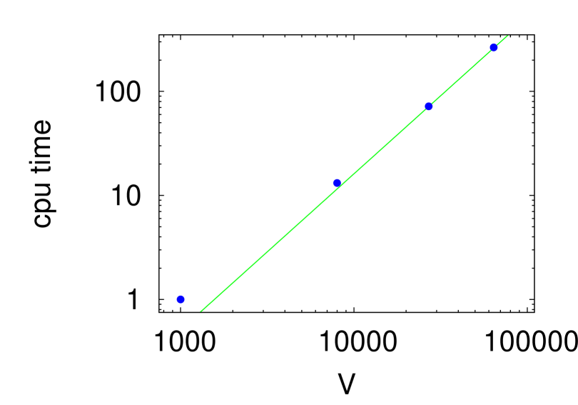
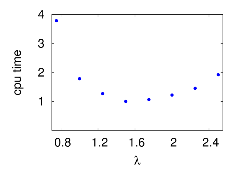
Of course, is only a statement on how to increase , when enlarging the spatial volume . How to choose for a given such that the corresponding computing time is minimized, has to be determined by numerical experiment. In the right panel of Fig. 1 we show in an exemplary plot corresponding to and the computing time needed to calculate the dyon potential as a function of . Obviously, there is an optimal choice for .
Note that in the literature there also exists another version of the just explained “classical Ewald method”, the so-called “particle mesh Ewald method” (cf. e.g. [29]). This version is more efficient, when the interaction energy of a system of positive and negative charges needs to be computed. However, for our problem at hand, the computation of the temporal gauge field , there is no advantage with respect to performance. Since it is significantly simpler to implement, we resort to the classical Ewald method.
For an efficient computation of the short-range sum it is mandatory to determine, which dyons are located in a spherical region of given radius centered around in computer time. To this end we divide the supercell into a grid of cubic subcells and generate for each subcell a list of the contained dyons. In addition we have implemented a function that determines all subcells, which are inside or which intersect the surface of the above mentioned ball. Then we call all those subcells for the dyons they contain. In this way we do not need to inspect all the dyons in the supercell and check whether their distance to is smaller than . Of course, the grid of subcells has to be sufficiently fine-grained, to be able to mimic a ball of radius with rather small cubes.
5 Numerical results
5.1 Extracting the infinite volume string tension using Ewald’s method
We compute the free energy of a static quark-antiquark pair as a function of their separation from Polyakov loop correlators as described in Section 2. We keep the dyon density and the temperature fixed and perform computations for various dyon numbers , corresponding to various spatial volumes of the super cell. The superposition of dyon potentials is calculated by means of the Ewald method as explained in Section 4. We restrict ourselves to maximally non-trivial holonomy.
Of course, the resulting free energies are different for different dyon numbers, i.e. spatial volumes of the super cell, because of finite-volume effects. In particular the dyon potential is -periodic along the three spatial directions, which obviously implies periodic Polyakov loops and loop correlators. Therefore, has to be chosen sufficiently large to ensure that the free energy can be determined for quark-antiquark separations of phenomenological interest, typically a few fm, without being significantly distorted due to periodicity.
| # configurations | ||
|---|---|---|
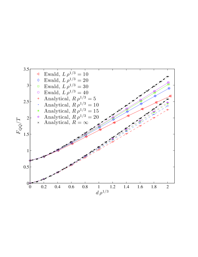
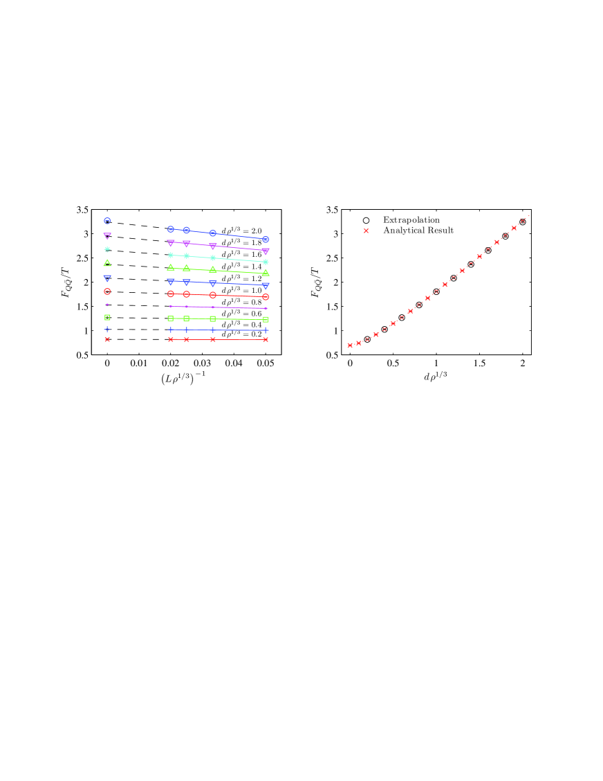
In Fig. 2 we show quark-antiquark free energies for and dyon numbers (corresponding to ) as functions of the quark-antiquark separation . We also show the analytic results for finite and infinite volume in this plot. Note that we express lengths in units of , which is the average dyon separation in a random dyon gas. The number of dyon configurations used for each dyon number is listed in Table 1. It can be seen that the free energies converge, when increasing (or equivalently ). This allows an extrapolation to infinite volume. In the left panel of Fig. 3 we show linear extrapolations of the finite-volume static free energy to infinite volume for a number of quark-antiquark separations. We also compare the results of the extrapolation to the analytically obtained free energy at infinite volume in the right panel of Fig. 3. As can be seen, analytic and extrapolated results nicely agree within errors.
Let us point out that there are other methods of obtaining an infinite volume result numerically without employing Ewald’s summation method.
An obvious method is a straightforward superposition of dyon potentials in a finite cubic box of size , that we call dyon sampling volume. We have used this method in a previous publication [22], to which we refer for further details. Note that there is no exact translational invariance anymore, in contrast to when using periodic boundary conditions via Ewald’s method. To keep finite-volume effects at a tolerable level, we have to restrict the evaluation of Polyakov loops to a spatial subvolume sufficiently far away from the boundary of the dyon volume. We will call this subvolume field sampling volume. It is centered inside the dyon sampling volume and has extension . On the one hand, finite-volume effects are expected to be negligible for sufficiently small . On the other hand, however, decreasing reduces the available information per dyon configuration and, therefore, reduces statistical accuracy. In practice one would need to identify plateaus in the observables as functions of . An obvious and major drawback of proceeding in such a way is that one needs to extrapolate in two parameters, the extension of the sampling volume and the extension of the dyon volume. Clearly this is technically more complicated, than what has to be done using Ewald’s method, where the only parameter subject to extrapolation is the extension of the supercell .
One can also think of evaluating just one Polyakov loop correlator in the center of the volume of each random configuration. We should point out that this is not really feasible if there are interactions, since a significantly larger statistics is needed when no volume averaging is done. For the non-interacting case it is applicable and therefore worth being mentioned.
6 Summary and outlook
In this work we have shown analytically that a non-interacting random dyon gas leads to a linearly rising free energy of a static quark-antiquark pair as a function of the distance in between. Correspondingly the string tension turned out proportional to the ratio of the density and the temperature, i.e. to , cf. Eq. (37). We were able to present explicit formulae for arbitrary distance and for finite volume with certain integrals left to be evaluated numerically. We convinced ourselves that the dependence on the holonomy drops out in the infinite volume limit. This reflects the fact that – concerning the Polyakov loop and its correlator – the model is able to describe only the confinement phase. For the deconfinement transition as well as for the deconfinement phase, where the center symmetry becomes broken, the model should be altered taking into account that dyons with opposite charge should be statistically weighted differently.
We emphasize, that our analytical approach is specific for the non-interacting case. For the interacting case it will not be applicable without approximations, and in the first instance we will have to rely on numerical simulations. Strong finite-size effects of the naive treatment with finite boxes containing the dyon sources have led us to employ a numerical method well-known in the physics of a three-dimensional Coulomb plasma, the Ewald summation method. We convinced ourselves that this method will be applicable also to the more realistic interacting dyon gas.
Indeed, we have demonstrated, how Ewald’s summation method can be used to deal with long-range objects also in field theory, in our case with random ensembles of dyon constituents. In this semiclassically motivated model we have computed the local Polyakov loop, and from its correlator we have extracted the string tension, the main observable characterizing confinement/deconfinement at finite temperature.
The Polyakov loop is a function of an infinite sum of Coulomb contributions of dyons with both signs of charge (cf. Eq. (8)). According to Ewald’s method we have decomposed this sum into short-range and long-range parts, Eqs. (57) and (59), and have optimized the width of the auxiliary Gaussian charge cloud governing the strength of the exponential convergence of both parts.
Figs. 2 and 3 show our main results, the free energy of a quark-antiquark pair as a function of its separation, for various extensions of the (periodically repeated) supercell volume, but fixed dyon density. These figures also demonstrate that the straightforward extrapolation to infinite supercell volume is a valid procedure to obtain results for an infinite non-interacting system of dyons. In this limit the Polyakov loop correlator behaves as expected: it decays exponentially toward larger quark-antiquark separations. The corresponding string tension can be read off unambiguously (and used to fix the physical scale of this model).
We have discussed the advantages of Ewald’s periodic summation over methods that at finite volumes measure observables only in subvolumes: it keeps translational invariance and the infinite volume limit amounts to extrapolating just one parameter.
The applicability of the numerical method we have used is not restricted to a non-interacting dyon ensemble and/or to . Dyon fields in higher gauge groups decay with the distance in the same Coulombic manner, just possessing different color structures. Several other ingredients of dyon models contain Coulomb tails, too, like the interaction of dyons via the action or their moduli space metric. Furthermore, spatial Wilson loops (providing an area law decay with magnetic screening persistent also in the deconfined phase) can – with the help of Stokes’ theorem and based on (anti)selfduality – be represented as area integrals over the normal component of the gradient of the same infinite sum.
The ability to perform a controlled infinite volume extrapolation (with a single remaining parameter , the extension of the periodically continued spatial volume) is even more important in more complicated systems. An ensemble of random dyons could be treated easily with up to dyons. Interacting dyon ensembles are numerically much more expensive such that the reduction to a smaller number of dyons most likely cannot be avoided. Then finite-volume effects might become a limiting factor. Consequently, Ewald’s summation method seems to become indispensable, however, in form of the particle mesh Ewald method, which is more efficient than the classical Ewald method, when computing dyon interactions.
Appendix A Calculation of some integrals
We derive the following results for the integrals and involved in Polyakov loop correlators in Section 3.2,
| (60) | |||||
| (61) |
In the first integral we use the well-known Fourier representation of the Coulomb potential
| (62) |
to calculate
| (63) | |||||
The Laplace operator can be used to check this result. Acting with respect to and on the left hand side we obtain (from the mixed term in the integrand)
| (64) | |||||
On the right hand side it gives the same since
| (65) |
The integrand of the second integral is positive, which proves the first inequality. For the second inequality we split -space into two half-spaces, , separated by the midplane between the two points and . The integral over each half-space gives half of the full integral and thus we can specify to one of them, e.g. where
| (66) |
holds. Since the integrand is monotonically increasing for , we obtain an upper bound
| (67) | |||||
Due to the positivity of the integrand, we can extend the latter integral back to the full space and by virtue of translational invariance put obtaining another bound
| (68) | |||||
independently of , by which we have proven the second inequality.
Appendix B Ewald’s sum compared with summing over a finite array of supercells
Ewald’s method amounts to summing over infinitely many copies of the cubic spatial volume called supercell. An alternative approach is to truncate this sum after a large but finite number of copies in every spatial direction , and . The corresponding dyon potential obtained by summing over copies of the supercell is then
| (69) |
where and . One might expect that, when is chosen sufficiently large, the Ewald result, denoted by , and become arbitrarily close. In this section we explain that this is not the case, i.e. that even though converges, when increasing , it will in general differ from .
The difference between the two approaches is
| (70) |
In the following we demonstrate by means of a simple example that in general. To this end consider , a dyon () at position and an antidyon () at position .
For dyons and antidyons in (70) cancel exactly with exception of antidyons/dyons located on planes at , . Since the dyon potential is identical to the potential of an electric charge in classical electrostatics, the situation is reminiscent to that of a uniformly polarized cubic dielectric with volume . For the discrete charges can be approximated by the surface charge density at the two opposite sides .
For the dyon and antidyon potentials only partly cancel resulting in a reduced surface charge density .
For the difference is given by
| (71) |
i.e.
| (72) |
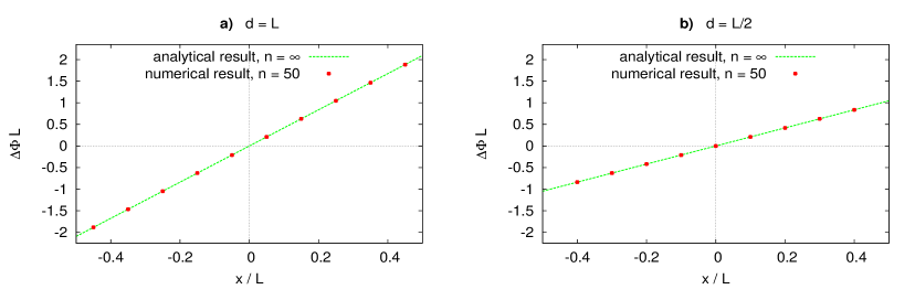
In Fig. 4 we show that this analytical result is accurately reproduced by our numerical implementation of Ewald’s method and the finite sum (69) using .
For a larger number of dyons with arbitrary positions is, of course, rather hard to estimate analytically. The physical picture, however, will remain the same: like in a polarized dielectric surface charges will cause a difference between and . Only in the limit corresponding to both approaches are expected to become identical.
In principle both approaches can be used to simulate dyon ensembles, since, after appropriately extrapolating the dyon number (or alternatively ), one should obtain the same correct infinite volume result. We consider, however, Ewald’s method to be superior, because in this approach the spatial volume is translationally invariant. This allows to maximally exploit a given dyon gauge field configuration by evaluating observables throughout the whole spatial volume. In contrast to that, translational invariance is broken when truncating the sum over copies of the super cell. Observables must only be evaluated in regions, where this breaking is sufficiently mild. Each observable requires to determine a corresponding region of sufficiently mild finite volume effects. Moreover, one has to assure that the associated systematic is removed by the infinite volume extrapolation.
Acknowledgments
The authors express their gratitude for financial support by the German Research Foundation (DFG) with various grants: F.B. with grant BR 2872/4-2, S.D. by the corroborative research center SFB/TR9, E.-M.I. and M.M.-P. with grant Mu 932/6-1, as well as M.W. by the Emmy Noether Programme with grant WA 3000/1-1.
References
- [1] C. G. Callan Jr, R. F. Dashen, and D. J. Gross, Phys. Rev. D17, 2717 (1978).
- [2] C. G. Callan Jr, R. F. Dashen, and D. J. Gross, Phys. Rev. D19, 1826 (1979).
- [3] A. A. Belavin, A. M. Polyakov, A. S. Shvarts, and Y. S. Tyupkin, Phys. Lett. B59, 85 (1975).
- [4] T. Schäfer and E. V. Shuryak, Rev. Mod. Phys. 70, 323 (1998), hep-ph/9610451.
- [5] D. Diakonov, Prog. Part. Nucl. Phys. 51, 173 (2003), hep-ph/0212026.
- [6] T. C. Kraan and P. van Baal, Nucl. Phys. B533, 627 (1998), hep-th/9805168.
- [7] T. C. Kraan and P. van Baal, Phys. Lett. B435, 389 (1998), hep-th/9806034.
- [8] K.-M. Lee and C.-H. Lu, Phys. Rev. D58, 025011 (1998), hep-th/9802108.
- [9] P. Ewald, Ann. Phys. 369, 253 (1921).
- [10] B. J. Harrington and H. K. Shepard, Phys. Rev. D17, 2122 (1978).
- [11] P. Gerhold, E.-M. Ilgenfritz, and M. Müller-Preussker, Nucl. Phys. B760, 1 (2007), hep-ph/0607315.
- [12] D. Diakonov, N. Gromov, V. Petrov, and S. Slizovskiy, Phys. Rev. D70, 036003 (2004), hep-th/0404042.
- [13] T. C. Kraan, Commun. Math. Phys. 212, 503 (2000), hep-th/9811179.
- [14] D. Diakonov and N. Gromov, Phys. Rev. D72, 025003 (2005), hep-th/0502132.
- [15] F. Bruckmann, E.-M. Ilgenfritz, B. Martemyanov, and B. Zhang, Phys. Rev. D81, 074501 (2010), 0912.4186.
- [16] N. S. Manton, Phys. Lett. B154, 397 (1985).
- [17] G. W. Gibbons and N. S. Manton, Nucl. Phys. B274, 183 (1986).
- [18] G. W. Gibbons and N. S. Manton, Phys. Lett. B356, 32 (1995), hep-th/9506052.
- [19] D. Diakonov and V. Petrov, Phys. Rev. D76, 056001 (2007), 0704.3181.
- [20] D. Diakonov, Nucl.Phys.Proc.Suppl. 195, 5 (2009), 0906.2456.
- [21] A. M. Polyakov, Nucl. Phys. B120, 429 (1977).
- [22] F. Bruckmann, S. Dinter, E.-M. Ilgenfritz, M. Müller-Preussker, and M. Wagner, Phys. Rev. D79, 116007 (2009), 0903.3075.
- [23] V. Bornyakov, E.-M. Ilgenfritz, B. Martemyanov, and M. Müller-Preussker, Phys.Rev. D79, 034506 (2009), 0809.2142.
- [24] F. Bruckmann, PoS CONFINEMENT8, 179 (2008), 0901.0987.
- [25] A. M. Polyakov, Phys. Lett. B72, 477 (1978).
- [26] S. Digal, S. Fortunato, and P. Petreczky, Phys.Rev. D68, 034008 (2003), hep-lat/0304017.
- [27] B. Lucini, M. Teper, and U. Wenger, JHEP 02, 033 (2005), hep-lat/0502003.
- [28] H. Lee and W. Cai, 2009, Lecture Notes, Stanford University, 2009.
- [29] U. Essmann et al., J. Chem. Phys. 103, 8577 (1995).
- [30] F. Lenz, J. W. Negele, and M. Thies, Phys. Rev. D69, 074009 (2004), hep-th/0306105.
- [31] F. Lenz, J. W. Negele, and M. Thies, Annals Phys. 323, 1536 (2008), 0708.1687.
- [32] M. Wagner, Phys. Rev. D75, 016004 (2007), hep-ph/0608090.
- [33] C. Szasz and M. Wagner, Phys. Rev. D78, 036006 (2008), 0806.1977.