Current noise spectrum of a single particle emitter: theory and experiment

Abstract

The controlled and accurate emission of coherent electronic wave packets is of prime importance for future applications of nano-scale electronics. Here we present a theoretical and experimental analysis of the finite-frequency noise spectrum of a periodically driven single electron emitter. The electron source consists of a mesoscopic capacitor that emits single electrons and holes into a chiral edge state of a quantum Hall sample. We compare experimental results with two complementary theoretical descriptions: On one hand, the Floquet scattering theory which leads to accurate numerical results for the noise spectrum under all relevant operating conditions. On the other hand, a semi-classical model which enables us to develop an analytic description of the main sources of noise when the emitter is operated under optimal conditions. We find excellent agreement between experiment and theory. Importantly, the noise spectrum provides us with an accurate description and characterization of the mesoscopic capacitor when operated as a periodic single electron emitter.

I Introduction

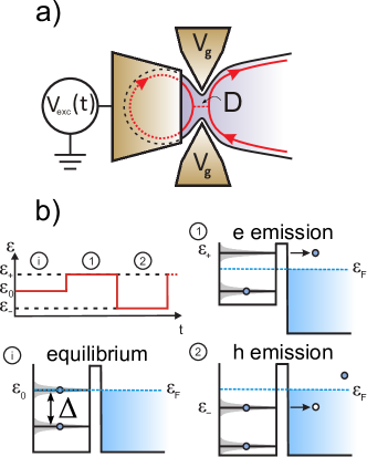
Figure 1: (color online). The mesoscopic capacitor. a) Schematic representation of the mesoscopic capacitor. A quantum point contact (with gate voltage $V_{\mathrm{g}}$ controlling the transparency $D$) couples the edge channels (red arrows) in the capacitor and in the electron gas. Electron/hole emission is triggered by the excitation drive $V_{exc}(t)$ applied to the capacitor top gate. b) Principle of single charge emission (in the non-adiabatic regime) using the mesoscopic capacitor. At \protect\raisebox{-1.2pt}{i}⃝ the capacitor is at equilibrium and the highest occupied level (HOL) is resonant with the Fermi level of the electron gas $\epsilon_{\mathrm{F}}$ (dashed blue line). The level spacing is denoted as $\Delta$. \protect\raisebox{-1.2pt}{1}⃝ is electron emission phase: the HOL is promoted far above the Fermi energy, causing the capacitor to emit the electron through the quantum point contact. \protect\raisebox{-1.2pt}{2}⃝ is the hole emission phase: the emptied level is brought far below the Fermi energy of the external reservoir and an electron is absorbed from the electron gas, i. e. a single hole is emitted. A continuous repetition of the sequence \protect\raisebox{-1.2pt}{1}⃝$\leftrightarrow$\protect\raisebox{-1.2pt}{2}⃝ results in periodic emission of a single electron followed by a single hole. This corresponds to the optimal operating condition of the emitter.

The development of on-demand single electron emitters opens a promising route towards novel nano-scale electronics based on the coherent manipulation of only a single or a few electronic wave packets. The chiral edge channels of the integer quantum Hall effect (IQHE), obtained when a strong perpendicular magnetic field is applied to a two-dimensional electron gas, constitute an ideal experimental setup to test these new concepts in the design of quantum electronic circuits. It is now possible to fabricate micron-sized electrical networks in which the propagation of electrons is truly one-dimensional, ballistic, and quantum coherent, thus mimicking the propagation of photons in optical fibers. Moreover, by depositing metallic split gates on top of the electron gas, quantum point contacts acting as tunable electron beam splitters can also be implemented. Using continuous particle sources, single electron interferences have already been observed in electronic Mach-Zehnder interferometers Ji2003 ; Litvin2007 ; Roulleau2008 , as well as two-electron interferences in similar systems Neder ; Sam2004 ; Samuelsson2009 . However, for experiments or applications where the timing of wave packets is important, e. g. for interference experiments that require particles to arrive simultaneously at the scatterer, continuous sources are not useful as one cannot control the emission time of electrons into the conductor. Continuous sources then need to be replaced by triggered emittersFeve2007 ; Blum2007 ; PekolaNP2008 ; Giazotto2011 ; LeichtSST2011 ; HermelinNat2011 ; McNeil2011 that can produce single particle states in a controllable and timed manner.

A prime example of a single electron emitter is the periodically driven mesoscopic capacitor, consisting of a sub-micron cavity coupled to an edge state. The device was first theoretically proposed by Büttiker et al. Buttiker1993 who showed that the relaxation resistance is quantized in units of $h/2e^{2}$ independently of microscopic details Nig2006 ; But2007b ; Ringel2008 ; Mora2010 ; Hamamoto2010 ; Splettstoesser2010 ; Filippone2011 ; Lee2011 . Experimentally, this prediction was confirmed by Gabelli et al. Gabelli2006 . In a subsequent experiment, Fève et al. showed that the mesoscopic capacitor, when subject to large periodic gate voltage modulations, can absorb and re-emit single electrons at gigahertz frequencies, generating a quantized AC current Feve2007 . Several proposals have been made to coherently manipulate the single electron states emitted by such a source in order to observe two-electron interferences Ol'khovskaya ; Juergens2011 or electron entanglement Splettstoesser2009 . The use of two-particle exchange effects has also been suggested as a means to visualize the single electron states generated by the source in a tomography protocol Gre10 ; TheseGrenier allowing for a direct characterization of the interaction between a single electronic excitation and its environment Degio2009 . Coherence properties of the single electron states emitted by the source can also be analyzed by injecting particles into a Mach-Zehnder interferometer Haack2011 . However, in order to facilitate these few-fermion experiments, it is necessary first to accurately characterize and understand in detail the single electron emission process. The average current measurements performed so far in Refs. Feve2007, and Blum2007, give access to the average behavior of the source after a large number of particle emissions, but are not designed to provide information about the elementary processes involved in a single emission event. For example, average current measurements cannot distinguish between the deterministic emission of exactly one electron followed by one hole during each period of the external driving and a fluctuating number of emitted particles from cycle to cycle which still results in the same number of emitted charges after many periods. The statistical properties of the source may be characterized by measuring the full counting statistics Levitov93 ; Nazarov2003 of electron emissions, but in this case as well, the short time behavior of the emitter is not accessible. In contrast, as recently suggested by some of us, the waiting time distribution Albert2011 between individual charge events would provide information about the short-time physics, but an actual measurement of the waiting time distribution still remains an open and experimentally challenging task.

We focus in this work on the short time current-current correlations (or frequency-dependent noise) as an experimental tool to describe and characterize the elementary excitations generated by the mesoscopic capacitor when operated as a periodic single electron source. In two recent short papers we have separately presented measurementsMahe2010 and theory Albert2010 of the finite-frequency current noise of the mesoscopic capacitor. In the present work, we expand significantly on the theoretical calculations of the current noise and compare the recent measurements of the high-frequency noise Mahe2010 to two complementary theoretical descriptions: on one hand, the full-fledged Floquet scattering theory Moskalets2002 ; Moskalets2007 ; Moskalets2008 which naturally applies to periodically driven systems and gives highly accurate numerical results for the current noise, and on the other hand, a conceptually simple semi-classical model Mahe2010 ; Albert2010 which shows surprisingly good agreement with the experiment and additionally provides us with a simple intuitive picture of the dynamical emission processes. Based on the excellent agreement between the measurements of the short time current-current correlations and the two theoretical descriptions we provide a detailed characterization of the single electron emitter. In particular, we can identify parameter regimes for which nearly perfect and deterministic single electron-hole emission is achieved in every cycle. For details of the experiment we refer the interested reader to Ref. Mahe2010, .

The paper is now organized as follows: In Sec. II we introduce the mesoscopic capacitor and describe the basic operating principles that enable periodic emission of electron-hole pairs into an edge state. Sec. III gives an elaborate account of the Floquet scattering theory applied to the mesoscopic capacitor and we discuss calculations of the average current and the current noise both for a two- and a three-terminal configuration. We employ a non-interacting model which allows us to consider all possible parameter ranges and operating conditions. Sec. IV compares theoretical predictions of the Floquet scattering theory with experimental data of the average current. In Sec. V we present a semi-classical model that describes the mesoscopic capacitor around the operating conditions, where maximally one charge (electron or hole) is emitted in each half-cycle. The semi-classical model allows us to account analytically for two important sources of noise: when electron and hole emissions become rare, the current fluctuations are shot-noise like and the noise spectrum is white. In contrast, close to the optimal operating regime, where exactly one electron-hole pair is emitted in each cycle, the current fluctuations are dominated by the randomness of the emission times within a period, giving rise to phase noise with a Lorentzian-like noise spectrum. In Sec. VI we exhaustively compare measurements, Floquet scattering theory, and the semi-classical model, focusing both on current and noise in different parameter regimes including the shot noise and phase noise dominated limits. We discuss the general properties of the noise of the single electron emitter as well as the deviations between the Floquet scattering theory and the semi-classical model when the mesoscopic capacitor is operated away from the optimal conditions. Finally, in Sec. VII we present our concluding remarks.

II Mesoscopic capacitor

The mesoscopic capacitor is depicted in Fig. 1. It consists of a submicron-sized cavity (or quantum dot) coupled to a two-dimensional electron gas through a quantum point contact (QPC) whose transparency $D$ is controlled by the gate voltage $V_{\mathrm{g}}$. A capacitively coupled metallic top-gate controls the static offset potential in the dot $V_{0}$, as well as the rapidly oscillating component $V_{\mathrm{exc}}(t)$ generated by radio-frequency excitations. A large perpendicular magnetic field is applied to the sample, so that electrons propagate along the one-dimensional chiral edge channels that form due to the IQHE. The system can in principle be operated at an arbitrary integer value of the filling factor $\nu$ in the electron gas (typically $\nu=4$), but in any case only the outer edge channel couples to the quantum dot. Electrons propagating along the outer edge channel of the quantum dot experience a discrete energy spectrum with energy levels that are separated by a constant level spacing $\Delta$, see Fig. 1b. The levels are broadened by the finite coupling between the quantum dot and the electron gas, determined by the QPC transmission $D$. Interaction effects within the quantum dot were not experimentally observedFeve2007 and are thus neglected throughout this work (the absence of Coulomb interactions may be due to the screening from the large metallic top gate as well as the presence of the inner edge channels in the quantum dot).

Without the periodic driving $V_{\mathrm{exc}}(t)$ (corresponding to the equilibrium situation denoted as \protect\raisebox{-1.2pt}{i}⃝ in Fig. 1b), the position of the energy levels with respect to the Fermi energy is determined by the constant voltage $V_{0}$ applied to the top-gate: this top-gate voltage fixes the position of the highest occupied level $\epsilon_{0}$ (HOL) with respect to the Fermi energy $\epsilon_{\mathrm{F}}$ at equilibrium. Adding next the pure AC excitation voltage $V_{\mathrm{exc}}(t)$ causes the HOL to be periodically shifted up and down with respect to its equilibrium position. We consider the situation realized experimentally Feve2007 ; Mahe2010 , where a square shape excitation is applied, causing sudden shifts of the quantum dot energy spectrum. The square shape excitation contains a broad range of Fourier components and is thus a non-adiabatic excitation with respect to all relevant time and energy scales. If the peak-to-peak amplitude of the excitation drive $2eV_{\mathrm{exc}}$ is comparable to the level spacing $\Delta$, the HOL is promoted to an energy $\epsilon_{+}$ far above the Fermi level in the first half-period of the drive (labeled as \raisebox{-1.2pt}{1}⃝ in Fig. 1b), where the electron occupying the level is then emitted to the electron gas through the quantum point contact. In the following half-period (labeled as \raisebox{-1.2pt}{2}⃝), the emptied level is next brought to an energy $\epsilon_{-}$ far below the Fermi energy, where an electron is absorbed from the electron gas (corresponding to the emission of a hole as indicated in Fig. 1). Repeating the sequence \raisebox{-1.2pt}{1}⃝$\leftrightarrow$\raisebox{-1.2pt}{2}⃝ at a drive frequency of $f_{d}\approx 1$ GHz thus gives rise to periodic emission of a single electron followed by a single hole.

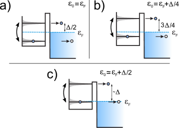
Figure 2: (color online). Different operating conditions for the mesoscopic capacitor. Only the HOL is shown; the curved arrow represents the AC drive (with amplitude $2eV_{\mathrm{exc}}=\Delta$) which periodically and abruptly shifts the HOL above and below the Fermi level $\epsilon_{\mathrm{F}}$ (dashed blue line). The dotted arrow denotes the energy of the emitted electron measured with respect to the Fermi level. a) Optimal operating condition: the energy of the HOL without driving field $V_{\mathrm{exc}}$ equals the Fermi energy of the electron gas, $\epsilon_{0}=\epsilon_{\mathrm{F}}$. With the driving field applied, the electron (hole) is then emitted at $\Delta/2$ above (below) the Fermi level $\epsilon_{\mathrm{F}}$. b) Intermediate case with $\epsilon_{0}=\epsilon_{\mathrm{F}}+\Delta/4$: the electron (hole) is emitted at $3\Delta/4$ ($\Delta/4$) above (below) the Fermi level. c) Non-optimal operating condition with $\epsilon_{0}\approx\epsilon_{\mathrm{F}}+\Delta/2$: the electron is then emitted at $\sim\Delta$ above the Fermi level, while the hole is emitted on resonance with $\epsilon_{\mathrm{F}}$. In this case, emissions of spurious electron-hole pairs lead to unwanted electrical fluctuations.

Obviously, the discussion above depends crucially on the value of the static potential $V_{0}$, which fixes the equilibrium position $\epsilon_{0}$ of the HOL and thus the positions $\epsilon_{+}$ and $\epsilon_{-}$ during the electron emission (\raisebox{-1.2pt}{1}⃝) and hole emission (\raisebox{-1.2pt}{2}⃝) phases, respectively, Indeed, as illustrated in Fig. 2, for certain values of $\epsilon_{0}$, the HOL may be in resonance with the Fermi level during one of the two phases. Such a situation is depicted in Fig. 2c, where $\epsilon_{0}\approx\epsilon_{\mathrm{F}}+\Delta/2$ and $2eV_{\mathrm{exc}}=\Delta$, resulting in $\epsilon_{+}\approx\epsilon_{\mathrm{F}}+\Delta$ and $\epsilon_{-}\approx\epsilon_{\mathrm{F}}$. Thus, during the hole emission phase, the HOL is resonant with the Fermi level, and several charges can be absorbed and re-emitted during a single hole emission phase (note that during the electron emission phase, the second occupied level is also resonant with the Fermi energy). As predicted in Ref. Keeling2008, , such emissions of spurious electron-hole pairs degrade the quality of the single particle source and lead to unwanted electrical fluctuations. In this respect, the optimal operating conditions of the emitter are obtained when the HOL is alternatively brought far above and below the Fermi level $\epsilon_{\mathrm{F}}$ during the emission cycle. Two such cases are shown in Fig. 2a and b. However, even under these favorable conditions, a too large value of the QPC transmission $D$ may broaden the level so much that it starts to overlap with the Fermi energy of the lead. The optimal operating conditions are therefore determined by a subtle interplay between the static potential $V_{0}$, the amplitude of the AC drive $V_{\mathrm{exc}}$, and the transmission probability $D$ of the QPC.

III Floquet scattering theory

We now describe the Floquet scattering matrix theory used to calculate numerically the average current and the finite-frequency noise of the periodically driven mesoscopic capacitor. After a general presentation of the formalism, we apply it to calculate the current and noise in the experimental situations considered in this work.

III.1 Description of the system

We consider the schematic setup depicted in Fig. 3. Electrons in the incoming edge channel can tunnel onto the quantum dot with the amplitude $\sqrt{D}=\sqrt{1-r^{2}}$, perform several round-trips inside the mesoscopic capacitor, each taking the finite time $\tau_{o}=l/v_{d}$, before finally tunneling back out into the out-going edge state. In these expressions, the reflection amplitude $r$ has for convenience been assumed to be real and energy-independent, while $l$ and $v_{d}$ are the circumference of the quantum dot and the drift velocity, respectively. In this setup, the quantum dot acts as an electronic analog of a Fabry-Pérot cavity.

We first consider the simple situation, where only a static potential $V_{0}$ is applied to the quantum dot. The creation $\hat{b}^{\dagger}(t)$ and annihilation $\hat{b}(t)$ operators for an outgoing state at time $t$ are then related to the creation $\hat{a}^{\dagger}(t^{\prime})$ and annihilation $\hat{a}(t^{\prime})$ operators for an incoming state at time $t^{\prime}$ through the Fabry-Pérot phase acquired after scattering on the quantum dot

$$\begin{split}\hat{b}(t)&=\int dt^{\prime}U(t,t^{\prime})\hat{a}(t^{\prime}),\\ U(t,t^{\prime})&=r\delta(t-t^{\prime})\\ &-D\sum_{q=1}^{\infty}r^{q-1}\delta(t-t^{\prime}-q\tau_{o})e^{-ieV_{0}q\tau_{o}/\hbar}.\end{split}$$ (1)

Here, $eV_{0}\tau_{o}/\hbar$ is the phase acquired during a single round-trip inside the quantum dot and $e$ is the electron charge. In the Fourier domain, the creation $\hat{b}^{\dagger}(\epsilon)$ and annihilation $\hat{b}(\epsilon)$ operators for the outgoing states are related to the operators of the incoming states $\hat{a}^{\dagger}(\epsilon)$ and $\hat{a}(\epsilon)$ at energy $\epsilon=\hbar\omega$ through the stationary scattering matrix $\mathcal{S}(\epsilon)$:

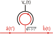
Figure 3: (color online). Schematic representation of the mesoscopic capacitor as a time-dependent scatterer. Electrons in the in-going edge channel are scattered on the quantum dot (red loop) subject to the time-dependent potential $V_{\mathrm{exc}}(t)$.

$$\begin{split}\hat{a}(\epsilon)&=\int\frac{dt}{\sqrt{h}}e^{i\epsilon t/\hbar}\hat{a}(t),\\ \hat{b}(\epsilon)&=\mathcal{S}(\epsilon)\hat{a}(\epsilon),\\ \mathcal{S}(\epsilon)&=\frac{r-e^{i\tau_{o}(\epsilon-\epsilon_{0})/\hbar}}{1-re^{i\tau_{o}(\epsilon-\epsilon_{0})/\hbar}}.\end{split}$$ (2)

The density of states of the quantum dotButtiker1994

$$\rho(\epsilon)=\frac{1}{2\pi i}\mathcal{S}^{\ast}(\epsilon)\frac{d\mathcal{S}}{d\epsilon}$$ (3)

consists of a series of peaks corresponding to the discrete energy levels of the quantum dot. The typical level spacing $\Delta=h/\tau_{o}$ is on the order of a few Kelvins. The levels are broadened by the coupling to the electron gas with the width of the peaks given by $D\Delta/(2\pi)$. The static potential $\epsilon_{0}=eV_{0}$ shifts the position of the energy levels measured with respect to the Fermi energy $\epsilon_{\mathrm{F}}$ which we thus freely can set to zero, $\epsilon_{\mathrm{F}}=0$, throughout the rest of the paper. The potential shift can be written as a phase factor $\phi=\epsilon_{0}\tau_{o}/\hbar$ entering the expression for the stationary scattering matrix $\mathcal{S}(\epsilon)$. This allows us to describe the position of the levels in the dot at equilibrium independently of the level spacing $\Delta$; in particular, for $\phi=0$ ($\epsilon_{0}=0$), the highest occupied level is resonant with the Fermi energy at equilibrium, whereas for $\phi=\pi$ ($\epsilon_{0}=\Delta/2$), the Fermi energy lies midway in between the highest occupied level and the lowest unoccupied level.

In order to induce a finite AC current in the out-going edge channel, one must consider a time-dependent modulation of the quantum dot potential. In addition to the static potential $V_{0}$, we therefore consider a periodic modulation $V_{\mathrm{exc}}(t)$ with no dc component. The period of the modulations is $T=1/f_{d}=2\pi/\Omega$, which also defines the drive frequency $f_{d}$. The quantum dot can now be viewed as a time-dependent periodic scatterer, which can be conveniently described using the Floquet scattering matrix formalismMoskalets2002 . Between times $t-q\tau_{o}$ and $t$, an electron inside the quantum dot performs $q$ round trips, during which it experiences the time-dependent potential $V_{\mathrm{exc}}(t)$. The electron then acquires an additional phaseMoskalets2008 $\Delta\phi=\frac{e}{\hbar}\int_{t-q\tau_{o}}^{t}V_{\mathrm{exc}}(t^{\prime})dt^{\prime}$. Since the drive $V_{\mathrm{exc}}(t)$ is periodic, we can express the acquired phase in terms of the Fourier coefficients $c_{n}$ entering the Fourier series

$$e^{-i\frac{e}{\hbar}\int_{0}^{t}V_{\mathrm{exc}}(t^{\prime})dt^{\prime}}=\sum_{n}c_{n}e^{-in\Omega t}.$$ (4)

The annihilation operators $\hat{b}(\epsilon)$ and $\hat{a}(\epsilon^{\prime})$ then become related as

$$\begin{split}\hat{b}(\epsilon)&=\int d\epsilon^{\prime}U(\epsilon,\epsilon^{\prime})\hat{a}(\epsilon^{\prime}),\\ U(\epsilon,\epsilon^{\prime})&=\sum_{n,m}c_{n}c^{*}_{n+m}\mathcal{S}(\epsilon-n\hbar\Omega)\delta(\epsilon-\epsilon^{\prime}+m\hbar\Omega)\\ &=\sum_{m}U_{m}(\epsilon)\delta(\epsilon-\epsilon^{\prime}+m\hbar\Omega).\end{split}$$ (5)

The Floquet scattering theory clearly expresses how scattering occurs through the emission or absorption of a quantized number $m$ of energy quanta $\hbar\Omega$Shirley1965 . The scattering amplitude associated with the transfer of $m$ quanta is given by the Floquet scattering matrix $U_{m}(\epsilon)$ ,

$$\begin{split}\hat{b}(\epsilon)&=\sum_{m}U_{m}(\epsilon)\hat{a}(\epsilon_{m}),\\ U_{m}(\epsilon)&=\sum_{n}c_{n}c^{*}_{n+m}\mathcal{S}(\epsilon_{-n}),\end{split}$$ (6)

where the notation

$$\epsilon_{\pm m}=\epsilon\pm m\hbar\Omega$$ (7)

has been introduced for convenience. We note that in the absence of the excitation drive, only elastic processes can occur and we recover $U_{m}(\epsilon)=\mathcal{S}(\epsilon)\delta_{m,0}$ in agreement with Eq. (2). Finally, from the unitarity of the time evolution operator $U$, the following relations can be deduced:

$$\begin{split}\sum_{n}U_{n+p}^{*}(\epsilon_{-p})U_{n+p^{\prime}}(\epsilon_{-p^{\prime}})=\delta_{p,p^{\prime}}\\ \sum_{n}U_{n+p}^{*}(\epsilon_{-n})U_{n+p^{\prime}}(\epsilon_{-n})=\delta_{p,p^{\prime}}\end{split}$$ (8)

III.2 Experimental considerations

With the Floquet scattering matrices at hand we can now proceed with calculations of the average current and the finite-frequency noise. At this point, however, the experimental details of the measurement setup must be carefully considered. In Fig. 4 we show a two and a three-terminal experimental setup. In the two-terminal geometry, Fig. 4a, the incoming and outgoing edge channels are connected to the same ohmic contact with a fixed chemical potential taken as the zero-energy reference $\mu=\epsilon_{\mathrm{F}}=0$. The top-gate of the quantum dot is considered as the second terminal. The two-terminal setup suffices for measurements of the average current.

However, for measurement of the current noise it is useful to include an additional ohmic contact as shown in Fig. 4b. The additional ohmic contact is inserted between the measurement contact and the quantum dot and is connected to a cold mass. In this geometry, the noise is measured on a constant impedance, given by the edge channels flowing from the measurement contact to the grounded contact GlattliEPJST2009 . The impedance of the sample seen by the detection circuit is therefore independent of the parameters of the quantum dot and, in particular, of the QPC transmission $D$. The environmental noise (noise of the amplifier or thermal noise emitted by the detection circuit towards the sample) is reflected on a constant impedance and is therefore easily subtracted in order to extract the noise emitted by the source as we discuss in detail below. Only the noise due to the capacitor is then measured.

III.2.1 Two-terminal geometry

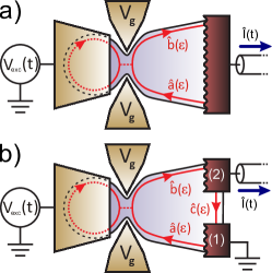
Figure 4: (color online). Experimental setups. a) Two-terminal geometry in which the incoming and outgoing edge channels (red arrows) are both connected to the same ohmic contact, where the current is measured. b) Three-terminal geometry in which the incoming and outgoing edge states (red arrows) are connected to ohmic contacts $1$ and $2$, respectively. The current is measured in contact $2$.

For the two-terminal geometry in Fig. 4a, the operator for the current emitted by the contact is given as

$$\begin{split}\hat{I}(t)&=e\big{[}\hat{b}^{{\dagger}}(t)\hat{b}(t)-\hat{a}^{{\dagger}}(t)\hat{a}(t)\big{]},\\ &=\frac{e}{h}\int d\epsilon\;d\epsilon^{\prime}e^{i(\epsilon-\epsilon^{\prime})t/\hbar}\Big{[}\hat{b}^{{\dagger}}(\epsilon)\hat{b}(\epsilon^{\prime})-\hat{a}^{{\dagger}}(\epsilon)\hat{a}(\epsilon^{\prime})\Big{]}\\ &=\frac{e}{h}\int d\epsilon d\epsilon^{\prime}\;e^{i(\epsilon-\epsilon^{\prime})t/\hbar}\\ &\times\Big{[}\sum_{m,m^{\prime}}U^{*}_{m}(\epsilon)U_{m^{\prime}}(\epsilon^{\prime})a^{{\dagger}}(\epsilon_{m})a(\epsilon^{\prime}_{m^{\prime}})-a^{{\dagger}}(\epsilon)a(\epsilon^{\prime})\Big{]}.\end{split}$$ (9)

Since the ohmic contact is in thermal equilibrium with temperature $T_{\mathrm{el}}$ and chemical potential $\mu=0$, we have

$$\langle\hat{a}^{{\dagger}}(\epsilon)\hat{a}(\epsilon^{\prime})\rangle=f(\epsilon)\delta(\epsilon-\epsilon^{\prime}),$$ (10)

where $f(\epsilon)$ is the Fermi-Dirac distribution. The average current $\langle\hat{I}(t)\rangle$ has the same $T$-periodicity as the driving potential $V_{\mathrm{exc}}(t)$ and can therefore be written in terms of its Fourier components $I_{k}$ as

$$\langle\hat{I}(t)\rangle=\sum_{k}e^{ik\Omega t}I_{k},$$ (11)

where

$$I_{k}=\frac{e}{h}\!\sum_{\ell}\!\int\!d\epsilon U^{*}_{\ell}(\epsilon)U_{\ell+k}(\epsilon_{-k})\big{[}f(\epsilon_{\ell})-f(\epsilon)\big{]}\,.$$ (12)

In particular, the first harmonic $I_{\Omega}=I_{k=1}$ is given by

$$I_{\Omega}=\frac{e}{h}\sum_{\ell}\int d\epsilon U^{*}_{\ell}(\epsilon)U_{\ell+1}(\epsilon-\hbar\Omega)\big{[}f(\epsilon+\ell\hbar\Omega)-f(\epsilon)\big{]}.$$ (13)

We consider next the noise emitted by the source in the two-terminal geometry using the expressions for the current operator $\hat{I}(t)$ in Eq. (9). Since $\hat{I}(t)$ corresponds to a non-stationary current, the current-current correlation function

$$C(t,t^{\prime})=\langle\delta\hat{I}(t)\delta\hat{I}(t+t^{\prime})\rangle,$$ (14)

with $\delta\hat{I}(t)=\hat{I}(t)-\langle\hat{I}(t)\rangle$, depends explicitly both on the absolute time $t$ as well as the time difference $t^{\prime}$. The current-current correlation function is $T$-periodic in the absolute time $t$, such that it can be expressed in terms of the Fourier components $C_{l}(t^{\prime})$ as

$$C(t,t^{\prime})=\sum_{l}e^{il\Omega t}C_{l}(t^{\prime}).$$ (15)

Experimentally, the current noise spectrum is averaged over the absolute time $t$, and only the Fourier component $C_{0}(t^{\prime})$ is measured. In the frequency domain we have $\mathcal{P}_{0}(\omega)=\int dt^{\prime}e^{i\omega t^{\prime}}C_{0}(t^{\prime})$ with the mean power spectral density for $\omega>0$ defined as

$$S(\omega)=2\int dt^{\prime}\overline{\langle\delta I(t)\delta I(t+t^{\prime})\rangle}^{t}e^{i\omega t^{\prime}}=2\mathcal{P}_{0}(\omega).$$ (16)

The symbol $\overline{\cdot\cdot\cdot}^{t}$ denotes averaging over $t$. The noise for the two-terminal geometry $S_{2T}(\omega)$ contains a contribution from the cross-correlations of the current flowing from the contact, $\hat{I}_{a}(t)=e\hat{a}^{{\dagger}}(t)\hat{a}(t)$, and the current flowing into the contact, $\hat{I}_{b}(t)=e\hat{b}^{{\dagger}}(t)\hat{b}(t)$ as well as contributions from the autocorrelations of $\hat{I}_{a}$ and $\hat{I}_{b}$. The operators $\hat{I}_{b}$ and $\hat{I}_{a}$ are related through the Floquet scattering matrix $U_{m}(\epsilon)$, and after some algebra we arrive at

$$S_{2T}(\omega)=\frac{2e^{2}}{h}\sum_{m}\int d\epsilon\left|\delta_{m,0}-\sum_{n}U^{\ast}_{n}(\epsilon_{-n})U_{n+m}(\epsilon_{-n}-\hbar\omega)\right|^{2}f(\epsilon)\Big{(}1-f(\epsilon_{m}+\hbar\omega)\Big{)}.$$ (17)

Equations (11-12) and (17) are useful for numerical calculations of the average current and the finite-frequency noise, respectively, for the two-terminal geometry.

III.2.2 Three-terminal geometry

We next consider the three-terminal geometry depicted in Fig. 4b. In this case, electronic wave packets incident on the quantum dot have been emitted from contact $1$, whereas the electronic waves scattering off the quantum dot are collected in contact $2$. The total current $\hat{I}(t)$ measured in contact $2$ then reads

$$\begin{split}\hat{I}(t)=&e\big{[}\hat{b}^{{\dagger}}(t)\hat{b}(t)-\hat{c}^{{\dagger}}(t)\hat{c}(t)\big{]}\\ =&\frac{e}{h}\!\int\!d\epsilon\,d\epsilon^{\prime}e^{i(\epsilon-\epsilon^{\prime})t/\hbar}\Big{[}\hat{b}^{{\dagger}}(\epsilon)\hat{b}(\epsilon^{\prime})-\hat{c}^{{\dagger}}(\epsilon)\hat{c}(\epsilon^{\prime})\Big{]},\end{split}$$ (18)

where $\hat{c}^{{\dagger}}$ and $\hat{c}$ are the creation and annihilation operators for edge states between contacts 1 and 2, see Fig. 4b. Both contacts are in thermal equilibrium with temperature $T_{\mathrm{el}}$ and chemical potentials $\mu_{1,2}=0$, such that

$$\langle\hat{a}^{{\dagger}}(\epsilon)\hat{a}(\epsilon^{\prime})\rangle=\langle\hat{c}^{{\dagger}}(\epsilon)\hat{c}(\epsilon^{\prime})\rangle=f(\epsilon)\delta(\epsilon-\epsilon^{\prime}).$$ (19)

The average current flowing in contact $2$ can now easily be calculated and we find that it is exactly equal to the average current obtained for the two-terminal geometry in Eqs. (11-12).

The current noise, in contrast, is modified compared to the two-terminal configuration. In the three-terminal geometry the operators for the currents flowing to and from contact $2$, $\hat{I}_{b}(t)=e\hat{b}^{{\dagger}}(t)\hat{b}(t)$ and $\hat{I}_{c}(t)=e\hat{c}^{{\dagger}}(t)\hat{c}(t)$, are independent, such that their cross-correlation vanishes. We then find

$$S_{3T}(\omega)=\frac{2e^{2}}{h}\sum_{m}\int d\epsilon\left[\delta_{m,0}+\left|\sum_{n}U^{\ast}_{n}(\epsilon_{-n})U_{n+m}(\epsilon_{-n}-\hbar\omega)\right|^{2}\right]f(\epsilon)\Big{(}1-f(\epsilon_{m}+\hbar\omega)\Big{)}.$$ (20)

This expression contains a contribution from the edge channel running from contact $2$ to contact $1$ which is independent of the QPC transmission $D$. In order to remove this noise offset as well as any additional environmental contributions, and thus only to measure the actual noise contribution from the source, we consider the difference $\Delta S_{3T}(\omega)=S_{3T}(\omega,D)-S_{3T}(\omega,D=0)$ between the noise at a given QPC transmission and the noise for $D=0$, where the quantum dot is pinched off. This difference reads

$$\Delta S_{3T}(\omega)=\frac{2e^{2}}{h}\sum_{m}\int d\epsilon\left|\sum_{n}U^{\ast}_{n}(\epsilon_{-n})U_{n+m}(\epsilon_{-n}-\hbar\omega)\right|^{2}f(\epsilon)\Big{[}f(\epsilon+\hbar\omega)-f(\epsilon_{m}+\hbar\omega)\Big{]}\,.$$ (21)

By construction, $\Delta S_{3T}(\omega)$ vanishes at zero transmission, $D=0$. Interestingly, it also vanishes at unity transmission, $D=1$. In this case, we recover the noiseless flow of charges along a perfectly transmitting channelReznikov1995 ; Kumar1996 ; Reydellet2003 . Moreover, using Eq. (8) in (21), we find $\Delta S_{3T}(\omega=0)=0$. The excess noise generated by the source has no zero-frequency component and is intrinsically of finite-frequency natureMoskalets2008 . Furthermore, it can be shown that $\Delta S_{3T}(\omega)=\Delta S_{3T}(-\omega)$Theseparmentier , such that the emission and absorption excess noises are equal. This implies that $S_{3T}(-\omega)-S_{3T}(+\omega)=2\hbar\omega G_{K}$, where $G_{K}=e^{2}/h$ is the conductance of the outer edge channel flowing between the measurement contact and the ground contact. This result is similar to what was found in Ref. Park2008, . This implies that, as long as only excess noise $\Delta S_{3T}(\omega)$ is considered, no special care is required in the ordering of the operators entering the definition of $C(t,t^{\prime})$ in Eq. (14). One would indeed get the same result for $\Delta S_{3T}(\omega)$ by considering the inverse ordering of $\hat{I}(t)$ and $\hat{I}(t+t^{\prime})$ or the symmetrized time-ordering. From now on, we only consider the excess noise of the source in the three-terminal geometry $\Delta S_{3T}(\omega)$, and in order to simplify the notation we define $S(\omega)\equiv\Delta S_{3T}(\omega)$.

IV Average current

The expressions for the average AC current $\langle\hat{I}(t)\rangle$ and $I_{\Omega}$ given by Eqs. (11-12) and Eq. (13), respectively, can now be compared to previous theoreticalMoskalets2007 and experimentalGabelli2006 ; Feve2007 ; Mahe2008 works. Note that in the three latter references, comparisons between experimental data and the time dependent scattering theory were provided. In these models, however, the AC drive was applied to the ohmic contacts instead of the top gate of the quantum dot. This situation differs only by a simple gauge transformation when a single emitter is considered but would not be applicable to a system containing several emitters such as those investigated theoretically in Refs. Ol'khovskaya, ; Splettstoesser2009, .

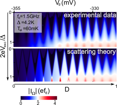
Figure 5: (color online). Contour plot of $\left|I_{\Omega}\right|$ as functions of the square excitation amplitude $2eV_{\mathrm{exc}}/\Delta$ (vertical scale) and the gate voltage $V_{g}$ or equivalently the QPC transmission $D$ (horizontal scale). Top panel: experimental results for sample $A$ from which we extract the parameters $\Delta=4.2K$, $f_{\mathrm{d}}=1.5$ GHz, and $T_{\mathrm{el}}\approx 60$ mK, see text. Bottom panel: numerical calculations based on Eq. (13) using the extracted model parameters.

We now consider actual experimental data: in Fig. 5a, we show experimental results for $|I_{\Omega}|$ as functions of the square excitation amplitude $V_{\mathrm{exc}}$ and the QPC gate voltage $V_{\mathrm{g}}$ (or correspondingly the QPC transparency $D$) taken from a sample that we label as sample $A$. The experiment was carried out in a dilution refrigerator and the driving frequency was $f_{d}=1.5$ GHz. The experimental results display a series of diamond-like structures centered around $2eV_{\mathrm{exc}}/\Delta=1$. The spacing of the diamonds at low gate voltages $V_{\mathrm{g}}$, where the QPC is nearly pinched off, allows us to extract the level spacing $\Delta=4.2$ K of the quantum dot. The electron temperature $T_{\mathrm{el}}\approx 60$ mK can moreover be determined from the smearing of the diamond structures. Finally, the capacitive coupling between the QPC gates and the quantum dot can be evaluated from the shift of the position of the levels as $V_{g}$ is varied. Using these parameters we evaluate numerically Eq. (13) as shown in Fig. 5 (bottom panel). To this end, we use a saddle-point transmission law for the QPCButtiker1990 . The agreement between the experimental data and numerical calculations is very good, up to small energy-dependent variations in the QPC transmission which were not included in the model.

Figure 5 allows us to locate operating regimes for which the mesoscopic capacitor is expected to function optimally as a controllable single electron source. The white areas of the diamonds correspond to plateaus on which the current $\left|I_{\Omega}\right|=2ef_{d}$ is given by the product of the driving frequency and twice the elementary charge $e$ (electrons and holes each contribute with an elementary charge, resulting in the factor of 2). In these regions, the device acts on average as a single electron source which emits in each cycle one single electron (hole) at a well defined energy far above (below) the Fermi level. The sharpness of the diamonds is then related to the accuracy of the expected quantization. Note that at low $V_{\mathrm{exc}}$ these regions become sharp peaks in $\left|I_{\Omega}\right|$ as a function of $V_{\mathrm{g}}$, corresponding to the HOL being resonant with the Fermi energy in absence of the driving ($\phi=0$) (in the linear regime $2eV_{\mathrm{exc}}\ll hf_{d},k_{B}T$, we also recover theoretically the known expression for the average AC current Buttiker1993 ; Gabelli2006 ). In contrast, the values of $V_{\mathrm{g}}$, where two diamonds intersect, interpolate at low $V_{\mathrm{exc}}$ to zeroes in the conductance corresponding to the Fermi energy lying midway in between two energy levels ($\phi=\pi$). For large transmissions, the quantization is gradually lost and the diamonds fade into a linear dependence of the current on the driving amplitude. For low transmissions on the other hand, the typical escape time of an electron on the quantum dot becomes much longer than the period, and charge emission becomes rare such that $I_{\Omega}$ is strongly suppressed.

In the strong driving regime $2eV_{\mathrm{exc}}\gg hf_{d}$, we recover theoretically well-known results for the average AC currentFeve2007 . In particular, a second-order expansion of Eq. (12) in the driving frequency, $\hbar\Omega=hf_{d}\ll D\Delta$, enables us to express $\langle\hat{I}(t)\rangle$ as the current response of an $RC$ circuit.Feve2007 Concretely, we find

$$\langle\hat{I}(t)\rangle=\sum_{k}\frac{iV_{\mathrm{exc}}}{\pi(2k+1)}\left(-i\Omega C_{q}+\Omega^{2}R_{q}C^{2}_{q}\right)e^{i(2k+1)\Omega t},$$ (22)

where

$$C_{q}=e^{2}\int d\epsilon\rho(\epsilon)\mathcal{F}(\epsilon,V_{\mathrm{exc}})$$ (23)

and

$$R_{q}=\frac{h}{2e^{2}}\frac{\int d\epsilon\rho^{2}(\epsilon)\mathcal{F}(\epsilon,V_{\mathrm{exc}})}{\left[\int d\epsilon\rho(\epsilon)\mathcal{F}(\epsilon,V_{\mathrm{exc}})\right]^{2}}.$$ (24)

are the $V_{\mathrm{exc}}$-dependent capacitance $C_{q}$ and resistance $R_{q}$, respectively, and we have defined the function

$$\mathcal{F}(\epsilon,V_{\mathrm{exc}})=\frac{f(\epsilon-eV_{\mathrm{exc}})-f(\epsilon+eV_{\mathrm{exc}})}{2eV_{\mathrm{exc}}}$$ (25)

in terms of the Fermi-Dirac distribution $f(\epsilon)$. We see that the capacitance $C_{q}$ is given by an integral of the density of states $\rho(\epsilon)$ over the energy window from $-eV_{\mathrm{exc}}$ to $+eV_{\mathrm{exc}}$. Under optimal operating conditions, where $\phi=0$, a peak in $\rho(\epsilon)$ is centered around $\epsilon=0$, such that the current becomes independent of $V_{\mathrm{exc}}$. This is clearly visible on the diamonds in Fig. 5.

In the following we restrict our considerations to excitation drives that exactly compensate the level spacing, i. e., $2eV_{\mathrm{exc}}=\Delta$. In this case, one of the peaks in $\rho(\epsilon)$ is always fully integrated over regardless of $\phi$, and the capacitance $C_{q}$ becomes independent of $\phi$ and $D$Feve2007 . In that case we obtain the simple result $C_{q}=e^{2}/\Delta$. For a square excitation drive voltage, the time-dependent average current is

$$\langle\hat{I}(t)\rangle=\frac{e}{\tau}\frac{e^{-t/\tau}}{1+e^{-T/2\tau}}$$ (26)

for $0\leq t\leq T/2$. Clearly, this is an exponentially decaying current with a characteristic $RC$ time given by the escape time $\tau=R_{q}C_{q}$, that is related to the QPC transmission $D$ as Buttiker2009

$$\tau\simeq\frac{h}{\Delta}\times\left(\frac{1}{D}-\frac{1}{2}\right)\simeq\frac{\tau_{o}}{D}\;,\,\quad D\ll 1,$$ (27)

where we recall that $\tau_{o}=h/\Delta$ is the time it takes an electron to complete one round inside the mesoscopic capacitor. Integrating next the current over one half-period of the driving we find the average transferred charge per half-period

$$Q^{t}=2V_{\mathrm{exc}}C_{q}\times\tanh(\frac{1}{4f_{d}\tau})=e\times\tanh(\frac{1}{4f_{d}\tau})\,.$$ (28)

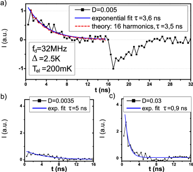
Figure 6: (color online). Time dependence of the average AC current $\langle\hat{I}(t)\rangle$ measured in sample $B$ for different values of the QPC transmission $D$. The level spacing and electron temperature of sample $B$ were $\Delta=2.5$ K and $T_{\mathrm{el}}\approx 200$ mK, respectively. The driving frequency was $f_{d}=32$ MHz. Experimental data is shown with symbols, while the blue lines are exponential fits from which the escape time $\tau$ is extracted. The green dashed line in panel a) corresponds to scattering theory calculations with 16 harmonics included. QPC transmission and extracted escape times are a) $D=0.005$, $\tau\approx 3.6$ ns, b) $D=0.0035$, $\tau\approx 5$ ns, and c) $D=0.03$, $\tau\approx 0.9$ ns.

The exponential decay of the current described by Eq. (26) was observed experimentally in Refs. Feve2007, and Mahe2008, . Typical experimental results are shown in Fig. 6 for a sample that we label as sample $B$Gabelli2006 ; Feve2007 ; Mahe2008 . For this sample, the level spacing was $\Delta=2.5$ K and the electron temperature $T_{\mathrm{el}}\approx 200$ mK, while the experiment was carried out at a driving frequency of $f_{d}=32$ MHz.

The current is well approximated by an exponential decay, allowing us to extract the escape time $\tau$, which is tunable by the QPC gate voltage $V_{g}$ and thus the QPC transparency $D$. For sufficiently large QPC transmissions, the integral of the current becomes constant (see also data in Ref. Mahe2008, ), demonstrating the quantization of the average transferred charge per half-period $Q^{t}=e$, so long as $f_{d}\tau\ll 1$ and thus $\tanh(\frac{1}{4f_{d}\tau})\simeq 1$ in Eq. (28). For low transmissions, $\langle\hat{I}(t)\rangle$ still exhibits an exponential decay with an escape time $\tau$ that is comparable to the half-period $T/2$. This indicates that the $RC$ circuit description of the single electron emitter is still valid even for $f_{d}\tau\simeq 1$. The $RC$ circuit description of the single electron emitter also allows us to extract $\tau=R_{q}C_{q}$ from measurements of the phase of the first harmonic $I_{\Omega}$ and $Q^{t}$ from both modulus and phase measurement of $I_{\Omega}$ for arbitrary values of the transmission $D$.

Using measurements of the modulus (see Figure 5) and phase of $I_{\Omega}$ for sample A, the $Q^{t}$ and $\tau$ dependence on the QPC gate voltage $V_{g}$ at excitation amplitude $2eV_{\mathrm{exc}}=\Delta$ are plotted in Fig. 7. As $V_{g}$ is swept from large negative voltages towards zero, the transmission $D$ increases, while the escape time $\tau$ decreases over two orders of magnitude. The blue line corresponds to the measurement data of $Q^{t}$ while the black dashed line expresses $Q^{t}$ in terms of $\tau$ according to Eq. (28). For sufficiently short escape times $\tau$, $Q^{t}$ becomes quantized and equal to the electron charge $e$ (corresponding to the quantization of the modulus of the first harmonic in units of $2ef$ in Fig. 5). Small residual oscillations around $Q^{t}=e$ stemming from the capacitive coupling between the QPC gates and the cavity can be seen. When $V_{g}$ is swept, the quantum dot goes periodically from optimal conditions $\phi=0$ ($\epsilon_{0}=0$) to $\phi=\pi$ ($\epsilon_{0}=\Delta/2)$. In the first case, $Q^{t}$ is quantized, i. e. $Q^{t}=e$, whereas in the second case, $Q^{t}$ becomes extremely sensitive to the exact value of the excitation amplitude and $Q^{t}\approx e$ (slightly above $e$ in Fig. 7) explaining the oscillations. The quantization of $Q^{t}$ can be checked on the inset of Fig. 7, showing $Q^{t}$ as a function of the escape time $\tau$ for conditions close to the optimal value of $\phi\approx 0$. For short escape times, all data agree with $Q^{t}=e$ within error bars (size of squares). In this regime, electrons and holes appear to be systematically emitted with the uncertainty in the emission time determined by $\tau$. In contrast, when the escape time becomes comparable to half a period, the expected quantization is lost, $Q^{t}<e$, reflecting that single charges are not deterministically and periodically emitted from the quantum dot. Furthermore, $Q^{t}/e$ (squares) is well described by the expected $\tanh{(1/4f_{d}\tau)}$ dependence (continuous black line). Finally, we note that the Floquet scattering matrix theory predicts rapid oscillations in the currentMoskalets2008 on time scales on the order of $\tau_{o}=h/\Delta$ which is much smaller than the periods considered here. The observation of such oscillations, however, is not yet within experimental reach, as the time scale $\tau_{o}\approx 10$ ps is still well below the measurement resolution of our experiment.

As we have seen in this section, the measurements of the average AC current suggest that the mesoscopic capacitor in certain parameter regimes acts as a controllable single electron source. Average measurements only, however, do not reveal possible fluctuations of the quantized current and to this end we need to consider the noise properties of the mesoscopic capacitor. As already discussed, the noise spectrum can be calculated numerically using the Floquet scattering matrix theory. In order to understand in detail the noise properties of the mesoscopic capacitor we first analyze a simple semi-classical model of the charge transport. The description of the mesoscopic capacitor in terms of an AC driven $RC$ circuit forms the basis of the semi-classical model described in the following section.

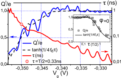
Figure 7: (color online). Measured average transferred charge per half-period $Q^{t}$ (blue line) and escape time $\tau$ (red line) for sample $A$ as functions of $V_{g}$. Parameters are $\Delta=4.2$ K, $T_{\mathrm{el}}\approx 60$ mK, and $f_{d}=1.5$ GHz. The dashed line corresponds to $Q^{t}$ determined from the measured $\tau$ using Eq. (28). The dotted circle corresponds to the point at which $\tau=T/2$. Inset: average transferred charge for optimal operating conditions ($\phi\approx 0$) as a function of the escape time $\tau$ in units of $T/2$.

V Semi-classical model

As mentioned above, the noise of the mesoscopic capacitor can be calculated numerically using the Floquet scattering theory. However, except for certain limiting cases, it is generally difficult to obtain analytic results from which one could hope to develop a deeper understanding of the noise properties. In the adiabatic regime, where the period of the driving is much longer than any other time scale, the noise spectrum has been found analyticallyMoskalets2002 ; Moskalets2007 ; Moskalets2008 . In contrast, in the situation that we consider here, where the driving potential is highly non-adiabatic, a perturbative expansion in the driving frequency is not possible. Nevertheless, both the experimental and the numerical results obtained from the Floquet scattering approach suggest that it may be possible to calculate analytically the noise spectrum using a conceptually simple semi-classical model. The model that we now describe was first suggested by Mahé et al.Mahe2010 and later investigated theoretically by Albert et al.Albert2010 . In the following we discuss the semi-classical model from which we derive the finite-frequency noise spectrum and provide a thorough comparison between analytic, numerical, and experimental results.

The semi-classical model can be explained by considering again Fig. 1b. The model assumes that the quantum dot can emit at most one electron and one hole per period and time is discretized in units of $\tau_{o}$; the time is takes an electron to complete one round inside the mesoscopic capacitor. In the emission phase \footnotesize{1}⃝ the probability in each time step for an electron to escape is equal to the transparency of the QPC, namely $D$. Additionally, since the amplitude of the periodic driving is on the order of the level spacing $\Delta$, higher-lying states can safely be neglected and maximally one electron can escape the mesoscopic capacitor as re-filling is not possible. Similarly, in the absorption phase \footnotesize{2}⃝ the probability of emitting a hole in each time step is $D$. This semi-classical model can be theoretically formulated as a master equation in discrete time for the probability of the mesoscopic capacitor to be occupied by an electron. Setting the electron charge $e=1$ in the following, this probability is equal to the average (additional) charge of the mesoscopic capacitor $\langle Q\rangle$, where $Q=0,1$.

The master equation determines the evolution of the average charge after one time step and takes the form Mahe2010 ; Albert2010

$$\langle Q(t_{k+1,\ell})\rangle=\left\{\begin{array}[]{ll}(1-D)\langle Q(t_{k,\ell})\rangle&\footnotesize{1}⃝\\ \\ D[1\!-\!\langle Q(t_{k,\ell})\rangle]\!+\!\langle Q(t_{k,\ell})\rangle&\footnotesize{2}⃝\end{array}\right.,$$ (29)

where we have used that $1-\langle Q\rangle$ is the probability for the mesoscopic capacitor to be empty and $t=t_{k,\ell}$ denotes time at the $k$’th time step during the $\ell$’th period. The emission (absorption) phase $\footnotesize{1}⃝$ ($\footnotesize{2}⃝$) corresponds to $k=1,2\ldots,K$ ($K+1,K+2,\ldots,2K$), where $K$ is the number of time steps in the absorption and emission phases, respectively, each of duration $T/2$.

Experimentally, the noise measurement frequency $\omega$ was roughly equal to the driving frequency $\Omega=2\pi f_{d}$ and both were much smaller than the inverse round trip time $\tau_{o}$, i. e. $2\pi/\omega\simeq 2\pi/\Omega\simeq 60\,\tau_{o}$ Mahe2010 . This allows us eventually to consider the continuous-time limit of the model, where the step size $\tau_{o}$ becomes irrelevant and drops out of the problem. Interestingly, the physics of the system is then governed by the single dimensionless ratio $T/\tau$ of the period $T$ over the escape (or correlation) time

$$\tau\equiv\frac{\tau_{o}}{\ln[1/(1-D)]}.$$ (30)

In the limit $D\ll 1$, we recover the expression in Eq. (27). At the end of this section, we discuss the physical meaning of the correlation time.

The master equation can be understood by considering the average current as it was calculated using Floquet scattering theory in Ref. Moskalets2008, . For the square-shaped driving considered in this work, the current consists of one step-like term with time step $\tau_{o}$ contained in an exponential envelope function and one oscillatory part with period $\tau_{o}$. The latter corresponds to the rapid oscillations of the current mentioned in the previous section. These oscillations are due to quantum interferences between different orbits in the mesoscopic capacitor and they vanish at high temperatures. Still, at arbitrary temperature only the first step-like term survives after integration over the time step $\tau_{o}$, which leads to the master equation. The semi-classical description reflects that the oscillations due to quantum interferences are irrelevant for the average current on a time scale that is larger than $\tau_{o}$.

At this point we have not provided a detailed derivation of the model which would require us to compare not only average current but also noise and higher-order correlations with the full quantum theory. This still remains a challenging and open task and for now we simply rely on the excellent agreement with experimental data as we demonstrate in the following. Obviously, the semi-classical description cannot be correct under all operating conditions and already now we can anticipate situations where the model will differ from the full Floquet scattering theory: for example, as the noise measurement frequency approaches the internal frequency of the quantum dot, namely the frequency $h/\Delta=1/\tau_{o}$ associated with the level spacing $\Delta$, we expect that the semi-classical model will no longer be valid. The model also neglects the possibility of emitting two electrons within the same period and will therefore not apply to situations, where a level of the quantum dot is in resonance with the Fermi level of the 2D electron gas, i. e. for $\phi=\pi$. We make a detailed comparison between the semi-classical model and numerics in the following section.

Before turning to calculations of the noise spectrum, we consider the average charge $\langle Q\rangle$ in the mesoscopic capacitor. In Ref. Albert2010, the average charge was used to obtain the average current flowing out of the mesoscopic capacitor $\langle I(t)\rangle\equiv-\langle\dot{Q}(t)\rangle\simeq[\langle Q(t)\rangle-\langle Q(t+\tau_{o})\rangle]/\tau_{o}$. Solving Eq. (29) for the average charge $\langle Q\rangle$ we readily find

$$\langle Q(t_{k,\ell})\rangle=\left\{\begin{array}[]{ll}\displaystyle\alpha_{\ell}\,e^{-(t_{k,\ell}-\ell T)/\tau}&\footnotesize{1}⃝\\ \\ \displaystyle 1-\beta_{\ell}\,e^{-(t_{k,\ell}-[\ell+\frac{1}{2}]T)/\tau}&\footnotesize{2}⃝\end{array}\right..$$ (31)

Here, we have defined $\varepsilon=e^{-T/2\tau}$, $\alpha_{\ell}=1/(1+\varepsilon)+\theta\varepsilon^{2\ell}$ and $\beta_{\ell}=1/(1+\varepsilon)-\theta\varepsilon^{2\ell-1}$ with $\theta$ depending on the initial conditions at the time when the periodic driving is turned on. The correlation time $\tau$ determines the time scale over which the system loses memory about the initial conditions encoded in $\theta$ and $\langle Q\rangle$ becomes periodic in time. We notice the close relation of the above expression with the average current of an $RC$ circuit. Importantly, the model reproduces the expressions in Eqs. (26) and (28) for the time-dependent average current and the average transferred charge per half-period, respectively, obtained from the Floquet scattering theory.

VI Noise spectrum

We are now ready to discuss the noise properties of the mesoscopic capacitor. As we will see, the finite-frequency noise spectrum allows us to characterize the mesoscopic capacitor as a single electron source as well as to determine the optimal operating conditions of the device. Before presenting any detailed calculations we discuss the two primary sources of noise.

VI.1 Sources of noise

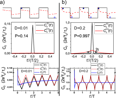
Figure 8: (color online). Current correlators within the semi-classical description. a) Shot noise limit: for small escape probabilities $D$, charges are not systematically emitted within each half-period: the emission probability per half-period $P=Q^{t}/e$ is small, and the current fluctuations correlator is essentially given by the Dirac peak in $C_{0}^{\langle II\rangle}(t^{\prime})$. The correlators $C_{0}^{\langle II\rangle}(t^{\prime})$, $C_{0}^{\langle I\rangle\langle I\rangle}(t^{\prime})$ and $C_{0}(t^{\prime})$ for long time $t^{\prime}$ are shown in the lower panel (with black, red, and blue lines, respectively): $C_{0}(t^{\prime})$ is negative for $t^{\prime}\lesssim 3T$, reflecting the anti-bunching of emitted charges. b) Phase noise limit: for sufficiently large escape probabilities (here, $D=0.2$), charges are systematically emitted ($P\simeq 1$), and $C_{0}^{\langle I\rangle\langle I\rangle}(t^{\prime})$ consists of a peak with a finite width given by the escape time $\tau$. In this case, $C_{0}(t^{\prime})$ is negative in a smaller range of times $t^{\prime}\lesssim T/2$.

In the semi-classical model, the mesoscopic capacitor emits at most one electron and one hole per period. Still, depending on the ratio between the escape time $\tau$ and the period $T$, the source may fail to emit. We quantify the emission probability per half-period by the ratio

$$P=Q^{t}/e,$$ (32)

having recalled that $Q^{t}$ is the average transferred charge per cycle, see Eq. (28). We refer to the noise associated with such cycle missing events, where the mesoscopic capacitor fails to emit, as shot noise. However, even when the emission probability is close to unity and the mesoscopic capacitor emits an electron and a hole in almost every cycle, there are still fluctuations in the current associated with the random emission times within a period. This source of noise is referred to as phase noise. The two uppermost panels of Fig. 8 illustrate the main sources of noise by showing typical realizations of the current, where emissions of electrons (holes) are shown with filled (empty) circles, on top of the average current. The uppermost panel of Fig. 8a illustrates shot noise, while the uppermost panel of Fig. 8b corresponds to phase noise.

From the definition of the current-current correlation function in Eq. (14) we can immediately write

$$C(t,t^{\prime})=\langle I(t)I(t+t^{\prime})\rangle-\langle I(t)\rangle\langle I(t+t^{\prime})\rangle,$$ (33)

where $I(t)$ is no longer a quantum mechanical operator, since we are considering a semi-classical description. As already mentioned, the system is not translational invariant in time due to the periodic gate voltage modulations. The correlation function therefore does not only depend on the time difference $t^{\prime}$, but also on the absolute time $t$. Experimentally, the correlation function is averaged over the absolute time $t$ and the time-average correlation function is then

$$C_{0}(t^{\prime})=C_{0}^{\langle II\rangle}(t^{\prime})-C_{0}^{\langle I\rangle\langle I\rangle}(t^{\prime}),$$ (34)

where $C_{0}^{\langle II\rangle}(t^{\prime})=\overline{\langle I(t)I(t+t^{\prime})\rangle}^{\,t}$ and $C_{0}^{\langle I\rangle\langle I\rangle}(t^{\prime})=\overline{\langle I(t)\rangle\langle I(t+t^{\prime})\rangle}^{\,t}$. The time-average correlation function is exactly the Fourier component $C_{0}(t^{\prime})$ entering Eq. (15) and the corresponding noise spectrum is consequently given by Eq. (16).

Figure 8 shows numerical calculations of the correlation functions in the two limiting cases. The results were obtained in numerical simulations of the stochastic process defined by the semi-classical model. The left panels correspond to the shot noise regime, where the escape time $\tau$ is much larger than the period $T$, whereas the right panels show results for the phase noise regime. Depending on the escape probability $D$ [or equivalently the ratio between the escape time and the period, see Eq. (30)], the contributions from $C_{0}^{\langle II\rangle}(t^{\prime})$ and $C_{0}^{\langle I\rangle\langle I\rangle}(t^{\prime})$ vary. The two central panels of Fig. 8 show the correlation functions $C_{0}^{\langle II\rangle}(t^{\prime})$ and $C_{0}^{\langle I\rangle\langle I\rangle}(t^{\prime})$ for short times $t^{\prime}\ll T$. In both regimes, $C_{0}^{\langle II\rangle}(t^{\prime})$ contains a Dirac peak at $t^{\prime}=0$. Indeed, since maximally one charge is emitted per half-period, the short-time correlations vanish. In this respect, the Dirac peak is the hallmark of single particle emission. Correlations are only recovered when $t^{\prime}$ is close to a multiple of the half-period, as seen in the lower panels of Fig. 8.

The height of the Dirac peak at $t^{\prime}=0$ is proportional to the average transferred charge per half-period $Q^{t}$: $C_{0}^{\langle II\rangle}(t^{\prime}=0)$ counts the average number of peaks and dips in the instantaneous current $I(t)$ corresponding to emitted electrons and holes. The correlation function $C_{0}^{\langle I\rangle\langle I\rangle}(t^{\prime})$ is given by the autocorrelation of the exponentially decaying average current. At short times, it therefore has a peak at $t^{\prime}=0$ with a finite width given by the escape time $\tau$. At times comparable to multiples of half a period, correlations are again recovered, which compensate the long-times correlations in $C_{0}^{\langle II\rangle}(t^{\prime})$. Thus, for long times $t^{\prime}\gg T$, the correlation function $C(t^{\prime})$ vanishes since charges emitted by the source are no longer correlated. The timescale on which $C(t^{\prime})$ decays to zero depends on the transmission $D$ and is given by the escape (or correlation) time $\tau$.

VI.1.1 Shot noise

For small escape probabilities $D\ll 1$, the escape time $\tau$ becomes much larger than the period $T$. The peak at $t^{\prime}=0$ in $C_{0}^{\langle I\rangle\langle I\rangle}(t^{\prime})$ correspondingly becomes much smaller than the Dirac peak in $C_{0}^{\langle II\rangle}(t^{\prime})$, see Fig. 8a. The current correlator $C(t^{\prime})$ is thus given by a Dirac peak at $t^{\prime}=0$ combined with negative values up to at finite times on the order of the correlation time $\tau$. The noise power spectral density is then constant, except at zero frequency, where it vanishes because the integrals over $C_{0}^{\langle II\rangle}(t^{\prime})$ and $C_{0}^{\langle I\rangle\langle I\rangle}(t^{\prime})$ cancel each other. In this case, the source randomly emits charges and the charge fluctuations are similar to shot noise.

The negative values of $C(t^{\prime})$ at finite times reflect the anti-bunching behavior of emitted charges: at low transmission probabilities $D$, the anti-bunching extends over a large range of times, $t^{\prime}\simeq\tau$, see Fig. 8a (lower panel). Even in the shot noise regime, a hole must be emitted after the emission of an electron before a second electron can be emitted. Now, approximating $C_{0}^{\langle I\rangle\langle I\rangle}(t^{\prime})\simeq 0$, see Fig. 8a, and writing $C_{0}^{\langle II\rangle}(t^{\prime})=(2f_{d}Q^{t}/e)\delta(t^{\prime})$, we findMahe2010 ; Albert2010

$$S_{\rm shot}(\omega)=4e^{2}f_{d}\times P=\frac{e^{2}}{\tau},$$ (35)

where $P$ the emission probability per half-period, Eq. (32). Interestingly, this expression is identical to the usual shot noise formula $S=2eI_{p}$, where the usual charge current has to be replaced by the particle current, $I_{p}$, given by the sum of the average number of electrons emitted in the first half period and holes in the second one, times the product of the electric charge with the drive frequency: $I_{p}=2ef_{d}\times P$.

VI.1.2 Phase noise

In the phase noise regime, the escape probability $D$ is so high that charges are emitted in nearly every cycle and the emission probability $P$ is close to unity. The time-dependent average current then consists of well-defined exponential decays with a decay time given by the escape time $\tau\ll T/2$: $\langle I(t)\rangle=\pm(e/\tau)e^{-t/\tau}$. Here the different signs correspond to the emission of electrons or holes. In this case, we find a simple expression for the correlation function

$$C_{0}^{\langle I\rangle\langle I\rangle}(t^{\prime})=\frac{e^{2}f_{d}}{\tau}e^{-|t^{\prime}|/\tau}\,.$$ (36)

and the noise is then given byMahe2010 ; Albert2010

$$S_{\rm phase}(\omega)=4e^{2}f_{d}\frac{\omega^{2}\tau^{2}}{1+\omega^{2}\tau^{2}}\,.$$ (37)

Even if charges are systematically emitted each period, we find a finite value of the noise which depends only on the escape time $\tau$. This noise is due to the uncertainty in the emission time of charges within a period, and is thus referred to as phase noise. The phase noise is an intrinsically high-frequency noise and it is the signature of single charge emission: when the source periodically emits single charges, the noise reduces to the value of the phase noise determined only by the temporal extension $\tau$ of the emitted wave packets.

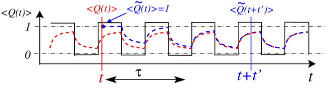
Figure 9: (color online). Schematics of periodic driving and (conditional) charge occupations. The mean occupation of the mesoscopic capacitor $\langle Q(t)\rangle$ is shown in red. The mean occupation is equal to the probability of the mesoscopic capacitor to be occupied with one (additional) electron. The blue curve shows the conditional mean occupation $\langle\widetilde{Q}(t+t^{\prime})\rangle$. This is the probability that the mesoscopic capacitor is charged with an (additional) electron at time $t+t^{\prime}$, given that it was charged at time $t$, such that $\langle\widetilde{Q}(t)\rangle=1$. Correlations decay on a time scale set by the correlation time $\tau$, implying that $\langle\widetilde{Q}(t+t^{\prime})\rangle\simeq\langle Q(t+t^{\prime})\rangle$ for $t^{\prime}\gg\tau$.

VI.2 Analytic expression

We now present an analytic calculation of the noise power spectrum which covers both limiting cases as well as the intermediate regime Albert2010 . To this end, it is useful to consider the charge correlation function $C_{Q}(t,t^{\prime})=\langle Q(t)Q(t^{\prime})\rangle-\langle Q(t)\rangle\langle Q(t^{\prime})\rangle$ together with the relation $\mathcal{P}_{0}(\omega)\simeq\omega^{2}\mathcal{P}_{Q}(\omega)$. Here the definition of $\mathcal{P}_{Q}(\omega)$ is similar to that of $\mathcal{P}_{0}(\omega)$ in Eq. (16), but with the current $I$ replaced by the charge $Q$. The charge correlation function can be evaluated following the schematic illustration in Fig. 9. We first note that $\langle Q(t)Q(t+t^{\prime})\rangle$ is the joint probability for the capacitor to be charged with one electron both at time $t$ and at time $t+t^{\prime}$. Using conditional probabilities we then write $\langle Q(t)Q(t+t^{\prime})\rangle=\langle Q(t)\rangle\langle\widetilde{Q}(t+t^{\prime})\rangle$, where $\langle\widetilde{Q}(t+t^{\prime})\rangle$ is the probability that the capacitor is charged with one electron at time $t+t^{\prime}$ given that it is charged at time $t$. For $t^{\prime}>0$, the conditional probability $\langle\widetilde{Q}(t+t^{\prime})\rangle$ can be found by propagating forward in time the condition $\langle\widetilde{Q}(t)\rangle=1$ using the master equation in Eq. (29), see also Fig. 9. Similar reasoning applies to the case $t^{\prime}<0$. Finally, integrating over $t$, the time-averaged charge correlation function becomes $\overline{\langle\delta Q(t)\delta Q(t+t^{\prime})\rangle}^{\,t}=\,\frac{\tau}{T}\,e^{-|t^{\prime}|/\tau}\tanh\left(\frac{T}{4\tau}\right)$, and we immediately obtain the noise power spectrum as Albert2010

$$S(\omega)=4e^{2}f_{d}\;\tanh\left(\frac{1}{4f_{d}\tau}\right)\,\frac{\omega^{2}\tau^{2}}{1+\omega^{2}\tau^{2}}\,.$$ (38)

Interestingly, the noise power spectrum is given by the average charge emitted during the emission phase $\tanh(1/4f_{d}\tau)$ (the factor of 2 accounts for the additional contribution from the average charge absorbed in the absorption phase) multiplied by a Lorentzian-like frequency dependence, which accounts for the exponential decay of correlations in the time domain with time constant $\tau$. Finally, the factor $\omega^{2}\tau^{2}$ reflects that the noise spectrum becomes flat in the high-frequency limit, while the zero-frequency limit $S(0)=0$ shows that charge on average does not accumulate on the capacitor once $\langle Q\rangle$ has become periodic in time. From Eq. (38) it is straightforward to recover the limiting cases given by Eqs. (35) and (37), but the analytic result above also accounts for the intermediate regime where the escape time $\tau$ is comparable to the period $T$.

VI.3 Detailed comparison

We are now ready to carry out a careful comparison of experimental and theoretical results. In Fig. 10 we first compare results for the noise spectrum obtained from the full Floquet scattering theory and the semi-classical model. We focus here on the experimentally relevant regime with $\omega\approx\Omega\ll\Delta/\hbar$ together with the optimal operating conditions of the source, $\phi=0$, and consider three different values of the transmission probability $D$. The figure shows that the two complementary approaches yield results that are in excellent agreement. We observe that our numerical and analytic calculations agree well both in the shot noise limit with $D=0.01$ ($\tau\approx 3.5\>T/2$) and in the phase noise limit with $D=0.2$ ($\tau\approx 0.16\>T/2$), as well as in the intermediate cross-over regime. For $\omega\tau\gg 1$, the phase noise $S_{\rm phase}$ saturates to $4e^{2}f_{d}$, such that $S(\omega)\simeq 4e^{2}f_{d}P$ as seen both for $D=0.06$ ($\tau\approx 0.57\>T/2$, $P=0.71$) and $D=0.01$ ($P=0.14$).

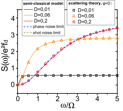
Figure 10: (color online). Finite-frequency noise $S(\omega)$ close to the driving frequency, $\omega\sim\Omega$. Symbols: scattering theory ($\phi=0$); continuous lines: semi-classical model; dashed lines: limits given by Eqs. (35) and (37). Parameters are $\Delta=4K$ and $f_{d}=1.5$ GHz.

The two theoretical approaches can also be compared with experimental data, obtained with sample A using a high sensitivity microwave noise measurement setup implemented in a dilution refrigerator Parmentier2011 . The noise was measured in a bandwidth of $1.2-1.8$ GHz centered around the driving frequency $f_{d}=1.5$ GHz. Figure 11 shows the dependence of the noise $S(\omega=\Omega)$ on the escape time $\tau$. The numerical and analytic results (overlapping continuous lines) are in excellent agreement with the experimental data (circles) obtained at $\phi\approx 0$. In particular, the experimental results are captured by the analytical expression in Eq. (38) over more than two orders of magnitude of the escape time $\tau$, going from the phase noise limit (blue dashed line), where the source exactly emits a single electron and a single hole in each cycle, to the shot noise limit (black dashed line) where particle emissions are rare and shot noise likeAlbert2010 . As discussed in Sec. IV, the average emission probability $P$ (squares) is also well captured by the expected $\tanh{1/4f_{d}\tau}$ dependence (continuous black line). The results shown in Fig. 11 demonstrate that the mesoscopic capacitor indeed behaves as an controllable on-demand single electron emitter when operated under optimal conditions.

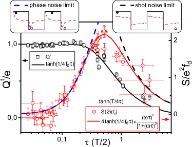
Figure 11: (color online). Noise power spectrum $S(\omega=\Omega)$ as a function of the escape time $\tau$. Left axis: measured average transferred charge per half-period $Q^{t}$ (black squares) together with Eq. (28) (continuous black line). Right axis: measured noise spectrum (red circles, $\phi\approx 0$, sample A) together with Eq. (38) (red line). Dashed lines correspond to the two noise limits, Eqs. (35) and (37), illustrated schematically in the top panels.

VI.4 Universality and deviations

While the semi-classical model is only valid for a restricted range of parameters, the Floquet scattering theory in contrast allows us to explore the full set of experimentally relevant operating conditions, including changes of temperature, level spacing, and measurement frequency $\omega/2\pi$. In the following, we first discuss a particular universal property of the noise under optimal operating conditions as described by the semi-classical model. Secondly, we discuss possible discrepancies between the semi-classical model and the full numerical calculations based on the Floquet scattering theory. As we will see below, the two descriptions start to differ once the system is not operated under optimal conditions, or when the noise is measured at very large frequencies $\hbar\omega\sim\Delta$.

VI.4.1 Universality

Figure 10 clearly illustrates that the Floquet scattering theory and the semi-classical model agree well under optimal operating conditions. Moreover, by plotting the noise power $S(\omega=\Omega)$ in units of the driving frequency $e^{2}f_{d}$ as a function of the escape time $\tau$ in units of the half-period $T/2$ one finds strong indications of a simple universal behavior of the noise power which is independent of the specific parameters of the system. Indeed, by rewriting Eq. (38) in term of these normalized units, we find

$$S(\Omega)_{[e^{2}f_{d}]}=4\tanh\left(\frac{1}{2\tau_{[T/2]}}\right)\,\frac{(\pi\tau_{[T/2]})^{2}}{1+(\pi\tau_{[T/2]})^{2}},$$ (39)

from which this universality is evident. In particular, neither the level spacing $\Delta$ nor the temperature enter this expression. The universality of the noise spectrum is verified by our full numerical Floquet scattering theory calculations with different values of $\Delta$ as shown in Fig. 12 (the dependence of $\tau$ on $\Delta$ is taken into account). We also checked performed calculations with varying temperatures (not shown) and found good agreement with the expression above. The universal behavior can be understood by noting that under optimal operating conditions, the noise arises from elementary charge transfer processes which only depend on the parameter $\tau$. As long as the charges are emitted sufficiently far above or below the Fermi level, these processes do not depend of the energy at which the charges are emitted.

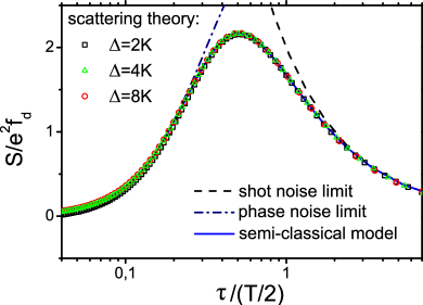
Figure 12: (color online). Universality of the noise spectrum. Noise spectrum based on the semiclassical model, Eq. (39) (blue line), and full numerical Floquet scattering theory for different values of the level spacing (symbols) as a function of the escape time $\tau$ with $T_{\rm el}=100$ mK. The dashed lines correspond to the two limits given by Eqs. (35) and (37).

VI.4.2 Deviations

Deviations from the universal behavior start to appear as the QPC transmission approaches unity, $D\simeq 1$, and the escape time $\tau$ becomes comparable to the inverse level spacing $\tau_{o}=h/\Delta$. For short escape times, Eq. (39) predicts that the noise would vanish. However, the semi-classical description is expected to break down as the relevant time scales of the problem approach $\tau_{o}$. Small deviations between the semi-classical model and full numerics are already visible in Fig. 12 for $\tau\lesssim 0.1\>T/2$. The semi-classical model is also not expected to be valid when one of the levels in the quantum dot is brought into resonance with the Fermi energy during the emission cycle. In this case, the total charge on the quantum dot is no longer quantized and the quantization of the first harmonics of the average AC current is lost, see Fig. 5. Under these conditions, the noise is expected to depend strongly on various parameters such as temperature, the shape of the excitation drive, and the static potential in the quantum dot.

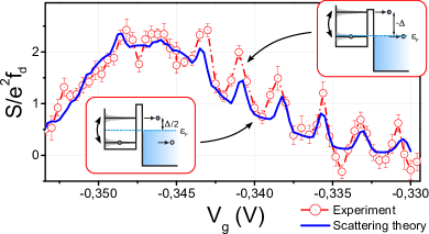
Figure 13: (color online). Noise spectrum as a function of the QPC gate voltage $V_{g}$. Circles: experimental data (sample $A$); continuous line: Floquet scattering theory ($\Delta=4$ K, $T_{\rm el}=100$ mK, 3 odd harmonics in the excitation drive). The panels illustrate charge emission in the minima ($\phi=0$) and the maxima ($\phi=\pi$) of the noise oscillations.

The expected parameter dependencies are clearly visible in the noise measurements. In Fig. 13 we show the measured noise spectrum as a function of the QPC gate voltage $V_{g}$ (red circles), which simultaneously controls the QPC transmission $D$ and the levels in the quantum dot via a capacitive coupling, see also Fig. 5. Oscillations in the noise are observed for $-0.345$ V $\lesssim V_{g}\lesssim$ $-0.330$ V (0.8 $\lesssim P\lesssim 1$). The maxima of the oscillations correspond to the case $\phi=\pi$, where one of the levels is brought into resonance with the Fermi energy, while the minima occur at the optimal operating conditions $\phi=0$, see insets in Fig. 13. The semi-classical model cannot account for these oscillationsMahe2010 . Instead, we have used the Floquet scattering theory and numerically evaluated Eq. (21) as a function of $V_{g}$. The dependence of the QPC transmission on the gate voltage $D(V_{g})$ was extracted using Eq. (27) in combination with the escape time $\tau$ as a function of $V_{g}$, Fig. 7. The AC drive $V_{\rm exc}(t)$ used in the calculations consisted of three odd harmonics, accounting for the finite bandwidth of the microwave pulse generator used in the experiments.

The numerical results (blue line) shown in Fig. 13 are in good agreement with the experimental data. The maxima in the noise can be understood by noting that a square-shaped AC drive with a finite number of harmonics contains fast oscillations, or ripples, which affect the energy resolution of the emitted charges. In the case $\phi=\pi$, the level brought into resonance with the Fermi energy and then oscillates rapidly with respect to the Fermi energy. This “shaking” of a resonant level causes additional charge transfers (which also depend on the QPC transmission), leading to an increase in the noise. Due to such spurious emissions of electron–hole pairs, the source does not behave as a perfect single particle emitter under these operating conditions.

Deviations between the Floquet scattering theory and the semi-classical model also occur when the measurement frequency becomes comparable to the level spacing $\omega\simeq\Delta/\hbar$. Indeed, since the semi-classical model describes the dynamics of charge emissions with a discrete time step $\tau_{o}=h/\Delta$, it cannot account for dynamics on time scales shorter than $\tau$, or large measurement frequencies $\omega\simeq\Delta/\hbar$. The Floquet scattering model, on the other hand, predicts fast oscillations on time scales comparable to $\tau_{o}$ in the average AC currentMoskalets2008 . We therefore expect strong deviations between the semi-classical model and the Floquet scattering theory in the noise spectrum at high frequencies.

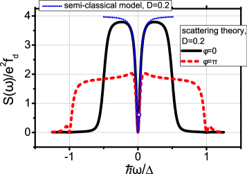
Figure 14: (color online). Noise spectrum as a function of the measurement frequency $\omega$. Blue dotted line: semi-classical model. Since time is discretized in units of $\tau_{o}=h/\Delta$, $S(\omega)$ can only be calculated up to $\hbar\omega=\Delta/2$. Black line: Floquet scattering theory with $\phi=0$. Red dashed line: Floquet scattering model with $\phi=\pi$. The electronic temperature was set to $T_{\rm el}=100$ mK. The blue circle denotes the noise at the driving frequency, $\omega=\Omega$. Parameters are $D=0.2$ ($P\approx 1$), $\Delta=4$ K, and $f_{d}=1.5$ GHz.

Numerical calculation of the noise spectrum at high measurement frequencies are shown in Fig. 14 obtained from the Floquet scattering theory and the semi-classical model. We see that the two complementary approaches agree well at small frequencies for $\phi=0$. However, while the noise in the semi-classical model saturates to $S(\omega\gg\Omega)=4e^{2}f_{d}$ at high frequencies, the Floquet scattering theory, in contrast, is cut off for $\hbar\omega\approx\Delta/2$, where it drops to zero. Indeed, the electrons (holes) are emitted at an energy $\Delta/2$ above (below) the Fermi energy, corresponding to emission of radiation (or photons) at frequencies below $\Delta/2$. For $\phi=\pi$, charges can be emitted at energies up to $\Delta$ above or below the Fermi energy, and the cutoff frequency is then equal to $\Delta$ as seen in the figure. We note that the excess noise shown here indeed is symmetric in $\omega$ as expected.

VI.5 Full counting statistics

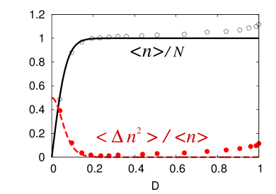
Figure 15: (color online). Mean and variance of the counting statistics of emitted electrons $P(n,N)$ after a large number of periods $N$ as functions of the QPC transparency $D$. Full lines: Results based on the semi-classical model. Symbols: Numerical data obtained from the Floquet scattering theory. Numerical results (symbols) were adapted from Ref. Gre10, .

We round off this section by discussing the counting statistics of emitted electrons. Under optimal operating conditions, the semi-classical model fully accounts for the charge dynamics of the emitter at low frequencies and it allows for tractable calculations of the counting statistics $P(n,N)$ of the number of emitted electrons $n$ during a large number of periods. In principle, we can calculate all moments (or cumulants) of the distributionAlbert2010 ; Pistolesi2004 ; Battista2011 , but we focus here on the first and second cumulant, the mean $\langle n\rangle$ and the variance $\langle\Delta n^{2}\rangle$ with $\Delta n=n-\langle n\rangle$. In Fig. 15 we show a comparison between the calculations of the first two cumulants based on the semi-classical modelAlbert2010 and Floquet scattering theoryGre10 . We observe an excellent agreement for small transparencies, but eventually deviations appear for $D\gtrsim 0.3$. These discrepancies appear as the broadening of energy levels become so large that the effect of spurious emissions of (several) electron-hole pairs during a period becomes non-negligible. In this case, the mean number of emitted electrons during a period can exceed one. The counting statistics is important for characterizing the accuracy of the mesoscopic capacitor as a single electron emitterAlbert2010 .

VII Conclusions

We have investigated experimentally and theoretically the finite-frequency noise spectrum of the mesoscopic capacitor when operated as a periodic single electron emitter. We have compared experimental data with two complementary theoretical descriptions. On one hand, we discussed the Floquet scattering theory which allows us to accurately describe the system over the full range of experimentally relevant parameters, in particular the energy ranges in which charges are emitted. On the other hand, we considered a semi-classical model which, despite its simplicity, is able to account for the charge dynamics of the emitter when operated under the optimal operating conditions. This model allowed us to develop an analytic understanding of the measured noise spectrum and the numerical results obtained using the Floquet scattering theory.

Depending on the escape time of electrons from the mesoscopic capacitor, two distinct noise regimes could be identified. When the escape time is much smaller than the period of the drive, the mesoscopic capacitor emits electrons and holes in an almost fully periodic manner with unit probability and the main source of noise is due to the uncertainty in the emission time within a period. This type of noise, referred to as phase noise, can be clearly identified both in the theoretical and experimental results. The phase noise provides a fundamental lower limit on the noise, arising from the random jitter between the triggering of emission and the actual emission time. In the phase noise regime, we obtained excellent agreement between our experimental data, the Floquet scattering theory, and the semi-classical model. In the other extreme, when the escape time of electrons is much larger than the period of the drive, electron emission becomes rare and the fluctuations are shot noise-like with a white spectrum related to the average (particle) current $I_{p}=2ef_{d}\times P$ through the usual Schottky formula $S_{\mathrm{Schottky}}=2eI_{p}$.

As the mesoscopic capacitor is tuned away from the optimal operating conditions and charges are emitted close to the Fermi energy, a significant increase in the noise is observed due to additional charge fluctuations generated by the source. These spurious emission processes are not accounted for by the semi-classical model, in which maximally one electron–hole pair can be emitted during each cycle. In contrast, these additional fluctuations are fully accounted for by the Floquet scattering theory. The ability to accurately investigate, model, and characterize the single electron emission process will prove useful in future few electron experiments involving the mesoscopic capacitor as a controllable single electron source.

- (1) Y. Ji, Y. Chung, D. Sprinzak, M. Heiblum, D. Mahalu, and H. Shtrikman, Nature 422, 415 (2003).
- (2) L. V. Litvin, H.-P. Tranitz, W. Wegscheider, and C. Strunk, Phys. Rev. B 75, 033315 (2007).
- (3) P. Roulleau, F. Portier, and P. Roche, Phys. Rev. Lett. 100, 126802 (2008).
- (4) I. Neder, N. Ofek, Y. Chung, M. Heiblum, D. Mahalu, and V. Umansky, Nature 448, 333 (2007).
- (5) P. Samuelsson, E. V. Sukhorukov, and M. Büttiker, Phys. Rev. Lett. 92, 026805 (2004).
- (6) P. Samuelsson, I. Neder, and M. Büttiker, Phys. Scripta T137, 014023 (2009).
- (7) G. Fève, A. Mahé, J.-M. Berroir, T. Kontos, B. Plaçais, A. Cavanna, B. Etienne, Y. Jin, and D.C. Glattli, Science 316, 1169 (2007).
- (8) M. D. Blumenthal, B. Kaestner, L. Li, S. Giblin, T. J. B. M. Janssen, M. Pepper, D. Anderson, G. Jones, and D. A. Ritchie, Nature Phys. 3, 343 (2007).
- (9) J. P. Pekola, J. J. Vartiainen, M. Möttönen, O.-P. Saira, M. Meschke, and D. V. Averin, Nature Phys. 4, 120 (2008).
- (10) F. Giazotto, P. Spathis, S. Roddaro, S. Biswas, F. Taddei, M. Governale, and L. Sorba, Nature Phys. 7, 857 (2011).
- (11) C. Leicht, P. Mirovsky, B. Kaestner, F. Hohls, V. Kashcheyevs, E. V. Kurganova, U. Zeitler, T. Weimann, K. Pierz, and H. W. Schumacher Semicond. Sci. Tech. 26, 055010 (2011).
- (12) S. Hermelin, S. Takada, M. Yamamoto, S. Tarucha, A. D. Wieck, L. Saminadayar, C. Bäuerle, and T. Meunier, Nature 477, 435 (2011).
- (13) R. P. G. McNeil, M. Kataoka, C. J. B. Ford, C. H. W. Barnes, D. Anderson, G. A. C. Jones, I. Farrer, and D. A. Ritchie, Nature 477, 439 (2011).
- (14) M. Büttiker, H. Thomas, and A. Prêtre, Phys. Lett. A 180, 364369 (1993).
- (15) S. E. Nigg, R. López, and M. Büttiker, Phys. Rev. Lett. 97, 206804 (2006).
- (16) M. Büttiker and S. E. Nigg, Nanotechn. 18, 044029 (2007).
- (17) Z. Ringel, Y. Imry, and O. Entin-Wohlman, Phys. Rev. B 78, 165304 (2008).
- (18) C. Mora and K. Le Hur, Nature Phys. 6, 697 (2010).
- (19) Y. Hamamoto, T. Jonckheere, T. Kato, and T. Martin, Phys. Rev. B 81, 153305 (2010).
- (20) J. Splettstoesser, M. Governale, J. König, and M. Bü ttiker, Phys. Rev. B 81, 165318 (2010).
- (21) M. Filippone, K. Le Hur, and C. Mora, Phys. Rev. Lett. 107, 176601 (2011).
- (22) M. Lee, R. López, M.-S. Choi, T. Jonckheere, and T. Martin, Phys. Rev. B 83, 201304(R) (2011).
- (23) J. Gabelli, G. Fève, J.-M. Berroir, B. Plaçais, A. Cavanna, B. Etienne, Y. Jin, and D.C. Glattli, Science 313, 499 (2006).
- (24) S. Ol’khovskaya, J. Splettstoesser, M. Moskalets, and M. Büttiker, Phys. Rev. Lett. 101, 166802 (2008).
- (25) S. Juergens, J. Splettstoesser, and M. Moskalets, Europhys. Lett. 96, 37011 (2011).
- (26) J. Splettstoesser, M. Moskalets, and M. Büttiker, Phys. Rev. Lett. 103, 076804 (2009).
- (27) C. Grenier, R. Hervé, E. Bocquillon, F. D. Parmentier, B. Plaçais, J. M. Berroir, G. Fève, and P. Degiovanni, New J. Phys. 13, 093007 (2011).
- (28) C. Grenier, PhD Thesis, Ecole Normale Supérieure de Lyon, http://tel.archives-ouvertes.fr/tel-00617869 (2011).
- (29) P. Degiovanni, C. Grenier, and G. Fève, Phys. Rev. B 80, 241307 (R) (2009).
- (30) G. Haack, M. Moskalets, J. Splettstoesser, and M. Büttiker, Phys. Rev. B 84, 081303 (R) (2011).
- (31) L. S. Levitov and G. B. Lesovik, JETP Lett. 58, 230 (1993).
- (32) Yu. V. Nazarov (ed.), Quantum Noise in Mesoscopic Physics (NATO Science Series, Kluwer, Dordrecht, 2003).
- (33) M. Albert, C. Flindt, and M. Büttiker, Phys. Rev. Lett. 107, 086805 (2011).
- (34) A. Mahé, F. D. Parmentier, E. Bocquillon, J.-M. Berroir, D. C. Glattli, T. Kontos, B. Plaçais, G. Fève, A. Cavanna, and Y. Jin, Phys. Rev. B 82, 201309(R) (2010).
- (35) M. Albert, C. Flindt, and M. Büttiker, Phys. Rev. B 82, 041407(R) (2010).
- (36) M. Moskalets and M. Büttiker, Phys. Rev. B 66, 205320 (2002).
- (37) M. Moskalets and M. Büttiker, Phys. Rev. B 75, 035315 (2007).
- (38) M. Moskalets, P. Samuelsson, and M. Büttiker, Phys. Rev. Lett. 100, 086601 (2008).
- (39) J. Keeling, A. V. Shytov, and L. S. Levitov, Phys. Rev. Lett. 101, 196404 (2008).
- (40) M. Büttiker, H. Thomas, and A. Prêtre, Z. Phys. B Con. Mat. 94, 133 (1994).
- (41) J. H. Shirley, Phys. Rev. B 138, 979 (1965).
- (42) D. C. Glattli, Eur. Phys. J. Special Topics 172, 163 (2009).
- (43) A. Mahé, F. D. Parmentier, G. Fève, J.-M. Berroir, T. Kontos, A. Cavanna, B. Etienne, Y. Jin, D.C. Glattli, and B. Plaçais, J. Low Temp. Phys. 153, 339 (2008).
- (44) M. Reznikov, M. Heiblum, H. Shtrikman, and D. Mahalu, Phys. Rev. Lett. 75, 3340 (1995).
- (45) A. Kumar, L. Saminadayar, D.C. Glattli, Y. Jin, and B. Etienne, Phys. Rev. Lett. 76, 2778 (1996).
- (46) L.-H. Reydellet, P. Roche, D.C. Glattli, B. Etienne, and Y. Jin, Phys. Rev. Lett. 90, 176803 (2003).
- (47) F. D. Parmentier, PhD Thesis, Université Pierre et Marie Curie, http://tel.archives-ouvertes.fr/tel-00556458 (2010).
- (48) H. Park and K.-H. Ahn, Phys. Rev. Lett. 101, 116804 (2008).
- (49) M. Büttiker, Phys. Rev. B 41, 7906 (1990).
- (50) M. Büttiker and S. E. Nigg, Eur. Phys. J. Special Topics 172, 247 (2009).
- (51) F. D. Parmentier, A. Mahé, A. Denis, J.-M. Berroir, D. C. Glattli, B. Plaçais, and G. Fève, Rev. Sci. Instrum. 82, 013904 (2011).
- (52) F. Pistolesi, Phys. Rev. B 69, 245409 (2004).
- (53) F. Battista and P. Samuelsson, Phys. Rev. B 83, 125324 (2011).