Vacuum Potentials for the Two Only Permanent Free Particles, Proton and Electron. Appendix D: QEM Theory of IVBs, Higgs

Vacuum Potentials for the Two Only Permanent Free Particles, Proton and Electron. Pair Productions

A Microscopic Theory of the Neutron

A Quantum Electromagnetic Theory of the Pions, Muons and Their Emitting Particles (I)

A Quantum Electromagnetic Theory of the Intermediate Vector Bosons and the Higgs

Abstract

The two only species of isolatable, smallest, or unit charges $+e$ and $-e$ present in nature will interact with a polarisable dielectric vacuum through two uniquely defined vacuum potential energy functions. All of the non-composite subatomic particles containing one-unit charges, $+e$ or $-e$, in terms of the IED model are therefore generated by the unite charges of either sign, of zero rest masses, oscillating in either of the two unique vacuum potential fields. In this paper we give a first principles treatment of the dynamics of a specified charge $q$ in a dielectric vacuum. Based on the solutions for the charge, combined with previous solutions for the radiation fields, we derive the vacuum potential energy function for the specified charge, which is quadratic and consists of quantised potential energy levels. This therefore gives rise to sharply defined charge oscillation frequencies and accordingly sharply-defined masses of the IED particles. By further combining with relevant experimental properties as input information, we determine the IED particles built from the charges $+e$ and $-e$ at their first excited states in the respective vacuum potential wells, togather with their radiation electromagntic waves, to be the proton and the electron, the observationally two only stable (permanently lived) and ”free” particles containing one-unit charges. The formation conditions for their antiparticles as produced in pair productions can be accordingly determined. The characteristics of formation conditions of all of the other more energetic non-composite subatomic particles can also be recognised. We finally discuss the energy condition for pair production, which requires two successive energy supplies to (1) first disintegrate the bound pair of vaculeon charges $+e,-e$ composing a vacuuon of the vacuum and (2) impart masses to the disintegrated charges.

Abstract

A microscopic theory of the neutron, which consists in a neutron model constructed using key relevant experimental observations as input information and the first principles solutions for the basic properties of the model neutron, is proposed within a framework consistent with the Standard Model. The neutron is composed of an electron $e$ and a proton $p$ that are separated at a distance $r_{1}$ of the order $10^{-18}$ m, and are in relative orbital angular motion and Thomas precession highly relativistically, with their reduced mass moving along a quantised circular orbit $l=1,j=\frac{1}{2}$ of radius vector ${\bf r}_{1{\mbox{\tiny{$\frac{1}{2}$}}}}=r_{1}\hat{r}_{1{\mbox{\tiny{$\frac{1}{2}$}}}}$ about their mass centre. The associated rotational energy flux has a spin $\frac{1}{2}$ and resembles a confined antineutrino. The particles $e,p$ are attracted with one another predominantly by a central magnetic force produced as result of the particles’ relative precessional-orbital and intrinsic angular motions. The interaction force (resembling the weak force), potential (resembling the Higgs’ field), and a corresponding excitation Hamiltonian ($H_{I}$), among others, are derived based directly on first principles laws of electromagnetism, quantum mechanics and relativistic mechanics within a unified framework. In particular, the equation for $\frac{4}{3}\pi r_{1}^{3}H_{I}$, which is directly comparable with the Fermi constant $G_{\mbox{{\tiny{$F$}}}}$, is predicted as $G_{\mbox{{\tiny{$F$}}}}=\frac{4}{3}\pi r_{1}^{3}H_{I}=A_{o}C_{0{\mbox{\tiny{$\frac{1}{2}$}}}}/\gamma{}_{e}\gamma{}_{p}$, where $A_{o}=e^{2}\hbar^{2}/12\pi\epsilon_{0}m_{e}^{\mbox{\tiny{$0$}}}m_{p}^{\mbox{\tiny{$0$}}}c^{2}$, $m_{e}^{\mbox{\tiny{$0$}}},m_{p}^{\mbox{\tiny{$0$}}}$ are the $e,p$ rest masses, $C_{0{\mbox{\tiny{$\frac{1}{2}$}}}}$ is a geo-magnetic factor, and $\gamma{}_{e},\gamma{}_{p}$ are the Lorentz factors. Quantitative solution for a stationary meta-stable neutron is found to exist at the extremal point $r_{1m}=2.537\times 10^{-18}$ m, at which the $G_{\mbox{{\tiny{$F$}}}}$ is a minimum (whence the neutron lifetime is a maximum) and is equal to the experimental value. Solutions for the magnetic moment, effective spin ($\frac{1}{2}$), fine structure constant, and intermediate vector boson masses of the neutron are also given in this paper.

Abstract

In direct accordance to the overall relevant experimental demonstrations, we represent the charged pion $\pi^{\mbox{-}}$ as a heavy electron $h^{\mbox{-}}$ in precessional-orbital (P-O) motion at essentially the light speed $c$ about ${\bar{\nu}}_{e}$-orbit of a normal at quantised angle $\pi-\theta_{\mbox{\tiny{$1/2$}}}=-\arccos(1/\sqrt{3})$ to the $z$ axis. $h^{\mbox{-}}$ is the level $N=1$ oscillation of charge $-e$ and its electromagnetic radiation originally generated in the weak potential field of another particle. The P-O kinetic energy current and two additional opposite ones created upon $\pi^{\mbox{-}}$ decay represent confined neutrinos ${\bar{\nu}}_{e}$, ${\bar{\nu}}_{\mu}$, $\nu_{\mu}$. The muon $\mu^{\mbox{-}}$ is a $xy$-projected $h^{\mbox{-}}$ in two superposing P-O motions along ${\bar{\nu}}_{e}$-, $\nu_{\mu}$-orbits of normals at angles $\pi-\theta_{\mbox{\tiny{$1/2$}}}$, $\theta_{\mbox{\tiny{$1/2$}}}$ to $z$. The $\mu^{\mbox{-}}$ (rest) mass is a geometric projection of the reduced $\pi^{\mbox{-}}$ mass, $M_{\mu}\dot{=}(M_{\pi}-M_{\nu_{\mu}})\sqrt{\cos\theta_{\mbox{\tiny{$1/2$}}}}=105.86$ MeV. The $\mu^{\mbox{-}}$ mass is fundamentally predetermined by the mixed two states $m_{\mbox{\tiny{$l$}}}=-1,+1$ of level $n=2$ above the vacuum in the CM frame of a double heavy positronium produced in a relativistic $e^{\mbox{-}},e^{\mbox{\scriptsize{$+$}}}$ collision, and is ab initio predicted to be $M_{\mu^{\mbox{-}}}=(\frac{3}{4}\frac{2}{\alpha}+1)M_{e}=105.549$ MeV, where $\alpha=e^{2}/4\pi\epsilon_{0}\hbar c$. The un-projected $n=2$ level gives the bound $\pi^{\mbox{-}}$ mass $M_{\pi}+{\cal{O}}_{\eta}=(\frac{2}{\alpha}+1)M_{e}=140.525$ MeV before subtracting a friction term ${\cal{O}}_{\eta}$. Their antiparticles $\pi^{\mbox{\scriptsize{$+$}}},\mu^{\mbox{\scriptsize{$+$}}}$ and the tauons $\tau^{\mp}$ can be similarly represented. The remaining unstable elementary particles can be constructed as composites of two or more single charged ones in certain spatial quantised P-O motions.

Abstract

We extend the SQR-KGE solutions for the heavy positronium of paper [6] to a heavy protonium, namely a relativistic proton $p^{*}$ and antiproton $\bar{p}^{*}$ orbiting at speed $\upsilon_{k}^{*}=g^{*}_{n}\upsilon_{n}\dot{=}c$ under a formal Coulomb potential $\bar{V}_{ck}=-\frac{\alpha\hbar{}c}{\bar{r}_{k}^{*}}$ in this paper. The reduced masses for orbital state $(k=)n,{\mbox{\scriptsize{$l$}}}$, level $n$ are ${\mathscr{M}}^{*}_{n,{\mbox{\tiny{$l$}}}}=\frac{(2{\mbox{\scriptsize{$l$}}}+1)}{n^{2}}{\mathscr{M}}^{*}_{n}$, ${\mathscr{M}}^{*}_{n}$ $=\gamma_{n}^{*}(\frac{1}{2}M_{p})=$ $\frac{nM_{p}}{2\alpha}$, with $M_{p}$ the proton mass. For $n=2$, ${\mathscr{M}}^{*}_{\kappa}\sim 100$ GeV, $\bar{r}_{\kappa}^{*}\sim{}10^{-18}$m are the striking desired mass and distance scales, and at the $\bar{r}_{\kappa}^{*}\sim a_{p}$ (the charge radius), $\bar{V}_{ck}$ is realised through a magnetic (or weak) $\bar{V}_{mk}=-G_{k}/\frac{4\pi}{3}\bar{r}_{k}^{{}_{*}3}\equiv\bar{V}_{ck}$. $n=2$ is also the minimal level containing the minimal precessional orbital (P-O) states of finite angular momenta ${\bf{J}}_{\eta j}$: $j={\mbox{\scriptsize{$l$}}}-\frac{1}{2}=\frac{1}{2}$, $m_{j}=j,-j$, or denoting by $(\eta=)\nu,\bar{\nu}$. The vectors ${\mathbf{J}}_{\eta\frac{1}{2}}$ are at angles $\theta_{\frac{1}{2}}$, $\pi-\theta_{\frac{1}{2}}$ to $z$, with the $z$ components $J_{\pm\eta{\mbox{\tiny{$\frac{1}{2}$}}}z}={\bf{J}}_{\eta\frac{1}{2}}\cos\theta_{\frac{1}{2}}=\pm\frac{1}{2}\hbar$, which quantisations entail the $p^{*},\bar{p}^{*}$ meta-stable. Invariant rotated states $\zeta,\bar{\zeta}$ of $p^{*},\bar{p}^{*}$, of aligned spins $\frac{1}{2},\frac{1}{2}$, are obtained such that their reduced masses ${\mathscr{M}}^{*}_{k\rho}=\sum{\mathscr{M}}^{*}_{\eta k\rho}$ rotate along a two-orbit of $\eta_{\rho}$’s in the $\rho\equiv xy$ plane, and $\mathbf{J}_{\eta_{\rho}}=\tilde{\bf{r}}^{*}_{2,1\rho}\times{\mathscr{M}}^{*}_{\eta 2,1\rho}{\bf{c}}=\pm J_{\eta{\mbox{\tiny{$\frac{1}{2}$}}}z}\mathbf{z}$ are invariant of $\mathbf{J}_{\eta{\mbox{\tiny{$\frac{1}{2}$}}}}$. The state vectors are $\psi_{\eta}^{r}=\tilde{U}_{{\mbox{{\tiny{$R$}}}}}\psi_{\eta}=e^{i\theta_{q}}\psi_{\eta}$ at angles $\theta_{q}=\frac{1}{2}\theta_{\mbox{\tiny{$\frac{1}{2}$}}}=27.4^{o}$, $\pi-\theta_{q}$ to $z$, with $\psi_{\eta_{\rho}}=P_{\rho}\psi_{\eta}^{r}$ the coherent components. The total $\zeta,\bar{\zeta}$ is denoted by $Z$ if $(\kappa=)n,{\mbox{\scriptsize{$l$}}}=2,1$, $\eta_{\rho}=\nu_{\rho},\bar{\nu}_{\rho}$, and by $H$ if $n=2$, $\eta_{\rho}=\bar{\nu}_{\rho},\bar{\nu}_{\rho}$. The $Z,H$ have charges zeros, spins $1,0$, and (resonance) masses $M_{{\mbox{{\tiny{$Z$}}}}}={\mathscr{M}}_{2,1\rho}^{*}={\mathscr{M}}_{2,1}^{*}\sqrt{\cos\theta_{q}}=90.9$ GeV, $M_{{\mbox{{\tiny{$H$}}}}}=M_{\mbox{{\tiny{$Z$}}}}+{\mathscr{M}}_{2,0}^{*}=123.0$ GeV. $H$ tends to decay to $Z$ and a mass state $Z^{\dagger}$ due to ${\mathscr{M}}_{2,0}^{*}$. Three orthogonal oscillations of the $\zeta,\bar{\zeta}$ charges $+e,-e$ render three prominent $Z$ disintegration modes, $Z\rightarrow{}e^{\mbox{\tiny{$+$}}}e^{\mbox{\tiny{$-$}}}$, $(Z^{\prime}\rightarrow)$ $\mu^{\mbox{\tiny{$+$}}}(h_{\rho}^{\mbox{\tiny{$+$}}})\mu^{\mbox{\tiny{$-$}}}(h_{\rho}^{\mbox{\tiny{$-$}}})$, $\tau^{\mbox{\tiny{$+$}}}(p_{2})\tau^{\mbox{\tiny{$-$}}}(\bar{p}_{2})$; or $Z\rightarrow{}Z^{\pm}{}A^{\mp}$, $Z^{\pm}\rightarrow{}e^{\pm}\nu_{e}/\bar{\nu}_{e},\mu^{\pm}\nu_{\mu}/\bar{\nu}_{\mu}$. $\nu_{e},{\bar{\nu}}_{e}$, etc desigante the spin-$\frac{1}{2}$ EM radiation energy currents emitted from the $\nu,{\bar{\nu}}$ motions of $e^{\pm}$, etc. The intermediate state $Z^{\prime}$ or $Z^{\pm}$ consists of $\zeta^{\prime},\bar{\zeta}^{\prime}$ or $\zeta^{\prime\prime}/\bar{\zeta}^{\prime\prime}$ in P-O motions about orbits $(\eta^{\prime}=)\nu^{\prime},\bar{\nu}^{\prime}$ or $\nu^{\prime\prime}$, with $\mathbf{J}_{\eta^{\prime}{\mbox{\tiny{$\frac{1}{2}$}}}}$ at angles $\theta_{\mbox{\tiny{$\frac{1}{2}$}}}$ to $\pm z$ and invariant of $\mathbf{J}_{\eta_{\rho}}$, and $\psi_{\eta^{\prime}}=e^{-i\theta_{q}}\psi_{\eta_{\rho}}$. Either has a mass $M_{{\mbox{{\tiny{$Z$}}}}^{\pm}}=M_{{\mbox{{\tiny{$Z$}}}}^{\prime}}=M_{{\mbox{{\tiny{$Z$}}}}}\cos\theta_{q}=80.7$ GeV, and interaction constant $G_{2,1\rho}^{\prime}=-\frac{4\pi}{3}\bar{r}_{2,1}^{{}_{*}3}\bar{V}_{m2,1\rho}^{\prime}=\frac{{\mathcal{Q}}^{2}\sqrt{2}\hbar^{2}}{M_{{\mbox{{\tiny{$Z$}}}}^{\prime}}^{2}{}c^{2}}=1.70\times{}10^{-62}$Jm³, $\mathcal{Q}^{2}=\frac{4e^{2}}{3\epsilon_{0}}(\cos\theta_{q})^{11/2}$. The $Z$, $Z^{\pm}$, $H$ bear overall resemblances to the observational neutral and charged IVB’s and the Higgs.

deletedParagraphs addedParagraphs

Contents
Part A  Vacuum Potentials for the Two Only Permanent Free Particles, Proton and
    Electron. Pair Productions  1-17
Part B  A Microscopic Theory of the Neutron  18-37
Part C  A Quantum Electromagnetic Theory of the Pions, Muons and Their Emitting
    Particles (I)  38-46
Part D  A Quantum Electromagnetic Theory of the Intermediate Vector Bosons and the
    Higgs  46-58

Part A (Published in J. Phys.: Conf. Ser. 343 012135, 2012.)

1 Introduction

Up to the present several hundreds of isolatable subatomic particles along with their antiparticles have been discovered, of these the very energetic and (or) short lived ones existing only in high energy accelerators and cosmic ray radiation[1]. Of these observational particles, the proton (E Rutherford, 1919[1]) and the electron (J J Thomson, 1897[1]) are the only two particle species containing one-unit charges which are stable, or permanently lived, and ”free” (i.e. available for building the usual materials with no need of ”extraction”) in the vacuum; they are the building constituents of all atoms. While conceding such ”privileged” status only to these two particular opposite charged particles, nature differentiates the two by unequal masses, with the proton being about 1836 times heavier than the electron. Nature differentiates their opposite charged antiparticles, antiproton and positron, with a similar mass asymmetry, and nevertheless appears to admit both with a similar permanent lifetime expectation. Although, if pair productions are the only sources of their creations in the real physical world, the antiprotons would appear to be prominently missing, and the positrons appear to be similarly missing, or ”hidden” in the vacuum. The fundamental reason for this selective, asymmetric preference of nature for our physical world is up to the present not explained.

This selective, asymmetric characteristic of the particle system has been one essential constraint imposed from the beginning upon the construction of an internally electrodynamic (IED) particle model and vacuuonic vacuum structure, which the author carried out in recent work [2]-[16] based on overall relevant experimental observations as input information. According to the construction, briefly, a single-charged matter particle like the electron, proton, etc., is composed of (i) a point-like charge (as source) of a zero rest mass but of an oscillation of characteristic frequency and (ii) the electromagnetic waves generated by the oscillating charge. And the vacuum is filled of electrically neutral but polarisable building entities, vacuuons (to be detailed in Sec. 4), separated at a mean distance $b_{\mbox{\footnotesize{\rm{v}}}}$; this vacuum is an electrically polarisable dielectric medium. Representations of the IED particle based mainly on solutions for the electromagnetic wave component have been the subjects of previous investigations [2]-[15], which have yielded predictions of a range of the long established basic properties and relations of particles under corresponding conditions.

In this paper, in terms of first principles solutions for the charge to be obtained first (Sec. 2) and for the electromagnetic wave component of an IED particle obtained previously [2]-[6] we formally derive in Sec. 2 the vacuum potential energy function for a specified charge $q$. Further combining with relevant experimental properties for particles as input information, we parameterise the vacuum potential energy functions for the two unit charges $+e,-e$, and determine accordingly the dynamical states of the two only stable, ”free” particles formed therein out of the two respective charges, the proton and electron, and their antiparticles; and we elucidate the characteristics of the remaining, more energetic subatomic particles containing one-unit charges (Sec. 3). Finally, we determine the vacuuonic potential energy functions and elucidate the energy condition for pair production (Sec. 4).

2 Vacuum potential energy functions

The vacuum is according to [2, 9, 10] a substantial medium constituted of electrically neutral but polarisable vacuuons that are densely packed relative to one another. This vacuum will be represented in a three-dimensional flat euclidean space (${\bf R}^{3}$), spanned by three Cartesian coordinates $X,Y,Z$ fixed in the vacuum. In this vacuum, in an interstice formed by vacuuons centred at position ${\bf R}_{i}$ there presents a charge $q$. The charge has been in the past time driven into motion by an applied force ${\bf{F}}_{app.0}$, and thus endowed with a total mechanical energy ${\varepsilon}_{q}$. From time $t=0$ the force ${\bf{F}}_{app.0}$ has ceased action. So the charge will hereafter tend to spontaneously move about. The charge is for the present assumed to be prevented from radiating and thus will maintain the energy ${\varepsilon}_{q}$ through the course. It can be readily extended to the general radiating case later.

The charge $q$ (together with its radiation field) is to eventually form a simple matter particle, like an electron and proton, etc in terms of the IED model. The charge will serve as the generating source charge of the matter particle; and its spontaneous motion be the internal motion of the resulting matter particle. With the matter particle so formed, the internal energy will not be incorrectly twice counted only if the charge has a zero rest mass. The charge will instead have dynamical mass (${\mathfrak{M}}_{q}$) as a result of the spontaneous motion of the charge, which pertains to the internal process of the matter particle.

To furnish a realistic model of matter particle, the charge needs further be [2] point like relative to its radiation waves, and yet be an extensive spinning liquid-like entity, or whirlpool, extending across the interstice region ($-\frac{b_{\mbox{\footnotesize{\rm{v}}}}}{2},\frac{b_{\mbox{\footnotesize{\rm{v}}}}}{2}$) of vacuuons [2, 16]; $b_{\mbox{\footnotesize{\rm{v}}}}\approx 1\times 10^{-18}$ m by a crude estimate based on experiment[17]. This extensive feature of the charge is necessary so as to conform to the overall basic experimental properties of charge, including spin [2] and the quantisation of energy (see below). The dynamics of $q$ at the scale $b_{\mbox{\footnotesize{\rm{v}}}}$, and hence an extensive $q$, will be of main concern in this paper.

The dynamical mass centre of the minute yet extensive charge will be at position ${\bf R}_{q}(X_{q},Y_{q},Z_{q})$ at time $t$, assuming along the $Z$ direction in an time interval under consdition. ${\bf R}_{q}$ is displaced from the equilibrium position, ${\bf R}_{i}$, by ${\boldsymbol{\mathscr{U}}}_{q}={\bf R}_{q}-{\bf R}_{i}=Z_{q}-Z_{i}$.xxx The extensive distibution of the charge may be generally described by a (normalised) probability density $\rho_{q}(z,t)=|\psi_{q}(z,t)|^{2}$. It will have a flow rate $j_{q}=\upsilon_{q}\rho_{q}$ at the velocity $\upsilon_{q}$, along the $z$ direction here. $\psi_{q}$ is a complex function because $|\psi_{q}(z,t)|^{2}$ will be associated with the total energy (2) below that is conserved in a conservative force field (see further e.g. [14]). $j_{q}$ may be alternatively described by a diffusion current $j_{q}=-D_{q}[\psi_{q}^{*}\nabla\psi_{q}-(\nabla\psi_{q}^{*})\psi_{q}]$, where $D_{q}$ is an imaginary diffusion constant (B). The constant $D_{q}$, whence diffusivity, is in inverse proportionality to the resistivity of the (vacuum) medium that will be identified to be measured by a dynamical mass ${\mathfrak{M}}_{q}$ later, whence the usual relation $D_{q}=\frac{i\hbar}{2{\mathfrak{M}}_{q}}$. We will be mainly interested in the formation of stable particles, or particle states, as the proton, electrons are. This will only be ensured if $\rho_{q}$ fulfils the continuity equation,

$$\halign{\hbox to\displaywidth{$\hfil\displaystyle#\hfil$}\cr 0.0pt{\hfil$\displaystyle\hfill\partial_{t}\rho_{q}+\nabla(\rho_{q}\upsilon_{q})=0\quad{\rm or}\ \partial_{t}\rho_{q}-D_{q}[\psi_{q}^{*}\nabla^{2}\psi_{q}-(\nabla^{2}\psi_{q}^{*})\psi_{q}]=0.\hfill(\ref{eq-eqsmotb})\crcr}}$$

The extesnive oscillatory charge $q$ constrained by (2) will be found to move as a rigid object, and thus may be represented as a point particle located at its mass centre, of the coordinate ${\bf R}_{q}$ or $\mathscr{U}_{q}$ earlier. For this effective point particle, Newton’s laws of motion are valid. Firstly, the spontaneiously moving charge will be subject to a spontaneous inertial force ${\bf{F}}_{ine}(\equiv{\bf{F}}_{app.0})$ associated with $d^{2}_{t}{\boldsymbol{\mathscr{U}}}_{q}(\equiv\frac{d^{2}{\boldsymbol{\mathscr{U}}}_{q}}{dt^{2}})$. This force is given according to Newton’s law of inertia as ${\bf{F}}_{ine}={\mathfrak{M}}_{q}d^{2}_{t}{\boldsymbol{\mathscr{U}}}_{q}$, where ${\mathfrak{M}}_{q}$ is a proportionality constant, or it is the ”(dynamical) inertial mass” of $q$.

In the vacuuonic vacuum, the motion of the charge $q$ will be resisted. This is as a consequence that the vacuuons in the vicinity of $q$ become polarised by $q$ and builds with $q$ an interaction potential, $V_{{\mbox{\footnotesize{\rm{v}}}}q}(\boldsymbol{\mathscr{U}}_{q})=V_{{\mbox{\footnotesize{\rm{v}}}}q0}+\sum_{n}\frac{1}{n!}\nabla^{n}V_{{\mbox{\footnotesize{\rm{v}}}}q}(\boldsymbol{\mathscr{U}}_{q}){\boldsymbol{\mathscr{U}}}_{q}{}^{n}$, where $V_{{\mbox{\footnotesize{\rm{v}}}}q0}=V_{{\mbox{\footnotesize{\rm{v}}}}q}(0)$ is a constant. $V_{{\mbox{\footnotesize{\rm{v}}}}q}$ is the superimposed result of the electrostatic interactions $V_{{\mbox{\footnotesize{\rm{v}}}}_{j}q}$ of $q$ with all of individual polarised vacuuons $j$ up to an intermediate range about $q$, $V_{{\mbox{\footnotesize{\rm{v}}}}q}(\boldsymbol{\mathscr{U}}_{q})=\sum_{j}V_{{\mbox{\footnotesize{\rm{v}}}}_{j}q}$ (see further Sec. 4 and A). The corresponding restoring force is ${\bf{F}}_{res}=-\nabla V_{{\mbox{\footnotesize{\rm{v}}}}q}(\boldsymbol{\mathscr{U}}_{q})-(-\nabla V_{{\mbox{\footnotesize{\rm{v}}}}q}(0))$. There will be a finite time interval during which the charge displacement $\mathscr{U}_{q}(<\frac{b_{\mbox{\footnotesize{\rm{v}}}}}{2})$ is about the fixed site ${\bf R}_{i}$ and along the $Z$ direction, hence $\mathscr{U}_{q}(=z)=Z_{q}-Z_{i}$. We will consider the dynamics in this time interval below. $\mathscr{U}_{q}(<\frac{b_{\mbox{\footnotesize{\rm{v}}}}}{2})$ must be relatively small, judging on the basis that its radiation field obeys the linear Maxwell’s equations and thus has an wave amplitude that is relatively small. It thus suffices to retain the leading terms in $V_{{\mbox{\footnotesize{\rm{v}}}}q}(\boldsymbol{\mathscr{U}}_{q})$ to only. The vacuum is isotropic, so odd terms in $V_{{\mbox{\footnotesize{\rm{v}}}}q}(\boldsymbol{\mathscr{U}}_{q})$ must furthermore vanish. The $V_{{\mbox{\footnotesize{\rm{v}}}}q}(\boldsymbol{\mathscr{U}}_{q})$ and ${\bf{F}}_{res}$ are thus given as

$$\halign{\hbox to\displaywidth{$\hfil\displaystyle#\hfil$}\cr 0.0pt{\hfil$\displaystyle\hfill V_{{\mbox{\footnotesize{\rm{v}}}}q}(\mathscr{U}_{q})=V_{{\mbox{\footnotesize{\rm{v}}}}q0}+\frac{1}{2}\beta_{q}\mathscr{U}_{q}^{2},\quad\beta_{q}=\nabla^{2}V_{{\mbox{\footnotesize{\rm{v}}}}q};\quad F_{res}=-\beta_{q}\mathscr{U}_{q}.\hfill(\ref{eq-Vvq})\crcr}}$$

Under the condition (2) and the action of the forces above, and generally also in the presence of an external (total) force ${\bf{F}}_{ext}$, the equation of motion of the charge from time $t=0$ is given according to Newton’s second law as ${\bf{F}}_{ine}-({\bf{F}}_{res}+{\bf{F}}_{ext})=0$, or,

$$\halign{\hbox to\displaywidth{$\hfil\displaystyle#\hfil$}\cr 0.0pt{\hfil$\displaystyle\hfill d^{2}_{t}\mathscr{U}_{q}+\omega{}^{2}\mathscr{U}_{q}-{\bf{F}}_{ext}/{\mathfrak{M}}_{q}=0,\quad\omega{}=\left(\frac{\beta_{q}}{{\mathfrak{M}}_{q}}\right)^{1/2}.\hfill(\ref{eq-eqsmota})\crcr}}$$

In an ordinary environment there always present certain random radiation fields, which can statistically act (a) a torque ${\bf{F}}_{ran}\times{\bf d}$ on the oscillating-charge dipole, and (b) a linear force ${\bf{F}}_{ran}$ on the charge’s mass centre. Due to (a) and if no other external field present, $\mathscr{U}_{q}$ will alter in orientation at every brief yet finite time interval and will explore all orientations over long time. Due to (b), the charge may be promoted to hop over an energy barrier $\Delta_{{\mbox{\footnotesize{\rm{v}}}}i}$ to a neighbouring site, randomly in any possible directions. An applied unidirectional force ($F_{u}$) acting on the oscillatory charge as a whole, assuming here $F_{u}=F_{u0}$ as component of the initial total force ${\bf{F}}_{appl.0}$ earlier and $F_{u}=F_{u0}$ is in the $X$ direction, will ordinate $q$ to hop from site to site in the $X$ direction. The motion has a mean velocity given by $\upsilon=\frac{1}{N}\sum^{N}\frac{X_{i+1}-X_{i}}{\delta t_{i}}$, $\delta t_{i}$ being the dwelling time at site $i$. Owing to a Doppler effect associated with his source-charge motion, $\omega{}=\gamma{}{\mit\Omega}$ is augmented by a factor $\gamma{}$ from ${\mit\Omega}$, and thus $\beta_{q}=\gamma{}^{2}\beta_{q}^{0}$, ${\mit\Omega}$ and $\beta_{q}^{0}$ being the values as measured when the charge oscillator is at rest ($\upsilon=0$) in the $X$ direction. $\gamma{}=1/\sqrt{1-\upsilon^{2}/c^{2}}$ as directly given by electromagnetic solutions [2],[4]. The ${\bf{F}}_{ran}$ above, the ${\bf{F}}_{app}$ earlier, and the ${\bf{F}}_{rad}$ of C later are all contributions to ${\bf{F}}_{ext}$.

We below consider first the charge motion about the fixed site ${\bf R}_{i}$ under no external force, i.e. $F_{ext}=0$. Equation (2), to consider first, has a general complex solution

$$\halign{\hbox to\displaywidth{$\hfil\displaystyle#\hfil$}\cr 0.0pt{\hfil$\displaystyle\hfill\mathscr{U}_{q}^{c}(t)=\mathscr{A}_{q}e^{-i(\omega{}t+\alpha_{o})};\quad\mathscr{U}_{q}(t)={\rm Re}[\mathscr{U}_{q}^{c}(t)]=\mathscr{A}_{q}\cos(\omega{}t+\alpha_{o}),\hfill(\ref{eq-u})\crcr}}$$

where $\mathscr{A}_{q}$ is the amplitude and $\alpha_{o}$ an initial phase; $\mathscr{A}_{q}=\mathscr{A}_{q}^{0}/\sqrt{\gamma{}}$, denotes the Lorentz contracted quantity of the uncontracted value $\mathscr{A}_{q}^{0}$; and similarly $\mathscr{U}_{q}(=\mathscr{U}_{q}^{0}/\sqrt{\gamma{}})$, $\mathscr{U}_{q}^{c}(=\mathscr{U}_{q}^{c0}/\sqrt{\gamma{}})$. That is, in the absence of applied force the minute charge as a whole executes a harmonic motion of displacement $\mathscr{U}_{q}$, of a $\gamma{}$-augmented characteristic (or natural) angular frequency ${\mit\Omega}$, $\omega{}=\gamma{}{\mit\Omega}$, in the quadratic vacuum potential well $V_{{\mbox{\footnotesize{\rm{v}}}}q}$. The corresponding kinetic and elastic potential energies at any time $t$ are thus ${\varepsilon}_{qk}(t)=\frac{1}{2}{\mathfrak{M}}_{q}\dot{\mathscr{U}}_{q}^{2}$ and $\mathscr{V}_{q}(t)=V_{{\mbox{\footnotesize{\rm{v}}}}q}(\mathscr{U}_{q}(t))-V_{{\mbox{\footnotesize{\rm{v}}}}q0}=\frac{1}{2}\beta_{q}\mathscr{U}_{q}^{2}(t)$. The total mechanical energy, or Hamiltonian, is

$$\halign{\hbox to\displaywidth{$\hfil\displaystyle#\hfil$}\cr 0.0pt{\hfil$\displaystyle\hfill{\varepsilon}_{q}(t)(={\varepsilon}_{q.in})={\varepsilon}_{qk}(t)+\mathscr{V}_{q}(t)={\varepsilon}_{q}|e^{-i(\omega{}t+\alpha_{o})}|^{2}={\varepsilon}_{q},\quad{\varepsilon}_{q}=\mbox{$\frac{1}{2}$}{\mathfrak{M}}_{q}{\mit\Omega}^{2}\mathscr{A}_{q}^{2},\hfill(\ref{eq-engq1})\crcr}}$$

where $|e^{-i(\omega{}t+\alpha_{o})}|^{2}=\cos^{2}(\omega{}t+\alpha_{o})+\sin^{2}(\omega{}t+\alpha_{o})=1$. ${\varepsilon}_{q}(t)$ given in (2) is constant in time and thus defines a stationary state of the harmonic charge oscillator.

The constraining equation (2) decomposes into two conjugate second order differential equations for $\psi_{q}$ and $\psi^{*}_{q}$, that are mathematically equivalent to the Schrödinger equations for a harmonic oscillator. The solution for $\psi_{q}$ (and similarly $\psi^{*}$) follows therefore to be the standard hermit polynomial (e.g. [14]). And the solution for total energy consists of quantised levels,

$$\halign{\hbox to\displaywidth{$\hfil\displaystyle#\hfil$}\cr 0.0pt{\hfil$\displaystyle\hfill{\varepsilon}_{qn}=n\hbar\omega{},\quad n=1,2,\ldots\hfill(\ref{eq-eqn})\crcr}}$$

A solution ${\varepsilon}_{q0}=\frac{1}{2}\hbar\omega{}$ is also mathematically permitted but has been discarded in (2), because it is judged as unphysical based on a comparison with the empirical Plank energy equation for radiation. (2) is a prediction of the Planck energy equation for the electromagnetic radiation associated with the ${\varepsilon}_{q}$ here, and hence the mass $m$ of the resulting IED particle to be specified below. The total energy ${\varepsilon}_{qn}$ quantisation given in (2) is the result of confinement of the minute extensive charge in the vacuum potential well at the scale $b_{\mbox{\footnotesize{\rm{v}}}}\sim 10^{-18}$ m. The thermal motion of the IED particle is on the other hand executed across a distance $A$ which contains (tremendously) many vacuuon spacings, $A>>b_{\mbox{\footnotesize{\rm{v}}}}$. Thermal energy quantisation will be in question only when the IED particle is confined at a scale $A$, and this will not considered in this paper.

The charge in oscillatory motion normally will generate electromagnetic waves, gradually and thus continuously, for the electromagnetic waves are propagated at the finite speed of light $c$ and are distributed in space. The oscillating charge and its radiation field together make up our IED particle. If the charge is restricted to emit radiation only and (re)absorb none, after a time $t_{\varphi}$ its entire ${\varepsilon}_{q}$ will thus have been converted to the total energy ${\varepsilon}^{\prime\prime}$, $={\varepsilon}_{q}$, of the total electromagnetic wave. In an open vacuum the electromagntic waves generated by the point source chareg here are propgated in radial direction. With respect to their energies and linear momenta, the fields may be equivalently represented as two Doppler-effected effective plane waves $E^{\mbox{\tiny${\dagger}$}},E^{\mbox{\tiny${\ddagger}$}}$ travelling oppositely at the velocities $+c,-c$ in the $+X$ and $-X$ directions along a linear vacuum path of a cross sectional area $s_{0}=\frac{8\pi(b_{\mbox{\footnotesize{\rm{v}}}}/2)^{2}}{3}$, of a radiation electric field $E(X,t)=E^{\dagger}+E^{\ddagger}=E_{0}\cos[\omega{}(X/c-t)]$, $E_{0}=qA_{q}\omega{}^{2}/4\pi\epsilon_{0}(b_{\mbox{\footnotesize{\rm{v}}}}/2)c^{2}$. ${\varepsilon}^{\prime\prime}$ is given according to electromagnetic theory as ${\varepsilon}^{\prime\prime}=\sqrt{{\varepsilon}{{}^{\prime\prime}}^{\dagger}{\varepsilon}{{}^{\prime\prime}}^{\ddagger}})=L_{\varphi}s\epsilon_{0}\gamma{}|E|{}^{2}$, where $L_{\varphi}$ is the geometric mean of the total lengths of the two wave trains. If attributing the wave oscillations as the internal motions of the wave trains, the total wave motion thus reduces to the rectilinear motion, at the speed of light $c$, of a total wave train as a rigid object, of a finite inertial mass $m^{\prime\prime}$ (which reflects the resistivity against the motion of the wave train in the bulk vacuum continuum), and linear momentum $p^{\prime\prime}={\varepsilon}^{\prime\prime}/c=\hbar k$, with $k=\omega{}/c$. The same ${\varepsilon}^{\prime\prime}$ is thus now given [2, 4, 6] as the kinetic energy, ${\varepsilon}_{k}=\frac{1}{2}m^{\prime\prime}c^{2}$, of the wave train plus an elastic potential energy equal to ${\varepsilon}_{k}$, whence ${\varepsilon}^{\prime\prime}=2\times{\varepsilon}_{k}^{\prime\prime}=m^{\prime\prime}c^{2}$; $m^{\prime\prime}$ is thus also the relativistic mass of the IED particle (see e.g. [4]).

The ${\varepsilon}^{\prime\prime}$ above and the Newtonian result ${\varepsilon}_{q}$ of (2), both being equal to ${\varepsilon}_{qn}$, follow therefore to be quantised each, in the inevitable way as

$$\halign{\hbox to\displaywidth{$\hfil\displaystyle#\hfil$}\cr 0.0pt{\hfil$\displaystyle\hfill{\varepsilon}^{\prime\prime}\rightarrow{\varepsilon}_{n}=L_{\varphi}s\epsilon_{0}\gamma{}E_{n}^{2}=m_{n}c^{2},\quad{\rm with}\ E^{\prime\prime}\rightarrow E_{n}=\sqrt{n}E_{1},\quad m^{\prime\prime}\rightarrow m_{n}=nm,\hfill(\ref{eq-engnb1})\cr 0.0pt{\hfil$\displaystyle\hfill{\varepsilon}_{q}\rightarrow{\varepsilon}_{qn}^{newt}=\frac{1}{2}\beta_{q}\mathscr{A}_{qn}^{2},\quad{\rm with}\ \mathscr{A}_{q}\rightarrow\mathscr{A}_{qn}=\sqrt{n}\mathscr{A}_{q1},\hfill(\ref{eq-engnb2})\crcr}}}$$

where $\beta_{q}={\mathfrak{M}}_{q}\omega{}^{2}$ is as given by (2b). From the equalities ${\varepsilon}_{n}={\varepsilon}_{qn}^{newt}={\varepsilon}_{qn}$, we obtain a few relevant relations for later use

$$\halign{\hbox to\displaywidth{$\hfil\displaystyle#\hfil$}\cr 0.0pt{\hfil$\displaystyle\hfill\omega{}=\frac{mc^{2}}{\hbar},\quad\mathscr{A}_{q1}=\left(\frac{2mc^{2}}{\beta_{q}}\right)^{1/2},\quad{\rm or}\ \beta_{q}=\frac{2mc^{2}}{\mathscr{A}_{q1}^{2}},\quad{\mathfrak{M}}_{q}=\frac{2mc^{2}}{\mathscr{A}_{q1}^{2}\omega{}^{2}},\hfill(\ref{eq-engn2})\crcr}}$$

where $m\equiv m_{1}=\gamma{}M$ is the relativistic mass and $M=\lim_{\upsilon^{2}/c^{2}\rightarrow 0}m$ the rest mass of the IED particle here formed of the charge $q$ alone (in the extreme case of no radiation) at the energy level $n=1$ of excited state.

Any massive materials in ordinary conditions in the surrounding will serve as non ”absorbing” reflection walls to the wave of the energy quanta $n\times\hbar\omega{}$ which can only be ”absorbed” through a pair annihilation with its anti-particle, which is rare so as to be deemed not to occur in a normal environment. So from the nearest such walls the waves will be reflected back to the charge, be re-absorbed by it and then re-emitted, continuously and repeatedly. The total energy ${\varepsilon}_{tn}$ of the IED particle will in general be at any time carried a fraction $a_{1}$ by the charge and a fraction $a_{2}$ by the radiation wave, with $0\leq a_{1},a_{2}\leq 1$, $a_{1}+a_{2}=1$. So ${\varepsilon}_{tn}=a_{1}{\varepsilon}_{qn}+a_{2}{\varepsilon}_{n}$, which is similarly quantised. Accordingly, the actual potential energy of the charge is at any time a fraction $a_{1}$ of the total $V_{{\mbox{\footnotesize{\rm{v}}}}qn}$, $a_{1}V_{{\mbox{\footnotesize{\rm{v}}}}qn}$; and this, as one will readily obtain by combining with the solution of C[16], is as a result that $\mathscr{A}_{q1}$ is scaled by $\sqrt{a_{1}}$ to $\sqrt{a_{1}}\mathscr{A}_{q1}$. For the charge dynamics in the vacuum potential field as the major concern below, unless specified otherwise we shall for simplicity return to the extreme situation of $a_{1}=1$, $a_{2}=0$.

With $\mathscr{A}_{q}\rightarrow\mathscr{A}_{qn}$ of (2b), we have $\mathscr{U}_{q}\equiv z\rightarrow\mathscr{U}_{qn}\equiv z_{n}=\sqrt{n}z$, $z=\mathscr{A}_{q1}\mbox{Re}[\theta_{q}]$; or $\zeta_{n}=\frac{z_{n}}{b_{\mbox{\footnotesize{\rm{v}}}}}=\sqrt{n}\zeta$, $\zeta=\frac{z}{b_{\mbox{\footnotesize{\rm{v}}}}}$. Placing this $\mathscr{U}_{qn}$ in (2a), we obtain the quantised vacuum potential energy of charge $q$

$$\halign{\hbox to\displaywidth{$\hfil\displaystyle#\hfil$}\cr 0.0pt{\hfil$\displaystyle\hfill V_{{\mbox{\footnotesize{\rm{v}}}}qn}(z)=V_{{\mbox{\footnotesize{\rm{v}}}}q0}+\frac{1}{2}\beta_{q}nz^{2}=V_{{\mbox{\footnotesize{\rm{v}}}}q0}+\frac{1}{2}\beta_{q}^{\prime}n\zeta^{2}\quad\qquad(|z|<\frac{b_{\mbox{\footnotesize{\rm{v}}}}}{2})\hfill(\ref{eq-Vn})\crcr}}$$

where $\beta_{q}^{\prime}=b_{\mbox{\footnotesize{\rm{v}}}}^{2}\beta_{q}$. The $\beta_{q}$ and $V_{{\mbox{\footnotesize{\rm{v}}}}q0}$ are uniquely fixed for a fixed $q$ value and the universal dielectric vacuum, if we disregard possible effects on the local instantaneous vacuuon configurations from the variant sizes and frequencies of the charge. $V_{{\mbox{\footnotesize{\rm{v}}}}qn}$ thus is a uniquely defined function for a specified $q$ value. The two only isolatable, smallest or unit charges $+e$ and $-e$ present in nature therefore are associated with two unique vacuum potential energy functions. Considering that the resistivity, $\propto{\mathfrak{M}}_{q}$, against a specified charge in a uniquely specified vacuum potential field also is uniquely fixed, then (for $\upsilon=0$) $\omega{}|_{\upsilon=0}={\mit\Omega}=(\beta_{q}^{0}/{\mathfrak{M}}_{q})^{1/2}$ given in (2) is a characteristic quantity of the specified charge and the universal vacuum, i.e. ${\mit\Omega}$ represents the natural angular frequency of the given charge and vacuum system.

If the charge oscillator is not restricted from radiation and is at present time in an equilibrated state of (re)emission and (re)absorption of radiation, the total ${\varepsilon}_{q}$ is thus distributed over a (large) $N_{0}$ number of radiation cycles. The (average) Hamiltonian of the charge oscillation of one cycle is thus $\frac{{\varepsilon}_{qn}}{N_{0}}=\frac{1}{2}\beta_{q}|u_{qn}^{c}|{}^{2}$, where

$$\halign{\hbox to\displaywidth{$\hfil\displaystyle#\hfil$}\cr 0.0pt{\hfil$\displaystyle\hfill u_{qn}=N_{0}A_{qn}e^{-i\omega{}t},\quad A_{qn}=\mathscr{A}_{qn}/\sqrt{N_{0}}\hfill(\ref{eq-Aq})\crcr}}$$

are the corresponding complex oscillation displacement and amplitude. At any time $t$ the Hamiltonian $\frac{{\varepsilon}_{qn}}{N_{0}}$ is conveyed by the charge, and that of the remaining $(N_{0}-1)$ cycles is conveyed by the radiation field. The dynamical variables $A_{qn}$, $V_{{\mbox{\footnotesize{\rm{v}}}}qn\tau}$, etc. of each cycle are quantised, inevitably against a fractional Planck constant $h$ (in a similar situation as in C and [16]); it is the total ${\varepsilon}_{qn}$ only that is quantised against the whole $h$, as given by (2). The notion involved here is consistent with the physical origin of the Planck constant as recognised in [19].

3 Parameterisation

At the present we lack adequate input data, the vacuuon polarisability especially (see A), for an ab initio evaluation of $V_{{\mbox{\footnotesize{\rm{v}}}}q}$. Instead, we shall below determine the parameters $\beta_{q},V_{{\mbox{\footnotesize{\rm{v}}}}q0}$ of the $V_{{\mbox{\footnotesize{\rm{v}}}}q}$ function for charges $+e,-e$ based on experimental properties for particles, the two most common particles proton ($p$) and electron ($e$) mainly. The parameterised potential energy functions will in the end be characteristically justified by comparison with the direct electromagnetic interaction functions for an external $q$ and individual vacuuon given in A based on an arbitrary value of polarisability.

Observationally (e.g. [1]), the $p,e$ are (I) of sharply-defined constant rest masses $M_{p},M_{e}$, (II) of the smallest masses (i.e. the $M_{p},M_{e}$) among the particles which contain each one-unit $+e$ or $-e$ and also possess the properties (III)-(IV) below, (III) stable (i.e. of infinite lifetimes), and (IV) free in the vacuum. That the $p$ and $e$ are free, point (IV), are said in the sense that they are available for building the materials in our physical world with no need of extra energy for extraction. The oscillating charges $+e$ and $-e$ composing the corresponding two IED particles are therefore required to be (i) stationary, i.e. being at one of the energy levels $n=1,2,\ldots$ following (2), (ii) factually at level $n=1$ in accordance to property (II), (iii) of infinite lifetimes, and (iv) free in the vacuum. (iii) is to be justified and (iv) to be furnished by positioning of the level $n=1$ in the vacuum potential well below.

From (C), C, it follows that the time required for the (quasi) harmonic charge oscillator $q$ at the initial state $n=1$ to have emitted its entire one energy quantum ${\varepsilon}_{q1}-{\varepsilon}_{q0}$, and transformed to the final state $n=0$, is

$$\halign{\hbox to\displaywidth{$\hfil\displaystyle#\hfil$}\cr 0.0pt{\hfil$\displaystyle\hfill t_{\varphi 1.0}=\infty.\hfill(\ref{eq-time1})\crcr}}$$

By the usual quantum mechanical principle, a transfer of only a fraction of a quantum $\hbar\omega{}$ from one charged particle $\alpha(q)$ to another charged particle $\alpha^{\prime}(q^{\prime})$ in their quantum states is forbidden. Therefore a transition of charge $q$ from level $n=1$ to 0 within a finite time is improbable. This verifies the (iii) above. This restriction however does not apply if $q$ is in an asymmetric potential field, e.g. a field produced by the charge ($q^{\prime}$) of an antiparticle at a very close distance.

We define ”vacuum level”, $V_{{\mbox{\footnotesize{\rm{v}}}}q{\mbox{\footnotesize{\rm{v}}}}}=V_{{\mbox{\footnotesize{\rm{v}}}}qn^{\prime}}(z_{\mbox{\footnotesize{\rm{v}}}})$, as the level at which the pair of vaculeons constituting a vacuuon are no longer attracted with one another, thus being (effectively) at an infinite separation; $n^{\prime}$ is a specific value of $n$. At this level, an external charge $q$, oscillating at amplitude $z_{{\mbox{\footnotesize{\rm{v}}}}}$ about its equilibrium position $z=0$, thus just begins to be no longer attracted to the surrounding vacuuons, and it is subject to instantaneous collisions with the vacuuons only. Therefore, a charge $q$ at the vacuum level is free in the sense of (IV). The charges $+e,-e$ of the $p,e$ of the feature (iv) therefore lie at the vacuum level; and they are in turn in their $n=1$ stationary states as stated by (ii)-(iii). That is, for the charges of $p$ and $e$, the $n=1$ levels coincide with the vacuum level $V_{{\mbox{\footnotesize{\rm{v}}}}q1}=V_{{\mbox{\footnotesize{\rm{v}}}}q{\mbox{\footnotesize{\rm{v}}}}}=0$, and $z_{\mbox{\footnotesize{\rm{v}}}}=\mathscr{A}_{q1}$, whence the property (iv) is furnished.

By the solution (2), in zero external field the harmonic state of the charge at level $n=1$ can only be promoted to higher levels by a discrete amount at a time, i.e. $n\hbar\omega{}$, $n=2,3,\dots$. Or, it will not be altered at all. The charge is however not restricted from being continuously promoted to higher energies if acted on by an unidirectional force $F_{u}$ and, assuming a sufficiently large $F_{u}$, may be driven momentarily to the mid point $z_{1/2}=(Z_{i+1}-Z_{i})/2$ between site $i$ and adjacent site $i+1$ along a diffusion path. At $z_{1/2}$, it experiences shortest distances to the neighbouring vacuuons, and therefore a maximum potential energy $V_{{\mbox{\footnotesize{\rm{v}}}}q1m}^{\prime}=V_{{\mbox{\footnotesize{\rm{v}}}}q1}^{\prime}(z_{1/2})$. The potential energy difference $\Delta_{{\mbox{\footnotesize{\rm{v}}}}_{1}}(z)=V_{{\mbox{\footnotesize{\rm{v}}}}q1}^{\prime}(z)-V_{{\mbox{\footnotesize{\rm{v}}}}q1}$ defines an energy barrier which the charge $q$ must overcome to hop to an adjacent site, see Figure 1. Its height $\Delta_{{\mbox{\footnotesize{\rm{v}}}}_{1}}(z_{1/2})=V_{{\mbox{\footnotesize{\rm{v}}}}q1m}^{\prime}-V_{{\mbox{\footnotesize{\rm{v}}}}q1}$ and width, $\delta_{1}$, are both dependent on the instantaneous interaction of $q$, while at $z_{1/2}$, with the vacuuons whose configuration fluctuates due to the influence of the random environmental fields and the instantaneous motion of the charge $q$. Their determination is beyond the scope of this paper.

In conformity with the observational vacuum, the vacuuons are densely packed in a disordered fashion and are, by virtue of their internal structure (see Sec. 4), in zero external field electrically neutral and non interacting; they form a perfect liquid[2]. The $V_{{\mbox{\footnotesize{\rm{v}}}}qn}$ is intermediate ranged (see A); the vacuuons thus to good approximation present to $q$ with an average structure. Then, assuming also disorder effect will be additionally included where in question (such as diffusion path), the vacuuons may be in the simplest illustration represented as arranged on a simple cubic lattice of spacing $b_{\mbox{\footnotesize{\rm{v}}}}$. So $z_{1/2}=\frac{b_{\mbox{\footnotesize{\rm{v}}}}}{2}$. The oscillation amplitude of the charge $q$ at $n=1$ level thus is (for $N_{0}=1$),

$$\halign{\hbox to\displaywidth{$\hfil\displaystyle#\hfil$}\cr 0.0pt{\hfil$\displaystyle\hfill\mathscr{A}_{q1}=\mbox{$\frac{1}{2}$}(b_{\mbox{\footnotesize{\rm{v}}}}-\delta_{1}).\hfill(\ref{eq-Aqc1})\crcr}}$$

If ${\varepsilon}_{q}$ is distributed over $N_{0}$ radiation cycles, using (2) in (3) gives $A_{q}=\mbox{$\frac{1}{2N_{0}}$}(b_{\mbox{\footnotesize{\rm{v}}}}-\delta_{1})$. With the $\mathscr{A}_{q1}$ above, and the experimental rest masses of $p$ and $e$, $M_{p}(=938.27$ MeV) and $M_{e}(=0.511$ MeV) for $M$ in (2c), we obtain for the charges $+e$ and $-e$:

$$\halign{\hbox to\displaywidth{$\hfil\displaystyle#\hfil$}\cr 0.0pt{\hfil$\displaystyle\hfill\beta_{q}=\frac{2Mc^{2}}{(f_{1}b_{\mbox{\footnotesize{\rm{v}}}}/2)^{2}},\quad f_{1}=\frac{\mathscr{A}_{q1}}{b_{\mbox{\footnotesize{\rm{v}}}}/2}=1-\frac{\delta_{1}}{b_{\mbox{\footnotesize{\rm{v}}}}}\qquad(q,M=+e,M_{p};-e,M_{e})\hfill(\ref{eq-betaqpe})\crcr}}$$

Values of $\beta_{q}$ evaluated based on (3) for the charges of the IED proton $p$, electron $e$, antiproton ${\bar{p}}$, and positron ${\bar{e}}$, together with other parameters involved in this section, ${\mit\Omega},\mathscr{A}_{q1}(\mathscr{A}_{q\alpha}),{\mathfrak{M}}_{q},t_{\varphi 1.0}$, are tabulated in Table 1.

Table 1:

$q^{(a)}$	IED  Particle	$\hskip 11.38092ptM^{(a)}\hskip 17.07182pt$    (MeV)	$\quad{\mit\Omega}^{(b)}$ ($10^{20}$r/s)	$\mathscr{A}_{q1}f_{1}^{-1}{}^{(c)}$ ($10^{-18}$ m)	$\beta_{q}f_{1}^{2}{}^{(d)}$ ($10^{23}$N/m)	$\quad{\mathfrak{M}}_{q}f_{1}^{2}{}^{(e)}$    (kg)	Lifetime(f)   (s)
$+e$	$p$	$(M_{p})\ 938.27$	$\hskip 2.84544pt14280$	$\hskip 5.69046pt0.5$	$12020$	$5.896\times 10^{-22}$	$\infty$
$-e$	$\bar{p}\$	$(M_{\bar{p}})\ 938.27$	$\hskip 2.84544pt14280$	$\hskip 5.69046pt21.42$	$6.549$	$3.218\times 10^{-25}$	(short)
$-e$	$e$	$(M_{e})\ 0.511$	$\hskip 2.84544pt7.778$	$\hskip 5.69046pt0.5$	$6.549$	$1.083\times 10^{-18}$	$\infty$
$+e$	$\bar{e}$	$(M_{\bar{e}})\ 0.511$	$\hskip 2.84544pt7.778$	$\hskip 5.69046pt0.0116$	$12020$	$1.989\times 10^{-15}$	$\quad(\infty)$

(a) Experimental masses of $p,{\bar{p}},e,{\bar{e}}$ [1]. (b) After (2a). (c) Given by (3) for $p,e$ and (3), (3) for ${\bar{p}},{\bar{e}}$. (d) After (3a). (e) After (2d). (f) From (3) for $p,e$ and the discussions before (3) and after (3) for ${\bar{p}}$,${\bar{e}}$.

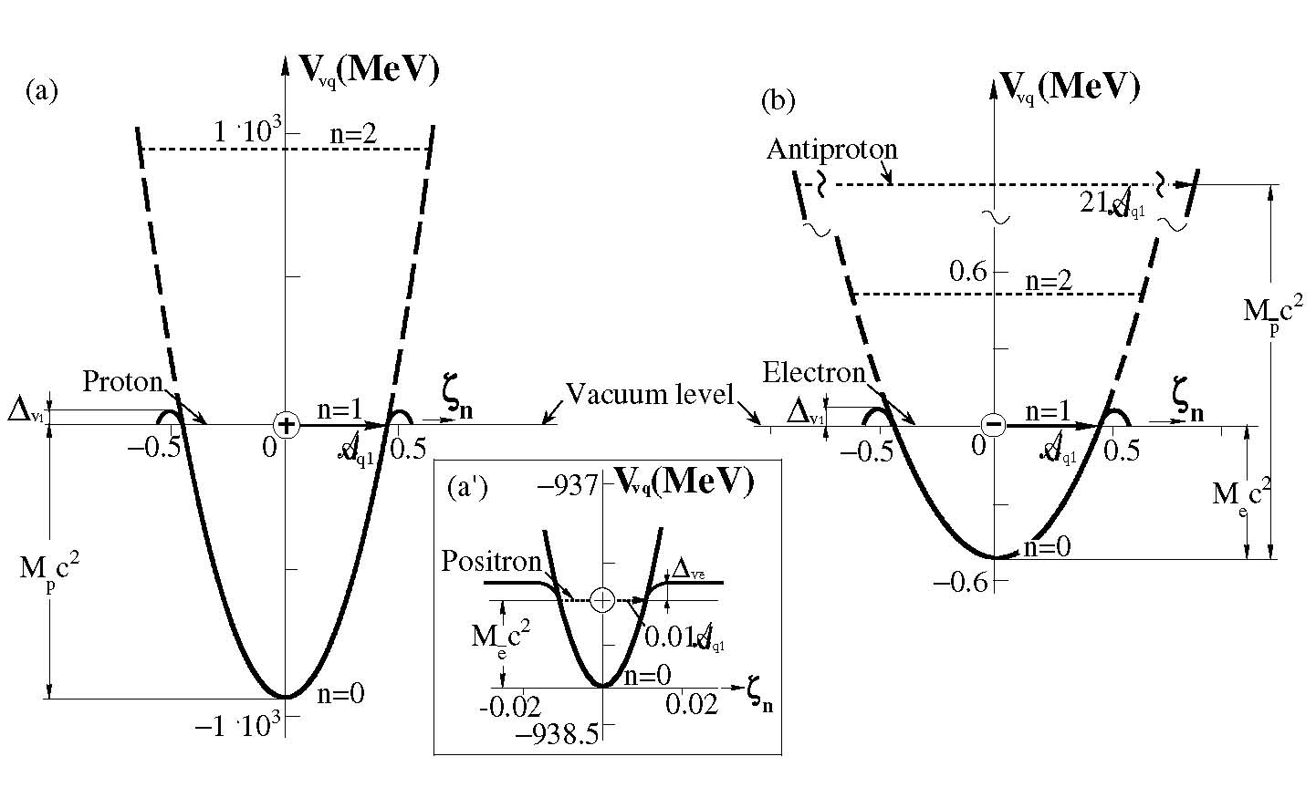
Figure 1: Vacuum potential energy functions $V_{{\mbox{\footnotesize{\rm{v}}}}q}(\zeta_{n})$ versus the centre-of-mass coordinate of a minute extensive charge $q$, $\zeta_{n}$, given by (3) for (a) $q=+e$, and (b) $q=-e$. Used for the plot: $f_{1}=0.9$.

Taking (i)-(iv) together, the creation of particle $p$ or $e$ corresponds to the excitation from energy level $n=0$ (the ground state) to $n=1$ (the first excited state) of the charge $q$ $=+e$ or $-e$ in its potential well $V_{{\mbox{\footnotesize{\rm{v}}}}{\mbox{\scriptsize{$+$}}}en}$ or $V_{{\mbox{\footnotesize{\rm{v}}}}{\mbox{-}}en}$, upon a minimum external energy supply ${\varepsilon}_{exc.m}(=\hbar\omega{}_{\gamma}{})={\varepsilon}_{q1}=M_{p}c^{2}$ or $M_{e}c^{2}$. ${\varepsilon}_{exc.m}$ is thus used for overcoming the potential energy difference $V_{{\mbox{\footnotesize{\rm{v}}}}q0}-V_{{\mbox{\footnotesize{\rm{v}}}}q1}=V_{{\mbox{\footnotesize{\rm{v}}}}q0}-0$, whence

$$\halign{\hbox to\displaywidth{$\hfil\displaystyle#\hfil$}\cr 0.0pt{\hfil$\displaystyle\hfill V_{{\mbox{\footnotesize{\rm{v}}}}q0}=-{\varepsilon}_{exc.m}=-Mc^{2}\qquad(q,M=+e,M_{p};-e,M_{e})\hfill(\ref{eq-Vvqo})\crcr}}$$

And the energy ${\varepsilon}_{q1}$ gained by the charge $+e$ or $-e$ corresponds to the total energy associated with the rest mass $M_{p}$ or $M_{e}$ of the resulting IED particle $p$ or $e$.

Placing (3a),(3) in (2), we obtain the parameterised quantised vacuum potential energy functions of the charges $+e$ and $-e$ respectively versus $\zeta_{n}(=\sqrt{n}\zeta)$ across the interstice about $\zeta_{n}=0$,

$$\halign{\hbox to\displaywidth{$\hfil\displaystyle#\hfil$}\cr 0.0pt{\hfil$\displaystyle\hfill V_{{\mbox{\footnotesize{\rm{v}}}}qn}(\zeta_{n})=Mc^{2}(-1+\frac{4}{f_{1}^{2}}\zeta_{n}^{2})\qquad(q,M=+e,M_{p};-e,M_{e};\ |\zeta|<\mbox{$\frac{1}{2}$}).\hfill(\ref{eq-Vvqnpe})\crcr}}$$

The function $V_{{\mbox{\footnotesize{\rm{v}}}}qn}$ is completely specified by (3) except that $f_{1}$ depends on $\delta_{1}$ through (3b) and is yet to be determined. $f_{1}$ affects the steepness of the $V_{{\mbox{\footnotesize{\rm{v}}}}qn}$ well only; the energy levels of stable particle species (or particle states) therefore are completely specified by (3).

Equations (3), see also the graphical plots in Figure 1a,b, show a strong asymmetry of $V_{{\mbox{\footnotesize{\rm{v}}}}qn}(\zeta_{n})$ with respect to an external charge $+e$ and $-e$: $V_{{\mbox{\footnotesize{\rm{v}}}}{\mbox{\scriptsize{$+$}}}en}(\zeta_{n})$ has a strongly negative depth $-M_{p}c^{2}=-938.27$ MeV (Figure 1a), and $V_{{\mbox{\footnotesize{\rm{v}}}}{\mbox{-}}en}$ has a shallow ”negative” depth $-M_{e}c^{2}=-0.511$ MeV (Figure 1b). This very asymmetry will be directly demonstrated in A.1 through a formal evaluation of the electromagnetic interaction for an external $q$ charge and vacuuon: an external positive charge $+q$ will be strongly attracted by the vacuum, while a negative charge $-q$ be strongly repelled therein. And this is a direct consequence of the asymmetric structure of the vacuuon, of which $-e$ envelops $+e$ (see Sec.4), combined with a ”strong force” effect which onsets at short interaction distances compared to the extension of the vacuuon.

As already entered as an input for the $V_{{\mbox{\footnotesize{\rm{v}}}}qn}$ parameterisation, the proton lies at the first excited stationary state, i.e. energy level $n=1$, of charge $+e$ in the $V_{{\mbox{\footnotesize{\rm{v}}}}{\mbox{\scriptsize{$+$}}}en}$ well, and the electron at level $n=1$ of $-e$ in the $V_{{\mbox{\footnotesize{\rm{v}}}}{\mbox{-}}en}$ well, shown by the solid horizontal lines in Figure 1a and b. The very large mass ratio of $p$ over $e$, $M_{p}/M_{e}\approx 1836$, in retrospect, is a direct reflection of the asymmetry of the two vacuum potentials.

Based on the solutions (2), there is no stationary state below the level $n=1$ for either charge. However, in a pair production out of a vacuuon (Sec. 4) in the vacuum, both its bound vaculeon charges $+e$ and $-e$ (assuming having been firstly disintegrated and now serving as two un-bound external charges) are by a resonance condition (see the end of Sec. 4) simultaneously excited with equal energies, provided a total energy $2\times{\varepsilon}_{exc}=2\times\hbar\omega{}_{\gamma{}}$ is externally supplied. If ${\varepsilon}_{exc}$ is such that $-e$ is excited to its $n=1$ level in the $V_{{\mbox{\footnotesize{\rm{v}}}}{\mbox{-}}en}$ well (Figure 1b), whence $\omega{}_{\gamma{}}=M_{e}c^{2}/\hbar$ and the creation of a stable electron $e$, then $+e$ is excited by the same quantum $\hbar\omega{}_{\gamma{}}$ in the $V_{{\mbox{\footnotesize{\rm{v}}}}{\mbox{\scriptsize{$+$}}}en}$ well (Figure 1a^′), whence the creation of a positron ${\bar{e}}$. The $+e$ of ${\bar{e}}$ is at the level $V_{{\mbox{\footnotesize{\rm{v}}}}{\mbox{\scriptsize{$+$}}}e{\bar{e}}}=V_{{\mbox{\footnotesize{\rm{v}}}}{\mbox{\scriptsize{$+$}}}en}(\mathscr{A}_{{\mbox{\scriptsize{$+$}}}e{\bar{e}}})$ (dotted horizontal line in Figure 1a^′) and has an oscillation amplitude $\mathscr{A}_{{\mbox{\scriptsize{$+$}}}e{\bar{e}}}$. This ${\bar{e}}$ state is far below the $n=1$ (proton) level in the $V_{{\mbox{\footnotesize{\rm{v}}}}{\mbox{\scriptsize{$+$}}}en}$ well, and is not a stationary state. But it would be virtually stable if, as is highly probable, the $e$ simultaneously created has moved away and also no other electron presents nearby for annihilation. This ${\bar{e}}$ will be ”hidden” in the vacuum and not ”free” in the sense said in (IV) earlier.

On the other hand, this excited $+e$ of ${\bar{e}}$ is free to travel from site to site at its own constant potential energy level $V_{{\mbox{\footnotesize{\rm{v}}}}{\mbox{\scriptsize{$+$}}}e{\bar{e}}}$, provided it has a sufficient kinetic energy to ”hop” over a barrier (cf Figure 1a^′), $\Delta_{{\mbox{\footnotesize{\rm{v}}}}_{\bar{e}}}=V_{{\mbox{\footnotesize{\rm{v}}}}{\mbox{\scriptsize{$+$}}}e{\bar{e}}}^{\prime}(z)-V_{{\mbox{\footnotesize{\rm{v}}}}{\mbox{\scriptsize{$+$}}}e{\bar{e}}}(\mathscr{A}_{q{\bar{e}}})$, crossing each two sites. The $\mathscr{A}_{{\mbox{\scriptsize{$+$}}}e{\bar{e}}}$ of $+e$ may be evaluated based on the energy equation for ${\bar{e}}$, $\frac{1}{2}\beta_{{\mbox{\scriptsize{$+$}}}e}\mathscr{A}_{{\mbox{\scriptsize{$+$}}}e{\bar{e}}}^{2}=M_{e}c^{2}$, given by using $\beta_{q}=\beta_{{\mbox{\scriptsize{$+$}}}e}$ for $+e$ in (3) but with the ${\varepsilon}_{exc}$ equal to that of its opposite charge at level $n=1$ (i.e. $M_{e}c^{2}$) for ${\varepsilon}_{q1}$, to be

$$\halign{\hbox to\displaywidth{$\hfil\displaystyle#\hfil$}\cr 0.0pt{\hfil$\displaystyle\hfill\mathscr{A}_{{\mbox{\scriptsize{$+$}}}e{\bar{e}}}=\sqrt{2M_{e}c^{2}/\beta_{{\mbox{\scriptsize{$+$}}}e}}=\sqrt{(M_{e}/M_{p})}\ \mathscr{A}_{{\mbox{\scriptsize{$+$}}}e1}=0.0116\mathscr{A}_{{\mbox{\scriptsize{$+$}}}e1},\hfill(\ref{eq-Acal2})\crcr}}$$

which is exceedingly small. The width of the barrier $\Delta_{{\mbox{\footnotesize{\rm{v}}}}_{\bar{e}}}$, $\delta_{\bar{e}}=b_{\mbox{\footnotesize{\rm{v}}}}-2\times 0.01\mathscr{A}_{q1}\sim b_{\mbox{\footnotesize{\rm{v}}}}$ (assuming $\delta_{1}<<\frac{b_{\mbox{\footnotesize{\rm{v}}}}}{2}$), is thus wide. So after excited to above the barrier $\Delta_{{\mbox{\footnotesize{\rm{v}}}}_{\bar{e}}}$, the charge will be translating across the large distance $\delta_{\bar{e}}\sim b_{\mbox{\footnotesize{\rm{v}}}}$ before entering next $V_{{\mbox{\footnotesize{\rm{v}}}}{\mbox{\scriptsize{$+$}}}en}$ well. From the experimental decay processes of the subatomic particles (e.g. [1]), we observe that, if disregarding the mediators $W^{\pm}$, ${\bar{e}}$ is in fact the only non-composite particle formed of $+e$ which is below the $n=1$ level in the $V_{{\mbox{\footnotesize{\rm{v}}}}{\mbox{\scriptsize{$+$}}}en}$ well. All of the other mass-deficit subatomic particles like $\pi^{+},K^{+},\rho$, manifestly having one-unit charges $+e$’s, are apparently composite particles built ultimately of a lepton $\mu$ and its neutrino, with $\mu$ being built of charge $-e$ in the $V_{{\mbox{\footnotesize{\rm{v}}}}{\mbox{-}}en}$ well.

If on the other hand ${\varepsilon}_{exc}$ is such that $+e$ is excited to the $n=1$ level in the $V_{{\mbox{\footnotesize{\rm{v}}}}{\mbox{\scriptsize{$+$}}}en}$ well (Figure 1a), whence $\omega{}_{\gamma{}}=M_{p}c^{2}/\hbar$ and the creation of a stable proton $p$, then similarly by a resonance condition $-e$ is simultaneously excited by the same energy in the $V_{{\mbox{\footnotesize{\rm{v}}}}{\mbox{-}}en}$ well (Figure 1b), whence the creation of an antiproton ${\bar{p}}$. The charge $-e$ of ${\bar{p}}$ is at the potential energy level $V_{{\mbox{\footnotesize{\rm{v}}}}{\mbox{-}}e{\bar{p}}}=V_{{\mbox{\footnotesize{\rm{v}}}}{\mbox{-}}en}(\mathscr{A}_{{\mbox{-}}\rme{\bar{p}}})$ (dotted horizontal line in Figure 1b) and has an oscillation amplitude $\mathscr{A}_{{\mbox{-}}\rme{\bar{p}}}$. Similarly from $\frac{1}{2}\beta_{{\mbox{-}}e}\mathscr{A}_{{\mbox{-}}e{\bar{p}}}^{2}=M_{p}c^{2}$ given by using $\beta_{q}=\beta_{{\mbox{-}}e}$ in (2) and ${\varepsilon}_{exc}=M_{p}c^{2}$, we formally obtain

$$\halign{\hbox to\displaywidth{$\hfil\displaystyle#\hfil$}\cr 0.0pt{\hfil$\displaystyle\hfill\quad\mathscr{A}_{{\mbox{-}}e{\bar{p}}}=\sqrt{2M_{p}c^{2}/\beta_{{\mbox{-}}e}}=\sqrt{(M_{p}/M_{e})}\ \mathscr{A}_{{\mbox{-}}e1}=21.42\mathscr{A}_{{\mbox{-}}e1},\hfill(\ref{eq-Acal2b})\crcr}}$$

which is many times larger than $\mathscr{A}_{{\mbox{-}}e1}$ of the $-e$ of an electron, as is an inevitable result for $V_{{\mbox{\footnotesize{\rm{v}}}}{\mbox{-}}e{\bar{p}}}>>$ $V_{{\mbox{\footnotesize{\rm{v}}}}{\mbox{-}}e1}$.

Since however the vacuum potential has a mean translation periodicity $b_{\mbox{\footnotesize{\rm{v}}}}$ along any diffusion path and thus is only quadratically well defined up to the vacuum level plus a $\Delta_{{\mbox{\footnotesize{\rm{v}}}}_{1}}$ about $z=\frac{b_{\mbox{\footnotesize{\rm{v}}}}}{2}$, the charge $-e$ of ${\bar{p}}$ of the exceedingly large $\mathscr{A}_{{\mbox{-}}e{\bar{p}}}$ factually traverses many potential wells in each quart of its oscillation period. This motion is no longer properly harmonic; and higher stationary levels than 1, i.e. $n=2,3,\dots$, become unphysical except during charge–vacuuon head-on collisions. The charge $-e$ of ${\bar{p}}$ accordingly will be so energetic as to translate swiftly across many sites in short time, meeting and scattering with other particles and losing its energy easily, until settling down at the next and actually the only lower stationary level in the $V_{{\mbox{\footnotesize{\rm{v}}}}{\mbox{-}}en}$ well, which is the $n=1$ or electron state. That is, the resulting antiproton is short-lived and briefly will descend into a stable electron. This could explain the prominent ”missing” of the antiprotons ${\bar{p}}$’s if all the protons present in nature indeed are produced in $p$—${\bar{p}}$ pair productions.

The above scheme can similarly account for the short lifetimes of the other observational heavier-mass, non-composite subatomic particles made of one-unit charges, actually the leptons $\mu,\tau$ only which are built of one-unit $-e$ in the $V_{{\mbox{\footnotesize{\rm{v}}}}{\mbox{-}}en}$ well, if disregarding the mediators, similarly based on the experimental decay processes of subatomic particles. All the other heavier-mass baryons such as ${\mit\Omega}^{\mbox{-}}$, ${\mit\Lambda}$’s, $\Sigma$’s and mesons such as $\pi^{\mbox{-}},D^{\pm}$, etc. having either one-unit $-e$ or (as earlier remarked)$+e$, are apparently composite particles ultimately built of $\mu$’s and their neutrinos.

4 Vacuuonic potentials. Pair productions

A vacuuon (e.g. ${\rm v}_{1}$ in Figure 4a) by construction[2, 9] consists of a positive charge $+e$ seated on a minute sphere of radius $r_{p_{{\mbox{\tiny{v}}}}}$ at the centre, and a negative charge $-e$ on a concentric spherical shell of thickness $2r_{o}$ and radius $r_{n_{{\mbox{\tiny{v}}}}}$ about ${p_{{\mbox{\tiny{v}}}}}$, termed as a p-vaculeon ($p_{\mbox{\footnotesize{\rm{v}}}}$) and n-vaculeon ($n_{\mbox{\footnotesize{\rm{v}}}}$). The ${p_{{\mbox{\tiny{v}}}}},{n_{{\mbox{\tiny{v}}}}}$ have spins $\frac{\hbar}{2}$ each; in their bound state in a vacuuon their spin magnetic moments are oriented in opposite directions in each others’ magnetic fields. The vacuuon structure, as a building entity of the substantial vacuum, is constructed based on overall experimental indications, most directly the pair production and annihilation experiments in particular[2, 9, 13]; see further the discussion after (4) later.

The $r_{p_{{\mbox{\tiny{v}}}}},r_{n_{{\mbox{\tiny{v}}}}}$ represent the most probable radii of the practically extensive ${p_{{\mbox{\tiny{v}}}}},{n_{{\mbox{\tiny{v}}}}}$ (similarly as the single charge $q$ in Sec. 2) at the scale $b_{\mbox{\footnotesize{\rm{v}}}}$, and $r_{o}$ is said in a similar sense. We presently lack experimental information either on their direct values or for their theoretical evaluation; although definitely they must be (much) smaller than $\frac{b_{\mbox{\footnotesize{\rm{v}}}}}{2}$. For the illustration below we shall take the $r_{p_{{\mbox{\tiny{v}}}}},r_{o}$ values by their average, $\frac{1}{2}(r_{p_{{\mbox{\tiny{v}}}}}+r_{o})=\sigma$. And we set the vacuuon radius $r_{\mbox{\footnotesize{\rm{v}}}}$, $=r_{n_{{\mbox{\tiny{v}}}}}+r_{o}$, as the contact radius of the vacuuons on a simple cubic lattice (Sec. 3), so $r_{\mbox{\footnotesize{\rm{v}}}}=\frac{b_{\mbox{\footnotesize{\rm{v}}}}}{2}$, see Figure 4a. The focus of our discussion below will be to demonstrate the characteristics of the interactions rather than to perform an accurate numerical calculation.

Figure 4 (left graphs). Vacuuons ${\rm v}_{i}$, with ${\rm v}_{1}$ at $z=0$, arranged on a simple cubic lattice (a) in zero external field, and (b)–(c) in the field of an external charge $+q$ in the interstice $B$; $+q$ is moving toward ${\rm v}_{1}$ at a finite velocity. In (c), $+q$ has collided with ${n_{{\mbox{\tiny{v}}}}}$ and in turn knocked ${n_{{\mbox{\tiny{v}}}}}$ into colliding with ${p_{{\mbox{\tiny{v}}}}}$ to their closed approaches each; at the same time, a $2\gamma{}$ wave of energy $2\hbar\omega{}_{\gamma}{}(\geq 2Mc^{2})$ is incident on to ${\rm v}_{1}$.

Figure 4 (right graphs). (a) Solid curve: ${p_{{\mbox{\tiny{v}}}}}$—${n_{{\mbox{\tiny{v}}}}}$ interaction potential energy $V_{{p_{{\mbox{\tiny{v}}}}}{n_{{\mbox{\tiny{v}}}}}}(\zeta)$ given by (4) for vacuuon ${\rm v}_{1}$ in zero external field (as in Figure 4a), $\zeta=r/b_{\mbox{\footnotesize{\rm{v}}}}$. Dashed curve 2 and dotted curve 3 ($\zeta>r_{\mbox{\footnotesize{\rm{v}}}}$): potential energies of ${p_{{\mbox{\tiny{v}}}}}$ and ${n_{{\mbox{\tiny{v}}}}}$ of ${\rm v}_{1}$, $V_{{p_{{\mbox{\tiny{v}}}}}{n_{{\mbox{\tiny{v}}}}}{\mbox{\scriptsize{$+$}}}q}(\zeta)$ and $V_{{n_{{\mbox{\tiny{v}}}}}{p_{{\mbox{\tiny{v}}}}}{\mbox{\scriptsize{$+$}}}q}(\zeta)$ given by (A)–(A) in the field of external charge $+q$ as in Figure 4b. The rapid rising part of curve 2 and curve 3^′: the two potential energy functions $V_{{p_{{\mbox{\tiny{v}}}}}{n_{{\mbox{\tiny{v}}}}}{\mbox{\scriptsize{$+$}}}q}(\zeta)$ and $V_{{n_{{\mbox{\tiny{v}}}}}{p_{{\mbox{\tiny{v}}}}}{\mbox{\scriptsize{$+$}}}q}(\zeta)$ when $+q$, ${n_{{\mbox{\tiny{v}}}}}$ and ${p_{{\mbox{\tiny{v}}}}}$ are as positioned in Figure 4c. Corresponding curves $2$, $3^{\prime}$ for $-q$ are shown in (a^′). Short-dot-dashed curves: the function $V_{{\mbox{\footnotesize{\rm{v}}}}{\mbox{\scriptsize{$+$}}}en}$ in (a) and $V_{{\mbox{\footnotesize{\rm{v}}}}{\mbox{-}}en}$ in (a^′) given by (3). Used for the plots: $\sigma=0.1b_{\mbox{\footnotesize{\rm{v}}}}$ (thus $u_{1}=14400$ MeV), ${\mbox{\scriptsize{$N$}}}=12$, $d=0.01b_{\mbox{\footnotesize{\rm{v}}}}$. At $r_{m}=(g{\mbox{\scriptsize{$N$}}})^{\frac{1}{{\mbox{\tiny{$N$}}}-1}}\sigma=0.859\sigma$, $\frac{\partial V_{{p_{{\mbox{\tiny{v}}}}}{n_{{\mbox{\tiny{v}}}}}}}{\partial r}=0$ and $V_{{p_{{\mbox{\tiny{v}}}}}{n_{{\mbox{\tiny{v}}}}}m}(r_{m})=-\frac{u_{1}}{2}(g{\mbox{\scriptsize{$N$}}})^{-\frac{1}{{\mbox{\tiny{$N$}}}-1}}[\frac{{\mbox{\scriptsize{$N$}}}-1}{{\mbox{\scriptsize{$N$}}}}]=-0.534u_{1}.$ (b) Interaction potential energy function $V_{{\mbox{\footnotesize{\rm{v}}}}_{1}{\mbox{\scriptsize{$+$}}}q}$ (solid curve), given by (Ab), between vacuuon ${\rm v}_{1}$ and external charge $+q$ of position $\zeta$ as in Figure 4b; and $V_{{\mbox{\footnotesize{\rm{v}}}}_{1}{\mbox{-}}q}$ (dashed curve) between ${\rm v}_{1}$ and $-q$. Values used for the plots are as in (a).

In zero external field, the two vaculeon charges $+e$ and $-e$ of a vacuuon, say the ${\rm v}_{1}$ at $z=0$ in Figure 4a, interact each other by a Coulomb attraction, $\mathscr{V}_{{p_{{\mbox{\tiny{v}}}}}{n_{{\mbox{\tiny{v}}}}}}^{coul}=-\frac{e^{2}}{4\pi\epsilon_{0}r}=u_{0}\frac{r_{\mbox{\footnotesize{\rm{v}}}}}{r}=u_{1}\frac{\sigma}{r}$, and a short range repulsion, $\mathscr{V}_{{p_{{\mbox{\tiny{v}}}}}{n_{{\mbox{\tiny{v}}}}}}^{rep}=gu_{1}(\frac{\sigma}{r})^{\mbox{\tiny{$N$}}}$, where $u_{o}=\frac{e^{2}}{4\pi\epsilon_{0}(b_{\mbox{\footnotesize{\rm{v}}}}/2)}=2879.9$ MeV for $r_{\mbox{\footnotesize{\rm{v}}}}=\frac{b_{\mbox{\footnotesize{\rm{v}}}}}{2}=0.5\times 10^{-18}$ m, $u_{1}=u_{o}(r_{\mbox{\footnotesize{\rm{v}}}}/\sigma)$, and $g=\frac{\pi\sigma^{2}}{4\pi r_{n_{{\mbox{\tiny{v}}}}}^{2}}=\frac{\sigma^{2}}{4r_{n_{{\mbox{\tiny{v}}}}}^{2}}$ is the fraction of charge of the segment, of size $\pi\sigma^{2}$ on the extensive ${n_{{\mbox{\tiny{v}}}}}$ shell of an area $4\pi r_{n_{{\mbox{\tiny{v}}}}}^{2}$, which makes direct contact with ${p_{{\mbox{\tiny{v}}}}}$. The ${\mbox{\scriptsize{$N$}}},\sigma$ values are to be determined. The total ${p_{{\mbox{\tiny{v}}}}}$, ${n_{{\mbox{\tiny{v}}}}}$ interaction potential energy per vaculeon is thus

$$\halign{\hbox to\displaywidth{$\hfil\displaystyle#\hfil$}\cr 0.0pt{\hfil$\displaystyle\hfill V_{{p_{{\mbox{\tiny{v}}}}}{n_{{\mbox{\tiny{v}}}}}}(r)=\frac{1}{2}(\mathscr{V}_{{p_{{\mbox{\tiny{v}}}}}{n_{{\mbox{\tiny{v}}}}}}^{rep}(r)+\mathscr{V}_{{p_{{\mbox{\tiny{v}}}}}{n_{{\mbox{\tiny{v}}}}}}^{coul}(r))=\frac{u_{1}}{2}\left[g\left(\frac{\sigma}{r}\right)^{{\mbox{\tiny{$N$}}}}-\frac{\sigma}{r}\right]\hfill(\ref{eqVpn})\crcr}}$$

See also the graphical plot of $V_{{p_{{\mbox{\tiny{v}}}}}{n_{{\mbox{\tiny{v}}}}}}(r)$ in Figure 4a (solid curve 1), where ${\mbox{\scriptsize{$N$}}}=12$ (Lennard-Jones’ value) and $\sigma=0.1b_{\mbox{\footnotesize{\rm{v}}}}$ are used for the illustration.

At $r>>r_{p_{{\mbox{\tiny{v}}}}}$, ${n_{{\mbox{\tiny{v}}}}}$ is acted on by ${p_{{\mbox{\tiny{v}}}}}$ by (mainly) an attractive force $F_{{p_{{\mbox{\tiny{v}}}}}{n_{{\mbox{\tiny{v}}}}}}=-\frac{\partial\mathscr{V}_{{p_{{\mbox{\tiny{v}}}}}{n_{{\mbox{\tiny{v}}}}}}}{\partial r}$ $\approx-\frac{\partial\mathscr{V}_{{p_{{\mbox{\tiny{v}}}}}{n_{{\mbox{\tiny{v}}}}}}^{coul}}{\partial r}$, where $\mathscr{V}_{{p_{{\mbox{\tiny{v}}}}}{n_{{\mbox{\tiny{v}}}}}}=2V_{{p_{{\mbox{\tiny{v}}}}}{n_{{\mbox{\tiny{v}}}}}}$. This, in the zero mass representation, is counterbalanced by a magnetic force $F_{m}$ on the spinning $n$-vaculeon charge on the spherical envelope in the magnetic field produced by spinning motion of $p$-vaculeon charge (Appendix A of [2]), $F_{m},=-F_{p_{\mbox{\tiny{v}}}n_{\mbox{\tiny{v}}}}$. The equality defines the equilibrium radius $r_{n_{{\mbox{\tiny{v}}}}}(=\frac{b_{\mbox{\footnotesize{\rm{v}}}}}{2}-\sigma)$, at which $\mathscr{V}_{{p_{{\mbox{\tiny{v}}}}}{n_{{\mbox{\tiny{v}}}}}}(r_{n_{{\mbox{\tiny{v}}}}})\dot{=}-u_{1}(\sigma/r_{n_{{\mbox{\tiny{v}}}}})=-3599.9$ MeV, or $V_{{p_{{\mbox{\tiny{v}}}}}{n_{{\mbox{\tiny{v}}}}}}(r_{n_{{\mbox{\tiny{v}}}}})=-1799.9$ MeV; accordingly, ${n_{{\mbox{\tiny{v}}}}}$ has a spin kinetic energy ${\cal E}_{{n_{{\mbox{\tiny{v}}}}}k}=-\frac{1}{2}\mathscr{V}_{{p_{{\mbox{\tiny{v}}}}}{n_{{\mbox{\tiny{v}}}}}}$ and Hamiltonian ${\cal E}_{{n_{{\mbox{\tiny{v}}}}}t}=\mathscr{V}_{{p_{{\mbox{\tiny{v}}}}}{n_{{\mbox{\tiny{v}}}}}}+{\cal E}_{{n_{{\mbox{\tiny{v}}}}}k}=\frac{1}{2}\mathscr{V}_{{p_{{\mbox{\tiny{v}}}}}{n_{{\mbox{\tiny{v}}}}}}$. This $\mathscr{V}_{{p_{{\mbox{\tiny{v}}}}}{n_{{\mbox{\tiny{v}}}}}}$, of a GeV scale, is far too deep for the vaculeon pair to be disintegrated to the vacuum level, by merely a supply of an excitation energy $2{\varepsilon}_{exc.m}$ given by (3), or

$$\halign{\hbox to\displaywidth{$\hfil\displaystyle#\hfil$}\cr 0.0pt{\hfil$\displaystyle\hfill 2\times{\varepsilon}_{exc}=2\times\hbar\omega{}_{\gamma{}}\geq 2\times Mc^{2}=\frac{1}{2}\beta_{q}(\sqrt{2}\mathscr{A}_{q1})^{2}\qquad(M=M_{p},M_{e};\ q=+e,-e)\hfill(\ref{eq-exceng})\crcr}}$$

which are $2\times 938.27$, $2\times$ 0.511 MeV for the $p$—${\bar{p}}$, $e$—${\bar{e}}$ pair productions. This $2{\varepsilon}_{exc}$ is merely enough to impart masses to a pair of dissociated vaculeon charges.

Inevitably, before the condition (4) becomes legible, an additional energy, as enormous as $2\times(V_{{\mbox{\footnotesize{\rm{v}}}}q0}-V_{{p_{{\mbox{\tiny{v}}}}}{n_{{\mbox{\tiny{v}}}}}}(r_{n_{{\mbox{\tiny{v}}}}}))\sim 3600$ MeV for $e$—${\bar{e}}$ production or $1720$ MeV for $p$—${\bar{p}}$ production, needs firstly be supplied so as to disassociate the pair of bound vaculeons of the ${\rm v}_{1}$ here to at or above the ground state of the charge, $V_{{\mbox{\footnotesize{\rm{v}}}}q0}$. Such an enormous energy may be practically supplied if the two vaculeons are simultaneously approached by a charged particle (e.g. a nucleon) $q$ at very short distance and thereby repelled to above $V_{{\mbox{\footnotesize{\rm{v}}}}q0}$; an external $q$ thus needs be in the proximity (like the $+q$ in the interstice $B$ in Figure 4b) and moving at an adequate speed toward ${\rm v}_{1}$. A possible such process is illustrated in Figure 4c. The corresponding potential energies of ${p_{{\mbox{\tiny{v}}}}}$,${n_{{\mbox{\tiny{v}}}}}$ in the presence of $+q$, of coordinate $z$, and similarly of $-q$, $V_{{p_{{\mbox{\tiny{v}}}}}{n_{{\mbox{\tiny{v}}}}}\pm q}(z)$,$V_{{n_{{\mbox{\tiny{v}}}}}{p_{{\mbox{\tiny{v}}}}}\pm q}(z)$ as functions of the position $z$ of $+q$ or $-q$ are given by (A)–(A), A.2. As the graphical plots, the dashed curves 2 and dotted curves 3 to $3^{\prime}$ in Figure 4 a,a^′ directly show, the two potential energy functions rise each rapidly to above $V_{{\mbox{\footnotesize{\rm{v}}}}q0}$ at the closest approach between $+q,{n_{{\mbox{\tiny{v}}}}}$ and ${p_{{\mbox{\tiny{v}}}}}$ (Figure 4c), i.e. at $z\sim 3\sigma$. The vaculeons ${p_{{\mbox{\tiny{v}}}}}$ and ${n_{{\mbox{\tiny{v}}}}}$ are now effectively no longer bound each other, being as if separated infinitely apart.

If these, as soon as after their dissociation, are impinged by a $\gamma{}$ wave (see Figure 4c) of an energy $2{\varepsilon}_{exc}=2\hbar\omega{}_{\gamma}{}$ fulfilling (4), e.g. $\omega{}_{\gamma}{}=m_{p}c^{2}/\hbar$, then upon absorption of $2{\varepsilon}_{exc}$ by a ”resonance condition” (see below) the vaculeon charges $+e,-e$ will have been each endowed with an oscillation energy $\hbar\omega{}_{p}=m_{p}c^{2}$. $+e$ is now promoted to the energy level $n=1$ in the $V_{{\mbox{\footnotesize{\rm{v}}}}{\mbox{\scriptsize{$+$}}}en}$ well at one site (short-dot-dashed curve in Figure 4a); and $-e$ to the level of ${\bar{p}}$ in the $V_{{\mbox{\footnotesize{\rm{v}}}}{\mbox{-}}en}$ well, by a probable tendency, in another site located in the opposite direction to the displacement of $+e$, since the charges $+e,-e$ producing (or absorbing) the same radiation ${\bf{E}}$ field have opposite oscillation displacements. And similarly for $\omega{}_{\gamma}{}=m_{e}c^{2}/\hbar$, with the charge $-e$ promoted to level $n=1$ in the $V_{{\mbox{\footnotesize{\rm{v}}}}{\mbox{-}}en}$ well (short-dot-dashed curve in Figure 4a^′), and $+e$ to the level of ${\bar{e}}$ in the $V_{{\mbox{\footnotesize{\rm{v}}}}{\mbox{\scriptsize{$+$}}}en}$ well. These are the $p$—${\bar{p}}$ and $e$—${\bar{e}}$ pair productions of the reaction equations

$$\halign{\hbox to\displaywidth{$\hfil\displaystyle#\hfil$}\cr 0.0pt{\hfil$\displaystyle\hfill 2\gamma{}\rightarrow p+{\bar{p}},\quad\quad 2\gamma{}\rightarrow e+{\bar{e}}.\hfill(\ref{eq-pair1})\crcr}}$$

The pair of particles produced will be at rest if ${\mit\Omega}=Mc^{2}/\hbar$ or will have a residual velocity $\upsilon=c\sqrt{1-1/\gamma{}^{2}}$ if $\omega{}=\gamma{}{\mit\Omega}>{\mit\Omega}$, i.e. $\gamma{}>1$.

The reaction equations (4), together with the preceding energy criterion (4) and the requirement for the presence of a nucleus (or nuclei) in a pair production, are in complete agreement with experiment. Entirely as an experimental reaction equation, (4) are expressed such that they each inform explicitly all of ”observables” before and after a pair production. In particular, (4) inform that both charges ($+e,-e$) and spins ($\frac{\hbar}{2},\frac{\hbar}{2}$) are present on their right-hand sides, but not the left-hand sides. And the external energy supply $2{\varepsilon}_{exc}=2Mc^{2}$ is only to ascribe dynamical masses to the pair of vaculeon charges $+e,-e$ (which have zero rest masses), or equivalently, (dynamical) rest masses to the resulting IED particles in each reaction process, $e,{\bar{e}}$ or $p,{\bar{p}}$. So the charges $+e,-e$ which carry a potential energy $V_{{p_{{\mbox{\tiny{v}}}}}{n_{{\mbox{\tiny{v}}}}}}(r_{n_{{\mbox{\tiny{v}}}}})$ at the particles’ production as given by (4), and their spins $\frac{\hbar}{2}$’s which carry a kinetic energy, must exist in the vacuum, whence the vaculeons composing a vacuuon, so as to satisfy the requirement of energy conservation. Similar discussion was made in terms of the pair annihilation in [2, 9, 13].

Supplemental remarks regarding the pair production: (i) The resonance condition. In mechanical terms, as follows from Sec. 2, the dielectric vacuum is induced with an elasticity in the presence of an external charge ($q$) nearby. And the electromagnetic ($\gamma{}$) wave, of a wavelength $\lambda_{\gamma}{}\sim 1.3\times 10^{-15}$ or $\sim 2.4\times 10^{-12}$ m, is an elastic wave propagated in the vacuum by means of the elastic deformations of the vacuum, or in other terms, of the oscillations of coupled oscillators each composed of (tremendously) many vacuuons (of size $\sim 10^{-18}$ m each). So relative to the extensive $\gamma{}$ wave, the pair of vaculeons ${p_{{\mbox{\tiny{v}}}}},{n_{{\mbox{\tiny{v}}}}}$ in a vacuuon (the ${\rm v}_{1}$ above) are just a minute point on a large oscillator. They will respond to the $\gamma{}$ wave as one point, practically the only point in the large oscillator being in the (internal) mode of resonance absorption to the quanta $2\hbar\omega{}_{r}$ of the $\gamma{}$ wave, assuming no other bound vaculeons in the large oscillator are dissociated to above level $V_{{\mbox{\footnotesize{\rm{v}}}}q0}$.

(ii) The incident $\gamma{}$ wave of energy $2{\varepsilon}_{exc}$ is an extensive electromagnetic wave train (as schematically shown in Figure 4c) of length $L_{\varphi}$ and effective amplitude $A_{q2}=\frac{\sqrt{2}}{\sqrt{t_{\varphi 2.0}/(1/\omega{})}}\mathscr{A}_{q1}$[16]. Accordingly, the ”absorption of $2{\varepsilon}_{exc}$” is a gradual, continuous process spanning a total duration $t_{\varphi 1.0}$, in which the wave train front runs at the velocity of light $c$ on to the two vaculeon charges $+e$ and $-e$ of ${\rm v}_{1}$, and be thereby absorbed by them (by a certain fraction) continuously. Two new waves of the same $\omega{}$, and of amplitude $A_{q1}$ each, are subsequently continuously re-emitted by the two charges, and then, together with the transmitted fraction, re-absorbed after reflecting back from surrounding walls.

(iii) At the end of one $t_{\varphi 1.0}$, two full wave trains (i.e. for the fraction $a_{1}+a_{2}=1$) maintain the same $L_{\varphi}$, and same total $2{\varepsilon}=2mc^{2}$, and $2p=2{\varepsilon}/c=2mc$ (i.e. the linear momentum, which is conserved in this sense) as the incident one. These two wave trains have now become the respective (internal) components of the (IED) particle and antiparticle just produced.

Appendix A Electromagnetic interaction

A.1 Interactions at larger distances up to a closest approach

As shown in Figure 4b (Sec. 4), the vacuuon ${\rm v}_{1}$ at $z=0$ is polarised by the external charge $+q$ in the interstice $B$, moving from initial position say $z=\frac{b_{\mbox{\footnotesize{\rm{v}}}}}{\sqrt{2}}$ toward ${\rm v}_{1}$ at a finite speed. We shall express the ${\rm v}_{1}$—$+q$ and ${\rm v}_{1}$—$-q$ interaction potentials in electromagnetic terms below, and shall do so by situating ourselves in the frame where the mass centre of ${\rm v}_{1}$ is not moved during the interaction. (This frame approximately corresponds to the frame fixed to the vacuum if ${\rm v}_{1}$ and its surrounding vacuuons can not move freely due to attachment to a fixed matrix of charged particles, but their configuration may be locally deformed under the dynamical impact of $q$.) In this frame, the ${p_{{\mbox{\tiny{v}}}}}$ and ${n_{{\mbox{\tiny{v}}}}}$ vaculeons of the polarised vacuuon ${\rm v}_{1}$ are displaced from the fixed position $z=0$ to $-\frac{d}{2}$ and $+\frac{d}{2}$. Since $r_{n_{{\mbox{\tiny{v}}}}}>>\sigma$, we shall regard the ${p_{{\mbox{\tiny{v}}}}}$ and $q$ as point like and the ${n_{{\mbox{\tiny{v}}}}}$- spherical shell extensive in respect to their short range interactions.

$+q$ interacts with a charge element $dq_{1}$ on the extensive spherical shell of ${n_{{\mbox{\tiny{v}}}}}$ by a Coulomb attraction $dF=\frac{dq_{1},q}{4\pi\epsilon_{o}\ell}$. Integration over the entire shell gives the total attraction of $+q$ and ${n_{{\mbox{\tiny{v}}}}}$ as [2] $F\dot{=}-\frac{u_{1}\sigma}{r_{n_{{\mbox{\tiny{v}}}}}^{2}}(\frac{r_{n_{{\mbox{\tiny{v}}}}}}{z})^{n+1}$, with $n=15.7$, which is strongly short ranged (whence a ”strong force”). Accordingly $V^{coul}_{{n_{{\mbox{\tiny{v}}}}}{\mbox{\scriptsize{$+$}}}q}=-\frac{1}{2}\int^{\infty}_{z}Fdz\dot{=}-\frac{u_{1}\sigma}{2r_{n_{{\mbox{\tiny{v}}}}}n}(\frac{r_{n_{{\mbox{\tiny{v}}}}}}{z})^{n}$. Because of the simple symmetry of the ${n_{{\mbox{\tiny{v}}}}}$-shell with respect to $+q$, for a better physical transparency we below express this interaction alternatively by representing ${n_{{\mbox{\tiny{v}}}}}$ effectively as two one-half charges $\frac{e}{2},\frac{e}{2}$ projected on the $z$ axis at $-{\bar{r}}_{n_{{\mbox{\tiny{v}}}}},+{\bar{r}}_{n_{{\mbox{\tiny{v}}}}}$, with ${\bar{r}}_{n_{{\mbox{\tiny{v}}}}}=r_{\mbox{\footnotesize{\rm{v}}}}/2$[2], as

$$\halign{\hbox to\displaywidth{$\hfil\displaystyle#\hfil$}\cr 0.0pt{\hfil$\displaystyle\hfill V_{{n_{{\mbox{\tiny{v}}}}}{\mbox{\scriptsize{$+$}}}q}^{coul}=-\frac{u_{1}}{4}\left[\frac{\sigma}{z-({\bar{r}}_{n_{{\mbox{\tiny{v}}}}}+\frac{d}{2})}+\frac{\sigma}{z+({\bar{r}}_{n_{{\mbox{\tiny{v}}}}}-\frac{d}{2})}\right]=-\frac{u_{1}\sigma\eta}{2(z-\frac{d}{2})},\quad\eta=\frac{1}{1-({\bar{r}}_{n_{{\mbox{\tiny{v}}}}}/(z-\frac{d}{2}))^{2}}.\hfill\cr 0.0pt{\hfil$\displaystyle\hfill(\ref{eq-Vpm-qpvnv1})\crcr}}}$$

In addition, $+q$ interacts with ${n_{{\mbox{\tiny{v}}}}}$ similarly through ${n_{{\mbox{\tiny{v}}}}}$ of a fractional charge $gq$ as in (4) by a short range repulsion, $V_{{n_{{\mbox{\tiny{v}}}}}{\mbox{\scriptsize{$+$}}}q}^{rep}=\frac{u_{1}}{2}g\left(\frac{\sigma}{z-(r_{n_{{\mbox{\tiny{v}}}}}+\frac{d}{2})}\right)^{\mbox{\tiny{$N$}}}$. And, with the ${n_{{\mbox{\tiny{v}}}}}$-shell in between, $+q$ interacts with ${p_{{\mbox{\tiny{v}}}}}$ by a Coulomb repulsion only, $V_{{p_{{\mbox{\tiny{v}}}}}{\mbox{\scriptsize{$+$}}}q}^{coul}=\frac{u_{1}}{2}\frac{\sigma}{z+\frac{d}{2}}$ for $z\geq 4\sigma$. Adding the terms above, we obtain the interaction potential energy of $+q$ with vacuuon ${\rm v}_{1}$, and similarly of $-q$ with ${\rm v}_{1}$ after corresponding sign changes, as

$$\halign{\hbox to\displaywidth{$\hfil\displaystyle#\hfil$}\cr 0.0pt{\hfil$\displaystyle\hfill V_{{\mbox{\footnotesize{\rm{v}}}}_{1}\pm q}=V_{{n_{{\mbox{\tiny{v}}}}}\pm q}^{rep}+V_{{n_{{\mbox{\tiny{v}}}}}\pm q}^{coul}+V_{{p_{{\mbox{\tiny{v}}}}}\pm q}^{coul}=\frac{u_{1}}{2}\left[g\left(\frac{\sigma}{z-(r_{n_{{\mbox{\tiny{v}}}}}\pm\frac{d}{2})}\right)^{\mbox{\tiny{$N$}}}\mp\frac{\sigma\eta}{(z\mp\frac{d}{2})}\pm\frac{\sigma}{(z\pm\frac{d}{2})}\right],\hfill\cr 0.0pt{\hfil$\displaystyle\hfill V_{{\mbox{\footnotesize{\rm{v}}}}_{1}\pm q}\dot{=}\frac{u_{1}}{2}\left[g\left(\frac{\sigma}{z-(r_{n_{{\mbox{\tiny{v}}}}}\pm\frac{d}{2})}\right)^{\mbox{\tiny{$N$}}}\mp\frac{\sigma(\eta-1)}{z}-\frac{\sigma d(\eta+1)}{2z^{2}}\right],\quad\eta=\frac{1}{1-({\bar{r}}_{n_{{\mbox{\tiny{v}}}}}/(z\mp\frac{d}{2}))^{2}},\hfill\cr 0.0pt{\hfil$\displaystyle\hfill(\ref{eq-Vpm-qpvnv})\crcr}}}}$$

where (Ab) is given after expanding the second and third terms of (Aa) in $\frac{d}{2z}$ and retaining the respective two first leading terms. The last term in (Ab), $-\frac{u_{1}\sigma d(\eta+1)}{4z^{2}}$, represents the interaction energy of the ${n_{{\mbox{\tiny{v}}}}}$ vaculeon dipole moment, ${\bf p}_{n_{{\mbox{\tiny{v}}}}}=ed\hat{z}$, with the static Coulomb field of charge $q$, ${\bf{E}}_{q}=\frac{u_{1}\sigma(\eta+1)}{2ez^{2}}\hat{z}$, and this may be directly obtained as $V_{dip\pm q}=\frac{1}{2}{\bf p}_{n_{{\mbox{\tiny{v}}}}}\cdot{\bf{E}}_{q}=-\frac{u_{1}\sigma d(\eta+1)}{4z^{2}}$. Since for small $d$ there is always $\eta>$( or $>>)1$, at $z-\frac{3}{2}>{\bar{r}}_{n_{{\mbox{\tiny{v}}}}}$, $V_{dip\pm q}$ is thus an attraction for either $+q$ or $-q$. The second term in $V_{{\mbox{\footnotesize{\rm{v}}}}_{1}\pm q}$ of (Ab), $\pm\frac{\sigma}{(z\pm\frac{d}{2})}=V_{{n_{{\mbox{\tiny{v}}}}}\pm q}^{coul}$ is a main attraction term between ${\rm v}_{1}$ and $+q$, and is a repulsion between ${\rm v}_{1}$ and $-q$. The sum of the interactions of $q$ with all surrounding vacuuons up to an intermediate range, $\sum_{i}V_{{\mbox{\footnotesize{\rm{v}}}}_{i}q}$, gives the $V_{{\mbox{\footnotesize{\rm{v}}}}q}$ of Sec. 2.

As the graphical plots in Figure 4 b directly show, from larger $z$ down to a closest approach at $z=r_{\mbox{\footnotesize{\rm{v}}}}$, the potential $V_{{\mbox{\footnotesize{\rm{v}}}}_{1}{\mbox{\scriptsize{$+$}}}q}$ (solid curve) for the positive charge $+q$ is strongly negative, while $V_{{\mbox{\footnotesize{\rm{v}}}}_{1}{\mbox{-}}q}$ (dotted curve) for $-q$ is positive for a wide range of $d$ value ($d=0.01b_{\mbox{\footnotesize{\rm{v}}}}$ for the plots).

A.2 Dynamical interactions after $q,\mbox{${n_{{\mbox{\tiny{v}}}}}$}$ closest approach

At about $z=r_{\mbox{\footnotesize{\rm{v}}}}$, $+q$ and the segment ${n_{{\mbox{\tiny{v}}}}^{{\rm ef}}}$ of the ${n_{{\mbox{\tiny{v}}}}}$-shell (cf Figure 4c) are at closest approach. And the $+q$—${n_{{\mbox{\tiny{v}}}}}$ interaction potential, $V_{{n_{{\mbox{\tiny{v}}}}}+q}=V_{{n_{{\mbox{\tiny{v}}}}}+q}^{rep}+V_{{n_{{\mbox{\tiny{v}}}}}+q}^{coul}$ as given by the sum of first two terms in (Aa), shown by the dotted curve $3$ in Figure 4a, rises rapidly.

From $z=r_{\mbox{\footnotesize{\rm{v}}}}$ downward, $+q$ continues to move toward ${p_{{\mbox{\tiny{v}}}}}$, now together with ${n_{{\mbox{\tiny{v}}}}}$ while impressing on the segment ${n_{{\mbox{\tiny{v}}}}^{{\rm ef}}}$ (which has the coordinate $z^{\prime}=z-2\sigma$) of ${n_{{\mbox{\tiny{v}}}}}$ a constant repulsion $V_{{n_{{\mbox{\tiny{v}}}}}\mathbin{q\mkern-11.0mu-}}^{rep}(z-z^{\prime})=g(\frac{\sigma}{2\sigma})^{\mbox{\tiny{$N$}}}=g(\frac{1}{2})^{\mbox{\tiny{$N$}}}$ (with the steep sector of the dotted curve 3 sweeping across the region, ending at curve $3^{\prime}$). In addition, $+q$ interacts with $n_{\mbox{\footnotesize{\rm{v}}}}$ by a Coulomb potential $V_{{n_{{\mbox{\tiny{v}}}}}{\mbox{\scriptsize{$+$}}}q}^{coul}(z)|_{z=r_{n_{{\mbox{\tiny{v}}}}}}=-\frac{u_{1}\sigma\eta}{2(r_{n_{{\mbox{\tiny{v}}}}}-d/2)}$ as given after (A); and with ${p_{{\mbox{\tiny{v}}}}}$ by the $V^{coul}_{{p_{{\mbox{\tiny{v}}}}}{\mbox{\scriptsize{$+$}}}q}=\frac{u_{1}\sigma}{2(z+d/2)}$ as before. ${p_{{\mbox{\tiny{v}}}}}$ interacts with ${n_{{\mbox{\tiny{v}}}}}$, as a very crude approximation here, by the constant Coulomb potential $V_{{p_{{\mbox{\tiny{v}}}}}{n_{{\mbox{\tiny{v}}}}}}^{coul}(r_{n_{{\mbox{\tiny{v}}}}})=-\frac{u_{1}}{2}\frac{\sigma}{r_{n_{{\mbox{\tiny{v}}}}}}=-1799.9$ MeV, and with the segment ${n_{{\mbox{\tiny{v}}}}^{{\rm ef}}}$ of ${n_{{\mbox{\tiny{v}}}}}$ by a short range repulsion $V_{{p_{{\mbox{\tiny{v}}}}}{n_{{\mbox{\tiny{v}}}}}}^{rep}(z^{\prime})=\frac{u_{1}}{2}g(\frac{\sigma}{z-2\sigma})^{\mbox{\tiny{$N$}}}$. Adding the respective terms above, the total potentials of ${p_{{\mbox{\tiny{v}}}}}$ and ${n_{{\mbox{\tiny{v}}}}}$ as functions of the coordinate $z$ of $+q$ are

$$\halign{\hbox to\displaywidth{$\hfil\displaystyle#\hfil$}\cr 0.0pt{\hfil$\displaystyle\hfill V_{{p_{{\mbox{\tiny{v}}}}}{n_{{\mbox{\tiny{v}}}}}{\mbox{\scriptsize{$+$}}}q}(z)=V_{{p_{{\mbox{\tiny{v}}}}}{n_{{\mbox{\tiny{v}}}}}}^{rep}(z^{\prime})+V_{{p_{{\mbox{\tiny{v}}}}}{n_{{\mbox{\tiny{v}}}}}}^{coul}(r_{n_{{\mbox{\tiny{v}}}}})+V_{{p_{{\mbox{\tiny{v}}}}}{\mbox{\scriptsize{$+$}}}q}^{coul}(z)=\frac{u_{1}}{2}\left[g\left(\frac{\sigma}{z-2\sigma+\frac{d}{2}}\right)^{\mbox{\tiny{$N$}}}-\frac{\sigma}{r_{n_{{\mbox{\tiny{v}}}}}}+\frac{\sigma}{(z+\frac{d}{2})}\right],\hfill\cr 0.0pt{\hfil$\displaystyle\hfill(\ref{eq-Vpvnvq1})\cr 0.0pt{\hfil$\displaystyle\hfill V_{{n_{{\mbox{\tiny{v}}}}}{p_{{\mbox{\tiny{v}}}}}{\mbox{\scriptsize{$+$}}}q}(z)=V_{{n_{{\mbox{\tiny{v}}}}}{p_{{\mbox{\tiny{v}}}}}}^{rep}(z^{\prime})+V_{{n_{{\mbox{\tiny{v}}}}}{\mbox{\scriptsize{$+$}}}q}^{rep}(z-z^{\prime})+V_{{p_{{\mbox{\tiny{v}}}}}{n_{{\mbox{\tiny{v}}}}}}^{coul}(r_{n_{{\mbox{\tiny{v}}}}})+V_{{n_{{\mbox{\tiny{v}}}}}{\mbox{\scriptsize{$+$}}}q}^{coul}(z-z^{\prime})\hfill\cr 0.0pt{\hfil$\displaystyle\hfill\qquad\quad\ =\frac{u_{1}}{2}\left[g\left(\frac{\sigma}{z-2\sigma+\frac{d}{2}}\right)^{\mbox{\tiny{$N$}}}+\left(\frac{1}{2}\right)^{\mbox{\tiny{$N$}}}-\frac{\sigma}{r_{n_{{\mbox{\tiny{v}}}}}}-\frac{\sigma\eta}{z-\frac{d}{2}}\right].\hfill(\ref{eq-Vpvnvq2})\crcr}}}}}$$

These are plotted by the dashed curve 2 and dotted curves 3–3^′ in Figure 4a. When $+q$ is at $z=z^{\prime}+2\sigma=4\sigma-\frac{d}{2}$, ${n_{{\mbox{\tiny{v}}}}^{{\rm ef}}}$ is at $z^{\prime}=z-2\sigma=2\sigma-\frac{d}{2}$ and touches ${p_{{\mbox{\tiny{v}}}}}$, producing on ${p_{{\mbox{\tiny{v}}}}}$ a strong short range repulsion $V_{{p_{{\mbox{\tiny{v}}}}}{n_{{\mbox{\tiny{v}}}}}}^{rep}(z^{\prime}=2\sigma-\frac{d}{2})=\frac{u_{1}}{2}g(\frac{\sigma}{z-2\sigma+d/2})^{\mbox{\tiny{$N$}}}$.

Appendix B Complex diffusion current

Let $\rho_{\mbox{\tiny${\mathcal{A}}$}}(z,t)$ be the density of a real fluid in flow motion at velocity $\upsilon$ in $z$ direction with a flow rate $j_{\mbox{\tiny${\mathcal{A}}$}}=\rho_{\mbox{\tiny${\mathcal{A}}$}}\upsilon$. $j_{\mbox{\tiny${\mathcal{A}}$}}$ may be alternatively written as a diffusion current $j_{\mbox{\tiny${\mathcal{A}}$}}=-D_{\mbox{\tiny${\mathcal{A}}$}}\nabla\rho_{\mbox{\tiny${\mathcal{A}}$}}$ (Fick’s first law), where $D_{\mbox{\tiny${\mathcal{A}}$}}$ is a real diffusion constant; and $j_{\mbox{\tiny${\mathcal{A}}$}}$ is positive in the direction in which the density gradient decreases. Let $\rho_{\mbox{\tiny${\mathcal{A}}$}}$ be written as $\rho_{\mbox{\tiny${\mathcal{A}}$}}=\mathcal{A}\mathcal{A}^{\prime}$ where $\mathcal{A}^{\prime},\mathcal{A}$ are two arbitrary differentiable real functions of $z,t$. Then

$$\halign{\hbox to\displaywidth{$\hfil\displaystyle#\hfil$}\cr 0.0pt{\hfil$\displaystyle\hfill j_{\mbox{\tiny${\mathcal{A}}$}}=-D_{\mbox{\tiny${\mathcal{A}}$}}[\mathcal{A}^{\prime}\nabla\mathcal{A}+(\nabla\mathcal{A}^{\prime})\mathcal{A}].\hfill(\ref{eq-app-j})\crcr}}$$

If now it is a ”complex” fluid of density $\rho_{q}=\psi_{q}^{*}\psi_{q}$, where $\psi_{q}(z,t)=e^{i\omega{}t}\phi_{q}(z)$ and $\psi_{q}^{*}$ are the complex functions as in Sec. 2, and we want to write down a positive diffusion current $j_{q}$ associated with $\rho_{q}$ on an equal footing with (B), certain transformations must be involved as we proceed as follows. Firstly, since $z(t)=\upsilon_{q}t$, $\upsilon_{q}$ being the flow velocity in $z$ direction, thus $e^{i\omega{}t}=e^{i\omega{}z/\upsilon_{q}}$; accordingly $\psi_{q}(z,t(z))\rightarrow\psi_{q}(z)$, $\psi^{*}\rightarrow\psi^{*}_{q}(z)$, and $\rho_{q}\rightarrow\rho_{q}(z)$; i.e., $z$ is now an explicit independent variable of $\rho_{q}$ similarly as of $\rho_{\mbox{\tiny${\mathcal{A}}$}}$ in (B). We further define (for reason to become evident in the end) an imaginary diffusion constant, $D_{q}=i|D_{q}|$. We can now make three immediate substitutions of the corresponding variables of $\rho_{q}$ in (B), in such a way that each term is ensured real and having a correct sign so as to finally achieve a $j_{q}$ in accordance with the definition of (B):

$$\halign{\hbox to\displaywidth{$\hfil\displaystyle#\hfil$}\cr 0.0pt{\hfil$\displaystyle\hfill D_{\mbox{\tiny${\mathcal{A}}$}}\rightarrow|D_{q}|=-iD_{q},\quad\mathcal{A}^{\prime}\rightarrow\psi^{*},\quad\mathcal{A}\rightarrow\psi.\hfill(\ref{eDAq})\crcr}}$$

The derivatives of $\psi_{q}^{*}$ and $\psi_{q}$ will however introduce an imaginary index $i$ and sign into the coefficients, as $\frac{1}{\psi^{*}}\nabla\psi^{*}=-ik$ and $\frac{1}{\psi}\nabla\psi=ik$. To obtain a ”positive and real” value for the term containing $\nabla\psi$ ($\psi$ represents a flow in positive direction) in the negative gradient of $\rho_{q}$, $-\nabla\rho_{q}$, and accordingly a ”negative and real value” for the term containing $\nabla\psi^{*}$, we rotate the two functions in the complex plane by angles $-\frac{\pi}{2}$ and $+\frac{\pi}{2}$, thus

$$\halign{\hbox to\displaywidth{$\hfil\displaystyle#\hfil$}\cr 0.0pt{\hfil$\displaystyle\hfill\nabla\mathcal{A}^{\prime}\rightarrow-i\nabla\psi^{*};\quad\nabla\mathcal{A}\rightarrow+i\nabla\psi,\quad-\nabla\rho_{\mbox{\tiny${\mathcal{A}}$}}\rightarrow-\nabla\rho_{q}=-[\psi^{*}i\nabla\psi+(-i\nabla\psi^{*})\psi]\hfill(\ref{eq-difs})\crcr}}$$

With (B),(B) in (B), we obtain

$$\halign{\hbox to\displaywidth{$\hfil\displaystyle#\hfil$}\cr 0.0pt{\hfil$\displaystyle\hfill j_{q}(=-|D_{q}||\nabla\rho_{q}|)=-(-iD_{q})[\psi^{*}(i\nabla\psi)+(-i\nabla\psi^{*})\psi]=-D_{q}[\psi^{*}\nabla\psi-\psi(\nabla\psi^{*})].\hfill(\ref{eq-app-j2})\crcr}}$$

Errata: In the first edition (arxiv:1111.3123v1) of this paper, the ”positive real” value of $-\nabla\rho_{q}$ was ensured for the first of two differential terms arranged in arbitrary order of sequence, rather than correctly for the term containing $\nabla\psi$.

Appendix C Transition time

Suppose that (i) the $F_{ext}$ in (2), Sec. 2, is not zero but is equal to a radiation damping force, $F_{ext}=F_{rad}=-\omega{}_{r}{\mathfrak{M}}_{q}d\mathscr{U}_{q}/dt$, where $\omega{}_{r}$ is a radiation damping factor, (ii) $(\omega{}_{r}/\omega{})^{2}<<1$, so the equations of motion and the solutions of Sec. 2 continue to hold over a finite time interval in which damping of amplitude is negligible, whence a quasi stationary radiation, and (iii) we restrict as before (Sec. 2) to the excitations which create matter particles only. Then, the energy solution for (2) combined with (2) of the now quasi-harmonically oscillating charge is at any time $t_{s}$ given as, dropping a term $\frac{1}{2}\hbar\omega{}$ similarly as in (2),

$$\halign{\hbox to\displaywidth{$\hfil\displaystyle#\hfil$}\cr 0.0pt{\hfil$\displaystyle\hfill{\varepsilon}^{\prime}_{qn}(t_{s})=e^{-\omega{}_{r}t_{s}}{\varepsilon}_{qn},\quad{\varepsilon}_{qn}=n\hbar\omega{},\quad n=1,2,\ldots\hfill(\ref{eq-engp-app})\crcr}}$$

If at initial time $t_{s}=0$ the charge is at level $n$ and just begins to emit radiation, and after a time $t_{s}=t_{\varphi n.n-1}$ it has emitted one entire energy quantum $\Delta{\varepsilon}_{qn.n-1}=n\hbar\omega{}-(n-1)\hbar=\hbar\omega{}$, whence transforming to level $n-1$, the energy reduction given after (C) is

$$\halign{\hbox to\displaywidth{$\hfil\displaystyle#\hfil$}\cr 0.0pt{\hfil$\displaystyle\hfill\Delta{\varepsilon}^{\prime}_{q}(t_{\varphi n.n-1})=n\hbar\omega{}(1-e^{-\omega{}_{r}t_{\varphi n.n-1}}).\hfill(\ref{eq-Dengp-app})\crcr}}$$

But $\Delta{\varepsilon}^{\prime}_{q}(t_{\varphi n.n-1})=\Delta{\varepsilon}_{qn.n-1}$; or, $n\hbar\omega{}(1-e^{-\omega{}_{r}t_{\varphi n}})=\hbar\omega{}$. This gives

$$\halign{\hbox to\displaywidth{$\hfil\displaystyle#\hfil$}\cr 0.0pt{\hfil$\displaystyle\hfill t_{\varphi n.n-1}=-\frac{1}{\omega{}_{r}}\ln\frac{n}{n-1}.\hfill(\ref{eq-time})\crcr}}$$

References

Part B (Published in J. Phys.: Conf. Ser. 670 012056, 2016.)

Appendix A Introduction

The neutron is a building particle of matter, as the proton and electron are. The neutron distinguishes yet from the proton and electron prominently in its undergoing weak decay with a notable non-conservative parity. In inverse proportion to the weak interaction strength represented by the Fermi constant $G_{\mbox{{\tiny{$F$}}}}$, the lifetime of a free neutron is of a finite 12 minutes only. The Fermi constant $G_{\mbox{{\tiny{$F$}}}}$ combined with the Heisenberg relation indicates moreover a weak interaction distance of an order $10^{-18}m$. Weak decay is a common property of all of the other several hundred elementary matter particles observed in the laboratory except for the proton and electron, by virtue of which process these particles are unstable, short lived. The basic properties of the weak processes, foremost the neutron $\beta$ decay, have been experimentally studied extensively over the past eight decades or so, and summarised under the Standard Model for elementary particles [1]. Theoretically, the weak decay of neutron and other particles has been accounted satisfactorily for, most notably in quantitative prediction of the branching ratio, by the unified renormalisable theories of weak interaction. The Glashow-Weinberg-Salam (GWS) electroweak theory [2a-c] based on group $SU(2)\times U(1)$ is one of these. This theory in particular also predicts the charged and neutral intermediate vector bosons $W^{\mbox{-}}$,$W^{+}$ and $Z^{\mbox{\tiny{$0$}}}$ which were confirmed by the experiments at CERN; its renormalisability was proven by t’Hooft in 1971 [2d]. All of the current field theories of the neutron are essentially focused with the neutron $\beta$ decay, and are rested on the original hypothesis of Fermi[2e]. Namely that, in a neutron ($n$) $\beta$ decay reaction $n\rightarrow p+e+{\bar{\nu}}_{e}$, the matter particles proton $p$ and electron $e$, and the antineutrino $\bar{\nu}_{e}$ do not exist until the neutron $n$ decays. And upon neutron decay, these particles are envisaged as simply emitted by the neutron (as a point entity) in an analogous way to an accelerated point charge emitting electromagnetic radiation. The current theory of the neutron remains as a phenomenological one. There remain certain outstanding questions yet to be resolved. In particular, the nature and origin of the weak interaction force are not yet well understood, an equation of the weak force accordingly is yet to be derived, and the Fermi constant $G_{\mbox{{\tiny{$F$}}}}$ is yet to be derived based on the interaction force. At a similar significant level, the nature and the origins of the (anti)neutrino, the intermediate vector bosons, the Weinberg weak mixing angle, and the Higgs mass are not yet fully well understood. One common feature suggestive of the nature of the weak phenomena however is readily recognisable directly from observations, namely that the weak phenomena present with (precede) only the electrons and protons emitted from the baryon ($n$, ${\mit\Lambda}$, etc) and meson ($\pi$, $K$, etc.) disintegrations or conversely (succeed) ones upon the productions of the $n$, ${\mit\Lambda}$, $\pi$, $K$, etc., but not with the same electrons and protons in free-particle or bound atomic processes. Weak phenomenon has thus to do with the internal structure of the weak emitting particles. For a more comprehensive understanding of the nature of the weak phenomena, a microscopic theory would be indispensable. The purpose of this paper is to develop a microscopic theory of the neutron, serving as a prototype of the weak interaction (meta-)stabilised systems, based firstly on a realistic real-space model construction of the neutron, such that the fundamental weak force and the variety of weak-interaction related properties and phenomena can be predicted based on first principles solutions within a unified framework of electromagnetism, quantum mechanics, and relativistic mechanics.

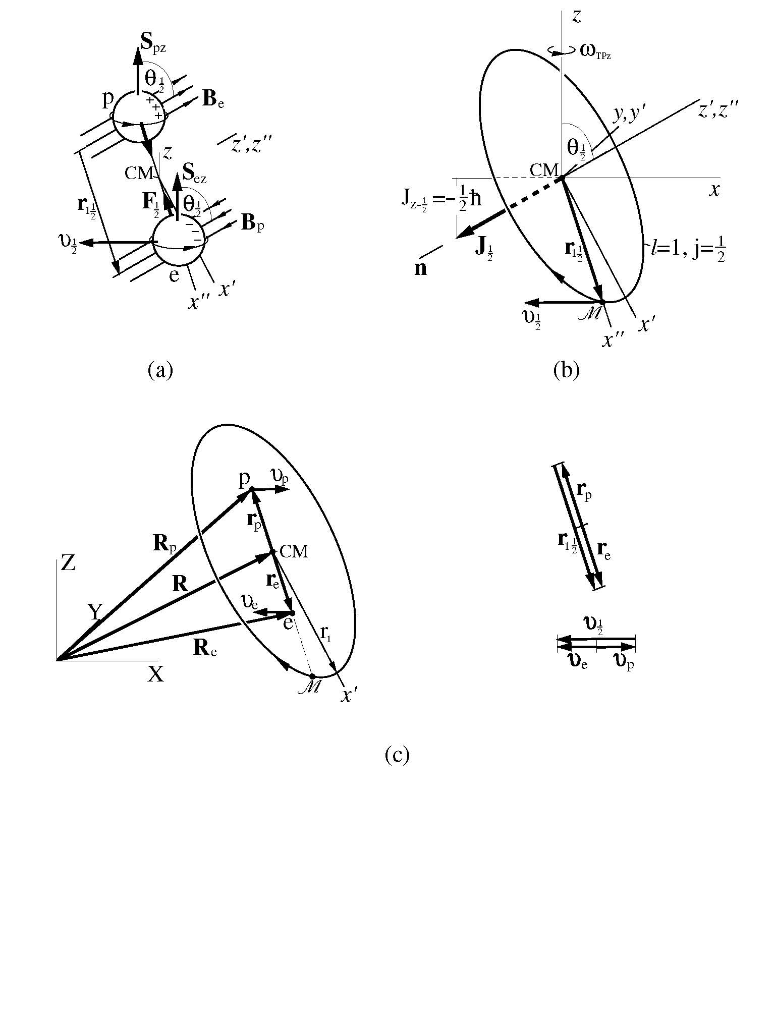
Figure 1: Schematic of the model neutron composed of an electron $e$ and a proton $p$. (a) The $e,p$ are separated by a distance ${\bf r}_{1{\mbox{\tiny{$\frac{1}{2}$}}}}=r_{1}\hat{r}_{1{\mbox{\tiny{$\frac{1}{2}$}}}}$ and are in relative angular motion and a Thomas precession at velocity ${\boldsymbol{\upsilon}}_{\mbox{\tiny{$\frac{1}{2}$}}}$ under a magnetic interaction force ${\bf{F}}_{{\mbox{\tiny{$\frac{1}{2}$}}}}$ in the magnetic fields ${\bf B}_{p},{\bf B}_{e}$ of $p,e$ at $e,p$; their spins ${\bf{S}}_{ez},{\bf{S}}_{pz}$ (in units $\hbar$) are aligned parallel, in the $+z$ direction for the $m_{j}=-j$ magnetic state shown, and antiparallel to $J_{z{\mbox{-}}{\mbox{\tiny{$\frac{1}{2}$}}}}$ of graph (b). (b) The reduced mass $\mathscr{M}$ of $e,p$ moves at velocity ${\boldsymbol{\upsilon}}_{\mbox{\tiny{$\frac{1}{2}$}}}$ about the CM along a $l=1,j=\frac{1}{2}$ circular orbit of radius vector ${\bf r}_{1{\mbox{\tiny{$\frac{1}{2}$}}}}$ and normal $\bf{n}$ at angle $\pi-\theta_{\mbox{\tiny{$\frac{1}{2}$}}}$ to the $z$ axis; it has a $z$-component angular momentum $J_{z{\mbox{-}}{\mbox{\tiny{$\frac{1}{2}$}}}}$. (c) Left: The $e,p$ are located at positions ${\bf r}_{e},{\bf r}_{p}$, moving at velocities ${\boldsymbol{\upsilon}}_{e},{\boldsymbol{\upsilon}}_{p}$, relative to the CM in the CM frame (coordinates $x,y,z$ in graph b), and at ${\bf{R}}_{e},{\bf{R}}_{p}$ in the lab frame (coordinates $X,Y,Z$). Right: vector relations between ${\bf r}_{e},{\bf r}_{p}$ and ${\bf r}_{1{\mbox{\tiny{$\frac{1}{2}$}}}}$, and ${\boldsymbol{\upsilon}}_{e},{\boldsymbol{\upsilon}}_{p}$ and ${\boldsymbol{\upsilon}}_{\mbox{\tiny{$\frac{1}{2}$}}}$. The drawings are made for $m_{e}\simeq m_{p}$.

Using several key relevant experimental facts, in particular the neutron beta decay reaction equation $n\rightarrow p+e+{\bar{\nu}}_{e}$, the neutron spin ($\frac{1}{2}$), the order of magnitude of the Fermi constant $G_{\mbox{{\tiny{$F$}}}}$ and the so implied weak interaction distance $\sim 1\cdot 10^{-18}$ m as direct input information, we propose at the outset of the theory development a real-space ($e,p$-) neutron model as follows: The neutron is composed of an electron $e$ and a proton $p$ separated at a distance $r(=r_{1})$ of an order $10^{-18}$ m; see Fig 1a. The $e,p$ are in relative orbital angular motion and in addition a Thomas precession at a velocity approaching the velocity of light $c$, under a central force of an electromagnetic origin. The central force is in effect predominantly an attractive magnetic force produced by the magnetic fields (${\bf B}_{p},{\bf B}_{e}$) of $p,e$ at $e,p$ as result of their intrinsic spin and relative motions. The $z$-components ($S_{ez}$, $S_{pz}$) of the $e,p$ spin angular momenta are aligned parallel to each other and antiparallel to that of their relative motion ($J_{z{\mbox{-}}{\mbox{\tiny{$\frac{1}{2}$}}}}$, Figs 1b), so that the magnetic interaction force is maximally attractive. The $e,p$ relative motion is in such a way that their reduced mass ($\mathscr{M}$) moves at a velocity (${\boldsymbol{\upsilon}}_{\mbox{\tiny{$\frac{1}{2}$}}}$) accordingly approaching $c$ along a (quantised $l=1,j=\frac{1}{2}$) circular orbit of radius $r(=r_{1})$ about their (the $e,p$) common centre of mass (CM), with a normal ($\bf{n}$) at a precession-modified quantised angle ($\pi-\theta_{\mbox{\tiny{$\frac{1}{2}$}}}$ for $j$ spin down state) to the $z$ axis; see Fig 1b. The relative precessional–orbital angular momentum projected in $z$ direction ($J_{z{\mbox{-}}{\mbox{\tiny{$\frac{1}{2}$}}}}$) will show to be a negative half-integer quantum $J_{z{\mbox{-}}{\mbox{\tiny{$\frac{1}{2}$}}}}=-\frac{1}{2}\hbar$. The corresponding neutral rotational energy flux, or vortex, along the $l=1,j=\frac{1}{2}$ circular orbit, of accordingly a $z$-component angular momentum $J_{z{\mbox{-}}{\mbox{\tiny{$\frac{1}{2}$}}}}$, resembles a ”confined antineutrino” (${\bar{\nu}}_{e}$).

It is commented that, the proposed $e,p$-neutron model suggests also a scheme for the strong force similarly on a unified basis with electromagnetism: A proton $p$ would be attracted with a neutron $n(e,p)$ (mainly) through an electrostatic attraction with the electron $e$ of the neutron at short range; in the same order of the short-range electrostatic interaction, two protons will repel, but never attract with one another. Such characteristics are in accordance with the observational fact that no nucleus exists which is made of more than one protons and protons only without neutrons. The author’s more recent research (internal work) has further shown that a microscopic representation of the muon and the ”muon-emitting” composite elementary particles may be achieved within a consistent scheme with the neutron model. The system of the so-represented elementary particles furthermore is in conformity with the quark model, in a manner that the (internal) spin states of the (composite) elementary particles are in one-to-one correspondences with the configurations of the (observationally-never-isolatable) quarks. The internal spin states of the model neutron under reversed signs (which represents the neutron effective spin, see Sec C), $-\frac{1}{2},-\frac{1}{2},\frac{1}{2}$ (i.e. ”down, down, up”), for example, directly correspond with the $ddu$ quarks. The (free) proton, as another example, is a non-composite particle with only one spin state, assigned as $+\frac{1}{2}$ (spin up) by convention. But this may be translated into a systematic three-spin states representation as $\frac{1}{2},\frac{1}{2},-\frac{1}{2}$ (i.e. ”up, up, down”), by adding two dummy spins $\frac{1}{2},-\frac{1}{2}$ without changing the original spin $\frac{1}{2}$; the three spin states correspond directly to the $uud$ quarks.

The remainder of this paper gives a first-principles mathematical representation of the model neutron, mainly in respect to the internal relativistic kinematics, dynamics (Secs B), magnetic structure (Sec C), and a derivation of the internal $e,p$ interaction force (Sec D) of the neutron in stationary state, the dynamics upon the neutron $\beta$ decay (Secs E), and a quantitative evaluation of the dynamical variables (Sec F). The (quantitative) predictions of the basic properties of the neutron are subsequently subjected to comparisons with, or constraints by, the available experimental data where in question, so that critical checks and controls of the viability of the neutron model are made as far as possible. Other basic aspects, including the parity associated with the $\beta$ decay, a direct derivation of the intermediate vector boson masses and Weinberg mixing angle of the neutron, and a corresponding dynamic scheme for the other (composite) elementary particles participating weak interaction, will be elucidated in separate papers.

Appendix B Equations of motion. Coordinate transformations. Solutions

B.1. Transformed Newtonian equations of motion of the mean and instantaneous positions of $e,p$. Representation in ${\bf r},{\bf{R}}$ coordinates Consider that an electron $e$ and a proton $p$ comprising a neutron are at time $t$ located with the probability densities $|\psi_{\alpha}({\bf{R}}_{\alpha},t)|^{2}$ ($\alpha=e,p$) at positions ${\bf{R}}_{e},{\bf{R}}_{p}$ relative to coordinates $X,Y,Z$ fixed in the laboratory (lab) frame; see Fig 1c. (The usual statistical point-particle picture suffices and is referred to here.) The $e,p$ are in relative motion at a velocity to prove high compared to $c$ (Sec F) under a mutual interaction force ${\bf{F}}$ and gravity ${\bf{g}}$; no applied force presents. Their mean positions, $\bar{{\bf{R}}}_{\alpha}=\int{\bf{R}}_{\alpha}|\psi_{\alpha}|^{2}d^{3}R_{\alpha}$, evolve according to the transformed Newtonian equations of motion, $\frac{d(m_{\alpha}(d\bar{{\bf{R}}}_{\alpha}/dt))}{dt}=\int(m_{\alpha}{\bf{g}}\pm{\bf{F}})|\psi_{\alpha}|^{2}d^{3}R_{\alpha}$ (the correspondence principle), where $m_{e},m_{p}$ are the $e,p$ masses. The $e,p$ are assumed to form a bound stationary system until Sec E and hence feasibly move circularly at constant (tangential) velocities (${\bf{u}}_{\alpha}=d{\bf{R}}_{\alpha}/dt$). The equations of motion thus reduce to

$$\halign{\hbox to\displaywidth{$\hfil\displaystyle#\hfil$}\cr 0.0pt{\hfil$\displaystyle\hfill m_{e}\frac{d^{2}{\bf{R}}_{e}}{dt^{{}2}}=m_{e}{\bf{g}}+{\bf{F}},\quad m_{p}\frac{d^{2}{\bf{R}}_{p}}{dt^{{}2}}=m_{p}{\bf{g}}-{\bf{F}}.\quad{\rm Or}\ \ M\frac{d^{2}{\bf{R}}}{dt^{{}2}}=M{\bf{g}},\quad{\mbox{$\mathscr{M}$}}\frac{d^{2}{\bf r}}{dt^{{}2}}={\bf{F}},\hfill(\ref{eq-EqMt})\cr 0.0pt{\hfil$\displaystyle{\rm where}\hfill\cr 0.0pt{\hfil$\displaystyle\hfill{\bf{R}}=\frac{m_{e}{\bf{R}}_{e}+m_{p}{\bf{R}}_{p}}{M},\ \ M=m_{e}+m_{p},\ \ {\bf r}{}={\bf{R}}_{e}-{\bf{R}}_{p}=\mathbf{r}_{e}-\mathbf{r}_{p},\ \ {\mbox{$\mathscr{M}$}}=\left(\frac{1}{m_{e}}+\frac{1}{m_{p}}\right)^{-1}=\frac{m_{e}m_{p}}{M};\hfill\cr 0.0pt{\hfil$\displaystyle\hfill{\bf{R}}_{e}={\bf{R}}+\frac{m_{p}}{M}{\bf r},\quad{\bf{R}}_{p}={\bf{R}}-\frac{m_{e}}{M}{\bf r};\quad\mathbf{r}_{e}={\bf{R}}_{e}-{\bf{R}}=\frac{m_{p}}{M}{\bf r},\quad\mathbf{r}_{p}={\bf{R}}_{p}-{\bf{R}}=-\frac{m_{e}}{M}{\bf r}.\hfill(\ref{eq-EqMt3})\crcr}}}}}$$

${\bf{R}}$ is the position of the centre of mass, CM; $M$ is the total mass located at ${\bf{R}}$; ${\bf r}$ is the relative position; $\mathscr{M}$ is the reduced mass (of a fictitious particle) located at ${\bf r}$; and $\mathbf{r}_{e},\mathbf{r}_{p}$ are the $e,p$ positions relative to ${\bf{R}}$. Eqs (Bc,d) are given for the masses $M$ and $\mathscr{M}$ travelling accordingly circularly at constant velocities (${\bf{u}}_{\mbox{{\tiny{cm}}}}=d{\bf{R}}/dt$ relative to the lab frame and ${\boldsymbol{\upsilon}}$ about the CM). A common time $t$ measured by a clock fixed at the CM has been used in order to facilitate the direct transformation of Eqs (Ba,b) to (Bc,d). Corresponding directly with the dynamic effect of $d^{2}{\bf{R}}_{\alpha}/dt^{2}$ on the left of Eqs (Ba,b), this $t$ enters as an independent variable of ${\bf{g}},{\bf{F}}$: ${\bf{g}}={\bf{g}}(t)$, ${\bf{F}}={\bf{F}}(t)$; the relativistic masses $m_{e},m_{p}$ may remain as (implicit) functions of the local times ($t_{e},t_{p}$) at ${\bf r}_{e},{\bf r}_{p}$ (Sec B.2) in so far as the same masses are used through the equations. For the $e,p$ relative motions internal of a neutron are of major concern in this paper, unless specified otherwise we shall work in the CM frame, i.e. immediately in terms of the relative positions ${\bf r}_{e},{\bf r}_{p},{\bf r}$ measured with respect to a set of relative coordinate axes $x,y,z$ parallel with the $X,Y,Z$ axes, and with an origin fixed at the CM (cf Fig 1b). This in more general terms means that we shall work with the unsuperscripted variables, including ${\bf{R}},M,{\bf{R}}_{e},m_{e},t$ etc, which we hereafter reserve to explicitly refer to ones measured in the CM frame. We shall refer to their counterparts for example measured in the lab frame by ${\bf{R}}^{\mbox{\tiny{lab}}},M^{\mbox{\tiny{lab}}},{\bf{R}}_{e}^{\mbox{\tiny{lab}}},m_{e}^{\mbox{\tiny{lab}}},t^{\mbox{\tiny{lab}}}$, etc. where in question.

The partial–relative and relative velocities of the $e,p$, and the corresponding rotational angular momenta in the CM frame, in terms of the time $t$, follow as

$$\halign{\hbox to\displaywidth{$\hfil\displaystyle#\hfil$}\cr 0.0pt{\hfil$\displaystyle\hfill{\boldsymbol{\upsilon}}_{e}=\frac{d\mathbf{r}_{e}}{dt}=\frac{m_{p}}{M}{\boldsymbol{\upsilon}},\quad{\boldsymbol{\upsilon}}_{p}=\frac{d\mathbf{r}_{p}}{dt}=-\frac{m_{e}}{M}{\boldsymbol{\upsilon}},\quad{\boldsymbol{\upsilon}}=\frac{d{\bf r}}{dt}={\boldsymbol{\upsilon}}_{e}-{\boldsymbol{\upsilon}}_{p};\hfill(\ref{eq-vs})\cr 0.0pt{\hfil$\displaystyle\hfill{\bf{J}}_{e}=\mathbf{r}_{e}\times(m_{e}{\boldsymbol{\upsilon}}_{e})=\frac{m_{p}}{M}{\bf{J}},\quad{\bf{J}}_{p}=\mathbf{r}_{p}\times(m_{p}{\boldsymbol{\upsilon}}_{p})=\frac{m_{e}}{M}{\bf{J}},\quad{\bf{J}}={\bf{J}}_{e}+{\bf{J}}_{p}={\bf r}\times({\mbox{$\mathscr{M}$}}{\boldsymbol{\upsilon}})\hfill(\ref{eq-Lddg})\crcr}}}$$

From the relations (Bg,h) between the distances ${\bf r}_{e},{\bf r}_{p}$ of $e,p$ to the CM, and ${\bf r}$ of $e$ to $p$ it follows that, by virtue how time in essence is defined, the local times $t_{e},t_{p}$ and the time $t$ for light to traverse the distances ${\bf r}_{e},{\bf r}_{p},{\bf r}$ at a constant velocity $c$ are related as $t_{e}=(m_{p}/M)t$, $t_{p}=(m_{e}/M)t$. The partial-relative velocities in terms of $t_{e},t_{p}$ are

$$\halign{\hbox to\displaywidth{$\hfil\displaystyle#\hfil$}\cr 0.0pt{\hfil$\displaystyle\hfill{\boldsymbol{\upsilon}}_{e}^{{}\prime}=d\mathbf{r}_{e}/dt_{e}={\boldsymbol{\upsilon}},\quad{\boldsymbol{\upsilon}}_{p}^{{}\prime}=d\mathbf{r}_{p}/dt_{p}=-{\boldsymbol{\upsilon}}.\quad\hfill(\ref{eq-velsp})\crcr}}$$

Denote $f_{t}(e)=\frac{t}{t_{e}}=\frac{|d{\bf r}_{e}/dt_{e}|}{|d{\bf r}_{e}/dt|}=\frac{\upsilon_{e}^{\prime}}{\upsilon_{e}}$. Substituting $t=f_{t}(e)t_{e}$ in (Ba), setting ${\bf{R}}=0$, we have $m_{e}\frac{d^{2}{\bf r}_{e}}{d(f_{t}^{2}(e)t^{2}_{e})}=m_{e}{\bf{g}}(t)+{\bf{F}}(t)$, or $m_{e}\frac{d^{2}{\bf r}_{e}}{dt^{2}_{e}}=m_{e}f_{t}^{2}(e){\bf{g}}(t)+f_{t}^{2}(e){\bf{F}}(t)=m_{e}{\bf{g}}(t_{e})+{\bf{F}}(t_{e})$, recovering the original form of (Ba) expressed by its local time $t_{e}$ provided ${\bf{F}}(t_{e})=f_{t}^{2}(e){\bf{F}}(t)$, ${\bf{g}}(t_{e})=f_{t}^{2}(e){\bf{g}}(t)$. Similarly a factor $f_{t}(p)=\frac{t}{t_{p}}=\frac{\upsilon_{p}^{\prime}}{\upsilon_{p}}$ will project (Bb) to its original form expressed in $t_{p}$. The same projection factors, in the form of geometric mean $f_{t}^{2}=(f_{t}^{2}(e)f_{t}^{2}(p))^{1/2}$, will be obtained through direct derivation of the magnetic force in Sec D.

B.2. Lorentz-Einstein transformations The instantaneous rest frame fixed to each rotating particle, $e$, $p$, $\mathscr{M}$ or $M$, may be regarded as an inertial frame for each differential rotation which is essentially linear. (For a complete macroscopic rotation, non-inertial frame effects present and will be included separately, see Eqs (B) vs (B) below and in turn Sec B.4). Subsequently, the differentials of the space and time coordinates ${\bf r}_{e}$, $t_{e}$; ${\bf r}_{p}$, $t_{p}$; ${\bf r}$, $t$; ${\bf{R}}$, $\bar{t}_{ep}$ in the CM frame, and their counterparts ${\bf r}_{e}^{\mbox{\tiny{$0$}}}$, $t_{e}^{\mbox{\tiny{$0$}}}$; ${\bf r}_{p}^{\mbox{\tiny{$0$}}}$, $t_{p}^{\mbox{\tiny{$0$}}}$; ${\bf r}^{\mbox{\tiny{$0$}}}$, $t^{\mbox{\tiny{$0$}}}$; ${\bf{R}}^{\mbox{\tiny{$0$}}}$, $\bar{t}_{ep}^{\mbox{\tiny{$0$}}}$ in the respective (instantaneous) rest frames are related by the Lorentz-Einstein transformations,

$$\halign{\hbox to\displaywidth{$\hfil\displaystyle#\hfil$}\cr 0.0pt{\hfil$\displaystyle\hfill\gamma{}_{e}(d{\bf r}_{e}-{\boldsymbol{\upsilon}}_{e}^{\prime}dt_{e})=d{\bf r}_{e}^{\mbox{\tiny{$0$}}},\ \ \gamma{}_{e}(dt_{e}-\frac{{\boldsymbol{\upsilon}}_{e}^{\prime}\cdot d{\bf r}_{e}}{{c^{\prime}}^{2}})=dt_{e}^{\mbox{\tiny{$0$}}};\ \ \gamma{}_{p}(d{\bf r}_{p}-{\boldsymbol{\upsilon}}_{p}^{\prime}dt_{p})=d{\bf r}_{p}^{\mbox{\tiny{$0$}}},\ \ \gamma{}_{p}(dt_{p}-\frac{{\boldsymbol{\upsilon}}_{p}^{\prime}\cdot d{\bf r}_{p}}{{c^{\prime}}^{2}})=dt_{p}^{\mbox{\tiny{$0$}}};\hfill\cr 0.0pt{\hfil$\displaystyle\hfill\gamma{}(d{\bf r}-{\boldsymbol{\upsilon}}dt)=d{\bf r}^{\mbox{\tiny{$0$}}},\ \ \gamma{}(dt-\frac{{\boldsymbol{\upsilon}}\cdot d{\bf r}}{c^{2}})=dt^{\mbox{\tiny{$0$}}};\ \ \gamma{}_{\mbox{{\tiny{M}}}}(d{\bf{R}}-{\boldsymbol{\upsilon}}_{\mbox{{\tiny{M}}}}d\bar{t}_{ep})=d{\bf{R}}^{\mbox{\tiny{$0$}}},\ \ \gamma{}_{\mbox{{\tiny{M}}}}(d\bar{t}_{ep}-\frac{{\boldsymbol{\upsilon}}_{\mbox{{\tiny{M}}}}\cdot d{\bf{R}}}{{c^{\prime}}^{2}})=d\bar{t}_{ep}^{\mbox{\tiny{$0$}}}\hfill(\ref{eq-Eq-transf-Ax2})\crcr}}}$$

where $\gamma{}_{\alpha}=(1-{\upsilon_{\alpha}^{\prime}}^{2}/c^{\prime}{}^{2})^{-1/2}$ ($\alpha=e,p$), $\gamma{}=(1-\upsilon^{2}/c^{2})^{-1/2}$, $\gamma{}_{\mbox{{\tiny{M}}}}=(1-\upsilon_{{\mbox{{\tiny{M}}}}}^{2}/c^{2})^{-1/2}$; $c^{\prime}=d{\bf r}_{\alpha_{pht}}/dt_{\alpha}=c=d{\bf r}_{pht}/dt$ is the light speed measured in the CM frame; $\gamma{}_{\mbox{{\tiny{M}}}},\gamma{}$ are the (effective) Lorentz factors of the fictitious particles of masses $M,{\mbox{$\mathscr{M}$}}$ moving effectively at the velocities ${\boldsymbol{\upsilon}}_{\mbox{{\tiny{M}}}},{\boldsymbol{\upsilon}}$, such that their dynamical consequence is the same as that due to the motions of $m_{e},m_{p}$ relative to the CM. In particular, ${\boldsymbol{\upsilon}}_{\mbox{{\tiny{M}}}}$ needs be thought of as the speed of the CM relative to the $e,p$, i.e. ${\boldsymbol{\upsilon}}_{\mbox{{\tiny{M}}}}=\frac{d{\bf{R}}}{d\bar{t}_{ep}}$ given in terms of a mean local time $\bar{t}_{ep}$ of $e,p$; the CM is not moving relative to itself.

Transformations from the scalar distances $r_{e},r_{p},R,r$ to $r_{e}^{\mbox{\tiny{$0$}}},r_{p}^{\mbox{\tiny{$0$}}},R^{\mbox{\tiny{$0$}}},r^{\mbox{\tiny{$0$}}}$ at fixed $t$ (hence $t_{e},t_{p},\bar{t}_{ep}$), from the time $t$ to $t^{\mbox{\tiny{$0$}}}$ at fixed ${\bf r}$, and from the CM-frame masses $m_{e},m_{p},M,{\mbox{$\mathscr{M}$}}$ to their respective rest-frame counterparts $m_{e}^{\mbox{\tiny{$0$}}},m_{p}^{\mbox{\tiny{$0$}}},M^{\mbox{\tiny{$0$}}}(=m_{e}^{\mbox{\tiny{$0$}}}+m_{p}^{\mbox{\tiny{$0$}}}),{\mbox{$\mathscr{M}$}}^{\mbox{\tiny{$0$}}}(=m_{e}^{\mbox{\tiny{$0$}}}m_{p}^{\mbox{\tiny{$0$}}}/M^{\mbox{\tiny{$0$}}})$ follow as

$$\halign{\hbox to\displaywidth{$\hfil\displaystyle#\hfil$}\cr 0.0pt{\hfil$\displaystyle\hfill\gamma{}_{e}r_{e}=r_{e}^{\mbox{\tiny{$0$}}},\quad\gamma{}_{p}r_{p}=r_{p}^{\mbox{\tiny{$0$}}},\quad\gamma{}_{\mbox{{\tiny{M}}}}R=R^{\mbox{\tiny{$0$}}},\quad\gamma{}r=r^{\mbox{\tiny{$0$}}};\quad\gamma{}t=t^{\mbox{\tiny{$0$}}};\hfill(\ref{eq-Sca-trans}.1)\cr 0.0pt{\hfil$\displaystyle\hfill m_{e}=\gamma{}_{e}m_{e}^{\mbox{\tiny{$0$}}},\quad m_{p}=\gamma{}_{p}m_{p}^{\mbox{\tiny{$0$}}},\quad M=m_{e}+m_{p}=\gamma{}_{\mbox{{\tiny{M}}}}M^{\mbox{\tiny{$0$}}},\quad{\mbox{$\mathscr{M}$}}=\gamma{}{\mbox{$\mathscr{M}$}}^{\mbox{\tiny{$0$}}}.\quad\hfill(\ref{eq-Sca-trans}.2)\crcr}}}$$

Using Eqs (B.2) for $m_{e},m_{p},M,{\mbox{$\mathscr{M}$}}$ in (Bb),(d) gives (B), and solving gives (B) below:

$$\halign{\hbox to\displaywidth{$\hfil\displaystyle#\hfil$}\cr 0.0pt{\hfil$\displaystyle\hfill\gamma{}_{\mbox{{\tiny{M}}}}M^{\mbox{\tiny{$0$}}}=\gamma{}_{e}m_{e}^{\mbox{\tiny{$0$}}}+\gamma{}_{p}m_{p}^{\mbox{\tiny{$0$}}},\quad\gamma{}_{\mbox{{\tiny{M}}}}\gamma{}=\gamma{}_{e}\gamma{}_{p};\quad{\rm or}\quad M^{\mbox{\tiny{$0$}}}=m_{e}^{\mbox{\tiny{$\dagger$}}}+m_{p}^{\mbox{\tiny{$\dagger$}}},\quad{\rm where}\hfill(\ref{eq-EqMt3-c-Y1}.1)\cr 0.0pt{\hfil$\displaystyle\hfill m_{e}^{\mbox{\tiny{$\dagger$}}}=\frac{m_{e}}{\gamma{}_{\mbox{{\tiny{M}}}}}=\gamma{}_{e}^{\mbox{\tiny{$\dagger$}}}m_{e}^{\mbox{\tiny{$0$}}},\ \ m_{p}^{\mbox{\tiny{$\dagger$}}}=\frac{m_{p}}{\gamma{}_{\mbox{{\tiny{M}}}}}=\gamma{}_{p}^{\mbox{\tiny{$\dagger$}}}m_{p}^{\mbox{\tiny{$0$}}},\quad\gamma{}_{e}^{\mbox{\tiny{$\dagger$}}}=\frac{\gamma{}_{e}}{\gamma{}_{\mbox{{\tiny{M}}}}},\ \ \gamma{}_{p}^{\mbox{\tiny{$\dagger$}}}=\frac{\gamma{}_{p}}{\gamma{}_{\mbox{{\tiny{M}}}}};\quad\gamma{}_{e}^{\mbox{\tiny{$\dagger$}}}\gamma{}_{p}^{\mbox{\tiny{$\dagger$}}}=\frac{\gamma{}_{e}\gamma{}_{p}}{\gamma{}_{\mbox{{\tiny{M}}}}{}^{2}}=\frac{\gamma{}}{\gamma{}_{\mbox{{\tiny{M}}}}}=\gamma{}^{\mbox{\tiny{$\dagger$}}}\hfill(\ref{eq-EqMt3-c-Y1}.2)\cr 0.0pt{\hfil$\displaystyle\cr 0.0pt{\hfil$\displaystyle\hfill\gamma{}_{e}=\frac{\gamma{}_{\mbox{{\tiny{M}}}}(M^{\mbox{\tiny{$0$}}}\pm K)}{2m_{e}^{\mbox{\tiny{$0$}}}},\quad\gamma{}_{p}=\frac{\gamma{}_{\mbox{{\tiny{M}}}}(M^{\mbox{\tiny{$0$}}}\mp K)}{2m_{p}^{\mbox{\tiny{$0$}}}},\quad K=\sqrt{(M^{\mbox{\tiny{$0$}}})^{2}-4m_{e}^{\mbox{\tiny{$0$}}}m_{p}^{\mbox{\tiny{$0$}}}\gamma{}^{\mbox{\tiny{$\dagger$}}}}.\hfill(\ref{eq-EqMt3-c-Y})\crcr}}}}}$$

For (B) to have real solutions requires $(M^{\mbox{\tiny{$0$}}})^{2}-4m_{e}^{\mbox{\tiny{$0$}}}m_{p}^{\mbox{\tiny{$0$}}}\gamma{}^{\mbox{\tiny{$\dagger$}}}\geq 0$, or $\gamma{}^{\mbox{\tiny{$\dagger$}}}\leq(\gamma{}^{\mbox{\tiny{$\dagger$}}})_{{\mbox{\tiny{max}}}}=(M^{\mbox{\tiny{$0$}}})^{2}/4m_{e}^{\mbox{\tiny{$0$}}}m_{p}^{\mbox{\tiny{$0$}}}=459.556,$ where $\gamma{}^{\mbox{\tiny{$\dagger$}}}=(\gamma{}^{\mbox{\tiny{$\dagger$}}})_{{\mbox{\tiny{max}}}}$ if $K=0$, in which case $\gamma{}_{e}=\gamma{}_{\mbox{{\tiny{M}}}}M^{\mbox{\tiny{$0$}}}/2m_{e}^{\mbox{\tiny{$0$}}}$, $\gamma{}_{p}=\gamma{}_{\mbox{{\tiny{M}}}}M^{\mbox{\tiny{$0$}}}/2m_{p}^{\mbox{\tiny{$0$}}}\simeq\frac{1}{2}\gamma{}_{\mbox{{\tiny{M}}}}$, $m_{e}=m_{p}$. In general $m_{e}$ and $m_{p}$ may not be equal. Let $m_{e}=km_{p}$; this combined with (Ba) gives $(m_{e}=)km_{p}=\gamma{}_{e}m_{e}^{\mbox{\tiny{$0$}}}=\frac{1}{2}\gamma{}_{\mbox{{\tiny{M}}}}(M^{\mbox{\tiny{$0$}}}+K)$. Dividing it by (Bb) times $m_{p}^{\mbox{\tiny{$0$}}}$, i.e. $(m_{p}=)\gamma{}_{p}m_{p}^{\mbox{\tiny{$0$}}}=\frac{1}{2}\gamma{}_{\mbox{{\tiny{M}}}}(M^{\mbox{\tiny{$0$}}}-K)$ gives (Ba,b), and re-arranging (Bc) gives (Bc) below,

$$\halign{\hbox to\displaywidth{$\hfil\displaystyle#\hfil$}\cr 0.0pt{\hfil$\displaystyle\hfill k=\frac{M^{\mbox{\tiny{$0$}}}+K}{M^{\mbox{\tiny{$0$}}}-K},\ \ {\rm or}\ \ K=\frac{(k-1)M^{\mbox{\tiny{$0$}}}}{k+1};\quad\gamma{}^{\mbox{\tiny{$\dagger$}}}=\frac{(M^{\mbox{\tiny{$0$}}})^{2}-K^{2}}{4m_{e}^{\mbox{\tiny{$0$}}}m_{p}^{\mbox{\tiny{$0$}}}}=\frac{k(M^{\mbox{\tiny{$0$}}})^{2}}{(k+1)^{2}m_{e}^{\mbox{\tiny{$0$}}}m_{p}^{\mbox{\tiny{$0$}}}}\hfill(\ref{eq-gamdag})\crcr}}$$

Substituting in these $k=m_{e}/m_{p}=1.3165$ from the solution for neutron magnetic moment (Sec C) gives $K=\frac{(1.3165-1)}{1.3165+1}938.78(3)=128.26(5)$ GeV, and $\gamma{}^{\mbox{\tiny{$\dagger$}}}=450.96(0)$. Eqs (Bg),(h) and (Ba),(b) for this case become ${\bf r}_{e}=\frac{{\bf r}}{k+1}=0.43{\bf r}$, ${\bf r}_{p}=-\frac{k{\bf r}}{k+1}=-0.57{\bf r}$; ${\boldsymbol{\upsilon}}_{e}=0.43{\boldsymbol{\upsilon}}$, ${\boldsymbol{\upsilon}}_{p}=-0.57{\boldsymbol{\upsilon}}$ (cf Fig. 1c, right graph). $k{>\atop\sim}1$ implies $\gamma{}_{e},\gamma{}_{p}>>1$.

Multiplying $\frac{\gamma{}_{e}m_{e}}{\gamma{}_{e}+1}$ to the quadratics of Eq (Ba), and $\frac{\gamma{}_{p}m_{p}}{\gamma{}_{p}+1}$ to that of (Bb), adding, we obtain on the left side the total kinetic energy $T_{e}+T_{p}$ of $e$,$p$ measured in the CM frame and in time $t$,

$$\halign{\hbox to\displaywidth{$\hfil\displaystyle#\hfil$}\cr 0.0pt{\hfil$\displaystyle\hfill(T_{e}+T_{p}\equiv)\frac{\gamma{}_{e}m_{e}\upsilon_{e}^{2}}{\gamma{}_{e}+1}+\frac{\gamma{}_{p}m_{p}\upsilon_{p}^{2}}{\gamma{}_{p}+1}=\left[\frac{\gamma{}_{e}m_{p}}{(\gamma{}_{e}+1)M}+\frac{\gamma{}_{p}m_{e}}{(\gamma{}_{p}+1)M}\right]{\mbox{$\mathscr{M}$}}\upsilon^{2}(\equiv T)\hfill(\ref{eq-Tinv}.1)\cr 0.0pt{\hfil$\displaystyle\hfill\mbox{for}\ \gamma{}_{e},\gamma{}_{p}>>1:\quad m_{e}\upsilon_{e}^{2}+m_{p}\upsilon_{p}^{2}={\mbox{$\mathscr{M}$}}\upsilon^{2}\hfill(\ref{eq-Tinv}.2)\crcr}}}$$

The right side of (B.1) or (B.2) expresses the kinetic energy $T$ of the reduced mass relative to the CM. Eq (B.1) or (B.2) expresses invariance of kinetic energy under the ${\bf r}_{e},{\bf r}_{p}$ to ${\bf r},{\bf{R}}$ coordinate transformation as described in the CM frame and in time $t$. Performing similar operations to Eqs (Ba,b) instead we obtain on the left side the total kinetic energy $T_{e}^{\prime}+T_{p}^{\prime}$ of $e$,$p$ measured in the CM frame but in their local times $t_{e},t_{p}$,

$$\halign{\hbox to\displaywidth{$\hfil\displaystyle#\hfil$}\cr 0.0pt{\hfil$\displaystyle\hfill(T_{e}^{\prime}+T_{p}^{\prime}\equiv)\frac{\gamma{}_{e}m_{e}}{\gamma{}_{e}+1}\upsilon_{e}^{\prime}{}^{2}+\frac{\gamma{}_{p}m_{p}}{\gamma{}_{p}+1}\upsilon_{p}^{\prime}{}^{2}=\left[\frac{\gamma{}_{e}m_{e}}{(\gamma{}_{e}+1)M}+\frac{\gamma{}_{p}m_{p}}{(\gamma{}_{p}+1)M}\right]M\upsilon^{2}(\equiv T^{\prime})\hfill(\ref{eq-Tinvp}.1)\cr 0.0pt{\hfil$\displaystyle\hfill\mbox{for}\ \gamma{}_{e},\gamma{}_{p}>>1:\quad m_{e}\upsilon_{e}^{\prime}{}^{2}+m_{p}\upsilon_{p}^{\prime}{}^{2}=M\upsilon^{2}\hfill(\ref{eq-Tinvp}.2)\crcr}}}$$

The right side of (B.1) or (B.2) represents in effect the kinetic energy $T^{\prime}$ of the total mass at the CM relative to the $e,p$ local space and time coordinates. Since $M>{\mbox{$\mathscr{M}$}}$, so $T_{e}^{\prime}+T_{p}^{\prime}>T_{e}+T_{p}$. The difference $(T_{e}^{\prime}+T_{p}^{\prime})-(T_{e}+T_{p})$ apparently represents a kinetic energy contribution from the non-inertial frame motion at ${\bf r}_{e},{\bf r}_{p}$ relative to the CM.

Unless specified otherwise we shall hereafter suppose for simplicity the $e,p$ system as a whole, i.e. its CM, to be at rest in the lab frame. Provided further setting the coordinate origins of the CM and lab frames the same, hence ${\bf{R}}=0$, the relativistic effects in the two frames are the same.

B.3. Total mass as measured in the lab frame. Neutron mass For the centre of mass CM of the $e,p$ system assumed at rest in the lab frame, naturally an observer in the lab frame will measure a rest total mass $M^{\mbox{\tiny{lab}}}=M^{\mbox{\tiny{$0$}}}=m_{e}^{\mbox{\tiny{$0$}}}+m_{p}^{\mbox{\tiny{$0$}}}$ of the model neutron. In more elaborate terms, a measurement of the neutron mass in the laboratory is typically made in a specified say $X$ direction over a macroscopic time interval $\Delta t$ which is $>>2\pi r/\upsilon$, the rotation period of $\mathscr{M}$ (Secs B.4, F). During $\Delta t$, ${\boldsymbol{\upsilon}}_{e},\upsilon_{p}$ explore all directions each with a zero average projection in the $X$ direction. Hence the relativistic augments in the masses of $e,p$ as measured along the instantaneous directions ${\boldsymbol{\upsilon}}_{e},\upsilon_{p}$ in the CM frame do not enter the mass $M^{\mbox{\tiny{lab}}}(=m_{e}^{\mbox{\tiny{lab}}}+m_{p}^{\mbox{\tiny{lab}}})$ measured in the lab frame. (This mass augment however evidently enters the interaction force or potential of Sec D, which has a constant magnitude so as to manifestly effectuate a bound $e,p$ in stationary state irrespective of the direction of the $e,p$ separation.)

A dually relevant example here is electron scattering by a target neutron. In respect to the internal dynamics of a target neutron, an incident electron $e$ travelling in a fixed direction is as a (moving) observer in the lab frame. The incident $e$ thus will see the rest (as contrasted to relativistic) masses of the $e,p$ of the neutron. Moreover, the $e,p$ of the neutron are fast rotating along circles of similar radii about their CM and thus about equally exposed to the incident $e$. So in terms of exposure frequency, the $e,p$ would equally probably scatter with the incident $e$, through electro and magnetic potentials and naturally at their contracted radii $a_{e},a_{p}$. The scattering potential from the proton $p$ of the neutron, on the other hand, would dominate because of its much heavier rest mass, which for the electrostatic part at least is attractive. Incidentally, the experimentally measured electron-neutron scattering length is negative and suggests an attractive scattering potential.

The (very large) $e,p$ interaction potential fields within the neutron, on the other hand, are liable to (considerably) modify the vacuum potential surrounding the $e,p$ charges; the effect would be particularly large given the $e,p$ separation distance $10^{-18}$ m (Sec F) here is comparable with the inter-vacuuon distance based on the ”vacuuonic vacuum structure”^a. This would consequently further modify the $e,p$ particles’ rest masses, in terms of the IED model^b, produced as their generating charges move through this modified vacuum. ($a,b$: see the author’s earlier published work). The above gives a qualitative account for the (order of MeV) larger neutron rest mass over the sum of the $e,p$ rest masses; this difference is relatively small and is ignored where in question throughout this paper.

B.4. Eigenvalue equations. Orbital and precessional angular momenta. Antineutrino In the absence of applied force and omitting the very weak gravity, $M$ is free and hence not directly subject to quantisation condition. We thus need only to establish the relativistic Schrödinger or Klein-Gordon equation (KGE) for the reduced mass $\mathscr{M}$, in terms of the spherical polar coordinates $r,\vartheta,\phi$ transformed directly from $x,y,z$. The KGE has the usual form $[((E_{tot})_{op}-V)^{2}-{{\mbox{$\mathscr{M}$}}^{\mbox{\tiny{$0$}}}}^{2}c^{4}-(p^{2})_{op}c^{2}]\psi_{tot}=0$, where $(E_{tot})_{op}-V={\mbox{$\mathscr{M}$}}c^{2}$; the associated non-inertial frame effect is not contained in it and will be included separately. Since the mass $\mathscr{M}$ under consideration is moving at velocity exceedingly close to $c$ such that its rest-mass energy is negligibly small compared to its kinetic energy (Sec F), more relevant here is the square-root (SQR) form of the KGE: $\mathcal{H}_{op}\psi=\mathcal{H}\psi$, where $\mathcal{H}_{op}=\left((E_{tot})_{op}-V\right)-{\mbox{$\mathscr{M}$}}^{\mbox{\tiny{$0$}}}c^{2}+V=\mathcal{T}_{op}+V$, and $\mathcal{T}_{op}={\mbox{$\mathscr{M}$}}c^{2}-{\mbox{$\mathscr{M}$}}^{\mbox{\tiny{$0$}}}c^{2}=(\gamma{}-1){\mbox{$\mathscr{M}$}}^{0}c^{2}=\frac{(\gamma{}-1)\gamma{}(p^{2})_{op}}{\gamma{}^{2}(\upsilon/c)^{2}{\mbox{$\mathscr{M}$}}}=\frac{\gamma{}(p^{2})_{op}}{(\gamma{}+1){\mbox{$\mathscr{M}$}}}$ (with $\gamma{}^{2}(\frac{\upsilon}{c})^{2}=\gamma{}^{2}-1$) are the Hamiltonian and kinetic energy operators associated with the kinetic motion of $\mathscr{M}$; $(p^{2})_{op}=(p_{r}^{2})_{op}+\frac{({\mathcal{J}}^{2})_{op}}{r^{2}}$; $(p_{r}^{2})_{op}$ and $({\mathcal{J}}^{2})_{op}$ are the squared radial and orbital angular momentum operators. For the $e$,$p$ interaction potential $V$ being central (Sec D), hence $V({\bf r})=V(r)$, the wave function of $\mathscr{M}$, $\psi(r,\vartheta,\phi)$, may be written as $\psi=\mathcal{R}(r)\mathcal{Y}(\vartheta,\phi)$. And the SQR-KGE separates into two eigenvalue equations,

$$\halign{\hbox to\displaywidth{$\hfil\displaystyle#\hfil$}\cr 0.0pt{\hfil$\displaystyle\hfill\left[-\frac{\gamma{}\hbar^{2}}{(\gamma{}+1){\mbox{$\mathscr{M}$}}r^{2}}\frac{\partial}{\partial r}(r^{2}\frac{\partial}{\partial r})+\frac{\gamma{}l(l+1)\hbar^{2}}{(\gamma{}+1){\mbox{$\mathscr{M}$}}r^{2}}+V(r)\right]\mathcal{R}(r)=\mathcal{H}\mathcal{R}(r)\hfill(\ref{eq-Sch1-R})\cr 0.0pt{\hfil$\displaystyle\hfill({\mathcal{J}}{}^{2})_{op}\mathcal{Y}{}(\vartheta{},\phi{})={\mathcal{J}}{}^{2}\mathcal{Y}{}(\vartheta{},\phi{}),\quad({\mathcal{J}}{}^{2})_{op}=-\hbar^{2}\left(\frac{\partial^{2}}{\partial\vartheta^{2}}+\cot\vartheta\frac{\partial}{\partial\vartheta}+\frac{1}{\sin^{2}\vartheta}\frac{\partial^{2}}{\partial\phi^{2}}\right).\hfill(\ref{eq-eignev-eqL2})\crcr}}}$$

(B) may be solved without $V(r)$ being explicitly known. The eigen functions are the spherical harmonics, $\mathcal{Y}_{l}^{m_{\mbox{\tiny{$l$}}}}=C_{{\mbox{\tiny{$l$}}}}^{m_{\mbox{\tiny{$l$}}}}P_{l}^{m_{\mbox{\tiny{$l$}}}}(\cos\vartheta)e^{im_{\mbox{\tiny{$l$}}}\phi}$. The square-root eigen values and their $z$ components are

$$\halign{\hbox to\displaywidth{$\hfil\displaystyle#\hfil$}\cr 0.0pt{\hfil$\displaystyle\hfill{\mathcal{J}}_{\mbox{\tiny{$l$}}}=|{\bf r}_{\mbox{\tiny{$l$}}}\times({\mbox{$\mathscr{M}$}}{\boldsymbol{\upsilon}}_{t}{}_{\mbox{\tiny{$l$}}})|=\sqrt{l(l+1)}\ \hbar,\ \ {\mathcal{J}}_{z{m}_{\mbox{\tiny{$l$}}}}={\mathcal{J}}_{\mbox{\tiny{$l$}}}\cos\vartheta_{m_{\mbox{\tiny{$l$}}}}={m}_{\mbox{\tiny{$l$}}}\hbar,\ \ l=0,\,1,\,\ldots;{m}_{\mbox{\tiny{$l$}}}=0,\,\ldots,\,\mp l.\ \hfill(\ref{eq-eigenLcal})\crcr}}$$

Based on the semiclassical expression ${\bf r}_{\mbox{\tiny{$l$}}}\times({\mbox{$\mathscr{M}$}}{\boldsymbol{\upsilon}}_{t}{}_{\mbox{\tiny{$l$}}})$, the particle of mass $\mathscr{M}$ in $l$th state executes an orbital angular motion along a circular orbit $l$ of radius vector ${\bf r}_{\mbox{\tiny{$l$}}}$ at a tangential velocity ${\boldsymbol{\upsilon}}_{t{\mbox{\tiny{$l$}}}}=d{\bf r}_{\mbox{\tiny{$l$}}}/dt=\boldsymbol{\omega{}}_{o}\times{\bf r}_{\mbox{\tiny{$l$}}}$, $\boldsymbol{\omega{}}_{o}={\bf r}_{\mbox{\tiny{$l$}}}\times{\boldsymbol{\upsilon}}_{t{\mbox{\tiny{$l$}}}}/r_{\mbox{\tiny{$l$}}}^{2}$; ${\bf r}_{\mbox{\tiny{$l$}}}\equiv{\bf r}_{n}$ for all $l(=0,1,\ldots,n-1)$ values of the same principal quantum number $n$. The normal of the orbital plane or the axis of rotation $\bf{n}_{o}$ passes through the CM and is at a quantised angle $\vartheta_{m_{\mbox{\tiny{$l$}}}}$ to the $z$ axis.

Owing to their having a finite acceleration ${\bf{\mbox{\sf{a}}}}_{\mbox{\tiny{$l$}}}=-|d^{2}{\bf r}_{\mbox{\tiny{$l$}}}/dt{}^{2}|({\bf r}_{\mbox{\tiny{$l$}}}/r_{\mbox{\tiny{$l$}}})$ in radial direction here, as a well-known non-inertial frame effect the $e,p$ in addition execute a Thomas precession (TP), with an instantaneous angular velocity denoted by $\boldsymbol{\omega{}}_{\mbox{{\tiny{$TP$}}}}$ and thus angular momentum ${\bf{J}}_{{\mbox{{\tiny{$TP$}}}}}=r_{\mbox{\tiny{$l$}}}^{2}{\mbox{$\mathscr{M}$}}\boldsymbol{\omega{}}_{\mbox{{\tiny{$TP$}}}}$. $\boldsymbol{\omega{}}_{\mbox{{\tiny{$TP$}}}}=\frac{\gamma{}^{2}}{(\gamma{}+1)}\frac{{\bf{\mbox{\sf{a}}}}_{\mbox{\tiny{$l$}}}\times{\boldsymbol{\upsilon}}_{t{\mbox{\tiny{$l$}}}}}{c{}^{2}}$ according to LH Thomas (1927), as may be alternatively derived directly based on (transformed) infinitesimal Newtonian inertial-frame and hence linear motion combined with acceleration in infinitesimal time (internal work). $\boldsymbol{\omega{}}_{\mbox{{\tiny{$TP$}}}}$ is in the instantaneous direction ${\bf{\mbox{\sf{a}}}}_{\mbox{\tiny{$l$}}}\times{\boldsymbol{\upsilon}}_{t{\mbox{\tiny{$l$}}}}\propto-{\bf r}_{\mbox{\tiny{$l$}}}\times{\boldsymbol{\upsilon}}_{t{\mbox{\tiny{$l$}}}}=-{\boldsymbol{\mathcal{J}}}_{{\mbox{\tiny{$l$}}}}/{\mbox{$\mathscr{M}$}}$, i.e. opposite to ${\boldsymbol{\mathcal{J}}}_{{\mbox{\tiny{$l$}}}}$, describing an instantaneous rotation in opposite sense to the orbital angular motion underlining ${\boldsymbol{\mathcal{J}}}_{{\mbox{\tiny{$l$}}}}$. For a quantum system as the bound $e,p$ here, the $z$ component of ${\bf{J}}_{\mbox{{\tiny{$TP$}}}}$, $J_{{\mbox{{\tiny{$TP$}}}}z}$, will be necessarily constrained such that both the space quantisation conditions (B) above and (B) below are met.

The total, precessional-orbital angular momentum $J_{\mbox{\tiny{$j$}}}=|{\boldsymbol{\mathcal{J}}}_{\mbox{\tiny{$l$}}}-{\bf{J}}_{{\mbox{{\tiny{$TP$}}}}}|$ and its $z$ component $J_{zm_{j}}={\mathcal{J}}_{zm_{\mbox{\tiny{$l$}}}}-J_{{\mbox{{\tiny{$TP$}}}}z}=J_{\mbox{\tiny{$j$}}}\cos\theta_{m_{j}}$ are given according to the quantum vector addition model as

$$\halign{\hbox to\displaywidth{$\hfil\displaystyle#\hfil$}\cr 0.0pt{\hfil$\displaystyle\hfill J_{\mbox{\tiny{$j$}}}=|{\bf r}_{{\mbox{\tiny{$l$}}}{\mbox{\tiny{$j$}}}}\times({\mbox{$\mathscr{M}$}}{\boldsymbol{\upsilon}}_{\mbox{\tiny{$j$}}})|=r_{\mbox{\tiny{$l$}}}{\mbox{$\mathscr{M}$}}\upsilon_{j}=\sqrt{j(j+1)}\ \hbar,\quad j=l-l_{\mbox{{\tiny{$TP$}}}}=0,\,\frac{1}{2},\,1,\,\frac{3}{2},\,\ldots\hfill(\ref{eq-Lzb}.1)\cr 0.0pt{\hfil$\displaystyle\hfill J_{z{m}_{j}}=J_{\mbox{\tiny{$j$}}}\cos\theta_{{m}_{j}}=\mp J_{{\mbox{\tiny{$j$}}}}\cos\theta_{{\mbox{\tiny{$j$}}}}={m}_{j}\hbar,\quad{m}_{j}=\mp j,\hfill(\ref{eq-Lzb}.2)\crcr}}}$$

where the permitted $j$ values are results of the general solutions of the quantum commutation relation for the angular momentum ${\mathbf{J}}$ here, ${\mathbf{J}}\times{\mathbf{J}}=i\hbar{\mathbf{J}}$. ${\bf r}_{{\mbox{\tiny{$l$}}}{\mbox{\tiny{$j$}}}}=r_{\mbox{\tiny{$l$}}}\hat{r}_{{\mbox{\tiny{$l$}}}{\mbox{\tiny{$j$}}}}$ is the quantised radius vector of the instantaneous circular orbit $l$ of a normal or axis of rotation $\bf{n}$; $\bf{n}$ is at a fixed angle $\theta_{m_{\mbox{\tiny{$j$}}}}=\arccos{(J_{zm_{\mbox{\tiny{$j$}}}}/J_{j})}$ to the $z$ axis and rotates about the $z$ axis at the angular velocity $\boldsymbol{\omega{}}_{{\mbox{{\tiny{$TP$}}}}z}$ in opposite sense to that of the $\omega{}_{o}$-orbital angular motion projected in the $xy$ plane, whence the Thomas precession; see Fig 1b. The magnitude of ${\bf r}_{{\mbox{\tiny{$l$}}}{\mbox{\tiny{$j$}}}}$, $|{\bf r}_{{\mbox{\tiny{$l$}}}{\mbox{\tiny{$j$}}}}|=r_{\mbox{\tiny{$l$}}}$ is unchanged subjected to the radial eigenvalue equation (B) but immediately to the quantum equation (Ba) here. ${\boldsymbol{\upsilon}}_{j}=d{\bf r}_{{\mbox{\tiny{$l$}}}{\mbox{\tiny{$j$}}}}/dt=\boldsymbol{\omega{}}\times{\bf r}_{{\mbox{\tiny{$l$}}}{\mbox{\tiny{$j$}}}}$; $\boldsymbol{\omega{}}={\bf r}_{{\mbox{\tiny{$l$}}}{\mbox{\tiny{$j$}}}}\times{\boldsymbol{\upsilon}}_{j}/r_{\mbox{\tiny{$l$}}}^{2}=|\boldsymbol{\omega{}}_{o}-\boldsymbol{\omega{}}_{{\mbox{{\tiny{$TP$}}}}}|\bf{n}$ is the precessional-orbital angular velocity. For facilitating later discussion we attach as in Fig 1b the axes $x^{\prime},y^{\prime},z^{\prime}$ to the instantaneous rest frame of the precessional orbit $l$, with their origin coinciding with that of $x,y,z$, i.e. fixed at the CM. So the $x^{\prime},y^{\prime},z^{\prime}$ axes precess about the $z$ axis at the angular velocity $\omega{}_{{\mbox{{\tiny{$TP$}}}}z}$, in counterclockwise sense for the $m_{j}=-j$ state in the figure, in such a way that the $z^{\prime}$ axis maintains at fixed angle $\theta_{j}$ to the $z$ axis, the $x^{\prime}$ axis at fixed angle $\theta_{j}$ to (its projection $x^{\prime}_{xy}$ in) the $xy$ plane and along the ${\bf r}_{{\mbox{\tiny{$l$}}}{\mbox{\tiny{$j$}}}}$ direction, and the $y^{\prime}$ axis in the $xy$ plane. And we attach the $x^{\prime\prime},y^{\prime\prime},z^{\prime\prime}$ axes to the instantaneous rest frame of the precessing-orbiting particles $e,p$ with an origin fixed at the CM too, the $z^{\prime\prime}$ axis coinciding with $z^{\prime}$, and the $x^{\prime\prime}$ axis lying along the line joining the $e,p$; see Fig 1a,b. So the $x^{\prime\prime},y^{\prime\prime}$ axes rotate in the $x^{\prime}y^{\prime}$ plane and about the $z^{\prime}$ ($z^{\prime\prime}$) axis, in clockwise sense for the $m_{j}=-j$ state, at the angular velocity $\omega{}_{o}+\omega{}_{\mbox{{\tiny{$TP$}}}}$ relative to the $x^{\prime},y^{\prime}$ axes.

From Eq (B.1b), it follows that the permitted $l_{\mbox{{\tiny{$TP$}}}}$ values are uniquely specified once $l,j$ are specified according to (B),(B): For $l=0$, only $l_{\mbox{{\tiny{$TP$}}}}=0$ is permitted; and $j=l=0$. This gives an $e,p$ system not magnetically bound at a separation of the order $10^{-18}$ m (see further Sec D); a bound system would in principle be obtainable at much larger separation as a hydrogen only. For any non-zero integer $l$ values, $l_{\mbox{{\tiny{$TP$}}}}=0$ is permitted formally by (B.1) but is however unphysical because of the so implied absence of Thomas precession. $l_{\mbox{{\tiny{$TP$}}}}=\frac{1}{2}$ is therefore the smallest finite and hence physical value which is also permitted based on the quantum solutions for $l,j$. Moreover, $l_{\mbox{{\tiny{$TP$}}}}=\frac{1}{2}$ is itself a solution for ${\bf{J}}_{{\mbox{{\tiny{$TP$}}}}z}$ to separately satisfy the quantum commutation relation ${\bf{J}}_{{\mbox{{\tiny{$TP$}}}}z}\times{\bf{J}}_{{\mbox{{\tiny{$TP$}}}}z}=i\hbar{\bf{J}}_{{\mbox{{\tiny{$TP$}}}}z}$; this establishes a condition for the carrier of ${\bf{J}}_{{\mbox{{\tiny{$TP$}}}}z}$, the neutral rotational energy flux (to be identified as the antineutrino) to be created or emitted as a quantum particle. Higher half-integer or integer $l_{\mbox{{\tiny{$TP$}}}}$ values satisfying (B.1) and (B) are permitted in theory but are not liable for a neutron candidate and will not be considered. For the permitted $l$ and $l_{\mbox{{\tiny{$TP$}}}}=\frac{1}{2}$, Eqs (B) are written as

$$\halign{\hbox to\displaywidth{$\hfil\displaystyle#\hfil$}\cr 0.0pt{\hfil$\displaystyle\hfill J_{\mbox{\tiny{$j$}}}=r_{\mbox{\tiny{$l$}}}{\mbox{$\mathscr{M}$}}\upsilon_{j}=\sqrt{j(j+1)}\,\hbar=\mbox{$\frac{\sqrt{(4l^{2}-1)}\ \hbar}{2}$},\quad\mbox{ $j=l-\frac{1}{2}=\frac{1}{2},\frac{3}{2},\ldots$};\hfill(\ref{eq-Lzb}.1)^{\prime}\cr 0.0pt{\hfil$\displaystyle\hfill J_{z{m}_{j}}=J_{\mbox{\tiny{$j$}}}\cos\theta_{m_{j}}={m}_{j}\hbar=(\mp|m_{\mbox{\tiny{$l$}}}|\pm\mbox{$\frac{1}{2}$})\hbar,\quad{m}_{\mbox{\tiny{$j$}}}=\mp j=\mp|m_{\mbox{\tiny{$l$}}}|\pm\mbox{$\frac{1}{2}$}=\mp\mbox{$\frac{1}{2}$},\ldots,\mp j,\hfill(\ref{eq-Lzb}.2)^{\prime}\crcr}}}$$

where $\cos\theta_{m_{\mbox{\tiny{$j$}}}}=\frac{J_{z{m}_{j}}}{J_{\mbox{\tiny{$j$}}}}=\frac{\mp 2l\pm 1}{\sqrt{4l^{2}-1}}$. For $j=\frac{1}{2}$, ${m}_{j}=\mp\frac{1}{2}$:

$$\halign{\hbox to\displaywidth{$\hfil\displaystyle#\hfil$}\cr 0.0pt{\hfil$\displaystyle\hfill J_{{\mbox{\tiny{$\frac{1}{2}$}}}}=|{\bf r}_{1{\mbox{\tiny{$\frac{1}{2}$}}}}\times({\mbox{$\mathscr{M}$}}{\boldsymbol{\upsilon}}_{\mbox{\tiny{$\frac{1}{2}$}}})|=r_{1}{\mbox{$\mathscr{M}$}}\upsilon_{\mbox{\tiny{$\frac{1}{2}$}}}=\mbox{$\frac{\sqrt{3}\ \hbar}{2}$},\quad J_{z\mp{\mbox{\tiny{$\frac{1}{2}$}}}}=r_{1}{\mbox{$\mathscr{M}$}}\upsilon_{\mbox{\tiny{$\frac{1}{2}$}}}\cos\theta_{\mp{\mbox{\tiny{$\frac{1}{2}$}}}}=\mp\mbox{$\frac{\hbar}{2}$};\hfill(\ref{eq-Lzb-p})\crcr}}$$

$\cos\theta_{\mbox{\tiny{$\frac{1}{2}$}}}=J_{z{\mbox{\tiny{$\frac{1}{2}$}}}}/J_{\mbox{\tiny{$\frac{1}{2}$}}}=1/\sqrt{3}$; $\theta_{\mbox{\tiny{$\frac{1}{2}$}}}=\arccos(1/\sqrt{3})=54.7^{o}$. The $j=\frac{1}{2}$ ($l=1$) states describe a ground-state neutron (Secs C, D). Eq (Ba) thus gives the $e,p$ relative precessional–orbital angular momentum internal of the neutron, and (Bb) the two possible $z$ components associated with a minimum-energy (${m}_{j}=-\frac{1}{2}$) and excitation (${m}_{j}=\frac{1}{2}$) state in an applied magnetic field in the $+z$ direction (see Sec C). The precessing circular orbit of the mass $\mathscr{M}$ has the quantised radius vector ${\bf r}_{1{\mbox{\tiny{$\frac{1}{2}$}}}}$ about the CM in the $x^{\prime}y^{\prime}$ plane. For the ${m}_{j}=-\frac{1}{2}$ state, the normal $\bf{n}$ of the rotation plane, and hence ${\mathbf{J}}_{{\mbox{\tiny{$\frac{1}{2}$}}}}$, is at angle $\theta_{{\mbox{-}}{\mbox{\tiny{$\frac{1}{2}$}}}}=\pi-\theta_{{\mbox{\tiny{$\frac{1}{2}$}}}}$ to the $z$ axis, the rotation being in clockwise sense, as shown in Fig 1b. And conversely for ${m}_{j}=\frac{1}{2}$. For the next orbital, $j=\frac{3}{2}$ ($l=2$), $J_{z\frac{3}{2}}/J_{\frac{3}{2}}=3/\sqrt{15}$, $\theta_{\frac{3}{2}}=39.2^{o}$.

For the neutron existing (in zero applied field) only in a single non-degenerate state $j=l-\frac{1}{2}=\frac{1}{2}$ and presuming that, in terms of the SQR-KGE here, energies of different $l$ and same $n$ are degenerate, then $N$ (the radial degree of freedom)$=0$ and $n=N+l+1=0+l+1=2$. So $\mathcal{T}_{r{\mbox{\tiny{$l$}}}}|_{{\mbox{\tiny{$l$}}}=n-1=1}=0$; and the total kinetic energy of $\mathscr{M}$ is, with $J_{\mbox{\tiny{$\frac{1}{2}$}}}^{2}(=({\boldsymbol{\mathcal{J}}}_{1}-{\bf{J}}_{{\mbox{{\tiny{$TP$}}}}})^{2})$ for ${\mathcal{J}}_{1}^{2}$ and $T$ in place of $\mathcal{T}$, $T_{\mbox{\tiny{$\frac{1}{2}$}}}=T_{t{\mbox{\tiny{$\frac{1}{2}$}}}}=\frac{\gamma{}}{(\gamma{}+1)}{\mbox{$\mathscr{M}$}}\upsilon_{{\mbox{\tiny{$\frac{1}{2}$}}}}^{2}=\frac{\gamma{}}{(\gamma{}+1)}(J_{{\mbox{\tiny{$\frac{1}{2}$}}}}^{2}/{\mbox{$\mathscr{M}$}}r_{1}^{2})=\frac{3\gamma{}\hbar^{2}M}{4(\gamma{}+1)m_{e}m_{p}r_{1}^{2}}$. Accordingly, the eigen energy (Hamiltonian) $H_{j}=T_{j}+V_{j}$, in place of $\mathcal{H}_{{\mbox{\tiny{$l$}}}=n-1}=\mathcal{T}_{{\mbox{\tiny{$l$}}}=n-1}+V_{{\mbox{\tiny{$l$}}}=n-1}$ (where $\mathcal{H}_{{\mbox{\tiny{$l$}}}=n-1}\equiv\mathcal{H}_{n}$, etc.), may be directly computed from the sum of the $T_{\mbox{\tiny{$j$}}}$ given above and the $V_{{\mbox{\tiny{$j$}}}}$ to be derived in Sec D, without formally solving the radial differential equation (B).

The precessional–orbital motion (propagation) of the $e,p$ particle waves $\psi_{e},\psi_{p}$ relative to one another, or alternatively of the matter wave $\psi$ of $\mathscr{M}$ relative to the CM, is associated with a neutral precessing-orbiting — simply rotational kinetic energy flux, or vortex, on disregarding their charges and also their rest-mass energies. This vortex entity carries a spin angular momentum with a $z$ component equal to one unit of half-integer quantum $J_{z\mp{\mbox{\tiny{$\frac{1}{2}$}}}}=\mp\frac{1}{2}\hbar$, has apparently a positive helicity, and therefore resembles directly an antineutrino (${\bar{\nu}}_{e}$) confined within the neutron; see further Sec E. Accordingly the $z$-component spin angular momenta of ${\bar{\nu}}_{e}$ are

$$\halign{\hbox to\displaywidth{$\hfil\displaystyle#\hfil$}\cr 0.0pt{\hfil$\displaystyle\hfill S_{{\bar{\nu}}_{e}z}=J_{z\mp{\mbox{\tiny{$\frac{1}{2}$}}}}=\mp\mbox{$\frac{1}{2}$}\hbar=\mp s_{{\bar{\nu}}_{e}}\hbar,\quad s_{{\bar{\nu}}_{e}}=\mbox{$\frac{1}{2}$}.\hfill(\ref{eq-Snubar})\crcr}}$$

Appendix C $e,p$ system magnetic structure. Neutron magnetic moment, (effective) spin

C.1 $e,p$ spins and magnetic moments. Neutron internal spin configurations. Total spin Either particle $\alpha=e$ or $p$ has an intrinsic spin $s_{\alpha}=\frac{1}{2}$, spin angular momentum $S_{\alpha}=\sqrt{s_{\alpha}(s_{\alpha}+1)}\ \hbar=\frac{\sqrt{3}}{2}\hbar$ about a spin axis $\bf{n}_{\alpha}$ passing through ${\bf r}_{\alpha}$, and $z$ component $S_{\alpha z}=S_{\alpha}\cos\theta^{s}_{\alpha}=\pm s_{\alpha}\hbar$. For the spin up state as in Fig 1a, $\cos\theta^{s}_{\alpha}=S_{\alpha z}/S_{\alpha}=1/\sqrt{3}$; the spin axis $\bf{n}_{\alpha}$ is at fixed angle $\theta^{s}_{\alpha}=54.73^{o}$ to a $z_{\alpha}^{s}$ axis parallel with $z$ and passing through ${\bf r}_{\alpha}$. Certain external, random environmental in the case of zero applied, magnetic field would always present and thus define the (instantaneous) $z$ direction here. For computing the magnetic field produced by the spin motion of one particle $\alpha$ at the other particle ($\alpha^{\prime}$), ${\bf B}_{\alpha}^{s}$ (Eq Db for $\alpha=p$, Sec D) at a separation $r_{\mbox{\tiny{$l$}}}$ comparable to the sizes of their charges (Secs. D, F), it is appropriate to treat the $e,p$ charges as extended objects, firstly simply as spheres of radii $a_{e},a_{p}$ with specific mass and charge distributions. We assume that the mass $m_{\alpha}$ of either particle $\alpha$ is distributed predominantly within its charge (and thus by a negligible amount in its wave field), with a volume density $\rho_{\alpha}(\boldsymbol{\xi}_{\alpha})$ at a distance $\boldsymbol{\xi}_{\alpha}$ from ${\bf r}_{\alpha}$; $dm_{\alpha}=m_{\alpha}\rho_{\alpha}(\boldsymbol{\xi}_{\alpha})d^{3}{\boldsymbol{\xi}_{\alpha}}$ is a mass element at $\boldsymbol{\xi}_{\alpha}$. So $S_{\alpha}$ formally is given rise to by the angular motion of the sphere about $\bf{n}_{\alpha}$ at the angular velocity $\omega{}^{s}_{\alpha}=d\phi_{\alpha}^{s}/dt_{\alpha}$, tangential velocity $\upsilon_{\alpha}^{s}=a_{\alpha}\omega{}^{s}_{\alpha}$ as,

$$\halign{\hbox to\displaywidth{$\hfil\displaystyle#\hfil$}\cr 0.0pt{\hfil$\displaystyle\hfill\mbox{ $S_{\alpha}=m_{\alpha}\int|\boldsymbol{\xi}_{\alpha}\times{\boldsymbol{\upsilon}}^{s}_{\alpha}|\rho_{\alpha}(\boldsymbol{\xi}_{\alpha})d^{3}{\boldsymbol{\xi}_{\alpha}}=\frac{1}{g_{\alpha}}a_{\alpha}^{2}\omega{}^{s}_{\alpha}m_{\alpha}=\frac{\sqrt{3}}{2}\ \hbar$};\quad S_{\alpha z}=\mbox{ $\frac{1}{g_{\alpha}}$}a_{\alpha}^{2}m_{\alpha}\omega{}^{s}_{\alpha}\cos\theta^{s}_{\alpha}=\mbox{ $\frac{1}{2}\hbar$}\hfill(\ref{eq-spinLs3})\crcr}}$$

where $g_{\alpha}$ is the Lande $g$ factor of particle $\alpha$. And the charge $q_{\alpha}$ of either particle $\alpha$ is distributed along a circular loop of radius $a_{\alpha}$ with a normal parallel with $\bf{n}_{\alpha}$. The spin (dipole) magnetic moment $\mu_{\alpha}^{s}$ of particle $\alpha$ is accordingly produced by the current loop of charge $q_{\alpha}$, area $\pi a_{\alpha}^{2}$, and angular velocity $\omega{}^{s}_{\alpha}$ in the $\mp S_{\alpha}$ direction for $q_{\alpha}=\mp e$. The $z$ components, written for $e,p$ explicitly, are

$$\halign{\hbox to\displaywidth{$\hfil\displaystyle#\hfil$}\cr 0.0pt{\hfil$\displaystyle\hfill\mu_{ez}^{s{}}=e\frac{\omega{}_{e}^{s{}}}{2\pi}\pi a_{e}^{2}\cos(\pi-\theta_{e}^{s{}})=-\frac{g_{e}eS_{ez}}{2m_{e}}=-\frac{g_{e}e\hbar}{4m_{e}};\quad\mu_{pz}^{s{}}=\frac{g_{p}eS_{pz}}{2m_{p}}=\frac{g_{p}e\hbar}{4m_{p}}\hfill(\ref{eq-muez})\crcr}}$$

For either particle $\alpha$, besides the $z_{\alpha}^{s}$ above we further specify the local axes $x_{\alpha}^{s},y_{\alpha}^{s}$ to be parallel with the $x,y$ but with an origin located at ${\bf r}_{\alpha}$. Its spin axis $\bf{n}_{\alpha}$ as projected in this $x_{\alpha}^{s}y_{\alpha}^{s}$ plane is unspecified in orientation according to the uncertainty principle, and in the external magnetic field in $z$ direction would rotate about the $z_{\alpha}^{s}$ axis. Accordingly the direction of ${\boldsymbol{\upsilon}}_{\alpha}^{s}{}$ at any fixed point on the current loop varies over time as the current loop precesses. Since the $z$ component $S_{\alpha z}$ of $S_{\alpha}$ is a constant (Eq Cb), the projection of ${\boldsymbol{\upsilon}}_{\alpha}^{s}$ in the $x_{\alpha}^{s}y_{\alpha}^{s}$ plane is a constant: $\upsilon^{s}_{\alpha_{xy}}=(a_{\alpha}\cos\theta^{s}_{\alpha})\omega{}^{s}_{\alpha}=\upsilon_{\alpha}^{s}\cos\theta^{s}_{\alpha}$; this gives also the time average of ${\boldsymbol{\upsilon}}_{\alpha}^{s}$, for the projection of ${\boldsymbol{\upsilon}}_{\alpha}^{s}$ in $z$ direction averages to zero over time. For deriving an effective algebraic equation for the magnetic field produced by the spin current loop (Sec D), the distinct symmetry property of the system will be utilised to further reduce the system to a two point half-charge representation (G).

C.2 $e,p$ system spin configuration. Total spin angular momentum For the $e,p$ to be in a bound, minimum (internal magnetic) energy state (Sec D), apart from the specific $j=\frac{1}{2}$ and $m_{j}=\mp\frac{1}{2}$ values (Sec B.4), $S_{ez},S_{pz}$ need be parallel mutually and each antiparallel to $J_{z{m}_{j}}$ (Figs 1a,b; 2a,b). $S_{ez},S_{pz},J_{z{m}_{j}}$ may therefore assume two possible configurations

$$\halign{\hbox to\displaywidth{$\hfil\displaystyle#\hfil$}\cr 0.0pt{\hfil$\displaystyle\hfill\mbox{$(i)\ \ S_{ez}=\frac{1}{2}\hbar,\ \ S_{pz}=\frac{1}{2}\hbar,\ \ J_{z{\mbox{-}}{\mbox{\tiny{$\frac{1}{2}$}}}}=-\frac{1}{2}\hbar;$}\quad\mbox{$(ii)\ \ S_{ez}=-\frac{1}{2}\hbar,\ \ S_{pz}=-\frac{1}{2}\hbar,\ \ J_{z{\mbox{\tiny{$\frac{1}{2}$}}}}=\frac{1}{2}\hbar$}\hfill(\ref{eq-anglmmtx1})\crcr}}$$

as shown in Figs 2a,b.

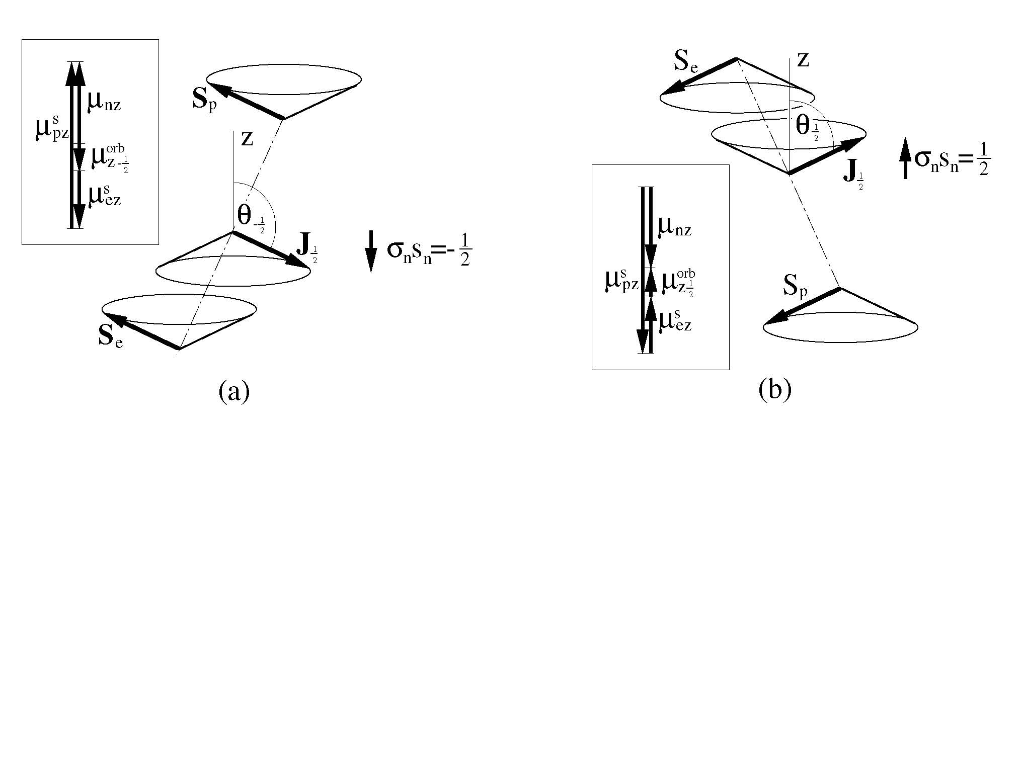
Figure 2: Internal angular momenta $S_{e},S_{p},J_{m_{j}}$ of the model neutron with the internal spin configurations (a) $s_{e},s_{p},m_{j}=\frac{1}{2},\frac{1}{2},-\frac{1}{2}$ in effective spin down state $s_{n}\sigma_{n}=m_{j}=-\frac{1}{2}$, and (b) $s_{e},s_{p},m_{j}=-\frac{1}{2},-\frac{1}{2},\frac{1}{2}$ in effective up state $\sigma_{n}s_{n}=m_{j}=\frac{1}{2}$. Insets in (a),(b): schematics of the corresponding $z$-component neutron magnetic moments $\boldsymbol{\mu}_{nz}$ as the respective vector sums of the internal component moments along $z$ direction.

Based on the usual vector addition model, the total angular momentum of the $e,p$ system, denoted by $\mbox{$\mathscr{J}$}_{{\mbox{\tiny{$j$}}}_{n}}$, in the precessional-orbital state $j=\frac{1}{2}$ are

$$\halign{\hbox to\displaywidth{$\hfil\displaystyle#\hfil$}\cr 0.0pt{\hfil$\displaystyle\hfill\mbox{$\mathscr{J}$}_{j_{n}}=\sqrt{j_{n}(j_{n}+1)}\hbar=\mbox{$\frac{\sqrt{3}}{2}\hbar$},\quad j_{n}=(s_{e}+s_{p})-j=(\frac{1}{2}+\frac{1}{2})-\frac{1}{2}=\frac{1}{2}\hfill(\ref{eq-totangm-z})\crcr}}$$

Its $z$ components $\mbox{$\mathscr{J}$}_{z{m}_{j_{n}}}$ for the $m_{j_{n}}=\pm j_{n}$ states are

$$\halign{\hbox to\displaywidth{$\hfil\displaystyle#\hfil$}\cr 0.0pt{\hfil$\displaystyle\hfill\mbox{$\mathscr{J}$}_{z\pm{\mbox{\tiny{$\frac{1}{2}$}}}}=(S_{pz}+S_{ez})_{{up\atop down}}+J_{z\mp{\mbox{\tiny{$\frac{1}{2}$}}}}\mbox{$=[\pm(\frac{1}{2}+\frac{1}{2})\mp\frac{1}{2}]\hbar=\pm\frac{1}{2}\hbar.$}\hfill(\ref{eq-totangm-zz})\crcr}}$$

C.3 Total magnetic moment The differing $g$ factors and potentially also asymmetric relative positions of $e,p$ suggest an asymmetric internal magnetic structure of the $e,p$ system. One thus expects a total magnetic moment which is not simply related to $\mbox{$\mathscr{J}$}_{zm_{j_{n}}}$ of Eqs (C) as for a simple particle; nor would it be zero as implied by its zero net charge as both given by the direct sum of the $e,p$ charges here and from experimental observation. We shall find the total magnetic moment based directly on vector addition of the individual magnetic moments along the $z$ direction below. For the spin configuration (i) of Eqs (C), the $z$-component total magnetic moment of the $e,p$ spins is the vector sum

$$\halign{\hbox to\displaywidth{$\hfil\displaystyle#\hfil$}\cr 0.0pt{\hfil$\displaystyle\hfill\mu^{s}_{z}=\mu_{pz}^{s}+\mu_{ez}^{s}=\frac{g_{p}eS_{pz}}{2m_{p}}-\frac{g_{e}eS_{ez}}{2m_{e}}=(g_{p}-\frac{g_{e}}{k})\frac{eS_{pz}}{2m_{p}},\hfill(\ref{eq-mun-1a})\crcr}}$$

where the last of Eqs (C) is given after substituting $m_{e}=km_{p}$ (as in Sec B.2) and $S_{ez}=S_{pz}$. $k$ may in general differ from 1. So the relative precessional-orbital motion may contribute a finite moment given by the vector sum, for the case (i) or $m_{j}=-\frac{1}{2}$,

$$\halign{\hbox to\displaywidth{$\hfil\displaystyle#\hfil$}\cr 0.0pt{\hfil$\displaystyle\hfill\mu_{z{\mbox{-}}{\mbox{\tiny{$\frac{1}{2}$}}}}^{orb}=\frac{eJ_{pz{\mbox{-}}{\mbox{\tiny{$\frac{1}{2}$}}}}}{2m_{p}}-\frac{eJ_{ez{\mbox{-}}{\mbox{\tiny{$\frac{1}{2}$}}}}}{2m_{e}}=\frac{e(\frac{m_{e}}{M})J_{z{\mbox{-}}{\mbox{\tiny{$\frac{1}{2}$}}}}}{2m_{p}}-\frac{e(\frac{m_{p}}{M})J_{z{\mbox{-}}{\mbox{\tiny{$\frac{1}{2}$}}}}}{2m_{e}}=\left(\frac{k-1}{k}\right)\frac{eJ_{z{\mbox{-}}{\mbox{\tiny{$\frac{1}{2}$}}}}}{2m_{p}}\hfill(\ref{eq-mun-2})\crcr}}$$

where $J_{\alpha zm_{j}}$ are the $z$-projections of $J_{\alpha j}$ given after Eqs (Ba,b); a $g$ factor equal to $1$ is assumed. The total $z$-component magnetic moment of the $e,p$ system is the vector sum

$$\halign{\hbox to\displaywidth{$\hfil\displaystyle#\hfil$}\cr 0.0pt{\hfil$\displaystyle\hfill\mu_{z{\mbox{-}}{\mbox{\tiny{$\frac{1}{2}$}}}\phi}=\mu_{z}^{s}+\mu_{z{\mbox{-}}{\mbox{\tiny{$\frac{1}{2}$}}}}^{orb}=(g_{p}-\frac{g_{e}}{k})\frac{e(-J_{z{\mbox{-}}{\mbox{\tiny{$\frac{1}{2}$}}}})}{2m_{p}}+\left(\frac{k-1}{k}\right)\frac{eJ_{z{\mbox{-}}{\mbox{\tiny{$\frac{1}{2}$}}}}}{2m_{p}}=-\frac{g_{n}eJ_{z{\mbox{-}}{\mbox{\tiny{$\frac{1}{2}$}}}}}{2m_{p}},\hfill(\ref{eq-mun-3}a)\cr 0.0pt{\hfil$\displaystyle\hfill g_{n}=g_{p}-\frac{g_{e}}{k}-\frac{k-1}{k}\hfill(\ref{eq-mun-3}b)\crcr}}}$$

where in the expression of $\mu_{z}^{s}$ we substituted $S_{pz}=-J_{z{\mbox{-}}{\mbox{\tiny{$\frac{1}{2}$}}}}$; $J_{zm_{j}}$, instead of $\mbox{$\mathscr{J}$}_{zm_{j_{n}}}$, is used for reason to be explained below. The subscript $\phi$ indicates that the total $\mu_{z{\mbox{-}}{\mbox{\tiny{$\frac{1}{2}$}}}\phi}$, as the $\mu_{pz}^{s}$, $\mu_{ez}^{s}$ and $\mu_{z{\mbox{-}}{\mbox{\tiny{$\frac{1}{2}$}}}}^{orb}$, is as directly probed by a detector placed at the CM relative to which the $e,p$ are moving in the ${\boldsymbol{\upsilon}}_{e},{\boldsymbol{\upsilon}}_{p}$ or $\phi$ directions, in which case the relativistic masses $m_{e},m_{p}$ in Eq (Ca) remain physical.

An experimenter (as an external observer) in the laboratory on the other hand commonly probes the neutron magnetic moment by applying a magnetic field to turn the moment along the $\theta$ direction, typically at a speed $u_{\theta}<<c$. This is to turn the $e,p$ system as a whole here, or manifestly the $e,p$ precessional-orbital plane about the $y^{\prime}$ axis along the $\theta$ direction in the $x^{\prime}z^{\prime}$ plane, i.e. in a direction perpendicular to ${\boldsymbol{\upsilon}}_{e},{\boldsymbol{\upsilon}}_{p}$. So immediately for the proton $\gamma{}_{p\theta}=(1-u_{p\theta}^{2}/c^{2})^{-1/2}\simeq 1$, $m_{p}(u_{p\theta})=\gamma{}_{p\theta}m_{p}^{\mbox{\tiny{$0$}}}\simeq m_{p}^{\mbox{\tiny{$0$}}}$; the proton dominates the turning process because of its much larger rest-mass moment of inertia. The electron can only be turned in the same rigid precessional-orbital plane as the proton in a bound relativistic dynamic process, its mass (hence moment of inertia) must therefore manifestly be weighed by the same factor $k$ as in this relativistic process, i.e. as $m_{e}=km_{p}$, not as $m_{e}^{\mbox{\tiny{$0$}}}$. The only means of correctly carrying the factor $k$ through to the experimenter’s result (Eq C below) is to convert $m_{e}$ to $km_{p}$ before transforming to Eq (C), as has been done in (Ca). Substituting $m_{p}^{\mbox{\tiny{$0$}}}$ in place of $m_{p}$ in the last of Eqs (Ca), and accordingly $\mu_{z{\mbox{-}}{\mbox{\tiny{$\frac{1}{2}$}}}}$ in place of $\mu_{z{\mbox{-}}{\mbox{\tiny{$\frac{1}{2}$}}}\phi}$, gives therefore the $z$-component magnetic moment of the model neutron, $\mu_{nz}$, as probed by the experimenter, for the $m_{j}=-\frac{1}{2}$ state

$$\halign{\hbox to\displaywidth{$\hfil\displaystyle#\hfil$}\cr 0.0pt{\hfil$\displaystyle\hfill\mu_{nz}(\mbox{$m_{j}=-\frac{1}{2}$})=\mu_{z{\mbox{-}}{\mbox{\tiny{$\frac{1}{2}$}}}}=-\frac{g_{n}eJ_{z{\mbox{-}}{\mbox{\tiny{$\frac{1}{2}$}}}}}{2m_{p}(u_{p\theta})}=-\frac{g_{n}eJ_{z{\mbox{-}}{\mbox{\tiny{$\frac{1}{2}$}}}}}{2m_{p}^{\mbox{\tiny{$0$}}}}=\frac{g_{n}e\hbar}{4m_{p}^{\mbox{\tiny{$0$}}}}=\frac{1}{2}g_{n}\mu_{{\mbox{\tiny${N}$}}},\hfill(\ref{eq-mu-4})\crcr}}$$

where $\mu_{{\mbox{\tiny${N}$}}}=\frac{e\hbar}{2m_{p}^{\mbox{\tiny{$0$}}}}$ (the nuclear magneton). Similarly for the $m_{j}=\frac{1}{2}$ state we obtain $\mu_{nz}(m_{j}=\frac{1}{2})=\mu_{z{\mbox{\tiny{$\frac{1}{2}$}}}}=-g_{n}eJ_{z{\mbox{\tiny{$\frac{1}{2}$}}}}/2m_{p}^{\mbox{\tiny{$0$}}}=-\frac{1}{2}g_{n}\mu_{{\mbox{\tiny${N}$}}}$. $g_{n}$ represents the $g$ factor of the model neutron. Equating $g_{n}$ of (Cb) with the experimental value $g_{n}^{exp}=3.8261$, and using the experimental $g$ values of $e,p$, $g_{p}=5.5857$, $g_{e}=2$, numerical solution for $k$ is obtained as $k=1.3165$. According to (C) or (Ca), $\mu_{z{\mbox{-}}{\mbox{\tiny{$\frac{1}{2}$}}}}>0$, i.e. $\mu_{z{\mbox{-}}{\mbox{\tiny{$\frac{1}{2}$}}}}$ points in the $+z$ direction, and is in the opposite direction to $J_{z{\mbox{-}}{\mbox{\tiny{$\frac{1}{2}$}}}}$ (Fig 2a). And $\mu_{z{\mbox{\tiny{$\frac{1}{2}$}}}}<0$ (Fig 2b). Clearly, the magnetic moment of the model neutron is dominated by the proton spin magnetic moment because of the asymmetrically much larger $g_{p}$ over $g_{e}$. From $k>1$ and hence $m_{e}>m_{p}$, $r_{p}>r_{e}$ (by a small amount each), it follows that $\mu_{z{\mbox{-}}{\mbox{\tiny{$\frac{1}{2}$}}}}^{orb}$ points in the $-z$ direction, adding a negative but small term to $\mu_{z{\mbox{-}}{\mbox{\tiny{$\frac{1}{2}$}}}}$.

C.4 Effective spin of the neutron In an applied magnetic field say ${\bf B}_{0}$ in $+z$ direction, the magnetic-interaction energy of the $e,p$ system with the field is $U_{j}=-\boldsymbol{\mu}_{j}\cdot{\bf B}_{0}=-\mu_{zm_{j}}B_{0}$. $U_{j}<0$ for the spin configuration (i) of Eqs (C) or the $m_{j}=-\frac{1}{2}$ state, and $U_{j}>0$ for (ii) or the $m_{j}=\frac{1}{2}$ state. That is, (i) or $m_{j}=-\frac{1}{2}$ corresponds to the minimum-energy state and (ii) or $m_{j}=\frac{1}{2}$ the excited state in the applied field. A transition from the minimum-energy to excited state corresponds to a flip of the spin-configuration (i) to (ii) of the bound $e,p$ system as a whole, which is dictated, and thus manifested by the flip of the processional-orbital plane from the $m_{j}=-\frac{1}{2}$ state to $m_{j}=+\frac{1}{2}$. In other terms, $\mu_{z_{{\mbox{-}}{\mbox{\tiny{$\frac{1}{2}$}}}}}$ is as if produced by a negative charged current loop in spin up state, or alternatively by a positively charged current loop in spin down state. In so far as the total magnetic moment of the $e,p$ system as a whole, whence the model neutron, is probed, it is therefore physical to assign to it an effective spin $s_{n}$ and spin vector $\sigma_{n}$, corresponding directly to the $j$ and $m_{j}=\mp j$ values (rather than the $j_{n}$ and $m_{j_{n}}$). So the effective neutron spin angular momentum $S_{n}$, its $z$ components $S_{nz}$, and accordingly $\mu_{zm_{j}}$ in relation with $S_{nz}$, given by substituting $S_{nz}$ for $J_{zm_{j}}$ in (C), are

$$\halign{\hbox to\displaywidth{$\hfil\displaystyle#\hfil$}\cr 0.0pt{\hfil$\displaystyle\hfill S_{n}=\sqrt{s_{n}(s_{n}+1)}\hbar\equiv J_{j}=\frac{\sqrt{3}}{2}\hbar,\quad s_{n}=j=\frac{1}{2};\quad S_{nz}=\sigma_{n}s_{n}\hbar\equiv J_{z_{m_{j}}}=m_{j}\hbar=\mp\frac{1}{2}\hbar,\hfill\cr 0.0pt{\hfil$\displaystyle\hfill\sigma_{n}=\mp 1\mbox{ (for $m_{j}=\mp\frac{1}{2}$});\quad\mu_{nz}=-\frac{g_{n}eS_{nz}}{2m_{p}^{\mbox{\tiny{$0$}}}}=-\frac{g_{n}\sigma_{n}s_{n}e\hbar}{2m_{p}^{\mbox{\tiny{$0$}}}}\equiv\mu_{z_{m_{j}}}=\pm\frac{g_{n}e\hbar}{4m_{p}^{\mbox{\tiny{$0$}}}}\hfill(\ref{eq-sn})\crcr}}}$$

Notice that for either spin configuration the $S_{n}$, $S_{nz}$ are equal to $\mbox{$\mathscr{J}$}_{j_{n}}$, $\mbox{$\mathscr{J}$}_{zm_{j_{n}}}$ in magnitudes but opposite in directions. The magnitude of $S_{n}$ or $\mbox{$\mathscr{J}$}_{zm_{j_{n}}}$, being a one-half integer quantum, has the absolute significance that it identifies the neutron as a fermion in accordance with observation. The assignment of the effective spin parameters $s_{n},\sigma_{n}$ above is in direct conformity with the role of the Standard Model neutron spin with respect to the experimental determination of neutron magnetic monument based on magnetic resonance method [1f].

Appendix D $e,p$ electromagnetic interaction. Weak interaction force

We shall below derive for the electron $e$ and proton $p$ comprising the model neutron in stationary state their interaction force ${\mathbf{F}}$, the corresponding potential $V$ and Hamiltonian $H$ based on first principles laws of electromagnetism and (the solutions of Sec B of) relativistic kinematics and quantum-mechanics. We shall continue to work in the CM frame, i.e. in terms of the unsuperscripted mass and space-time variables which will directly enter the electromagnetic interactions below, and for simplicity the time $t$ instead of $t_{e},t_{p}$; the local time $t_{e},t_{p}$ effect will be included in the end by a projecting factor ($f_{t}^{2}$). In this section, ${\bf r}$ or ${\bf r}_{{\mbox{\tiny{$l$}}}{\mbox{\tiny{$j$}}}}$ refers to the $e,p$ separation distance starting at ${\bf r}_{p}$, ending at ${\bf r}_{e}$, as in Figs 1a, c; its magnitude is equal to that of ${\bf r}$ or ${\bf r}_{{\mbox{\tiny{$l$}}}{\mbox{\tiny{$j$}}}}$ of Sec B.4, Fig 1b.

Consider the $e,p$ system in a precessional-orbital state $j=l-l_{\mbox{{\tiny{$TP$}}}}$, $m_{j}=-j$, with the $e,p$ spins $S_{pz}$, $S_{ez}$ in the $+z$ direction, i.e. antiparallel with $J_{z{\mbox{-}}j}$ (as in Figs 1a,b or Fig 2a for $j=1-\frac{1}{2}=\frac{1}{2}$, $m_{j}=-\frac{1}{2}$). Firstly, the proton of a charge $+e$ produces at the electron at ${\bf r}_{{\mbox{\tiny{$l$}}}{\mbox{\tiny{$j$}}}}$ apart a (transformed) Coulomb field ${\mathbf{E}}_{p}(r_{\mbox{\tiny{$l$}}})=(e/4\pi\epsilon_{0}r^{2}_{\mbox{\tiny{$l$}}})\ \hat{{\bf r}}_{{\mbox{\tiny{$l$}}}{\mbox{\tiny{$j$}}}}$ (in SI units here and below); $\hat{r}_{{\mbox{\tiny{$l$}}}{\mbox{\tiny{$j$}}}}={\bf r}_{{\mbox{\tiny{$l$}}}{\mbox{\tiny{$j$}}}}/r_{\mbox{\tiny{$l$}}}$ is a unit vector pointing from $p$ to $e$. $|{\mathbf{E}}_{p}|$ is amplified from its rest-frame value $E^{\mbox{\tiny{$0$}}}_{p}$ by a factor $\propto(1/r^{2})/(1/(r^{\mbox{\tiny{$0$}}})^{2})=\gamma{}^{2}=1/f_{c}$ and hence has a narrowed profile at a point ${\bf r}$ perpendicular to its motion $\phi$ direction by an inverse factor, $f_{c}$. And so are the magnetic fields below. Furthermore, the proton is in relative precessional–orbital motion in clockwise sense at the tangential velocity ${\boldsymbol{\upsilon}}_{p}$ about the CM in the $x^{\prime}y^{\prime}$ plane, and in spin motion at the tangential velocity ${\boldsymbol{\upsilon}}_{p_{xy}}^{s}$ in the $x_{p}^{s}y_{p}^{s}$ plane (Sec C.1). The latter, after a projection on to the $x^{\prime}y^{\prime}$ and hence $x^{\prime\prime}y^{\prime\prime}$ plane, may be effectively represented (Eq G, G) as two point half-charges located at $-\bar{\hskip 2.84544pta},\bar{\hskip 2.84544pta}$ from ${\bf r}_{p}$ on the $x^{\prime\prime}$ axis and moving oppositely at velocities $-\bar{\bf{\upsilon}}_{p}^{s}{}^{\prime\prime},+\bar{\bf{\upsilon}}_{p}^{s}{}^{\prime\prime}$ in $-y^{\prime\prime},+y^{\prime\prime}$ directions. So $p$ produces at $e$ magnetic fields ${\mathbf{B}}_{p}^{{orb}{}}(=-{\boldsymbol{\upsilon}}_{p}\times{\mathbf{E}}_{p}/c^{2})$ and ${\mathbf{B}}_{p}^{s{}}(r_{\mbox{\tiny{$l$}}}\pm\bar{\hskip 2.84544pta})(=\pm|\bar{\bf{\upsilon}}_{p}^{s}{}^{\prime\prime}\times{\mathbf{E}}_{p}(r_{\mbox{\tiny{$l$}}}\pm\bar{\hskip 2.84544pta})|/c^{2})$ along the $z^{\prime}$ direction given as (the transformed Biot-Savart law),

$$\halign{\hbox to\displaywidth{$\hfil\displaystyle#\hfil$}\cr 0.0pt{\hfil$\displaystyle\hfill{\bf B}^{orb{}}_{p}(r_{\mbox{\tiny{$l$}}},\theta_{j})=\frac{e{\boldsymbol{\upsilon}}_{p}\times{\bf r}_{{\mbox{\tiny{$l$}}}{\mbox{\tiny{$j$}}}}}{4\pi\epsilon_{0}c^{2}r_{\mbox{\tiny{$l$}}}^{3}}=-\frac{e{\bf r}_{{\mbox{\tiny{$l$}}}{\mbox{\tiny{$j$}}}}\times(-\frac{m_{e}m_{p}}{M}){\boldsymbol{\upsilon}}_{\mbox{\tiny{$j$}}}}{4\pi\epsilon_{0}m_{p}c^{2}r_{\mbox{\tiny{$l$}}}^{3}}=-\frac{\sqrt{4l^{2}-1}\ e\hbar\ \hat{z}^{\prime}}{8\pi\epsilon_{0}m_{p}c^{2}r_{\mbox{\tiny{$l$}}}^{3}};\hfill(\ref{eq-Bp1orb})\cr 0.0pt{\hfil$\displaystyle\hfill{\mathbf{B}}_{p}^{s{}}(r_{\mbox{\tiny{$l$}}}\pm\bar{\hskip 2.84544pta},\theta_{j})=\frac{\mp\frac{1}{2}e\bar{\boldsymbol{\upsilon}}_{p}^{s}{}^{\prime\prime}\times({\bf r}_{{\mbox{\tiny{$l$}}}{\mbox{\tiny{$j$}}}}/r_{\mbox{\tiny{$l$}}})}{4\pi\epsilon_{0}c^{2}(r_{\mbox{\tiny{$l$}}}\pm\bar{\hskip 2.84544pta})^{2}},\quad{\mathbf{B}}_{p}^{s}(r_{\mbox{\tiny{$l$}}},\theta_{j})={\mathbf{B}}_{p}^{s{}}(r_{\mbox{\tiny{$l$}}}-\bar{\hskip 2.84544pta},\theta_{j})+{\mathbf{B}}_{p}^{s{}}(r_{\mbox{\tiny{$l$}}}+\bar{\hskip 2.84544pta},\theta_{j})=\hfill\cr 0.0pt{\hfil$\displaystyle\hfill=\frac{e\bar{\hskip 2.84544pta}\bar{\boldsymbol{\upsilon}}_{p}^{s}{}^{\prime\prime}\times({\bf r}_{{\mbox{\tiny{$l$}}}{\mbox{\tiny{$j$}}}}/r_{\mbox{\tiny{$l$}}})}{2\pi\epsilon_{0}c^{2}r^{3}_{\mbox{\tiny{$l$}}}(1-\frac{\bar{\hskip 2.84544pta}^{2}}{r^{2}_{\mbox{\tiny{$l$}}}})^{2}}=\frac{-\eta^{2}g_{p}e\hbar\cos\theta_{\mbox{\tiny{$j$}}}\hat{z}^{\prime}}{4\pi\epsilon_{0}m_{p}c^{2}r{}^{3}_{\mbox{\tiny{$l$}}}C_{1{\mbox{\tiny{$l$}}}}},\quad C_{1{\mbox{\tiny{$l$}}}}\mbox{$=\left(1-\frac{\bar{\hskip 2.84544pta}^{2}}{r^{2}_{\mbox{\tiny{$l$}}}}\right)^{2}$}\hfill(\ref{eq-Bp1b})\crcr}}}}$$

The last of Eqs (D) is given after substituting (Bb) for ${\boldsymbol{\upsilon}}_{p}$ and (B.1)^′ for ${\bf r}_{{\mbox{\tiny{$l$}}}{\mbox{\tiny{$j$}}}}\times(\frac{m_{e}m_{p}}{M}){\boldsymbol{\upsilon}}_{\mbox{\tiny{$j$}}}$, given for $l_{\mbox{{\tiny{$TP$}}}}=\frac{1}{2}$. The last of Eqs (Db) is given after substituting (Ga), (Gb) for $\bar{\hskip 2.84544pta}$, $\bar{\bf{\upsilon}}_{p}^{s}{}^{\prime\prime}$, $a$ for $a_{p}$, and (C) for $a\upsilon_{p}^{s}m_{p}\cos\theta_{p}^{s}/g_{p}(=\frac{1}{2}\hbar)$. The negative signs in the two final results indicate ${\bf B}_{p}^{orb}$, ${\bf B}_{p}^{s}$ to be in the $-z^{\prime}$ direction each.

In the ${\mathbf{E}}_{p}$ and ${\mathbf{B}}_{p}^{orb{}}+{\mathbf{B}}_{p}^{s{}}={\mathbf{B}}_{p}$ fields of the proton (cf Fig 1a), the electron at ${\bf r}_{{\mbox{\tiny{$l$}}}{\mbox{\tiny{$j$}}}}$ apart, with an effective charge $q_{e}=-f_{c}e$, and in precessional–orbital and spin motions at the tangential velocities ${\boldsymbol{\upsilon}}_{e}$ about the CM and $\bar{\bf{\upsilon}}_{e}^{s}{}^{\prime\prime}$ about ${\bf r}_{e}$ in clockwise and counter-clockwise senses in the $x^{\prime}y^{\prime}$ plane, is acted by an electromagnetic force along the ${\bf r}_{{\mbox{\tiny{$l$}}}{\mbox{\tiny{$j$}}}}$ direction according to the Lorentz force law,

$$\halign{\hbox to\displaywidth{$\hfil\displaystyle#\hfil$}\cr 0.0pt{\hfil$\displaystyle\hfill{\mathbf{F}}_{pe}(r_{\mbox{\tiny{$l$}}},\theta_{j})=-f_{c}e{\mathbf{E}}_{p}(r_{\mbox{\tiny{$l$}}})+f_{t}^{2}[{\mathbf{F}}_{pe,m}^{orb-orb{}}{}(r_{\mbox{\tiny{$l$}}},\theta_{j},t)+{\mathbf{F}}_{pe,m}^{s-orb{}}{}(r_{\mbox{\tiny{$l$}}},\theta_{j},t)+{\mathbf{F}}_{pe,m}^{s-s{}}{}(r_{\mbox{\tiny{$l$}}},\theta_{j},t)],\hfill(\ref{eq-Fpe1})\cr 0.0pt{\hfil$\displaystyle{\rm where}\hfill\cr 0.0pt{\hfil$\displaystyle\hfill{\mathbf{F}}^{{orb}-{orb}}_{pe,m}=-e{\boldsymbol{\upsilon}}_{e}\times{\mathbf{B}}_{p}^{{orb}{}}=-\frac{e|{\bf r}_{{\mbox{\tiny{$l$}}}{\mbox{\tiny{$j$}}}}\times(\frac{m_{e}m_{p}}{M}{\boldsymbol{\upsilon}}_{\mbox{\tiny{$j$}}})||{\bf B}_{p}^{orb}|\ \hat{r}_{{\mbox{\tiny{$l$}}}{\mbox{\tiny{$j$}}}}}{m_{e}r_{\mbox{\tiny{$l$}}}}=-\frac{(4l^{2}-1)e^{2}\hbar^{2}\ \hat{r}_{{\mbox{\tiny{$l$}}}{\mbox{\tiny{$j$}}}}}{16\pi\epsilon_{0}m_{e}m_{p}c^{2}r_{\mbox{\tiny{$l$}}}^{4}},\hfill(\ref{eq-Fmo2})\cr 0.0pt{\hfil$\displaystyle\hfill{\mathbf{F}}_{pe,m}^{s-{orb}}{}=-e{\boldsymbol{\upsilon}}_{e}\times{\mathbf{B}}_{p}^{s}=-\frac{e|{\bf r}_{{\mbox{\tiny{$l$}}}{\mbox{\tiny{$j$}}}}\times(\frac{m_{e}m_{p}}{M}{\boldsymbol{\upsilon}}_{\mbox{\tiny{$j$}}})||{\mathbf{B}}_{p}^{s}|\ \hat{r}_{{\mbox{\tiny{$l$}}}{\mbox{\tiny{$j$}}}}}{m_{e}r_{\mbox{\tiny{$l$}}}}=-\frac{(2l-1)\eta^{2}g_{p}e^{2}\hbar^{2}\ \hat{r}_{{\mbox{\tiny{$l$}}}{\mbox{\tiny{$j$}}}}}{16\pi\epsilon_{0}m_{e}m_{p}c^{2}r_{\mbox{\tiny{$l$}}}^{4}C_{1{\mbox{\tiny{$l$}}}}},\hfill(\ref{eq-Fmo1})\cr 0.0pt{\hfil$\displaystyle\hfill{\mathbf{F}}_{pe,m}^{s-s{}}=-\frac{\partial V^{s-s}_{pe,m}}{\partial r_{\mbox{\tiny{$l$}}}}\ \hat{r}_{{\mbox{\tiny{$l$}}}{\mbox{\tiny{$j$}}}}=|\mu_{ez}^{s}|\frac{\partial|{\mathbf{B}}_{p}^{s}|}{\partial r_{\mbox{\tiny{$l$}}}}\cos\theta_{{\mbox{\tiny{$j$}}}}\ \hat{r}_{{\mbox{\tiny{$l$}}}{\mbox{\tiny{$j$}}}}=-\frac{3\eta^{2}g_{e}g_{p}e^{2}\hbar^{2}\cos^{2}\theta_{{\mbox{\tiny{$j$}}}}\ \hat{r}_{{\mbox{\tiny{$l$}}}{\mbox{\tiny{$j$}}}}}{16\pi\epsilon_{0}m_{e}m_{p}c^{2}r{}^{4}_{\mbox{\tiny{$l$}}}C_{1{\mbox{\tiny{$l$}}}}}.\hfill(\ref{eq-Fms1})\crcr}}}}}}$$

$f_{c}$ is the fraction of the $e$-charge sphere momentarily facing the narrowed ${\mathbf{E}}_{p}$ profile at ${\bf r}_{{\mbox{\tiny{$l$}}}{\mbox{\tiny{$j$}}}}$. Eq (Ba) for ${\boldsymbol{\upsilon}}_{e}$ and again (B.1)^′ for $r_{\mbox{\tiny{$l$}}}(\frac{m_{e}m_{p}}{M})\upsilon_{\mbox{\tiny{$j$}}}$ are used in (D),(D). In (D), $V^{s-s{}}_{pe,m}=-\boldsymbol{\mu}_{e}^{s}\cdot{\bf B}_{p}^{s}=-|\mu_{ez}^{s{}}||{\mathbf{B}}_{p}^{s{}}|\cos\theta_{{\mbox{\tiny{$j$}}}}$ is the magnetic potential of the spin-spin interaction; $\mu_{ez}^{s{}}$ is an intensive quantity at ${\bf r}_{e}$, hence not affected by the $B_{p}$ profile narrowing, and is given by Eq (Ca). ${\mathbf{F}}_{m0}^{s-s{}}=-\int^{2\pi}_{0}e{\boldsymbol{\upsilon}}_{e}^{s{}}\times{\mathbf{B}}_{pz}^{s}(r_{\mbox{\tiny{$l$}}})d\phi_{e}^{s}=0$; $\frac{\partial|{\mathbf{B}}_{p}^{s}|}{\partial r_{\mbox{\tiny{$l$}}}}=-\frac{3B_{p}^{s}}{r_{\mbox{\tiny{$l$}}}}$. $f_{t}^{2}$ projects the product term $\upsilon_{e}\upsilon_{p}$ contained in each component magnetic force to $\upsilon_{e}^{{}\prime}\upsilon_{p}^{{}\prime}$ which actually enters the interaction; ${\mathbf{F}}_{pe}(r_{\mbox{\tiny{$l$}}},\theta_{j})\equiv{\mathbf{F}}_{pe}(r_{\mbox{\tiny{$l$}}},\theta_{j},t_{e},t_{p})$ is implicitly meant. $\upsilon_{e}^{{}\prime}\upsilon_{p}^{{}\prime}=(\upsilon_{e}M/m_{p})(\upsilon_{p}M/m_{e})=(M/{\mbox{$\mathscr{M}$}})\upsilon_{e}\upsilon_{p}=f_{t}^{2}\upsilon_{e}\upsilon_{p}$ (Sec B.1), so $f_{t}^{2}=M/{\mbox{$\mathscr{M}$}}$. A repulsion ${\mathbf{F}}^{rep{}}_{pe}=A_{rep}\hat{r}_{{\mbox{\tiny{$l$}}}{\mbox{\tiny{$j$}}}}/r^{{{\mbox{\tiny${N}$}}}+1}_{\mbox{\tiny{$l$}}}$ at short range, relative to the magnetic interaction strength at the distance $r\sim 10^{-18}$ m, may generally also present but is omitted for the intermediate range of interest here. Given the presumed $S_{ez},S_{pz},J_{z{\mbox{-}}j}=\frac{1}{2},\frac{1}{2},-j$ configuration in units $\hbar$ here, all the three component magnetic forces (for $l>0$ for $F^{orb-orb}_{pe,m},F^{s-orb}_{pe,m}$) acted by $p$ on $e$ above are optimally in the $-{\bf r}_{{\mbox{\tiny{$l$}}}{\mbox{\tiny{$j$}}}}$ direction and hence attractive. ${\mathbf{F}}_{pe}$ is therefore in the $-{\bf r}_{{\mbox{\tiny{$l$}}}{\mbox{\tiny{$j$}}}}$ direction and maximally attractive. Any alteration of the relative orientations between $S_{ez},S_{pz},J_{z{\mbox{-}}j}$ will render some or all of the component magnetic forces repulsive. An alteration of $S_{ez},S_{pz},J_{z{\mbox{-}}j}$ as a whole, i.e. from the configuration (i) to (ii) of Eqs (C) or from Fig 2a to 2b for $j=\frac{1}{2}$, retains all component magnetic forces attractive, and hence a total force ${\mathbf{F}}_{pe}$ the same as given in (D), or $F_{j}$ same as given in (D) below.

Similarly, $e$ produces at $p$ at $-{\bf r}_{{\mbox{\tiny{$l$}}}{\mbox{\tiny{$j$}}}}$ apart the electromagnetic fields ${\mathbf{E}}_{e}$ and ${\mathbf{B}}_{e}$, and forces given as $f_{c}e{\mathbf{E}}_{e}$, $f_{t}^{2}{\mathbf{F}}_{ep,m}^{orb-orb}=-f_{t}^{2}{\mathbf{F}}_{pe,m}^{orb-orb}$, $f_{t}^{2}{\mathbf{F}}_{ep,m}^{s-orb}=-f_{t}^{2}{\mathbf{F}}_{pe,m}^{s-orb}\frac{g_{e}}{g_{p}}$, $f_{t}^{2}{\mathbf{F}}_{ep,m}^{s-s}=-f_{t}^{2}{\mathbf{F}}_{pe,m}^{s-s}$. The action and reaction forces for the $e,p$ in equilibrium must be equal in magnitude and opposite in direction (Newton’s third law); the magnitude may be here represented by the geometric mean as $F=\sqrt{|{\bf{F}}_{pe}||{\bf{F}}_{ep}|}=\sum_{\lambda,\lambda^{\prime}}\sqrt{|{\bf{F}}_{pe}^{\lambda}||{\bf{F}}_{ep}^{\lambda^{\prime}}|}\,\delta_{\lambda\lambda^{\prime}}$, where $\lambda,\lambda^{\prime}$ indicate the different component forces; $\delta_{\lambda\lambda^{\prime}}$ is the Kronecker delta. The last equation needs to hold for the action and reaction to maintain detailed balance upon any small variation of the independent variables such as ${\bf r}_{{\mbox{\tiny{$l$}}}{\mbox{\tiny{$j$}}}}$. The final total (attractive) force of $p$ on $e$ in equilibrium in the $j=l-l_{{\mbox{{\tiny{$TP$}}}}},m_{j}=-j$ state is therefore, suffixing $j$ after ${\mathbf{F}}$ explicitly, ${\mathbf{F}}_{j}(r_{\mbox{\tiny{$l$}}},\theta_{j})=-[f_{c}e\sqrt{|{\mathbf{E}}_{p}||{\mathbf{E}}_{e}|}+f_{t}^{2}\sum_{\lambda}\sqrt{|{\mathbf{F}}_{pe,m}^{\lambda}||{\mathbf{F}}_{ep,m}^{\lambda}|}]\hat{r}=-f_{c}e{\mathbf{E}}_{p}+f_{t}^{2}[{\mathbf{F}}_{pe,m}^{orb-orb}+{\mathbf{F}}_{pe,m}^{s-orb}\frac{\sqrt{g_{e}g_{e}}}{g_{p}}+{\mathbf{F}}_{pe,m}^{s-s}]$. Substituting Eqs (D)–(D) into the foregoing we obtain this force in explicit and scalar form (and explicitly for $l_{\mbox{{\tiny{$TP$}}}}=\frac{1}{2}$),

$$\halign{\hbox to\displaywidth{$\hfil\displaystyle#\hfil$}\cr 0.0pt{\hfil$\displaystyle\hfill F_{\mbox{\tiny{$j$}}}(r_{{\mbox{\tiny{$l$}}}},\theta_{j})=-\frac{e^{2}}{4\pi\epsilon_{0}r^{2}_{\mbox{\tiny{$l$}}}}(f_{c}+f_{m})\simeq-\frac{e^{2}f_{m}}{4\pi\epsilon_{0}r^{2}_{\mbox{\tiny{$l$}}}}=-\frac{f_{t}^{2}e^{2}\hbar^{2}\hskip 0.56917ptC^{{\atop-}\hskip 2.27626pt}{}_{0j}}{16\pi\epsilon_{0}m_{e}m_{p}c^{2}r{}^{4}_{\mbox{\tiny{$l$}}}},\hfill(\ref{eq-Fpe2})\cr 0.0pt{\hfil$\displaystyle\hfill f_{m}=\frac{f_{t}^{2}\hbar^{2}\hskip 0.56917ptC^{{\atop-}\hskip 2.27626pt}{}_{0j}}{4m_{e}m_{p}c^{2}r_{\mbox{\tiny{$l$}}}^{2}},\quad\hskip 0.56917ptC^{{\atop-}\hskip 2.27626pt}{}_{0j}=(4l^{2}-1)+\frac{(2l-1)\eta^{2}\sqrt{g_{e}g_{p}}}{C_{1{\mbox{\tiny{$l$}}}}}+\frac{3g_{e}g_{p}\eta^{2}\cos^{2}\theta_{{\mbox{\tiny{$j$}}}}}{C_{1{\mbox{\tiny{$l$}}}}}.\hfill(\ref{eq-fwsub-C0})\crcr}}}$$

The negative sign in Eqs (D) indicates that $F_{\mbox{\tiny{$j$}}}$ is attractive. The approximation is given for $f_{m}>>f_{c}=1/\gamma{}^{2}$. For $j=\frac{1}{2}$ ($l=1$), using the solution values from Sec F gives $f_{m}=\hbar^{2}c^{2}\hskip 0.56917ptC^{{\atop-}\hskip 2.27626pt}{}_{0{\mbox{\tiny{$\frac{1}{2}$}}}}/m_{e}m_{p}c^{4}r_{1m}^{2}\simeq 6.9$ which indeed is $>>$ $f_{c}=1/\gamma{}^{2}\simeq 5.7\times 10^{-11}$.

$j=0$ yields $J_{0}=0$, $B^{orb}_{p}=0$, and hence zero orbit-orbit and orbit-spin interactions. The resultant system, even if possible to also form a bound state by the finite spin-spin interaction only, is not a viable candidate of the neutron, at least because it does not contain a confined antineutrino. For $j\geq\frac{1}{2}$, the three component magnetic forces are each finite and attractive. $j=\frac{1}{2}$ therefore is the lowest possible (eigen) state of the $e,p$ bound by an attractive magnetic force at the separation scale $\sim 10^{-18}$ m (Sec F), has a confined antineutrino, and has the correct spin $\frac{1}{2}$ (Sec C). The $j=\frac{1}{2}$ state is therefore a liable candidate for (the ground state of) the neutron. For $j=\frac{1}{2}$ ($l=1$), hence $\cos\theta_{\mbox{\tiny{$\frac{1}{2}$}}}=1/\sqrt{3}$, and $m_{e}=km_{p}=1.3165m_{p}$ (Sec C), hence $f_{t}^{2}=\frac{(m_{e}+m_{p})^{2}}{m_{e}m_{p}}=\frac{(k+1)^{2}}{k}\dot{=}4$, Eq (D), the corresponding interaction potential $V_{\mbox{\tiny{$\frac{1}{2}$}}}$ and Hamiltonian $H_{\mbox{\tiny{$\frac{1}{2}$}}}$ are written as, with Eqs (B.2a,b) for $m_{e},m_{p}$, and $T_{\mbox{\tiny{$\frac{1}{2}$}}}$ given in Sec B.4,

$$\halign{\hbox to\displaywidth{$\hfil\displaystyle#\hfil$}\cr 0.0pt{\hfil$\displaystyle\hfill F_{\mbox{\tiny{$\frac{1}{2}$}}}(r_{1},\theta_{{\mbox{\tiny{$\frac{1}{2}$}}}})=-\frac{3A_{o}\hskip 0.56917ptC^{{\atop-}\hskip 2.27626pt}{}_{0{\mbox{\tiny{$\frac{1}{2}$}}}}}{\gamma{}_{e}\gamma{}_{p}r^{4}_{1}},\quad A_{o}=\frac{\ e^{2}\hbar^{2}}{12\pi\epsilon_{0}m_{e}^{\mbox{\tiny{$0$}}}m_{p}^{\mbox{\tiny{$0$}}}c^{2}},\quad\hskip 0.56917ptC^{{\atop-}\hskip 2.27626pt}{}_{0{\mbox{\tiny{$\frac{1}{2}$}}}}=3+\frac{\eta^{2}\sqrt{g_{e}g_{p}}}{C_{11}}+\frac{\eta^{2}g_{e}g_{p}}{C_{11}};\hfill(\ref{eq-Fdag})\cr 0.0pt{\hfil$\displaystyle\hfill V_{\mbox{\tiny{$\frac{1}{2}$}}}(r_{1},\theta_{\mbox{\tiny{$\frac{1}{2}$}}})=-\int_{\infty}^{r_{1}}F_{\mbox{\tiny{$\frac{1}{2}$}}}(r,\theta_{\mbox{\tiny{$\frac{1}{2}$}}})dr=\frac{r_{1}F_{\mbox{\tiny{$\frac{1}{2}$}}}(r_{1},\theta_{\mbox{\tiny{$\frac{1}{2}$}}})}{3}=-\frac{A_{o}\hskip 0.56917ptC^{{\atop-}\hskip 2.27626pt}{}_{0{\mbox{\tiny{$\frac{1}{2}$}}}}}{\gamma{}_{e}\gamma{}_{p}r_{1}^{3}}=-\frac{e^{2}\hbar^{2}\hskip 0.56917ptC^{{\atop-}\hskip 2.27626pt}{}_{0{\mbox{\tiny{$\frac{1}{2}$}}}}}{12\pi\epsilon_{0}m_{e}m_{p}c^{2}r{}^{3}_{1}};\hfill(\ref{eq-Fpe2-bVa})\cr 0.0pt{\hfil$\displaystyle\hfill T_{{\mbox{\tiny{$\frac{1}{2}$}}}}=-C_{k{\mbox{\tiny{$\frac{1}{2}$}}}}V_{\mbox{\tiny{$\frac{1}{2}$}}},\quad C_{k{\mbox{\tiny{$\frac{1}{2}$}}}}=\frac{\gamma{}9\pi\epsilon_{0}Mc^{2}r_{1}}{(\gamma{}+1)e^{2}\hskip 0.56917ptC^{{\atop-}\hskip 2.27626pt}{}_{0{\mbox{\tiny{$\frac{1}{2}$}}}}};\quad H_{\mbox{\tiny{$\frac{1}{2}$}}}(r_{1},\theta_{\mbox{\tiny{$\frac{1}{2}$}}})=T_{\mbox{\tiny{$\frac{1}{2}$}}}+V_{\mbox{\tiny{$\frac{1}{2}$}}}=V_{\mbox{\tiny{$\frac{1}{2}$}}}(1-C_{k{\mbox{\tiny{$\frac{1}{2}$}}}}).\hfill(\ref{eq-HNCM})\crcr}}}}$$

In terms of the $e,p$-neutron model, $F_{\mbox{\tiny{$\frac{1}{2}$}}}$ represents the weak interaction force, $V_{\mbox{\tiny{$\frac{1}{2}$}}}$ the corresponding interaction potential, and $H_{\mbox{\tiny{$\frac{1}{2}$}}}$ Hamiltonian of neutron.

Appendix E $e,p$ disintegration. Neutron $\beta$ decay

Suppose that an afore-described (free) neutron, being initially in stationary state of the Hamiltonian $H_{\mbox{\tiny{$\frac{1}{2}$}}}$ at a time earlier, is now perturbed by an excitation or external-interaction Hamiltonian $H_{I}=H_{I}^{\mbox{\tiny{$0$}}}+H_{I}^{1}=H_{I}^{1}$ given in the CM frame; evidently $H_{I}^{\mbox{\tiny{$0$}}}=0$. So the bound $e,p$ are in the final ($f$) state disintegrated into free $e,p$ separated at an effective infinite distance $r_{\infty}$ such that $V_{{\mbox{\tiny{$\frac{1}{2}$}}}f}(r_{\infty})=0$. The removal of the central force, say acted by $p$ on $e$ in the $-{\bf r}_{1{\mbox{\tiny{$\frac{1}{2}$}}}}$ direction, subjects $e$ to a deceleration along that direction and subsequently deceleration or Bremsstrahlung radiation. Provided no exertion of external torque on the neutron, the angular momentum must be conserved before (being a quantum $S_{{\bar{\nu}}_{e}}=-\frac{1}{2}\hbar$ in $-z$ direction) and after the deceleration radiation. The electromagnetic radiation emitted is therefore necessarily in the form of a precessing-orbiting or simply rotational energy flux so as to convey the same angular momentum quantum $-\frac{1}{2}\hbar$ in the $z$ direction, and the same rotational kinetic energy $T_{{\bar{\nu}}_{e}}=T_{{\mbox{\tiny{$\frac{1}{2}$}}}}$ provided also no exchange of the kinetic energy with the surrounding. The rotational radiation energy flux emitted resembles directly an antineutrino, ${\bar{\nu}}_{e}$, which is now free. The equation of the foregoing (disintegration) reaction straightforwardly is

$$n\rightarrow p+e+{\bar{\nu}}_{e}$$

i.e. the $e,p$ disintegration resembles a neutron $\beta$ decay. The final-state total Hamiltonian has the general form $H_{{\mbox{\tiny{$\frac{1}{2}$}}}f}=V_{{\mbox{\tiny{$\frac{1}{2}$}}}f}(r_{\infty})+T_{{\mbox{\tiny{$\frac{1}{2}$}}}f}=0+T_{{\mbox{\tiny{$\frac{1}{2}$}}}f}$. The emitted particles would convey a certain translational kinetic energy $T_{tr}$ as converted from the total mass difference before (assuming the $n$ being at rest) and after the neutron decay. $T_{tr}$ is of a MeV scale (a scale as is also known from $\beta$ decay experiment) which is $<<T_{\mbox{\tiny{$\frac{1}{2}$}}}$ of GeV scale. Omitting this $T_{tr}$, in the case of $T_{{\bar{\nu}}_{e}}=T_{{\mbox{\tiny{$\frac{1}{2}$}}}}$, we have $T_{{\mbox{\tiny{$\frac{1}{2}$}}}f}=T_{{\mbox{\tiny{$\frac{1}{2}$}}}}+T_{tr}\simeq T_{{\mbox{\tiny{$\frac{1}{2}$}}}}$, and $H_{{\mbox{\tiny{$\frac{1}{2}$}}}f}=0+T_{{\mbox{\tiny{$\frac{1}{2}$}}}f}\simeq T_{\mbox{\tiny{$\frac{1}{2}$}}}$.

The energy condition for the neutron $\beta$ decay to occur is $H_{I}=H_{{\mbox{\tiny{$\frac{1}{2}$}}}f}-H_{\mbox{\tiny{$\frac{1}{2}$}}}$. Substituting in it the equation for $H_{{\mbox{\tiny{$\frac{1}{2}$}}}f}$ above and (Dc) for $H_{\mbox{\tiny{$\frac{1}{2}$}}}$ gives

$$\halign{\hbox to\displaywidth{$\hfil\displaystyle#\hfil$}\cr 0.0pt{\hfil$\displaystyle\hfill H_{I}=T_{\mbox{\tiny{$\frac{1}{2}$}}}-(V_{\mbox{\tiny{$\frac{1}{2}$}}}+T_{\mbox{\tiny{$\frac{1}{2}$}}})=-V_{\mbox{\tiny{$\frac{1}{2}$}}}=\frac{A_{o}\hskip 0.56917ptC^{{\atop-}\hskip 2.27626pt}{}_{0{\mbox{\tiny{$\frac{1}{2}$}}}}}{\gamma{}_{e}\gamma{}_{p}r_{1}^{3}}\quad{\rm or}\hfill(\ref{eq-GFtrans-a})\cr 0.0pt{\hfil$\displaystyle\hfill G_{\mbox{{\tiny{$F$}}}}=H_{I}\left(\frac{4}{3}\pi r_{1}^{3}\right)=\frac{A_{o}C_{0{\mbox{\tiny{$\frac{1}{2}$}}}}}{\gamma{}_{e}\gamma{}_{p}}=\frac{e^{2}\hbar^{2}C_{0{\mbox{\tiny{$\frac{1}{2}$}}}}}{12\pi\epsilon_{0}m_{e}m_{p}c^{2}}=\frac{e^{2}\hbar^{2}C_{0{\mbox{\tiny{$\frac{1}{2}$}}}}}{48\pi\epsilon_{0}{\mbox{$\mathscr{M}$}}^{2}c^{2}},\quad C_{0{\mbox{\tiny{$\frac{1}{2}$}}}}=\frac{4\pi\hskip 0.56917ptC^{{\atop-}\hskip 2.27626pt}{}_{0{\mbox{\tiny{$\frac{1}{2}$}}}}}{3},\hfill(\ref{eq-HI})\crcr}}}$$

where $\left(\frac{4}{3}\pi r_{1}^{3}\right)$ is the volume in which the electron is confined about the proton; the last of Eqs (Ea) is given after substituting the relation $m_{e}m_{p}={\mbox{$\mathscr{M}$}}M={\mbox{$\mathscr{M}$}}(\frac{(k+1)^{2}}{k}{\mbox{$\mathscr{M}$}})\dot{=}4{\mbox{$\mathscr{M}$}}^{2}$ given for $m_{e}=km_{p}=1.3165m_{p}$. By virtue of its physical significance, the product term $G_{\mbox{{\tiny{$F$}}}}=H_{I}(\frac{4}{3}\pi r_{1}^{3})$ in (Eb) is directly identifiable with the CM-frame counterpart of the Fermi constant $G^{{\mbox{\tiny{lab}}}}_{\mbox{{\tiny{$F$}}}}$.

$G^{{\mbox{\tiny{lab}}}}_{\mbox{{\tiny{$F$}}}}$ is experimentally determined (as $G^{exp}_{\mbox{{\tiny{$F$}}}}$) from the neutron lifetime, denoted by $\tau^{\mbox{\tiny{lab}}}$ here as is usually measured in the lab frame, on the basis of the quantum theoretical relation $G^{{\mbox{\tiny{lab}}}}_{\mbox{{\tiny{$F$}}}}\propto 1/\sqrt{\tau^{\mbox{\tiny{lab}}}}$. The neutron under consideration may be generally in motion, say at a velocity $u_{\mbox{{\tiny{cm}}}}^{\mbox{\tiny{lab}}}$ in a fixed $X$ direction. The (model) neutron mass in this direction is (cf Sec B.3) $m_{n}^{\mbox{\tiny{lab}}}\dot{=}M^{\mbox{\tiny{lab}}}=\gamma{}_{\mbox{{\tiny{cm}}}}^{\mbox{\tiny{lab}}}\langle M\rangle=\gamma{}_{\mbox{{\tiny{cm}}}}^{\mbox{\tiny{lab}}}M^{\mbox{\tiny{$0$}}}$, where $\gamma{}_{\mbox{{\tiny{cm}}}}^{\mbox{\tiny{lab}}}=(1-(u_{\mbox{{\tiny{cm}}}}^{\mbox{\tiny{lab}}})^{2}/c^{2})^{-1/2}$. Its component masses are formally $m_{e}^{\mbox{\tiny{lab}}}=(\gamma{}_{\mbox{{\tiny{cm}}}}^{\mbox{\tiny{lab}}}{})^{\kappa}m_{e}$, $m_{p}^{\mbox{\tiny{lab}}}=(\gamma{}_{\mbox{{\tiny{cm}}}}^{\mbox{\tiny{lab}}})^{\kappa}m_{p}$, i.e. each in effect augmented by a factor $(\gamma{}_{\mbox{{\tiny{cm}}}}^{\mbox{\tiny{lab}}})^{\kappa}$, where $\kappa$ is a certain (positive) exponent resulting from the mapping of $u_{\mbox{{\tiny{cm}}}}^{\mbox{\tiny{lab}}}$ onto the instantaneous interaction direction of $e,p$. So Eqs (Ea), here re-written from its original form as $G_{\mbox{{\tiny{$F$}}}}=\frac{e^{2}\hbar^{2}C_{0{\mbox{\tiny{$\frac{1}{2}$}}}}}{12\pi\epsilon_{0}m_{e}m_{p}c^{2}}=\frac{A_{1}}{m_{e}m_{p}}$, $A_{1}=\frac{e^{2}\hbar^{2}C_{0{\mbox{\tiny{$\frac{1}{2}$}}}}}{12\pi\epsilon_{0}c^{2}}$, transformed to the lab frame is formally

$$\halign{\hbox to\displaywidth{$\hfil\displaystyle#\hfil$}\cr 0.0pt{\hfil$\displaystyle\hfill G_{\mbox{{\tiny{$F$}}}}^{\mbox{\tiny{lab}}}=\frac{A_{1}}{m_{e}^{\mbox{\tiny{lab}}}m_{p}^{\mbox{\tiny{lab}}}}=\frac{A_{1}}{(\gamma{}_{\mbox{{\tiny{cm}}}}^{\mbox{\tiny{lab}}})^{2\kappa}m_{e}m_{p}}=\frac{G_{\mbox{{\tiny{$F$}}}}}{(\gamma{}_{\mbox{{\tiny{cm}}}}^{\mbox{\tiny{lab}}})^{2\kappa}}\propto\frac{1}{(\gamma{}_{\mbox{{\tiny{cm}}}}^{\mbox{\tiny{lab}}})^{2\kappa}\sqrt{\tau^{\mbox{\tiny{$0$}}}}}=\frac{1}{\sqrt{\tau^{\mbox{\tiny{lab}}}}}\hfill(\ref{eq-GFlab})\crcr}}$$

where $\tau^{\mbox{\tiny{$0$}}}$ denotes the lifetime of a neutron at rest. (E) suggests that for a fast moving neutron such that $u_{\mbox{{\tiny{cm}}}}^{\mbox{\tiny{lab}}}{}^{2}/c^{2}>0$ and $\gamma{}_{\mbox{{\tiny{cm}}}}^{\mbox{\tiny{lab}}}>1$ appreciably each, the neutron life time $\tau^{\mbox{\tiny{lab}}}=(\gamma{}_{\mbox{{\tiny{cm}}}}^{\mbox{\tiny{lab}}})^{2\kappa}\tau^{\mbox{\tiny{$0$}}}$ will appear appreciably ”dilated”, as the result of a reduced internal (magnetic) interaction strength, or reduced Fermi constant. For a neutron at rest of major concern in this paper, $G_{\mbox{{\tiny{$F$}}}}$ identifies with $G_{\mbox{{\tiny{$F$}}}}^{\mbox{\tiny{lab}}}$ as measured for a rest or slow-moving neutron. We shall continue to speak of $G_{\mbox{{\tiny{$F$}}}}$.

Multiplying $\frac{137\times 12{\mbox{$\mathscr{M}$}}^{2}c^{2}}{\hbar^{3}cC_{0{\mbox{\tiny{$\frac{1}{2}$}}}}}$ on its both sides, rearranging, the last of Eqs (Ea) is written as

$$\halign{\hbox to\displaywidth{$\hfil\displaystyle#\hfil$}\cr 0.0pt{\hfil$\displaystyle\hfill\frac{G_{\mbox{{\tiny{$F$}}}}(137\times 12{\mbox{$\mathscr{M}$}}^{2}/C_{0{\mbox{\tiny{$\frac{1}{2}$}}}})c^{2}}{\hbar^{3}c}=\frac{137e^{2}}{4\pi\epsilon_{0}\hbar c};\quad{\rm or}\hfill(\ref{eq-alp-1})\cr 0.0pt{\hfil$\displaystyle\hfill\frac{G_{\mbox{{\tiny{$F$}}}}M_{{\rm{ef}}}^{2}c^{2}}{\hbar^{3}c}=\frac{g_{neu}^{2}}{\hbar c},\quad M_{{\rm{ef}}}=\left(\frac{137\times 12{\mbox{$\mathscr{M}$}}^{2}}{C_{0{\mbox{\tiny{$\frac{1}{2}$}}}}}\right)^{1/2}=\frac{40.546{\mbox{$\mathscr{M}$}}}{\sqrt{C_{0{\mbox{\tiny{$\frac{1}{2}$}}}}}}\dot{=}\frac{23.043m_{p}}{\sqrt{C_{0{\mbox{\tiny{$\frac{1}{2}$}}}}}},\quad g_{neu}^{2}=\frac{137e^{2}}{4\pi\epsilon_{0}};\hfill(\ref{eq-alp})\crcr}}}$$

or $G_{\mbox{{\tiny{$F$}}}}=\frac{g_{neu}^{2}(\hbar c)^{2}}{M_{\rm{ef}}^{2}c^{4}}$. $M_{\rm{ef}}$ is an effective mass; for the last of Eqs (Eb) $m_{e}=1.3165m_{p}$ is used. $\frac{e^{2}}{4\pi\epsilon_{0}\hbar c}=\frac{g_{{\mbox{\tiny${H}$}}}^{2}}{\hbar c}=\frac{1}{137}=\alpha_{{\mbox{\tiny${H}$}}}(=\frac{\upsilon_{1{{\mbox{\tiny${H}$}}}}}{c})$ corresponds to the fine structure constant of the hydrogen atom (and $\upsilon_{1{{\mbox{\tiny${H}$}}}}$ the orbiting velocity of electron relative to proton thereof). So the right side of (E) is unity, $\frac{137\times e^{2}}{4\pi\epsilon_{0}\hbar c}=1$. The fine structure constant for the model neutron is accordingly defined by $\alpha_{neu}=\upsilon_{\mbox{\tiny{$\frac{1}{2}$}}}/c$; using $\upsilon_{\mbox{\tiny{$\frac{1}{2}$}}}\dot{=}c$ from Sec F in it gives $\alpha_{neu}\dot{=}1$. Based on its unity value, and on the physical significance of the dynamical variables, say $\frac{g_{neu}^{2}}{\hbar c}$ on its right side compared to $\frac{g_{{\mbox{\tiny${H}$}}}^{2}}{\hbar c}$, Eq (Ea) is immediately identifiable as the equation for $\alpha_{neu}$,

$$\halign{\hbox to\displaywidth{$\hfil\displaystyle#\hfil$}\cr 0.0pt{\hfil$\displaystyle\hfill\alpha_{neu}=\frac{\upsilon_{\mbox{\tiny{$\frac{1}{2}$}}}}{c}\equiv 137\alpha_{{\mbox{\tiny${H}$}}}(\dot{=}1)=\frac{g_{neu}^{2}}{\hbar c}=\frac{G_{\mbox{{\tiny{$F$}}}}M_{{\rm{ef}}}^{2}c^{2}}{\hbar^{3}c}\hfill(\ref{eq-alp-3})\crcr}}$$

In the GWS theory, $G_{\mbox{{\tiny{$F$}}}}$ is given the formula $G_{\mbox{{\tiny{$F$}}}}^{{\mbox{\tiny{GWS}}}}=\frac{g_{\mbox{\tiny{w}}}^{2}\sqrt{2}(\hbar c)^{2}}{M_{{\mbox{\tiny{w}}}}^{2}c^{4}}$, where $g_{\mbox{\tiny{w}}}^{2}=\frac{e^{2}}{8\epsilon_{0}\sin^{2}\theta_{\mbox{\tiny{w}}}}$. Equating $G_{\mbox{{\tiny{$F$}}}}^{{\mbox{\tiny{GWS}}}}$ with $G_{\mbox{{\tiny{$F$}}}}$ of (Ea) gives a first-principles microscopic expression for $M_{\mbox{\tiny{w}}}$, accordingly $M_{z}$,

$$\halign{\hbox to\displaywidth{$\hfil\displaystyle#\hfil$}\cr 0.0pt{\hfil$\displaystyle\hfill M_{\mbox{\tiny{w}}}=\left(\frac{3\sqrt{2}\ \pi m_{e}m_{p}}{2C_{0{\mbox{\tiny{$\frac{1}{2}$}}}}\sin^{2}\theta_{\mbox{\tiny{w}}}}\right)^{1/2}=\left(\frac{3\sqrt{2}\ \pi k}{2C_{0{\mbox{\tiny{$\frac{1}{2}$}}}}\sin^{2}\theta_{\mbox{\tiny{w}}}}\right)^{1/2}m_{p};\quad\quad M_{z}=M_{\mbox{\tiny{w}}}/\cos\theta_{\mbox{\tiny{w}}}\hfill(\ref{eq-Mw-p})\crcr}}$$

It is well appreciated in the literature that, whilst the $G_{\mbox{{\tiny{$F$}}}}$ value is absolutely determined by the lifetime of the neutron in question, the $M_{{\mbox{\tiny{w}}}}$ value (or $M_{\rm{ef}}$ in Eq E) is dependent on the definition or choice of the coupling constant $g_{{\mbox{\tiny{w}}}}^{2}$ (or $g^{2}_{neu}$ in Eq E); $g_{neu}^{2}$ in (E) is uniquely specified for $\upsilon_{\mbox{\tiny{$\frac{1}{2}$}}}$ is separately known. In terms of the $e,p$-neutron model, $M_{\mbox{\tiny{w}}}$, or $M_{{\rm{ef}}}$, represents essentially the (reduced) mass of the $e,p$ particles in the binding and hence manifestly resistive potential field $V_{\mbox{\tiny{$\frac{1}{2}$}}}$. $V_{\mbox{\tiny{$\frac{1}{2}$}}}$ resembles the Higgs field. The $M_{\mbox{\tiny{w}}}$, or $M_{{\rm{ef}}}$, of a neutron is highly relativistically augmented (Sec F) over that of a hydrogen, primarily as the result of the relative velocity of $e,p$ within a neutron being so high as to approach $c$. Moreover, the $e,p$ interaction in a neutron is predominately magnetic, and in a hydrogen electrostatic.

Appendix F Numerical evaluation

Equations (D)–(E) are specified effectively by four independent variables $\bar{\hskip 2.84544pta}$, $r_{1}$, $\upsilon_{\mbox{\tiny{$\frac{1}{2}$}}}$, and $\gamma{}(\upsilon_{\mbox{\tiny{$\frac{1}{2}$}}},c)(=\gamma{}_{e}\gamma{}_{p}/\gamma{}_{\mbox{{\tiny{M}}}})$ ($\gamma{}_{\mbox{{\tiny{M}}}}$ is given if $\gamma{}$ is given), to be determined each. We need four independent constraints for quantitatively determining these and subsequently the remaining dynamical variables. Equation (Bd) would ordinarily serve as one basic constraint: it describes a stable state condition under which the central force ${\bf{F}}$ on mass $\mathscr{M}$ counterbalances with the inertial (or here centrifugal) force ${\mbox{$\mathscr{M}$}}\frac{d^{2}{\bf r}}{dt^{2}}$. It may be checked (App H) that at a $r_{1}$ value satisfying Eq (Bd), the lifetime of the $e,p$ system however is not an optimum. This suggests that the neutron candidate $e,p$ system, if opted for a maximum lifetime, is not in stable state. We shall choose the maximum lifetime condition here on the basis that a real free neutron indeed is ”meta” stable only, with a relatively short lifetime 12 m.

In overall view of the basic solutions from preceding sections, the discussion just made above, and the available key experimental data such as to realistically identify the neutron, we employ (i) the quantisation condition (Ba) for $J_{\mbox{\tiny{$\frac{1}{2}$}}}$, (ii) a maximum neutron lifetime, hence a minimum $G_{\mbox{{\tiny{$F$}}}}$, and (ii) the experimental value of the Fermi constant, $G_{\mbox{{\tiny{$F$}}}}^{exp}$, as three basic constraints. These are (re-) written as, on dividing (Ba) by $r_{1}{\mbox{$\mathscr{M}$}}^{\mbox{\tiny{$0$}}}\upsilon_{\mbox{\tiny{$\frac{1}{2}$}}}$ for (i), and denoting by $r_{1m}$ the extremal value of $r_{1}$ at which $G_{\mbox{{\tiny{$F$}}}}$ is a minimum,

$$\halign{\hbox to\displaywidth{$\hfil\displaystyle#\hfil$}\cr 0.0pt{\hfil$\displaystyle(i):\hfill\gamma{}=\gamma{}_{\mbox{{\tiny{M}}}}\gamma{}^{\mbox{\tiny{$\dagger$}}}=\frac{\sqrt{3}(\hbar c)c}{2{\mbox{$\mathscr{M}$}}^{\mbox{\tiny{$0$}}}c^{2}r_{1}\upsilon_{\mbox{\tiny{$\frac{1}{2}$}}}}=\frac{D_{o}c}{r_{1}\upsilon_{\mbox{\tiny{$\frac{1}{2}$}}}},\quad D_{o}=\frac{\sqrt{3}\hbar c}{2{\mbox{$\mathscr{M}$}}^{\mbox{\tiny{$0$}}}c^{2}}\hfill(\ref{eq-veldagx})\cr 0.0pt{\hfil$\displaystyle(ii):\hfill G_{\mbox{{\tiny{$F$}}}}(r_{1m})=G_{{\mbox{{\tiny{$F$}}}}.min}\hfill(\ref{eq-r1HR})\cr 0.0pt{\hfil$\displaystyle(iii):\hfill G_{\mbox{{\tiny{$F$}}}}(r_{1m})=G_{\mbox{{\tiny{$F$}}}}^{exp}=1.43585(37)\times 10^{-62}\mbox{ Jm}^{3}\quad\mbox{(data from [{1}{}e]})\hfill(\ref{eq-GFsubx1})\crcr}}}}$$

Since (Fa) suggests that $\gamma{}>>1$ for any $\upsilon_{\mbox{\tiny{$\frac{1}{2}$}}}$ value not too far below $c$, and $c=c^{\mbox{\tiny{lab}}}$ by the standard assumption, so $\upsilon_{\mbox{\tiny{$\frac{1}{2}$}}}=c\sqrt{\gamma{}^{2}-1}/\gamma{}\simeq c=c^{\mbox{\tiny{lab}}}$, which serves as the fourth constraint here. With this $\upsilon_{\mbox{\tiny{$\frac{1}{2}$}}}$ value in (Fa), we obtain (Fa,b) below; further with (B.1b) for $\gamma{}_{e}\gamma{}_{p}(=\gamma{}_{\mbox{{\tiny{M}}}}\gamma{}=\gamma{}_{\mbox{{\tiny{M}}}}^{{}2}\gamma{}^{\mbox{\tiny{$\dagger$}}})$ and the resultant $\gamma{}_{\mbox{{\tiny{M}}}}$ from (Fb) in (Ea), with $\gamma{}^{\mbox{\tiny{$\dagger$}}}=450.96$ given in Sec B.2 (for $m_{e}=1.3165m_{p}$), we obtain (F) below,

$$\halign{\hbox to\displaywidth{$\hfil\displaystyle#\hfil$}\cr 0.0pt{\hfil$\displaystyle\hfill\gamma{}=\frac{D_{o}}{r_{1}},\quad\gamma{}_{\mbox{{\tiny{M}}}}=\frac{\gamma{}}{\gamma{}^{\mbox{\tiny{$\dagger$}}}}=\frac{D_{o}}{\gamma{}^{\mbox{\tiny{$\dagger$}}}r_{1}},\hfill(\ref{eq-go-GF})\cr 0.0pt{\hfil$\displaystyle\hfill G_{\mbox{{\tiny{$F$}}}}=\frac{A_{o}C_{0{\mbox{\tiny{$\frac{1}{2}$}}}}}{\gamma{}_{\mbox{{\tiny{M}}}}^{{}^{2}}\gamma{}^{\mbox{\tiny{$\dagger$}}}}=\frac{\gamma{}^{\mbox{\tiny{$\dagger$}}}A_{o}C_{0{\mbox{\tiny{$\frac{1}{2}$}}}}r_{1}^{2}}{D_{o}^{2}}=\frac{450.96A_{o}C_{0{\mbox{\tiny{$\frac{1}{2}$}}}}r_{1}^{2}}{D_{o}^{2}}.\hfill(\ref{eq-go-GFb})\crcr}}}$$

$D_{o}(=3.3462\times 10^{-13}$ m) and $A_{o}(=6.2455\times 10^{-57}$ Jm³) are constants. For evaluating $C_{0{\mbox{\tiny{$\frac{1}{2}$}}}}$ (Eqs Eb, Dc), we shall use the experimental $g$ values of $e,p$, $g_{e}=2$, $g_{p}=5.5857$, and $\eta=1/\sqrt{2}$ (G). $G_{\mbox{{\tiny{$F$}}}}$ of (F) is then solely dependent on $r_{1}$,$\bar{\hskip 2.84544pta}$.

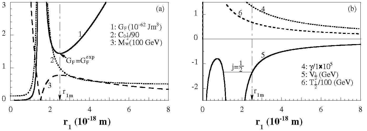
Figure 3: (a) $G_{\mbox{{\tiny{$F$}}}}=H_{I}r_{1}^{3}$, $C_{0{\mbox{\tiny{$\frac{1}{2}$}}}}$, $M_{\mbox{\tiny{w}}}$ (curves 1,2,3), and (b) $\gamma{}$, $V_{\mbox{\tiny{$\frac{1}{2}$}}}=-H_{I}$, $T_{\mbox{\tiny{$\frac{1}{2}$}}}$ (curves 4,5,6) as functions of $r_{1}$ computed from Eqs (F), (Dc), (E), (Fa), (D), (Da) for $\bar{\hskip 2.84544pta}=1.5391(8)\times 10^{-18}$ m. At $r_{1}=r_{1m}=2.5369(5)\times 10^{-18}$ m, $G_{\mbox{{\tiny{$F$}}}}=G_{\mbox{{\tiny{$F$}}}}^{exp}=1.43585(37)\times 10^{-62}$ Jm³.

Characteristically, for a specified $\bar{\hskip 2.84544pta}$ value, the $G_{{\mbox{{\tiny{$F$}}}}}(r_{1})$ vs $r_{1}$ function presents an extremal point at a (uniquely specified) $r_{1}$, $r_{1m}$, at which $G_{{\mbox{{\tiny{$F$}}}}}(r_{1m})$ is a minimum satisfying Eq (F), as in Fig 3a, although this is not generally equal to $G_{\mbox{{\tiny{$F$}}}}^{exp}$. $G_{{\mbox{{\tiny{$F$}}}}}(r_{1m})$ increases monotonically with $\bar{\hskip 2.84544pta}$. Computing $G_{{\mbox{{\tiny{$F$}}}}}(r_{1m})$ as a function of $\bar{\hskip 2.84544pta}$ over a range of $\bar{\hskip 2.84544pta}$ values, a unique $\bar{\hskip 2.84544pta}$ is found at $\bar{\hskip 2.84544pta}=1.5391(8)\times 10^{-18}$ m at which $G_{\mbox{{\tiny{$F$}}}}(r_{1m})=G_{\mbox{{\tiny{$F$}}}}^{exp}$ satisfying Eq (F), $r_{1m}=2.5369(5)\times 10^{-18}$ m, $\gamma{}=1.3190\times 10^{5}$ (Eq Fa), and $C_{0{\mbox{\tiny{$\frac{1}{2}$}}}}=\left(\frac{4\pi}{3}\right)\times 3(1+1.3952+4.6633)=88.69$ (Eqs Eb, Dc). Note that the $\bar{\hskip 2.84544pta}$ value obtained is in accordance with the order of magnitude of the neutron charge radius, $\sim 1.4\times 10^{-18}$ m, measured by electron-neutron scattering experiment (see also Sec B.3).

With the $\bar{\hskip 2.84544pta}$, $r_{1m}$ (hence $C_{0{\mbox{\tiny{$\frac{1}{2}$}}}}$), $\upsilon_{\mbox{\tiny{$\frac{1}{2}$}}},\gamma{}$ values obtained, all the remaining dynamical variables and functions may be evaluated. For the fixed $\bar{\hskip 2.84544pta}=1.5392\times 10^{-18}$ m value, the $G_{\mbox{{\tiny{$F$}}}}$, $C_{0{\mbox{\tiny{$\frac{1}{2}$}}}}$, $M_{\mbox{\tiny{w}}}$ (using the average experimental value $\sin^{2}\theta_{\mbox{\tiny{w}}}=0.23$), $\gamma{}$, $V_{\mbox{\tiny{$\frac{1}{2}$}}}(=-H_{\mbox{\tiny{$\frac{1}{2}$}}})$, and $T_{{\mbox{\tiny{$\frac{1}{2}$}}}}$ vs. $r_{1}$ functions, computed from Eqs (F), (Eb,Dc), (Ea), (Fa), (D), (Da) are as shown in Figs 3a,b (curves 1–6). $r_{1}=r_{1.{\mbox{\tiny{min}}}}$ lies as expected in the region where $-\partial V_{\mbox{\tiny{$\frac{1}{2}$}}}(r)/\partial r=F_{\mbox{\tiny{$\frac{1}{2}$}}}(r)<0$, and $V_{\mbox{\tiny{$\frac{1}{2}$}}}(r)<0$. At $r_{1}=r_{1m}$, $V_{\mbox{\tiny{$\frac{1}{2}$}}}=-H_{I}=-1.310$ GeV, $T_{\mbox{\tiny{$\frac{1}{2}$}}}(\simeq{\mbox{$\mathscr{M}$}}c^{2})=67.36$ GeV, $H_{\mbox{\tiny{$\frac{1}{2}$}}}(\simeq E_{tot.{\mbox{\tiny{$\frac{1}{2}$}}}})=66.05$ GeV, $M_{\mbox{\tiny{w}}}=77.23$ GeV. Furthermore specifically, with the $\gamma{}$ value in (Fb),(Ba),(b), we obtain $\gamma{}_{\mbox{{\tiny{M}}}}=292.48(3)$, $\gamma{}_{e}=\gamma{}_{\mbox{{\tiny{M}}}}\frac{(M^{\mbox{\tiny{$0$}}}+K)}{2m_{e}^{\mbox{\tiny{$0$}}}}=3.0537(6)\times 10^{5}$, and $\gamma{}_{p}=\gamma{}_{\mbox{{\tiny{M}}}}\frac{(M^{\mbox{\tiny{$0$}}}-K)}{2m_{p}^{\mbox{\tiny{$0$}}}}=126.33$, which are $>>1$ each. So the particles $e,p$ within the neutron are travelling at velocities $\upsilon_{e}^{\prime},\upsilon_{p}^{\prime}\simeq c$ measured in their local space and time coordinates ${\bf r}_{e},t_{e},{\bf r}_{p},t_{p}$ (Eqs B) in the (non-inertial) CM frame; and so is the total mass $M$ at the CM relative to $e,p$. The total kinetic energy of $e,p$ in these absolute terms is given by substituting the $\upsilon_{e}^{\prime},\upsilon_{p}^{\prime},m_{e}(=km_{p}),m_{p}$ values in (B.2) as $T_{e}^{\prime}+T_{p}^{\prime}\dot{=}(k+1)m_{p}c^{2}=2.3165\gamma{}_{p}m_{p}^{\mbox{\tiny{$0$}}}c^{2}=2.3165\times 118.53=2\times 137.29$ GeV. Substituting $m_{e}=km_{p}$ into Eqs (Ba,b) gives the $e,p$ velocities measured in time $t$, $\upsilon_{e}=\frac{m_{p}}{M}\upsilon=\frac{c}{k+1}=0.43c$, $\upsilon_{p}=-\frac{m_{e}}{M}\upsilon=-\frac{kc}{k+1}=-0.57c$; and in turn the above values into Eq (B.2) gives the corresponding total kinetic energy $T_{e}+T_{p}=km_{p}(\frac{c}{k+1})^{2}+m_{p}(\frac{kc}{k+1})^{2}=\frac{k}{k+1}m_{p}c^{2}=0.56831\times 118.53=67.36$ GeV, equal to the solution value for $T_{{\mbox{\tiny{$\frac{1}{2}$}}}}={\mbox{$\mathscr{M}$}}c^{2}$ earlier. The non-inertial frame motion contributes an amount $(T_{e}^{\prime}+T_{p}^{\prime})-(T_{e}+T_{p})=(k+1)m_{p}c^{2}-\frac{k}{k+1}m_{p}c^{2}=\frac{k^{2}+k+1}{k+1}m_{p}c^{2}=1.75m_{p}c^{2}$. The exceedingly large kinetic energy apparently is mainly consumed to contract the size of the system.

The author expresses thanks to emeritus scientist P-I Johansson for his private financial support of the author’s research, to Kissemiss Johansson for his joyful companion when the unification researches were carried out, and to Professor C Burdik for providing the opportunity of presenting this wok at the 23rd International Conference on Integrable Systems and Quantum Symmetries (ISQS23), Tech Univ, Prague, June 2015, during which the author also very much enjoyed interesting discussions with a number of participants.

Appendix G Mapping of the spin current loop on to reduced geometries

Consider here the circular spin current loop of proton as projected in the $x_{p}^{s}y_{p}^{s}$ plane, spinning at tangential velocity $\upsilon^{s}_{p_{xy}}$ about the $z_{p}^{s}$ axis passing through ${\bf r}_{p}$ in counterclockwise sense, i.e. in spin up state as in Sec C.1. $dq_{p}=\rho_{pxy}a_{p}d\phi_{p}^{s}$ is a charge element at $\boldsymbol{\xi}_{p}(\phi^{s}_{p})$ on it. The magnetic field produced by this spin current loop at a distance ${\bf r}$ from ${\bf r}_{p}$ has the general form (Biot-Savart law) ${\bf B}_{p}^{s}({\bf r})=\int d{\bf B}_{p\theta}^{s}({\bf r}^{\prime})=\int\frac{dq_{p}{\boldsymbol{\upsilon}}^{s}_{p_{xy}}\times{\bf r}^{\prime}}{4\pi\epsilon_{0}c^{2}r^{\prime}{}^{3}}$, where ${\bf r}^{\prime}={\bf r}+\boldsymbol{\xi}_{p}(\phi_{p}^{s})$. The integration in algebraic terms is a complex problem. We below reduce the current loop to simpler geometries to facilitate an effective algebraic expression for the field (Eq D, Sec D).

Consider first this field produced at a point at distance $x_{p}^{s}=|{\bf r}|$ from ${\bf r}_{p}$ on the positive $x_{p}^{s}$ axis, ${\bf B}_{p}^{s}(x_{p}^{s}=|{\bf r}|)$; $x_{p}^{s}$ is on the right side to the $z_{p}^{s}$ axis as plotted for the parallel $x,y,z$ axes of $x_{p}^{s},y_{p}^{s},z_{p}^{s}$ in Fig 1b. The problem has the obvious symmetry that the left-half current loop produces at $x_{p}^{s}$ a magnetic field ${\bf B}_{p{\mbox{\tiny{$L$}}}}^{s}(\propto{\boldsymbol{\upsilon}}_{pxy}^{s}\times{\bf x}_{p}^{s})>0$ in $+z$ direction, and the right-half a field ${\bf B}_{p{\mbox{\tiny{$R$}}}}^{s}<0$ in $-z$ direction. The total field ${\bf B}_{p{\mbox{\tiny{$R$}}}}^{s}-{\bf B}_{p{\mbox{\tiny{$L$}}}}^{s}={\bf B}_{p}^{s}(x_{p}^{s}=|{\bf r}|)$ is in $-z$ direction. Furthermore, on either half loop the differential $d{\bf B}_{p}^{s}$ fields produced by all charge elements as associated with the $y$-component velocities add up, and with the $x$-component velocities cancel out. So, in so far as the same ${\bf B}_{p{\mbox{\tiny{$L$}}}}^{s},{\bf B}_{p{\mbox{\tiny{$R$}}}}^{s}$ are in effect produced, the left- and right- half spin current loops may be further reduced to two point half-charges $+\frac{1}{2}e,+\frac{1}{2}e$ located at effective distances $-\bar{\hskip 2.84544pta},\bar{\hskip 2.84544pta}$ from ${\bf r}_{p}$ on the $x_{p}^{s}$ axis and moving oppositely at velocities $-\bar{\bf{\upsilon}}_{pxy}^{s}{},\bar{\bf{\upsilon}}_{pxy}^{s}{}$ in the $-y_{p}^{s},+y_{p}^{s}$ directions, where

$$\halign{\hbox to\displaywidth{$\hfil\displaystyle#\hfil$}\cr 0.0pt{\hfil$\displaystyle\hfill\bar{\hskip 2.84544pta}=\eta a,\quad\bar{\upsilon}_{pxy}^{s}=\bar{\upsilon}_{p}^{s}\cos\theta_{p}^{s},\quad\bar{\upsilon}_{p}^{s}=\bar{\hskip 2.84544pta}\omega{}_{p}^{s}=\eta a\omega{}_{p}^{s}=\eta\upsilon_{p}^{s},\quad\upsilon_{p}^{s}=a\omega{}_{p}^{s};\hfill(\ref{eq-app-aav})\crcr}}$$

$\eta$ is a coefficient to be determined. We have set $a=a_{p}=a_{e}=\frac{1}{2}(a_{e}+a_{p})$ here; so $\bar{\hskip 2.84544pta}$ is effective also in its being scaled by $\eta$ from the average radius $a$ of the $e,p$ charges. In analogy to $r=r^{\mbox{\tiny{$0$}}}/\gamma{}$, $a$ is contracted from its rest value $a^{\mbox{\tiny{$0$}}}$ formally according to $a=a^{\mbox{\tiny{$0$}}}/\gamma{}_{a}$; $\gamma{}_{a}$ is a factor analogous to $\gamma{}$, being an increasing function with $(\upsilon_{p}/c)^{2}$.

By virtue of its physical significance, $\bar{\hskip 2.84544pta}$ should be such that the moments of inertia of the right and left point half-charges about the $z_{p}^{s}$ axis, $I_{{\mbox{\tiny{$R$}}}}^{point}$, $I_{{\mbox{\tiny{$L$}}}}^{point}(=I_{{\mbox{\tiny{$R$}}}}^{point})$, are equal to those of the half current loops about $z_{p}^{s}$, $I_{{\mbox{\tiny{$R$}}}}^{loop}$, $I_{{\mbox{\tiny{$L$}}}}^{loop}(=I_{{\mbox{\tiny{$R$}}}}^{loop})$. Let $m_{p}^{*}$ be the effective mass uniformly distributed along the full current and in turn on the full charge, and hence a mass $\frac{1}{2}m_{p}^{*}$ on each half loop and in turn at each half point charge. The moments of inertia of one point half charge and one half loop are known as, written for the right ones,

$$\halign{\hbox to\displaywidth{$\hfil\displaystyle#\hfil$}\cr 0.0pt{\hfil$\displaystyle\hfill I_{{\mbox{\tiny{$R$}}}}^{point}=\frac{1}{2}m_{p}^{*}\bar{\hskip 2.84544pta}^{2},\quad I_{{\mbox{\tiny{$R$}}}}^{loop}=\int^{\pi}_{0}x^{2}dm_{p}^{*}=2\int^{\pi/2}_{0}(a_{p}\cos\phi)^{2}\frac{(m_{p}^{*}/2)}{\pi}d\phi=\frac{m_{p}^{*}a^{2}}{4}\hfill(\ref{eq-app-Is})\crcr}}$$

The equality $I_{{\mbox{\tiny{$R$}}}}^{loop}=I_{{\mbox{\tiny{$R$}}}}^{{\rm{point}}}$ gives $\frac{1}{2}\bar{\hskip 2.84544pta}^{2}(=\frac{1}{2}(\eta a)^{2})=\frac{1}{4}a^{2}$, so $\eta=1/\sqrt{2}$. Accordingly, the right point half-charge is associated with a spin angular momentum $S_{p{\mbox{\tiny{$R$}}}}=I_{{\mbox{\tiny{$R$}}}}^{{\rm{point}}}\omega{}_{p}^{s}(=I_{{\mbox{\tiny{$R$}}}}^{loop}\omega{}_{p}^{s})=\frac{1}{2}m_{p}^{*}\bar{\hskip 2.84544pta}^{2}\omega{}_{p}^{s}=\frac{1}{2}m_{p}^{*}\bar{\hskip 2.84544pta}\bar{\upsilon}_{p}^{s}$, so that the $z$ component is $S_{p{\mbox{\tiny{$R$}}}z}=S_{p{\mbox{\tiny{$R$}}}}\cos\theta_{p}^{s}=\frac{1}{2}m_{p}^{*}\bar{\hskip 2.84544pta}\bar{\upsilon}_{p_{xy}}^{s}$.

Now with respect to a point at a distance ${\bf x}_{p}^{s}{}^{\prime\prime}$ from ${\bf r}_{p}$ on the $x^{\prime\prime}$ axis (Sec B.4) lying in a plane whose normal is along the $z^{\prime}$ or $z^{\prime\prime}$ direction at angle $\theta_{j}$ to the $z$ axis, with $|{\bf x}_{p}^{s}{}^{\prime\prime}|=|{\bf x}_{p}^{s}|=|{\bf r}|$, the component spin angular momentum of the right point half-charge perpendicular to $x^{\prime\prime}$ is the projection of $S_{p{\mbox{\tiny{$R$}}}z}$ onto the $z^{\prime\prime}$ or $z^{\prime}$ direction,

$$\halign{\hbox to\displaywidth{$\hfil\displaystyle#\hfil$}\cr 0.0pt{\hfil$\displaystyle\hfill S_{p{\mbox{\tiny{$R$}}}z}^{\prime\prime}=S_{p{\mbox{\tiny{$R$}}}z}\cos\theta_{j}=\frac{1}{2}m_{p}^{*}\bar{\hskip 2.84544pta}\bar{\upsilon}_{p_{xy}}^{s}\cos\theta_{j}=\frac{1}{2}m_{p}^{*}\bar{\hskip 2.84544pta}\bar{\upsilon}_{p}^{s}{}^{\prime\prime},\quad\bar{\upsilon}_{p}^{s}{}^{\prime\prime}=\bar{\upsilon}_{p_{xy}}^{s}\cos\theta_{j}=\bar{\upsilon}_{p}^{s}\cos\theta_{p}^{s}\cos\theta_{j}\hfill(\ref{eq-app-SpzRp})\crcr}}$$

Appendix H Stable-state solution for $r_{\mbox{\tiny{$l$}}}$

Substituting $\frac{d^{2}{\bf r}_{{\mbox{\tiny{$l$}}}{\mbox{\tiny{$j$}}}}}{dt^{2}}=-\frac{\upsilon_{\mbox{\tiny{$j$}}}^{2}}{r_{\mbox{\tiny{$l$}}}}\hat{r}_{{\mbox{\tiny{$l$}}}{\mbox{\tiny{$j$}}}}$, $\upsilon_{j}$ from (B.1)^′, and ${\bf{F}}_{{\mbox{\tiny{$j$}}}}$ from (D) into (Bd) gives $-{\mbox{$\mathscr{M}$}}\frac{(4l^{2}-1)\hbar^{2}\,\hat{r}}{4{\mbox{$\mathscr{M}$}}^{2}r_{\mbox{\tiny{$l$}}}^{3}}=-\frac{f_{t}^{2}e^{2}\hbar^{2}\hskip 0.56917ptC^{{\atop-}\hskip 2.27626pt}{}_{0j}\,\hat{r}}{16\pi\epsilon_{0}m_{e}m_{p}c^{2}r_{\mbox{\tiny{$l$}}}^{4}}$. Cancelling common factors on both sides, sorting, with $f_{t}^{2}=4$ for $m_{e}=1.3165m_{p}$ (Sec D) and $M=\gamma{}_{{\mbox{{\tiny{M}}}}}^{(j)}M^{\mbox{\tiny{$0$}}}$ for $j$th state, we obtain

$$\halign{\hbox to\displaywidth{$\hfil\displaystyle#\hfil$}\cr 0.0pt{\hfil$\displaystyle\hfill r_{\mbox{\tiny{$l$}}}=\frac{e^{2}\hskip 0.56917ptC^{{\atop-}\hskip 2.27626pt}{}_{0j}}{(4l^{2}-1)\pi\epsilon_{0}\gamma{}_{\mbox{{\tiny{M}}}}^{(j)}M^{\mbox{\tiny{$0$}}}c^{2}}.\quad{\rm For}\ j=\frac{1}{2},\ l=1:\ \ r_{1}=\frac{e^{2}\hskip 0.56917ptC^{{\atop-}\hskip 2.27626pt}{}_{0{\mbox{\tiny{$\frac{1}{2}$}}}}}{3\pi\epsilon_{0}\gamma{}_{\mbox{{\tiny{M}}}}^{({\mbox{\tiny{$\frac{1}{2}$}}})}M^{\mbox{\tiny{$0$}}}c^{2}};\hfill(\ref{eq-r1stab})\crcr}}$$

for $j=\frac{3}{2}$, $l=2$, $r_{2}=\frac{e^{2}\hskip 0.56917ptC^{{\atop-}\hskip 2.27626pt}{}_{0\frac{3}{2}}}{15\pi\epsilon_{0}\gamma{}_{\mbox{{\tiny{M}}}}^{(3/2)}{M^{\mbox{\tiny{$0$}}}}c^{2}}$, $\hskip 0.56917ptC^{{\atop-}\hskip 2.27626pt}{}_{0\frac{3}{2}}=15+\frac{3\sqrt{g_{e}g_{p}}}{2C_{12}}+\frac{9g_{e}g_{p}}{10C_{12}}$ given after Eq (Db). For the $j=\frac{1}{2}$ state, with (Db) for $\hskip 0.56917ptC^{{\atop-}\hskip 2.27626pt}{}_{0{\mbox{\tiny{$\frac{1}{2}$}}}}$, (Dc) for $C_{11}$, and $\bar{\hskip 2.84544pta}=1.53918\times 10^{-18}$ m, the right side of (Hb) may be computed as a function of $r_{1}$. Two numerical solutions are found at $r_{1}=1.440\times 10^{-18}$, $1.661(7)\times 10^{-18}$ m, at which the two sides of (Hb) are equal.

Part C (Published in J. Phys.: Conf. Ser. 1416 012043, 2019)

Appendix A Introduction

In the Standard Model (SM) description[1, 2], elementary particles are divided into $2\times 6$ leptons, baryons / mesons made of $2\times 6$ quarks, and five or so force mediators. Regarding their weak decays, such as the neutron $\beta$ decay $n\rightarrow e^{\mbox{-}}p{\bar{\nu}}_{e}$, the SM quark model assumes that the decay product particles $e^{\mbox{-}},p,{\bar{\nu}}_{e}$ do not exist until $n$ decays, and that they are instantaneously produced and emitted upon the $n$ decay. The SM has been successful in reproducing the charges, spins, C, P and T symmetries of the hundreds of observational elementary particles, and predicting their decay rates -absolute or comparative. But the SM has unnatural aspects, concerning the quarks and weak decays in particular. The baryons and mesons are made of quarks rather than the particles they decay into, which is an abrupt departure from the atomic and nuclear descriptions. Free quarks are never observed in experiment. The SM weak interaction Hamiltonian $H=G/(\frac{4\pi}{3}r^{3})$ is a phenomenological construction. The weak force is not predicted. The weak, strong, gravitational and electromagnetic forces are not unified. The basic questions common to the regular particles $e^{\mbox{-}},p$ (being the two only permanent particles - why?) remain outstanding, including the origin of mass, the nature of matter waves, and the cause of gravity.

The Internally Electrodynamic (IED) particle model (see a review and the original references given in [4]) is a complementary approach to the SM and is beyond the SM. The IED model was developed using overall observational properties of particles as input information, and aimed from the beginning to achieve a unification of the three basic mechanics and of the four fundamental forces. In terms of this model, the electron $e^{\mbox{-}}$ and the proton $p$ are composed of oscillatory charges $-e$ and $+e$ and their electromagnetic radiation (EMR) fields in a polarisable dielectric vacuum filled of vacuuons[7, 8]. Their distinct masses are uniquely determined [9] by the quantum oscillation levels of $-e,+e$ in their vacuum potentials that are asymmetric to $-e,+e$. The masses of their antiparticles $e^{\mbox{-}},\bar{p}$ are determined because of pair productions. The remaining single charged particles, including the six manifestly free forms $\pi^{\mp}$, $\mu^{\mp}$, $\tau^{\mp}$ and ones in (confined) higher excited states such as comprising $\rho^{0}(770)$, are the main subject of investigation of this paper. We shall show that, in accordance to the overall experimental demonstrations, these can be generally each described as a charge $-e$ or $+e$ oscillation and the resulting EMR originally generated in the weak potential field of another particle, that are as a whole in certain precessional orbital (P-O) motions. The remaining unstable elementary matter particles such as $n$, ${{\mit\Lambda}}$, $\pi^{0}$, $\rho(770)$ are composites of two or more of the single charged ones. A formal $e^{\mbox{-}},p$ model of the neutron $n$ and first principles solutions for spin, magnetic -hence weak- interaction force, coupling constant, and (unpublished) mixing angle have been achieved in [5]. The ${{\mit\Lambda}}$-hyperon is the simplest baryon emitting a pion ${\pi^{\mbox{-}}}$, but otherwise a direct analogue of $n$, and will serve a prototype system for the model constructions in this paper.

The formal representation divides in three sections. In Sec B, using the relevant observations as input information we propose the existence of mass states ”heavy electrons (or positrons)”, originally generated by charges $-e$’s (or $+e$’s) in the weak potential fields of other particles. In terms of this we propose the structures of the pions $\pi^{\mp}$ and muon $\mu^{\mp}$. In Sec C, we present a generalised first principles description of the masses of the single charged particles such as $\pi^{\mp},\mu^{\mp}$, $e^{\mbox{-}}$, $p$, and the composite particles such as $n,{{\mit\Lambda}}$. In Sec D, we predict the existence of a double heavy positronium preceding the rudimentary productions of $\mu^{\mp},\pi^{\mp}$, etc. and, based on its eigen level $n=2$ solutions, we ab initio predict the masses of $\mu^{\mp}$, $\pi^{\mp}$. Representation of the remaining composite unstable elementary particles will be described in a separate paper.

Appendix B Structures of the charged pions and muons

B.1 The charged pions $\pi^{\mbox{-}},{\pi^{\mbox{\footnotesize{$+$}}}}$   The simplest composite baryon emitting a charged pion $\pi^{\mbox{-}}$, and secondarily a muon $\mu^{\mbox{-}}$, is the ${{\mit\Lambda}}$ hyperon. Observationally, ${{\mit\Lambda}}$ has an identical charge $0$, spin $\frac{1}{2}$, and analogous decay reaction ${{\mit\Lambda}}\rightarrow\pi^{\mbox{-}}p\rightarrow\mu^{\mbox{-}}{\bar{\nu}}_{\mu}p$ to those of the neutron $n$ ($n\rightarrow e^{\mbox{-}}{\bar{\nu}}_{e}p$), but has a heavier mass 1115.6 MeV. These suggest an analogous structure of ${{\mit\Lambda}}$ to $n$ [5] (Fig Ba, Inset), except in place of ${e^{\mbox{-}}}$ of $n$, ${{\mit\Lambda}}$ has a ”heavy electron” ($h^{\mbox{-}}$) in P-O motion relative to $p$ (Fig Ba). In accordance to the implication of ${{\mit\Lambda}}$, the observational $\pi^{\mbox{-}}$ charge $-e$, spin $s_{\pi}=0$, mass $M_{\pi}=139.569$ MeV, decay reaction $\pi^{\mbox{-}}\rightarrow\mu^{\mbox{-}}{\bar{\nu}}_{\mu}\rightarrow(e^{\mbox{-}}{\bar{\nu}}_{e}\nu_{\mu}){\bar{\nu}}_{\mu}$ and rudimentary direct production reaction $e^{\mbox{-}}e^{\mbox{\footnotesize{$+$}}}\rightarrow\rho(770)\rightarrow\pi^{\mbox{-}}\pi^{\mbox{\footnotesize{$+$}}}$, we propose a two-step description of the $\pi^{\mbox{-}}$ structure: (1) There presents a (confined) particle state called heavy electron, $h^{\mbox{-}}$, that has a charge $-e$, spin $\frac{1}{2}$ as the electron $e^{\mbox{-}}$, and yet is a heavier mass state, the charge $-e$ oscillation and its resultant EMR of a mass $M_{h}$, (originally) generated in the weak potential field $V_{\mbox{\tiny{$\frac{1}{2}$}}}$ of another particle. (2) The pion $\pi^{\mbox{-}}$ is a heavy electron $h^{\mbox{-}}$, of spin $S_{hz}=\frac{1}{2}\hbar$ in $z$ direction, in P-O (precessional-orbital) motion at essentially the light speed, $\upsilon_{\mbox{\tiny{$\frac{1}{2}$}}}\dot{=}c$, along ${\bar{\nu}}_{e}$-orbit of a normal ($-z^{\prime}$) at quantised angle $\pi-\theta_{\mbox{\tiny{$\frac{1}{2}$}}}$ to the $z$ axis (Fig Bb), in the absence of other particle(s). The P-O kinetic energy current along ${\bar{\nu}}_{e}$ resembles a confined antineutrino ${\bar{\nu}}_{e}$, of an apparent rest mass $M_{\nu_{e}}$. Two equal but opposite P-O momentum currents along ${\bar{\nu}}_{\mu}$ $\nu_{\mu}$ (hence confined neutrinos) are generated momentarily upon $\pi^{\mbox{-}}$ decay in an explosive collision (Fig Bb, Inset), these do not contribute to the ${\pi^{\mbox{-}}}$ dynamical variables. By virtual of its anti-symmetric properties, $\pi^{\mbox{\footnotesize{$+$}}}$ is a heavy positron $h^{\mbox{\footnotesize{$+$}}}$ in P-O motion along orbit $\nu_{e}$. The rest mass of $\pi^{\mbox{-}}$ (or $\pi^{\mbox{\footnotesize{$+$}}}$) is formally $M_{\pi}=M_{h}+M_{{\bar{\nu}}_{e}}$.

The $z$ component and the total angular momenta of the P-O motion of $h^{\mbox{-}}$ are given by the eigen solutions of bound state $n=2$, ${\mbox{\footnotesize{$l$}}}=1$, $j={\mbox{\footnotesize{$l$}}}-{\mbox{\footnotesize{$l$}}}^{\mbox{{\tiny{$TP$}}}}=\frac{1}{2}$ in the original $V_{\mbox{\tiny{$\frac{1}{2}$}}}$ field (e.g. of $p$ as in ${{\mit\Lambda}}$) in the lab frame similarly as for $n$ ([5]), $J_{{\mbox{\tiny{$\frac{1}{2}$}}}z}=J_{{\mbox{\tiny{$\frac{1}{2}$}}}}\cos(\pi-\theta_{\mbox{\tiny{$\frac{1}{2}$}}})=-j\hbar=-\frac{1}{2}\hbar$, $J_{{\mbox{\tiny{$\frac{1}{2}$}}}}=|{\bf r}_{{\mbox{\tiny{$\frac{1}{2}$}}}\pi}\times(m_{\pi}{\boldsymbol{\upsilon}}_{{\mbox{\tiny{$\frac{1}{2}$}}}})|(=|{\bf r}_{{\mbox{\tiny{$\frac{1}{2}$}}}{\mbox{\tiny{${{\mit\Lambda}}$}}}}\times({\mathscr{M}}_{\mbox{\tiny{${{\mit\Lambda}}$}}}{\boldsymbol{\upsilon}}_{{\mbox{\tiny{$\frac{1}{2}$}}}{\mbox{\tiny{${{\mit\Lambda}}$}}}})|)=\sqrt{j(j+1)}|_{j=1/2}\hbar=\frac{\sqrt{3}}{2}\hbar$, where $\cos(\pi-\theta_{\mbox{\tiny{$\frac{1}{2}$}}})=-\frac{1}{\sqrt{3}}$, $m_{\pi}=\gamma{}_{\pi}M_{\pi}$, $\gamma{}_{\pi}=(1-(\upsilon_{\mbox{\tiny{$\frac{1}{2}$}}}/c)^{2})^{-1/2}$ (${\mathscr{M}}_{\mbox{\tiny{${{\mit\Lambda}}$}}}$, is the reduced mass and $r_{1{\mbox{\tiny{${{\mit\Lambda}}$}}}}$ the orbit radius of $\pi^{\mbox{-}},p$ comprising ${{\mit\Lambda}}$). Those of the total system $\pi^{\mbox{-}}(e_{h}^{\mbox{-}}[{\bar{\nu}}_{e}])$ are $S_{\pi z}=J_{{\mbox{\tiny{$\frac{1}{2}$}}}z}+S_{hz}=(-\frac{1}{2}+\frac{1}{2})\hbar=s_{\pi}\hbar=0$, $s_{\pi}=0$, and $S_{\pi}=\sqrt{s_{\pi}(s_{\pi}+1)}\hbar=0$. The kinetic energy is $T_{\pi}=\frac{\gamma{}}{\gamma{}+1}m_{\pi}\upsilon_{\mbox{\tiny{$\frac{1}{2}$}}}^{2}=\frac{\gamma{}}{\gamma{}+1}J_{\mbox{\tiny{$\frac{1}{2}$}}}c/r_{1}$.

B.2 The muons $\mu^{\mbox{-}},{\mu^{\mbox{\footnotesize{$+$}}}}$   In direct accordance to the observational charge $-e$, spin $s_{\mu}=\frac{1}{2}$, mass $M_{\mu}=105.658$ MeV and decay reaction $\mu^{\mbox{-}}\rightarrow e^{\mbox{-}}{\bar{\nu}}_{e}\nu_{\mu}$ of $\mu^{\mbox{-}}$, to its specific production from $\pi^{\mbox{-}}\rightarrow\mu^{\mbox{-}}{\bar{\nu}}_{\mu}$ and the $\pi^{\mbox{-}}$ structure of Sec B.1, we propose: By an apparent loss of mass energy of its motion in the $y^{\prime}z$ plane(s), $h^{\mbox{-}}$ transforms to a $xy$-projected mass state ${h^{\mbox{-}}_{xy}}$ of mass $M_{{{h}_{xy}}}$, and of an unchanged charge $-e$ and spin $s_{h_{{xy}}}=\frac{1}{2}=S_{h_{{xy}}z}/\hbar$ in $+z$ direction here. The muon $\mu^{\mbox{-}}$ is a ${h^{\mbox{-}}_{xy}}$ in rotational motion along two coinciding elliptics $\nu_{y^{\prime}z}$, $\nu_{y^{\prime\prime}z}$ projected from the ${\bar{\nu}}_{e}$-, $\nu_{\mu}$-orbits in a $y^{\prime}z$ (or $y^{\prime\prime}z$) plane. $\nu_{y^{\prime}z}$ is the result of supposition of two P-O motions, at speed $\upsilon_{\mbox{\tiny{$\frac{1}{2}$}}}\dot{=}c$ each, along ${\bar{\nu}}_{e}$-, $\nu_{\mu}$-orbits of equal radius $r_{1\mu}$, and of normals $z^{\prime},z^{\prime\prime}$ at quantised angles $\pi-\theta_{\mbox{\tiny{$\frac{1}{2}$}}}$ and $\theta_{\mbox{\tiny{$\frac{1}{2}$}}}$ to the $z$ axis (Fig Ba).

The projections of the ${\bar{\nu}}_{e}$-,$\nu_{\mu}$- orbits in the $y^{\prime}z$ plane, $\nu_{y^{\prime}z}$,$\nu_{y^{\prime\prime}z}$, or in the $xy$ plane, $\nu_{xy}$’s, necessarily coincide. The component kinetic motions of $-e$ along $\nu_{xy}$’s are thus equal and opposite and cancel out, leaving ${h^{\mbox{-}}_{xy}}$ at rest on $\nu_{xy}$ at a random angle $\varphi$ to the $x$ axis, and those along $\nu_{y^{\prime}z}$,$\nu_{y^{\prime\prime}z}$ add up. Similarly as for $n$[5] and $\pi^{\mbox{-}}$ (Sec B.1), the angular momenta of the P-O motions along ${\bar{\nu}}_{e},\nu_{\mu}$ are each given by the eigen solutions in the states $n=2$, ${\mbox{\footnotesize{$l$}}}=1$, $j={\mbox{\footnotesize{$l$}}}-{\mbox{\footnotesize{$l$}}}^{\mbox{{\tiny{$TP$}}}}=\frac{1}{2}$ in the lab frame: $J_{{\mbox{\tiny{$\frac{1}{2}$}}}}=r_{1\mu}\gamma{}_{\mu}M_{\mu}c=\sqrt{j(j+1)}\hbar=\frac{\sqrt{3}}{2}\hbar$. The projections along $z$ (with $m_{j}^{\prime},m_{j}^{\prime\prime}=-\frac{1}{2},\frac{1}{2}$) are $J_{{\mbox{\tiny{$\frac{1}{2}$}}}z}^{\prime}=-J_{{\mbox{\tiny{$\frac{1}{2}$}}}z}^{\prime\prime}=J_{\mbox{\tiny{$\frac{1}{2}$}}}\cos(\pi-\theta_{\mbox{\tiny{$\frac{1}{2}$}}})=-\frac{1}{2}\hbar$, and in the $xy$ plane are $J_{{\mbox{\tiny{$\frac{1}{2}$}}}xy}^{\prime}=J_{{\mbox{\tiny{$\frac{1}{2}$}}}xy}^{\prime\prime}=J_{\mbox{\tiny{$\frac{1}{2}$}}}\sin\theta_{\mbox{\tiny{$\frac{1}{2}$}}}=\frac{\sqrt{2}}{2}\hbar$, where $\cos\theta_{\mbox{\tiny{$\frac{1}{2}$}}}=1/\sqrt{3}$, $\sin\theta_{\mbox{\tiny{$\frac{1}{2}$}}}=\sqrt{2/3}$. $J_{{\mbox{\tiny{$\frac{1}{2}$}}}xy,\mu}=J_{{\mbox{\tiny{$\frac{1}{2}$}}}xy}^{\prime}+J_{{\mbox{\tiny{$\frac{1}{2}$}}}xy}^{\prime\prime}=\sqrt{2}\hbar$ at angle $\varphi$ to $x$ in the $xy$ plane, of a time average $\langle J_{{\mbox{\tiny{$\frac{1}{2}$}}}xy,\mu}\rangle=0$. The spin (angular momentum) of the total system $\mu^{\mbox{-}}(h^{\mbox{-}}_{{xy}}[{\bar{\nu}}_{e},\nu_{\mu}])$ is $S_{\mu z}=S_{{{h}_{xy}},z}+J_{{\mbox{\tiny{$\frac{1}{2}$}}}z,\mu}=\frac{1}{2}\hbar$ in $+z$ direction.

Figure B. Schematic structures of (a) ${{\mit\Lambda}}$ in analogy to $n$ (Inset.a), except in place of $e^{\mbox{-}}$, in ${{\mit\Lambda}}$ is a heavy electron $h^{\mbox{-}}$ in P-O motion shown in the $p$ rest frame, and (b) stationary $\pi^{\mbox{-}}$; (Inset.b) shows ${\pi^{\mbox{-}}}$ just before decay.

Figure B. (a) Schematic structure of $\mu^{\mbox{-}}$, which is a ${h^{\mbox{-}}_{xy}}$ of charge $-e$, spin $\frac{1}{2}$, and in two superposing P-O motions along orbits $\nu_{\mu},{\bar{\nu}}_{e}$ of normals $z^{\prime},z^{\prime\prime}$ at angles $\pi-\theta_{1/2}$, $\theta_{1/2}$ to the $z$ axis. (b) $e^{\mbox{-}},e^{\mbox{\footnotesize{$+$}}}$ near head-on collision at separation $r^{*}_{2,1}$ to form a double heavy positronium, preceding to $\mu^{\mbox{-}}\mu^{\mbox{\footnotesize{$+$}}}$ production.

Appendix C A generalised IED model extending to weak potential field

In the IED picture, the mass of a single charged permanent particle $\alpha$ (e.g. ${e^{\mbox{-}}}$) is generated by the oscillation of its charge $q(=-e)$, of a displacement $u_{q}$ (of the CM of the minute but extensive $q$), in the vacuum potential field $V_{\rm v}$ (mainly due to $q$ and vacuuon-dipoles’ electrostatic interaction) [4, 9]. In absence of other particles, $V_{{\rm v}}=\widetilde{V}_{\rm v}+V_{{\rm v}0}\dot{=}\frac{1}{2}\beta_{{\rm v}}u_{q}^{2}+V_{{\rm v}0}$, where $\beta_{{\rm v}}={\mathfrak{M}}_{\rm v}{{\mit{\Omega}}}_{\rm v}^{2}$ is the force constant, ${\mathfrak{M}}_{\rm v}$ is the (sub-vacuum) mass of the charge $q$, and ${{\mit{\Omega}}}_{\rm v}$ is the angular frequency. Assume $q$ oscillates about a fixed position and hence $\alpha$ is at rest. ${\mathfrak{M}}_{\rm v}$ represents a friction against the $q$ motion ordinarily in its own $V_{{\rm v}}$ field. If another particle $\alpha^{\prime}$ of charge $q^{\prime}$ presents in the vicinity and exerting on the vacuum a potential $\widetilde{V}_{\rm v}^{\prime}$, then ${\mathfrak{M}}_{\rm v}$ ($\propto$ friction), hence $\beta_{\rm v}$, $\widetilde{V}_{\rm v}$ of $q$ of $\alpha$ would in general be modified, by a factor $\eta_{\rm v}$ to ${\mathfrak{M}}_{\rm v}^{\mbox{\tiny${\dagger}$}}$, $\beta_{\rm v}^{\mbox{\tiny${\dagger}$}}$, and

$$\halign{\hbox to\displaywidth{$\hfil\displaystyle#\hfil$}\cr 0.0pt{\hfil$\displaystyle\hfill\mbox{$\widetilde{V}_{\rm v}^{\mbox{\tiny${\dagger}$}}(u_{q})=\frac{1}{2}\beta_{\rm v}^{\mbox{\tiny${\dagger}$}}u_{q}^{2}=\frac{1}{2}\beta_{\rm v}u_{q}^{2}+\frac{1}{2}{\cal{O}}_{\eta}c^{2},\quad\beta_{\rm v}^{\mbox{\tiny${\dagger}$}}=\beta_{\rm v}(1+\frac{{\cal{O}}_{\eta}c^{2}}{2\langle\widetilde{V}_{{\rm v}}\rangle}),\quad{\cal{O}}_{\eta}=\frac{\eta_{\rm v}D\langle\widetilde{V}_{{\rm v}^{\prime}}\rangle}{D^{\prime}c^{2}},$}\hfill(\ref{eq-DV.Fp.b-p})\crcr}}$$

where $D,D^{\prime}$ are the dimensions of the $q,q^{\prime}$ oscillations; $\langle\ \rangle$ indicates the time average.

Consider a particle $\alpha$ of charge $q$ is in P-O motion along orbit ${\bar{\nu}}$ (of a normal $z^{\prime}$) relative to $\alpha^{\prime}$ in the central magnetic or weak potential field of $\alpha^{\prime}$ $V_{\mbox{\tiny{$\frac{1}{2}$}}}(r_{1})=-G/(\frac{4}{3}\pi r_{1}^{3})$, at an (equilibrium) separation $r_{1}(\sim 10^{-18}$ m), $G$ being the coupling constant. Attach the local co-ordinate axes $\xi,\zeta$ to the moving $\alpha$, with an origin fixed at $r_{1}$ and $\xi,\zeta$ parallel to $r$, $z^{\prime}$ (the radius and normal of orbit ${\bar{\nu}}$). The oscillation of (the CM of) $q$, of displacement ${\bf{u}}_{q}={\bf r}-{\bf r}_{1}=\boldsymbol{\xi}_{q}+\boldsymbol{\zeta}_{q}$, in $\widetilde{V}_{\rm v}$ is now in the (instantaneous) $\xi,\zeta$ plane of dimension $D=2$, at a random angle $\vartheta$ to $\zeta$, and of a rest amplitude ${\cal{A}}_{{\rm v}\vartheta}={\cal{A}}_{{\rm v}}|\sin\vartheta\hat{\xi}+\cos\vartheta\hat{\zeta}|=|{\cal{A}}_{{\rm v}\xi}\hat{\xi}+{\cal{A}}_{{\rm v}\zeta}\hat{\zeta}|$; $\vartheta$ varies randomly in $2\pi$ over time. Consider further $q$ is at initial time driven by an external force (${\bf{F}}_{ext}$) into displacement $\xi_{q}$ from $r_{1}$ along radial $r$- or $\xi$- direction. After a relaxation time $q$ maintains an oscillation of displacement $\xi_{q}(t)=r-r_{1}={\cal{A}}_{h}\psi_{q}(t)$, expressed for a free $\alpha$ at rest here, under the restoring force ${\bf{F}}_{h}=-\frac{\partial V_{h}}{\partial\xi_{q}}\hat{\xi}$ produced by one half of the difference weak potential,

$$\halign{\hbox to\displaywidth{$\hfil\displaystyle#\hfil$}\cr 0.0pt{\hfil$\displaystyle\hfill V_{h}(\xi_{q})=\frac{1}{2}[V_{{\mbox{\tiny{$\frac{1}{2}$}}}}(r_{1}+\xi_{q})-V_{{\mbox{\tiny{$\frac{1}{2}$}}}}(r_{1})]\dot{=}\frac{9G|\xi_{q}|}{8\pi r_{1}^{4}}\approx\frac{9G\xi_{q}^{2}}{8\pi r_{1}^{4}{\cal{A}}_{h}}=\frac{1}{2}\beta_{h}\xi_{q}^{2},\hfill\cr 0.0pt{\hfil$\displaystyle\hfill\beta_{h}=\frac{9G}{4\pi r_{1}^{4}{\cal{A}}_{h}}=\frac{2{K_{h}}c^{2}}{{\cal{A}}_{h}},\hfill(\ref{eq-DV.Fp.b})\crcr}}}$$

where the second of Eqs (Ca) is given for $\xi/r_{1}<<1$; the third is a quadratic approximation but gives the exact energy level at $\xi_{q}={\cal{A}}_{h}$. The other half $V_{h^{\prime}}(\xi_{q^{\prime}})=V_{h}(\xi_{q})$ is shared by $\alpha^{\prime}$. $\alpha^{\prime}$ similarly presents to $V_{h}$ a friction term ${\cal{O}}_{\eta}=\frac{\eta_{\rm v}D_{h}\langle\widetilde{V}_{{\rm v}^{\prime}}\rangle}{D^{\prime}c^{2}}$, $V_{h}^{\mbox{\tiny${\dagger}$}}=V_{h}+\frac{1}{2}{\cal{O}}_{\eta}c^{2}$, $\beta_{h}^{\mbox{\tiny${\dagger}$}}=\beta_{h}(1+\frac{{\cal{O}}_{\eta}c^{2}}{2\langle V_{h}\rangle})$.

Setting the friction effect aside, the total restoring forces on $q$ in $\xi$, $\zeta$ directions are thus $F(\xi_{q})=F_{{\rm v}}(\xi_{q})+F_{h}(\xi_{q})=-(\beta_{\rm v}+\beta_{h})\xi_{q}$, $F(\zeta_{q})=F_{{\rm v}}(\zeta_{q})=-\beta_{\rm v}\zeta_{q}$. The Newtonian equations of motion (eom’s) of the CM of $q$ along $\xi$, $\zeta$ are thus $-(\beta_{\rm v}+\beta_{h})\xi_{q}=({\mathfrak{M}}_{\rm v}+{\mathfrak{M}}_{h})\frac{\partial^{2}\xi_{q}}{\partial t^{2}}$, $-\beta_{\rm v}\zeta_{q}=({\mathfrak{M}}_{\rm v})\frac{\partial^{2}\zeta_{q}}{\partial t^{2}}$. The general solutions are $\xi_{q}^{(c)}=|{\cal{A}}_{\rm v}e^{i{{\mit{\Omega}}}_{\rm v}t}\hat{e}_{0}+{\cal{A}}_{h}e^{i{{\mit{\Omega}}}_{h}t}\hat{e}_{h}|$, $\zeta_{q}^{(c)}={\cal{A}}_{\rm v}e^{i{{\mit{\Omega}}}_{\rm v}t}$, where ${{\mit{\Omega}}}_{\rm v}^{2}=\beta_{\rm v}/{\mathfrak{M}}_{\rm v}$, ${{\mit{\Omega}}}_{h}^{2}=\beta_{h}/{\mathfrak{M}}_{h}$; $\hat{e}_{0},\hat{e}_{h}$ are unit vectors for the regular and excited $h$ mass states and assumed orthogonal. ${\cal{A}}_{\rm v}$ is the time average of ${\cal{A}}_{{\rm v}\vartheta}$, ${\cal{A}}_{\rm v}=\frac{{\cal{A}}_{{\rm v}\vartheta}}{2\pi}=\frac{1}{2}{\cal{A}}_{{\rm v}\xi}$. The total mechanical energies of the $q$ oscillations in $\widetilde{V}_{{\rm v}}^{\mbox{\tiny${\dagger}$}}$, $V_{h}^{\mbox{\tiny${\dagger}$}}$ including friction are ${\cal E}_{{\rm v}}^{\mbox{\tiny${\dagger}$}}={\cal E}_{\rm v}+{\cal{O}}_{\eta}c^{2}$, ${\cal E}_{\rm v}=\frac{1}{2}{\mathfrak{M}}_{{\rm v}}\dot{u}_{q}^{2}+\widetilde{V}_{{\rm v}}=\frac{1}{2}\beta_{{\rm v}}|u_{q}^{(c)}|^{2}=\frac{1}{2}\beta_{{\rm v}}{\cal{A}}_{{\rm v}}^{2}$, ${\cal E}_{h}^{\mbox{\tiny${\dagger}$}}={\cal E}_{h}+{\cal{O}}_{\eta}c^{2}$, ${\cal E}_{h}=\frac{1}{2}{\mathfrak{M}}_{h}\dot{\xi}_{q}^{2}+V_{h}=\frac{1}{2}\beta_{h}|\xi_{q}^{(c)}|^{2}=\frac{1}{2}\beta_{h}{\cal{A}}_{h}^{2}$. For simplicity of discussion we consider the extreme case that no (internal) radiation is being generated by the charge oscillation; ${\cal E}_{\rm v}^{\mbox{\tiny${\dagger}$}}$,${\cal E}_{h}^{\mbox{\tiny${\dagger}$}}$ thus equal the originally imparted energies.

The charge $q$ is point like to its EMR field and yet is extensive at the scale $10^{-18}$ m and hence in $V_{\mbox{\tiny{$\frac{1}{2}$}}}(r)$[9] and $V_{\rm v}$[5]. Denote by $\rho_{c}=|\psi_{c}({\bf{u}},t)|^{2}$ the dimensionless charge density; $\psi_{c}$ is a complex function, ${\bf{u}}={\bf r}-{\bf r}_{1}=\boldsymbol{\xi}+\boldsymbol{\zeta}$ is the displacement a volume element on $q$ makes at time $t$. The $\rho_{c}$ current is thus $j_{c}=\rho_{c}\frac{d{\bf{u}}}{dt}=-D_{q}[\psi_{c}^{*}(\nabla\psi_{c})-(\nabla\psi_{c}^{*})\psi_{c}]$; $D=\frac{i\hbar}{2{\mathfrak{M}}({\bf{u}}_{q})}$ is an imaginary diffusion constant. The stationary state is described by the continuity equation $\partial_{t}\rho_{c}+\nabla j_{c}+{\cal{O}}\rho_{c}=0$, where ${\cal{O}}=\frac{V({\bf{u}})-V({\bf{u}})}{i\hbar}\equiv 0$. This decomposes to two equations of a Schrödinger form, given for $\psi_{c}$ as $i\hbar\partial_{t}\psi_{c}=\left(-(\hbar^{2}/2{\mathfrak{M}})\nabla^{2}+V({\bf{u}})\right)\psi_{c}$. Using in it (Ca) for $V(\zeta)=\widetilde{V}_{{\rm v}}^{\mbox{\tiny${\dagger}$}}=\frac{1}{2}\beta_{\rm v}^{\mbox{\tiny${\dagger}$}}\zeta^{2}$ and (C) for $V(\xi)=V_{h}(\xi)=\frac{1}{2}\beta_{h}\xi^{2}$ for the two pure orthogonal oscillation states along $\zeta,\xi$, one obtains the standard solutions as for a usual harmonic oscillator: The eigen functions $\psi_{c}$ are hermit polynomials. The eigen energies are quantised,

$$\halign{\hbox to\displaywidth{$\hfil\displaystyle#\hfil$}\cr 0.0pt{\hfil$\displaystyle\hfill\mbox{${\cal E}_{{\rm v}1}^{\mbox{\tiny${\dagger}$}}=\hbar{{\mit{\Omega}}}_{{\rm v}}^{\mbox{\tiny${\dagger}$}}=\frac{1}{2}\beta_{\rm v}{\cal{A}}_{{\rm v}1}^{2}+{\cal{O}}_{\eta}c^{2}=M_{\alpha}^{\mbox{\tiny${\dagger}$}}c^{2}$},\hfill\cr 0.0pt{\hfil$\displaystyle\hfill\mbox{${\cal E}_{h{{\mbox{\tiny${N}$}}}}^{\mbox{\tiny${\dagger}$}}={\mbox{{\small{$N$}}}}{\cal E}_{h}+{\cal{O}}_{\eta}c^{2},\quad{\cal E}_{h}=\hbar{{\mit{\Omega}}}_{h}=\frac{1}{2}\beta_{h}{\cal{A}}_{h1}^{2}=M_{h}c^{2},$}\hfill(\ref{eq-Engqns})\crcr}}}$$

where based on comparison with experiment [9] only the $n_{\rm v}=1$th excited state is permissible in $\widetilde{V}_{\rm v}$, and ${\mbox{{\small{$N$}}}}=0,1,2,\ldots$ in $V_{\mbox{\tiny{$\frac{1}{2}$}}}$; the terms $\frac{1}{2}\hbar{{\mit{\Omega}}}_{{\rm v}}$, $\frac{1}{2}\hbar{{\mit{\Omega}}}_{h}$ are judged unphysical and dropped. The second of Eqs (Ca),(c) identify with the classical energies but with ${\cal{A}}_{{\rm v}1}$, ${\cal{A}}_{h{{\mbox{\tiny${N}$}}}}=\sqrt{{\mbox{{\small{$N$}}}}}{\cal{A}}_{h1}$ quantised. The last equate ${\cal E}_{{\rm v}1}^{\mbox{\tiny${\dagger}$}}$,${\cal E}_{h{{\mbox{\tiny${N}$}}}}$ with the particle rest-mass energies, $M_{\alpha}^{\mbox{\tiny${\dagger}$}}$, $M_{h}$ being the rest masses, as a generalised basic assumption of the IED model.

Assuming $q^{\prime}$ is not in excited mass state in $V_{\mbox{\tiny{$\frac{1}{2}$}}}$, and for the averaged ${\cal{A}}_{\rm v}$ used, (Ca) gives also the actual total hamiltonian of $q$ oscillation in $V_{\rm v}$ (the vacuum ground mass state), and (Cb) that of the $q$ oscillation - the excited mass state - in $V_{\mbox{\tiny{$\frac{1}{2}$}}}$. The respective particle rest masses are

$$\halign{\hbox to\displaywidth{$\hfil\displaystyle#\hfil$}\cr 0.0pt{\hfil$\displaystyle\hfill\mbox{$M_{\alpha}^{\mbox{\tiny${\dagger}$}}=M_{\alpha}+{\cal{O}}_{\eta}$,}\ \ \hfill\cr 0.0pt{\hfil$\displaystyle\hfill M_{h{{\mbox{\tiny${N}$}}}}^{\mbox{\tiny${\dagger}$}}=NM_{h}+{\cal{O}}_{\eta},\quad M_{h}=M_{\pi}-M_{\nu_{e}}=\frac{{\cal E}_{h1}}{c^{2}}=\frac{2\langle V_{h}\rangle}{c^{2}}=\frac{9G{\cal{A}}_{h1}}{8\pi r_{1}^{4}c^{2}}={K_{h}}{\cal{A}}_{h1}.\hfill(\ref{eq-M-af-excM})\crcr}}}$$

The second of Eqs (Cc) is given by the definition for ${\pi^{\mbox{-}}}$ rest mass (Sec B) for $q=-e$ (cf Sec D). Indicated by experiment [1] and in theory (Sec D), the charge $q$ generates a particle $\alpha$ either in a pure $n_{\rm v}=1$ state in $V_{\rm v}$ (i.e. $e^{\mbox{-}}$), or a $N\geq 1$ excited state in $V_{h{{\mbox{\tiny${N}$}}}}$ (e.g. $h^{\mbox{-}}$, giving ${\pi^{\mbox{-}}}$), and not a mixed state of both. Suppose that $q$ is in $N\geq 1$th excited mass-state, and $q^{\prime}$ is in $N^{\prime}=0$ state. So $q^{\prime}$ is not in the $N\geq 1$th kinetic oscillation but shares the other half of the potential energy of (C), of a projected average $\frac{D_{h}}{D^{\prime}}\langle V_{h^{\prime}{{\mbox{\tiny${N}$}}}}\rangle$, $\langle V_{h^{\prime}{{\mbox{\tiny${N}$}}}}\rangle=\langle V_{h{{\mbox{\tiny${N}$}}}}\rangle=\frac{1}{2}\beta_{h}\langle\xi_{q}(t)^{2}\rangle_{{{\mbox{\tiny${N}$}}}}=\frac{1}{2}{\cal E}_{h{{\mbox{\tiny${N}$}}}}$. $D_{h}/D^{\prime},=\frac{1}{2}$, reflects the frictional time that $q^{\prime}$, oscillating regularly in a $D^{\prime}=2$ plane, spends along the $D_{h}=1$ $\xi$-axis. Including the shared potential term in (C) applied to $q^{\prime}$, the (rest) mass of $\alpha^{\prime}$ is

$$\halign{\hbox to\displaywidth{$\hfil\displaystyle#\hfil$}\cr 0.0pt{\hfil$\displaystyle\hfill M_{\alpha^{\prime}}^{\mbox{\tiny${\dagger}$}}=M_{\alpha^{\prime}}+\frac{D_{h}\langle V_{h{{\mbox{\tiny${N}$}}}}\rangle}{D^{\prime}c^{2}}+{\cal{O}}_{\eta}^{\prime}=M_{\alpha^{\prime}}+\frac{1}{4}NM_{h}+{\cal{O}}_{\eta}^{\prime},\quad\mbox{${\cal{O}}_{\eta}^{\prime}=\frac{\eta_{{\rm v}}D_{\alpha^{\prime}}\langle\widetilde{V}_{h{{\mbox{\tiny${N}$}}}}\rangle}{D_{h}c^{2}}$.}\hfill(\ref{eq-masses-a-ap})\crcr}}$$

Eqs (C), (C) above, and (C) later, describe a common rest mass formation scheme due to quantised $q$ oscillation in $\widetilde{V}_{\rm v}$, $V_{h}$ or $V_{hxy}$, as contrasted to relativistic mass due to translation. Until Sec D, we can not predict the $M_{h}$ value, for in (C) ${\cal{A}}_{h1}$ is not known, also $G$, $r_{1}$ are not universal.

As illustrations we apply (Ca,b-c),(C) to two composite particles for evaluating the $\eta_{\rm v}$ or mass. First, the neutron $n(e^{\mbox{-}}[{\bar{\nu}}_{e}],p)$[5] composed of $\alpha,\alpha^{\prime}=e^{\mbox{-}},p$ both in the $n_{\rm v},n_{\rm v}^{\prime}$ $=1,1$th states; $D,D^{\prime}=2$. In their mutual presence the $e^{\mbox{-}},p$ masses are each given by (Ca), $M_{e}^{\mbox{\tiny${\dagger}$}}=M_{e}+\frac{\eta_{\rm v}DM_{p}}{2D^{\prime}}$, $M_{p}^{\mbox{\tiny${\dagger}$}}$ $=M_{p}+\frac{\eta_{\rm v}D^{\prime}M_{e}}{2D}$; their P-O current has an apparent rest mass $M_{\nu_{e}}\dot{=}0$. The $n$ mass is the sum $M_{n}=M_{e}^{\mbox{\tiny${\dagger}$}}+M_{p}^{\mbox{\tiny${\dagger}$}}+M_{\nu_{e}}\dot{=}M_{e}+M_{p}+{\cal{O}}_{\eta}$, ${\cal{O}}_{\eta}=\frac{\eta_{\rm v}(M_{e}+M_{p})}{2}$. Using in this the experimental $M_{n},M_{e},M_{p}$, hence ${\cal{O}}_{\eta}^{exp}=0.782$ MeV, gives $\eta_{\rm v}\dot{=}\frac{2{\cal{O}}_{\eta}^{exp}}{M_{e}+M_{p}}=1.666\times 10^{-3}$. Second, the ${{\mit\Lambda}}(h^{\mbox{-}}[{\bar{\nu}}_{e}],p)$ hyperon (Sec B) composed of $\alpha=h^{\mbox{-}}$ in the $N=1$th state in $V_{h}$, and $\alpha^{\prime}=p$ in $n_{\rm v}^{\prime}=1$th state in $V_{{\rm v}^{\prime}}$; $D_{h}=1,D^{\prime}=2$. To the $h^{\mbox{-}},p$ masses (Cc),(C) apply: $M_{h}^{\mbox{\tiny${\dagger}$}}=M_{h}+{\cal{O}}_{\eta}$, $M_{h}=\frac{2\langle V_{h}\rangle}{c^{2}}=M_{\pi}-M_{\nu_{e}}$ ($M_{h}$ is invariant), $M_{p}^{\mbox{\tiny${\dagger}$}}=M_{p}+\frac{1}{4}M_{h}+{\cal{O}}_{\eta}^{\prime}$, The ${{\mit\Lambda}}$ mass is thus $M_{\mbox{\tiny{${{\mit\Lambda}}$}}}=M_{h}^{\mbox{\tiny${\dagger}$}}+M_{p}^{\mbox{\tiny${\dagger}$}}+M_{\nu_{e}}^{\mbox{\tiny${\dagger}$}}=\frac{5}{4}M_{\pi}+M_{p}+\sum{\cal{O}}_{\eta}\dot{=}1113.36\ {\rm MeV}$, where $\sum{\cal{O}}_{\eta}=\eta_{\rm v}(\frac{D_{h}\langle V_{{\rm v},+e}\rangle}{D^{\prime}c^{2}}+\frac{D^{\prime}\langle V_{h}\rangle}{D_{h}c^{2}})=\eta_{\rm v}(\frac{1}{4}M_{p}+M_{\pi})\dot{=}0.623$ MeV estimated using the $\eta_{\rm v}$ value of $n$; the experimental values for $M_{\pi}$, $M_{p}$, $M_{\nu_{e}}(\dot{=}0)$ are used.

Finally we derive the $\mu^{\mbox{-}}$ mass from the projection of (Cc). Consider a $\mu^{\mbox{-}}$ as produced from $\pi^{\mbox{-}}\rightarrow\mu^{\mbox{-}}{\bar{\nu}}_{\mu}$, of the original mass $M_{\pi}^{\prime}=M_{\pi}-M_{\nu_{\mu}}=M_{h}+M_{\nu_{e}}+M_{\nu_{\mu}}$, generated by $-e$ along $\nu_{y^{\prime}z}$ (Sec B.2). Its total EMR field has one component travelling on the continually reorienting $\nu_{y^{\prime}z}$, which will not be readily re-absorbed by $-e$ and hence lost to the kinetic energies of ${h^{\mbox{-}}_{xy}}$, ${\bar{\nu}}_{e}$, $\nu_{\mu}$, and one (as two opposite but non-cancelling standing waves) on $\nu_{xy}$, which can be more readily re-absorbed by $-e$. So the $xy$-projection of $M_{\pi}^{\prime}$ gives the $\mu^{\mbox{-}}$ mass, $M_{\mu}(\rho)$ $=(M_{\pi}^{\prime})_{xy}$ $=[M_{h}(1+{\cal{O}})]_{{xy}}$, where $\rho=r_{{xy}}$ is the radius of the elliptic $\nu_{{xy}}$, $M_{h}={K_{h}}{\cal{A}}_{h1}$ [Eq (Cc)], and ${K_{h}}$ is a constant. Provided taking ${\cal{O}}$ as a constant of $\rho$, the $xy$-projection of the mass $M_{\pi}^{\prime}$ reduces to a pure geometric $xy$-projection of ${\cal{A}}_{h1}$, ${\cal{A}}_{h1xy}(\rho)$ which is dependent on $\rho$. At the semi-major and semi-minor axes $\rho=a,b$, ${\cal{A}}_{h1_{xy}}(a)={\cal{A}}_{h1}$ and ${\cal{A}}_{h1_{xy}}(b)={\cal{A}}_{h1}\cos\theta_{\mbox{\tiny{$\frac{1}{2}$}}}$. Using their mean $\overline{{\cal{A}}}_{h1_{xy}}=({\cal{A}}_{h1_{xy}}(a){\cal{A}}_{h1_{xy}}(b))^{1/2}={\cal{A}}_{h1}\sqrt{\cos\theta_{\mbox{\tiny{$\frac{1}{2}$}}}}$, $\cos\theta_{\mbox{\tiny{$\frac{1}{2}$}}}=\frac{1}{\sqrt{3}}$ from earlier, gives

$$\halign{\hbox to\displaywidth{$\hfil\displaystyle#\hfil$}\cr 0.0pt{\hfil$\displaystyle\hfill\quad M_{\mu}\dot{=}\mbox{$M_{\pi}^{\prime}({\cal{A}}_{h1_{xy}}(a){\cal{A}}_{h1_{xy}}(b))^{1/2}/{\cal{A}}_{h1}$}=(M_{\pi}-M_{\nu_{\mu}})\sqrt{\cos\theta_{\mbox{\tiny{$\frac{1}{2}$}}}}=105.860\ {\rm MeV}.\hfill(\ref{eq-Mmu-rho})\crcr}}$$

Appendix D Ab initio predictions of the muon and charged pion masses

Consider first two particles $a,b$ of charges $-e,+e$ and masses $m_{a}=\gamma{}_{a}M_{a}$, $m_{b}=\gamma{}_{b}M_{b}$, moving at relative speed $\upsilon$ under their Coulomb force $F_{c}=-\nabla V_{c}=-\hbar\alpha c/r^{2}$ at a separation $r=r^{0}/\gamma{}$, where $V_{c}$ $=-\frac{\hbar\alpha c}{r}$, $\alpha=\frac{e^{2}}{4\pi\epsilon_{0}\hbar c}=1/137.036$. In the CM frame the relativistic eom is ${\mathscr{M}}d^{2}_{t}{\bf r}=F_{c}\hat{r}$, where ${\mathscr{M}}$ $=\gamma{}{\mathscr{M}}^{0}$, $\gamma=1/\sqrt{1-\upsilon^{2}/c^{2}}$, ${\mathscr{M}}^{0}=\frac{M_{a}M_{b}}{M_{a}+M_{b}}$, ${\bf r}=r\hat{r}={\bf r}_{a}-{\bf r}_{b}$; ${\bf r}_{a}=\frac{m_{b}{\bf r}}{m_{a}+m_{b}}$ and ${\bf r}_{b}=-\frac{m_{a}{\bf r}}{m_{a}+m_{b}}$ relative to their CM at ${\bf R}=0$ here. The total wavefunction $\psi_{tot}$ of the fictitious particle of mass ${\mathscr{M}}$ obeys the Klein-Gordon equation (KGE). In the extreme case either $\gamma\dot{=}1$ or $\gamma>>1$, this reduces to SQR-KGE[5] $[\frac{\gamma{}((p_{r}^{2})_{op}+({\mathcal{J}}^{2})_{op}/r^{2})}{(\gamma{}+1){\mathscr{M}}}+V_{c}]\psi=\mathscr{E}\psi$, where $p_{r}$ and ${\mathcal{J}}$ are the radial and angular momentum operators each of the kinetic motion of ${\mathscr{M}}$. For the central potential in spherical polar co-ordinates, $\psi=\mathcal{R}(r)\mathcal{Y}(\theta,\varphi)$; the SQR-KGE separates to $[-\frac{\gamma{}\hbar^{2}}{(\gamma{}+1){\mathscr{M}}r^{2}}\frac{\partial}{\partial r}(r^{2}\frac{\partial}{\partial r})+\frac{\gamma{}{\mbox{\small{$l$}}}({\mbox{\small{$l$}}}+1)\hbar^{2}}{(\gamma{}+1){\mathscr{M}}r^{2}}+V_{c}(r)]\mathcal{R}(r)=\mathscr{E}\mathcal{R}(r)$, $({\mathcal{J}}{}^{2})_{op}\mathcal{Y}{}(\vartheta{},\phi{})={\mathcal{J}}{}^{2}\mathcal{Y}{}(\vartheta{},\phi{})$. The eigen functions are $\mathcal{R}(r)=\frac{(\kappa r)^{\kappa}}{r}e^{-\kappa r}\sum_{i=0,1\ldots}\frac{b_{i}}{(\kappa r)^{i}}$, $\kappa=\sqrt{-(\gamma+1){\mathscr{M}}\mathscr{E}/\hbar^{2}}$ and the spherical harmonics $\mathcal{Y}_{\mbox{\tiny{$l$}}}^{m_{\mbox{\tiny{$l$}}}}=C_{{\mbox{\tiny{$l$}}}}^{m_{\mbox{\tiny{$l$}}}}P_{\mbox{\tiny{$l$}}}^{m_{\mbox{\tiny{$l$}}}}(\cos\vartheta)e^{im_{\mbox{\tiny{$l$}}}\phi}$. The level $n$ ($=1,2,\ldots$) eigen energies are $\mathscr{E}_{n}=T_{n}+V_{cn}=-\frac{{\mathscr{M}}_{n}\upsilon_{n}^{2}}{(\gamma_{n}+1)}=\frac{V_{cn}}{\gamma_{n}+1}\equiv\frac{\hbar\alpha c}{(\gamma_{n}+1)r_{n}}=-\frac{T_{n}}{\gamma_{n}}$, $\upsilon_{n}=\frac{\alpha c}{n}=\frac{\upsilon_{1}}{n}$, $r_{n}=\frac{n^{2}\hbar}{{\mathscr{M}}_{n}\upsilon_{1}}$, ${\mathscr{M}}_{n}=\gamma{}_{n}{\mathscr{M}}^{0}$; the wavelength is $\lambda_{n}=\frac{h}{{\mathscr{M}}\upsilon_{n}}=\frac{2\pi r_{n}}{n}$. The relation $n^{2}=\sum_{{\mbox{\small{$l$}}}=0}^{n-1}(2{\mbox{\small{$l$}}}+1)$ holds. Hence $\mathscr{E}_{n}=$ $\frac{\mathscr{E}_{n}}{n^{2}}\sum_{{\mbox{\small{$l$}}}=0}^{n-1}(2{\mbox{\small{$l$}}}+1)$ $=\sum_{{\mbox{\small{$l$}}}=0}^{n-1}\mathscr{E}_{{n{\mbox{\tiny{$l$}}}}}$; the $l$ state projection of $\mathscr{E}_{n}$ and those of $\upsilon_{n},r_{n},\lambda_{n},{\mathcal{J}}_{n},{\mathscr{M}}_{n}$ are

$$\halign{\hbox to\displaywidth{$\hfil\displaystyle#\hfil$}\cr 0.0pt{\hfil$\displaystyle\hfill\mbox{$\mathscr{E}_{{n{\mbox{\tiny{$l$}}}}}=\frac{\mathscr{E}_{n}(2{\mbox{\footnotesize{$l$}}}+1)}{n^{2}}=-\frac{{\mathscr{M}}_{n{\mbox{\tiny{$l$}}}}\upsilon_{n{\mbox{\tiny{$l$}}}}^{2}}{\gamma{}_{n{\mbox{\tiny{$l$}}}}+1}=-\frac{{\mathscr{M}}_{n{\mbox{\tiny{$l$}}}}\upsilon_{n}^{2}(2{\mbox{\footnotesize{$l$}}}+1)}{(\gamma{}_{n{\mbox{\tiny{$l$}}}}+1)n^{2}}=\frac{V_{c{n{\mbox{\tiny{$l$}}}}}}{\gamma{}_{n{\mbox{\tiny{$l$}}}}+1}=-\frac{\hbar\alpha c}{(\gamma{}_{n{\mbox{\tiny{$l$}}}}+1)r_{n{\mbox{\tiny{$l$}}}}}=-\frac{\hbar\alpha c(2{\mbox{\footnotesize{$l$}}}+1)}{(\gamma{}_{n{\mbox{\tiny{$l$}}}}+1)r_{n}n^{2}},$}\hfill(\ref{eq-nc})\cr 0.0pt{\hfil$\displaystyle\hfill\mbox{$\upsilon_{n{\mbox{\tiny{$l$}}}}=\frac{\upsilon_{n}\sqrt{2{\mbox{\footnotesize{$l$}}}+1}}{n}=\frac{\alpha c\sqrt{2{\mbox{\footnotesize{$l$}}}+1}}{n^{2}},\quad r_{n{\mbox{\tiny{$l$}}}}=\frac{r_{n}n^{2}}{2{\mbox{\footnotesize{$l$}}}+1}$},\quad\mbox{$\lambda_{n{\mbox{\tiny{$l$}}}}=\frac{h}{{\mathscr{M}}_{n{\mbox{\tiny{$l$}}}}\upsilon_{n{\mbox{\tiny{$l$}}}}}=\frac{2\pi r_{n{\mbox{\tiny{$l$}}}}\upsilon_{n{\mbox{\tiny{$l$}}}}}{\alpha c}=\frac{2\pi r_{n{\mbox{\tiny{$l$}}}}\sqrt{2{\mbox{\footnotesize{$l$}}}+1}}{n^{2}}=$}\hfill\cr 0.0pt{\hfil$\displaystyle\hfill\mbox{$=\frac{\lambda_{n}n}{\sqrt{2{\mbox{\footnotesize{$l$}}}+1}}$, \quad${\mathcal{J}}_{n{\mbox{\tiny{$l$}}}}={\bar{r}}_{n{\mbox{\tiny{$l$}}}}{\mathscr{M}}_{n{\mbox{\tiny{$l$}}}}\upsilon_{n{\mbox{\tiny{$l$}}}}={\bar{r}}_{n{\mbox{\tiny{$l$}}}}{\mathscr{M}}_{n{\mbox{\tiny{$l$}}}}\frac{\alpha c\sqrt{2{\mbox{\footnotesize{$l$}}}+1}}{n^{2}}=\sqrt{{\mbox{\footnotesize{$l$}}}({\mbox{\footnotesize{$l$}}}+1)}\hbar$},\quad{\mathscr{M}}_{n{\mbox{\tiny{$l$}}}}=\gamma{}_{n{\mbox{\tiny{$l$}}}}{\mathscr{M}}^{0}.\hfill(\ref{eq-lams})\crcr}}}}$$

For the usual positronium, $M_{b}=M_{a}=M_{e}$, $\upsilon_{n}=\frac{\alpha c}{n}$, $\gamma_{n{\mbox{\tiny{$l$}}}}\dot{=}\gamma{}_{n}\dot{=}1$, ${\mathscr{M}}_{n{\mbox{\tiny{$l$}}}}\dot{=}{\mathscr{M}}^{0}=\frac{1}{2}M_{e}$; $\lambda_{n{\mbox{\tiny{$l$}}}}^{0}$ $=\frac{2h}{M_{e}\upsilon_{n{\mbox{\tiny{$l$}}}}}$ $=\frac{2hn^{2}}{M_{e}\alpha c\sqrt{2{\mbox{\footnotesize{$l$}}}+1}}$, $r_{n{\mbox{\tiny{$l$}}}}^{0}=\frac{n^{2}}{\sqrt{2{\mbox{\footnotesize{$l$}}}+1}}\frac{\lambda_{n{\mbox{\tiny{$l$}}}}^{0}}{2\pi}=\frac{2\hbar cn^{4}}{M_{e}c^{2}\alpha(2{\mbox{\footnotesize{$l$}}}+1)}=\frac{1.058\times 10^{-10}n^{4}}{2{\mbox{\footnotesize{$l$}}}+1}$ m, ${\mathcal{J}}_{n{\mbox{\tiny{$l$}}}}^{0}=\frac{r_{n{\mbox{\tiny{$l$}}}}^{0}M_{e}\upsilon_{n{\mbox{\tiny{$l$}}}}^{0}}{2}=\frac{r_{n{\mbox{\tiny{$l$}}}}^{0}M_{e}\alpha c\sqrt{2{\mbox{\footnotesize{$l$}}}+1}}{2n^{2}}$.

We shall show that it is possible to create a positronium-like system, a double heavy positronium (DHP) composed of a relativistic electron and positron, $a,b=e^{\mbox{-}}{}^{*},e^{\mbox{\footnotesize{$+$}}}{}^{*}$ moving at a relative speed $\upsilon^{*}_{n}=|{\boldsymbol{\upsilon}}_{a}-{\boldsymbol{\upsilon}}_{b}|=g_{n}\upsilon_{n}\dot{=}c$ in their Coulomb field $V_{c}$, such that $e^{\mbox{-}}{}^{*},e^{\mbox{\footnotesize{$+$}}}{}^{*}$ have each an apparent rest mass $M_{s{n{\mbox{\tiny{$l$}}}}}^{*}={\mathscr{M}}_{s{n{\mbox{\tiny{$l$}}}}}^{*}+M_{e}$, that is given by the eigen state $n,{\mbox{\footnotesize{$l$}}}$ relativistic mass energy ${\mathscr{M}}_{s{n{\mbox{\tiny{$l$}}}}}^{*}c^{2}$ above the $n_{\rm v}=1$ vacuum level for $-e$, $M_{e}c^{2}$. This implies that, for level $n$, the apparent rest mass is ${\mathscr{M}}_{sn}^{*}=\gamma{}_{sn}^{*}{\mathscr{M}}^{0}=\gamma{}_{sn}^{*}\frac{1}{2}M_{e}$ and has an apparent rest wavelength ${{\mit\Lambda}}_{sn}^{*}=\frac{h}{{\mathscr{M}}_{sn}^{*}\upsilon_{n}}=\frac{nh}{\gamma{}_{sn}^{*}{\mathscr{M}}^{0}\alpha c}$ equal to the wavelength ${{\mit\Lambda}}_{e}=\frac{h}{M_{e}c}$ of the total EMR of $e^{\mbox{-}}$. There thus requires $\frac{n}{\gamma{}_{sn}^{*}\frac{1}{2}\alpha}=1$, or

$$\halign{\hbox to\displaywidth{$\hfil\displaystyle#\hfil$}\cr 0.0pt{\hfil$\displaystyle\hfill\gamma{}^{*}_{sn}=\frac{2n}{\alpha}=2\gamma{}_{n}^{*},\quad\gamma{}_{n}^{*}=\frac{n}{\alpha}.\quad{\rm So}\ \ {\mathscr{M}}_{sn}^{*}=\gamma{}_{sn}^{*}{\mathscr{M}}^{0}=2\gamma{}_{n}^{*}{\mathscr{M}}^{0}=2{\mathscr{M}}_{n}^{*}=\frac{nM_{e}}{\alpha};\hfill(\ref{eq-g-o-a-AA})\cr 0.0pt{\hfil$\displaystyle{\rm and}\hfill\cr 0.0pt{\hfil$\displaystyle\hfill{\mathscr{M}}_{s{n{\mbox{\tiny{$l$}}}}}^{*}={\mathscr{M}}_{sn}^{*}\frac{2{\mbox{\small{$l$}}}+1}{n^{2}}=2\gamma{}_{{n{\mbox{\tiny{$l$}}}}}^{*}{\mathscr{M}}^{0}=2{\mathscr{M}}_{n{\mbox{\tiny{$l$}}}}^{*},\quad\gamma^{*}_{{n{\mbox{\tiny{$l$}}}}}=\frac{\gamma{}_{n}^{*}(2{\mbox{\footnotesize{$l$}}}+1)}{n^{2}}=\frac{(2{\mbox{\footnotesize{$l$}}}+1)}{n\alpha},\hfill(\ref{eq-mrnc})\crcr}}}}$$

given using (D); $g_{n}=\sqrt{\frac{\gamma{}^{2}-1}{\gamma{}^{2}}}\frac{c}{\upsilon_{n}}\dot{=}\frac{n}{\alpha}$. To achieve such dynamics for both charges $-e,+e$, there requires in the CM frame two fictitious particles, designating by $s=\mu,\bar{\mu}$, each having a mixed total wave $\psi_{s}=\psi_{{\bar{\nu}}}\psi_{\nu}e^{i\beta_{s}}$, with $\psi_{{\bar{\nu}}},\psi_{\nu}$ satisfying SQR-KGE. Accordingly ${\mathscr{M}}_{s{n{\mbox{\tiny{$l$}}}}}^{*}$ is double the ${\mathscr{M}}_{{n{\mbox{\tiny{$l$}}}}}^{*}$ of a single relativistic positronium. The ${\mathscr{M}}_{s{n{\mbox{\tiny{$l$}}}}}^{*}$’s are actually each moving at the speed $\upsilon_{{n{\mbox{\tiny{$l$}}}}}^{*}\dot{=}\upsilon_{n}^{*}\dot{=}c$; they have therefore each a relativistic wavelength

$$\halign{\hbox to\displaywidth{$\hfil\displaystyle#\hfil$}\cr 0.0pt{\hfil$\displaystyle\hfill\lambda_{s{n{\mbox{\tiny{$l$}}}}}^{*}=\frac{h}{{\mathscr{M}}^{*}_{s{n{\mbox{\tiny{$l$}}}}}c}=\frac{\lambda^{*}_{{n{\mbox{\tiny{$l$}}}}}}{2},\quad\lambda^{*}_{{n{\mbox{\tiny{$l$}}}}}=\frac{h}{{\mathscr{M}}^{*}_{{n{\mbox{\tiny{$l$}}}}}c}=\frac{(\alpha\sqrt{2{\mbox{\footnotesize{$l$}}}+1})\cdot h\cdot n^{2}}{n^{2}\cdot(\gamma_{{n{\mbox{\tiny{$l$}}}}}^{*}\frac{1}{2}M_{e})\cdot(\alpha c\sqrt{2{\mbox{\small{$l$}}}+1})}=\frac{\alpha\sqrt{2{\mbox{\footnotesize{$l$}}}+1}\lambda_{n{\mbox{\tiny{$l$}}}}^{\mbox{\tiny{$0$}}}}{n^{2}\gamma^{*}_{{n{\mbox{\tiny{$l$}}}}}}.\hfill\cr 0.0pt{\hfil$\displaystyle\hfill(\ref{eq-g-o-a-nc})\crcr}}}$$

The above system can be obtained by accelerating $e^{\mbox{-}}$, $e^{\mbox{\footnotesize{$+$}}}$ (from rest) to $e^{\mbox{-}}{}^{*}$, $e^{\mbox{\footnotesize{$+$}}}{}^{*}$ of the CM frame linear momenta ${\bf{p}}_{a}=-M_{s{n{\mbox{\tiny{$l$}}}}}^{*}\upsilon_{n{\mbox{\tiny{$l$}}}}^{*}\hat{z}$, ${\bf{p}}_{b}=-{\bf{p}}_{a}$ in $-z,z$ directions at time $t=0$, and then subjecting them to a near head-on ”quantum collision” at ${\bf r}_{a}$, ${\bf r}_{b}=\frac{1}{2}{\bf r}_{{n{\mbox{\tiny{$l$}}}}}^{*},-\frac{1}{2}{\bf r}_{{n{\mbox{\tiny{$l$}}}}}^{*}$, at a separation $r_{s{n{\mbox{\tiny{$l$}}}}}^{*}=\frac{1}{2}r_{{n{\mbox{\tiny{$l$}}}}}^{*}=r_{a}=r_{b}$, with $r_{{n{\mbox{\tiny{$l$}}}}}^{*}$ corresponding through (Dc) to $\lambda_{n{\mbox{\tiny{$l$}}}}^{*}$ of (D),

$$\halign{\hbox to\displaywidth{$\hfil\displaystyle#\hfil$}\cr 0.0pt{\hfil$\displaystyle\hfill r_{{n{\mbox{\tiny{$l$}}}}}^{*}=|{\bf r}_{a}-{\bf r}_{b}|=\frac{n^{2}}{\sqrt{2{\mbox{\small{$l$}}}+1}}\frac{\lambda_{n{\mbox{\tiny{$l$}}}}^{*}}{2\pi}=\frac{r_{n{\mbox{\tiny{$l$}}}}^{0}\alpha\sqrt{2{\mbox{\footnotesize{$l$}}}+1}}{\gamma^{*}_{{n{\mbox{\tiny{$l$}}}}}n^{2}}=\frac{r_{n{\mbox{\tiny{$l$}}}}^{0}\alpha^{2}}{n\sqrt{2{\mbox{\footnotesize{$l$}}}+1}}.\hfill(\ref{eq-r-astp-a})\crcr}}$$

In their central $V_{c}$ field $e^{\mbox{-}}{}^{*},e^{\mbox{\footnotesize{$+$}}}{}^{*}$ are thus turned to rotations at the pre-defined eigen dynamical variables (D)-(D). The initial time condition ${\bf{p}}_{\bar{\mu}}$ $={\bf{p}}_{b}$ $=-{\bf{p}}_{\mu}$ $=-{\bf{p}}_{a}$ permits only states of the same $n$ and $m,m^{\prime}$ $=-{\mbox{\footnotesize{$l$}}}$, $l$; $\psi_{\bar{\nu}},\psi_{\nu}$ are thus travelling along two orbits ${\bar{\nu}},\nu$ (two semiclassical effective circles of radii $r_{{n{\mbox{\tiny{$l$}}}}}^{*}$) in the $x^{\prime}y^{\prime}$, $x^{\prime\prime}y^{\prime\prime}$ planes of normals $\hat{z}^{\prime},\hat{z}^{\prime\prime}$ at quantised angles $\pi-\theta_{{\mbox{\tiny{$l$}}}},\theta_{{\mbox{\tiny{$l$}}}}$ to the $z$ axis (Fig Bb); and $\beta_{\bar{\mu}}-\beta_{\mu}=\pi$. The angular momenta of the component motions of $\mu$ along ${\bar{\nu}}$, $\nu$ are ${\boldsymbol{\mathcal{J}}}_{\mu{\bar{\nu}}{n{\mbox{\tiny{$l$}}}}}^{*}=|{\bf r}_{{n{\mbox{\tiny{$l$}}}}}^{*}\times{\bf{p}}_{{n{\mbox{\tiny{$l$}}}}}^{*}|\hat{z}^{\prime}={\mathcal{J}}^{*}_{n{\mbox{\tiny{$l$}}}}(-\cos\theta_{\mbox{\tiny{$l$}}}\hat{z}+\sin\theta_{\mbox{\tiny{$l$}}}\hat{r}_{{xy}})$, ${\boldsymbol{\mathcal{J}}}_{\mu\nu{n{\mbox{\tiny{$l$}}}}}^{*}=|{\bf r}_{{n{\mbox{\tiny{$l$}}}}}^{*}\times{\bf{p}}_{{n{\mbox{\tiny{$l$}}}}}^{*}|\hat{z}^{\prime\prime}=J^{*}_{n{\mbox{\tiny{$l$}}}}(\cos\theta_{\mbox{\tiny{$l$}}}\hat{z}+\sin\theta_{\mbox{\tiny{$l$}}}\hat{r}_{{xy}})$,

$$\halign{\hbox to\displaywidth{$\hfil\displaystyle#\hfil$}\cr 0.0pt{\hfil$\displaystyle\hfill\mbox{${\mathcal{J}}^{*}_{n{\mbox{\tiny{$l$}}}}=r_{n{\mbox{\tiny{$l$}}}}^{*}{\mathscr{M}}_{n{\mbox{\tiny{$l$}}}}^{*}c=\frac{(r_{n{\mbox{\tiny{$l$}}}}^{0}\alpha\sqrt{2{\mbox{\footnotesize{$l$}}}+1})(\gamma{}_{n{\mbox{\tiny{$l$}}}}^{*}{\mathscr{M}}^{0})c}{\gamma^{*}_{{n{\mbox{\tiny{$l$}}}}}n^{2}}=\frac{r_{n{\mbox{\tiny{$l$}}}}^{0}M_{e}\upsilon_{n{\mbox{\tiny{$l$}}}}}{2}=\frac{r_{n{\mbox{\tiny{$l$}}}}^{0}M_{e}\alpha c\sqrt{2{\mbox{\footnotesize{$l$}}}+1}}{2n^{2}}=\sqrt{{\mbox{\footnotesize{$l$}}}({\mbox{\footnotesize{$l$}}}+1)}\ \hbar={\mathcal{J}}_{n{\mbox{\tiny{$l$}}}}^{0}$}\hfill\cr 0.0pt{\hfil$\displaystyle\hfill(\ref{eq-Jcal-ncs})\crcr}}}$$

for $\upsilon_{n{\mbox{\tiny{$l$}}}}^{*}\dot{=}c$; $\sin\theta_{\mbox{\tiny{$l$}}}=1/\sqrt{({\mbox{\footnotesize{$l$}}}+1)}$, $\cos\theta_{\mbox{\tiny{$l$}}}=\sqrt{{\mbox{\footnotesize{$l$}}}}/\sqrt{({\mbox{\footnotesize{$l$}}}+1)}$ ; ${\mathcal{J}}^{*}_{n{\mbox{\tiny{$l$}}}}$ is equal to ${\mathcal{J}}_{n{\mbox{\tiny{$l$}}}}^{0}$ of the usual positronium. The orbits ${\bar{\nu}},\nu$ undergo Thomas precession (TP) each about $z$ in the lab frame (for a usual system the TP effect gives a small energy correction through $g$ factor[16]); their normals $z^{\prime},z^{\prime\prime}$ are thus turned to angles $\pi-\theta_{j}$, $\theta_{j}$ to the $z$ axis (cf Fig Ba), so that $J^{*}_{\mu\eta nj}=|{\boldsymbol{\mathcal{J}}}^{*}_{\mu\eta{n{\mbox{\tiny{$l$}}}}}\pm J^{\mbox{{\tiny{$TP$}}}}\hat{z}|=\sqrt{j(j+1)}\hbar$ for $\eta={\bar{\nu}},\nu$, $j={\mbox{\footnotesize{$l$}}}-\frac{1}{2}$. For the superposed total motion of $\mu(\nu.{\bar{\nu}})$, ${\bf{J}}^{*}_{\mu nj}={\bf{J}}^{*}_{\mu{\bar{\nu}}nj}+{\bf{J}}^{*}_{\mu\nu nj}=2\sqrt{j(j+1)}\sin\theta_{j}\hat{r}_{{xy}}$, $J_{\mu njz}={\mathcal{J}}^{*}_{\mu{n{\mbox{\tiny{$l$}}}}z}=0$. The total motion of $\mu$ is along the elliptic $\nu_{y^{\prime}z}$ in a $y^{\prime}z$ or $y^{\prime\prime}z$ plane at a random angle $\varphi$ to the $x$ axis, and is at rest on the elliptic $\nu_{{xy}}$ in the $xy$ plane; the $xy$-components of the $\nu,{\bar{\nu}}$ motions cancel out, and these also do not present for the incident ${e^{\mbox{-}}}{}^{*}$ (and ${e^{\mbox{\footnotesize{$+$}}}}^{*})$ but (when actually decomposed) can be produced in an internal explosive collision. For ($n=2$) ${\mbox{\footnotesize{$l$}}}=1$, the angular motion of $\mu$ resembles directly that of the muon $\mu^{\mbox{-}}$ in Sec B.2. And similarly for $s=\bar{\mu}$ except for a phase factor $e^{i\pi}$.

$e^{\mbox{-}}{}^{*},e^{\mbox{\footnotesize{$+$}}}{}^{*}$, or $\mu,\bar{\mu}$ in the CM frame, are energetically unstable, since at $t>0$ their separation $(r_{n{\mbox{\tiny{$l$}}}}^{*}\rightarrow)r^{\prime}$ along $\nu_{y^{\prime}z}$ is variant. Under action $V_{c}^{\prime}(<0)$, $e^{\mbox{-}}{}^{*},e^{\mbox{\footnotesize{$+$}}}{}^{*}$ will continue to move closer, switching to magnetic or weak interaction $V_{\mbox{\tiny{$\frac{1}{2}$}}}$ dominant at $r^{\prime}$ comparable to the charge size $\bar{a}$ ($\approx 10^{-18}\sim 10^{-17}$ m [5]). Here the two quanta of the total apparent rest mass energy $M_{s{n{\mbox{\tiny{$l$}}}}}^{*}c^{2}$ each are able to in situ (– at the same positions and velocities) convert to the more stable quantum oscillation energies of the charges $-e,+e$ in their $V_{\mbox{\tiny{$\frac{1}{2}$}}}$ field. Relative to the CM and $V_{\mbox{\tiny{$\frac{1}{2}$}}}$, the total mass energy and (instantaneous) four momentum (for the rotation) of $s=\mu$ (or $\bar{\mu}$) before the conversion are ${\cal E}^{\prime}=T{}^{\prime}+M_{e}c^{2}=\gamma{}^{\prime}M_{e}c^{2}=\gamma{}_{{*}}M_{s{n{\mbox{\tiny{$l$}}}}}^{*}c^{2}$, $p^{i}{}^{\prime}=({{\cal E}^{\prime}/c\atop\gamma{}_{*}M_{s{n{\mbox{\tiny{$l$}}}}}^{*}\upsilon_{{*}}})$, where $\gamma{}_{*}=1/\sqrt{1-(\upsilon_{*}/c)^{2}}$, $\upsilon_{{*}}$ is the apparent velocity of ${\mathscr{M}}_{s{n{\mbox{\tiny{$l$}}}}}^{*}$, $i=0,1,2,3$. Those after the conversion are ${\cal E}^{\prime\prime}=\gamma{}^{\prime\prime}M^{\prime\prime}c^{2}$, $p^{i}{}^{\prime\prime}=({{\cal E}^{\prime\prime}/c\atop\gamma{}^{\prime\prime}M^{\prime\prime}\upsilon^{\prime\prime}})$, where $M^{\prime\prime}=M_{h{{\mbox{\tiny${N}$}}}_{xy}}+\sum M_{\nu}$, $\gamma{}^{\prime\prime}=1/\sqrt{1-(\upsilon^{\prime\prime}/c)^{2}}$, and $\upsilon^{\prime\prime}$ is the velocity of $M^{\prime\prime}$. For the in situ conversion, $\upsilon_{*}=\upsilon^{\prime\prime}$, $\gamma{}_{*}=\gamma{}^{\prime\prime}$. Four momentum invariance $p_{i}^{\prime\prime}p^{i}{}^{\prime\prime}=p_{i}^{\prime}p^{i}{}^{\prime}$ gives $M^{\prime\prime}{}^{2}c^{2}{\gamma{}^{\prime\prime}}^{2}(1-(\upsilon^{\prime\prime}/c)^{2})=M_{s{n{\mbox{\tiny{$l$}}}}}^{{*}^{2}}c^{2}{\gamma{}_{*}}^{2}(1-(\upsilon_{*}/c)^{2})$, or $M^{\prime\prime}=M_{s{n{\mbox{\tiny{$l$}}}}}^{*}={\mathscr{M}}_{s{n{\mbox{\tiny{$l$}}}}}^{*}+M_{e}$.

In sum, $\mu,\bar{\mu}$ can be assigned with charges $-e,+e$, (the lab-frame) spins $S_{\mu z}=J_{\mu njz}+S_{\mp e}=\frac{1}{2}\hbar$ for $j=\frac{1}{2}$, and for $n=2$, ${\mbox{\footnotesize{$l$}}}=1$ have the masses $M_{s2,1}^{*}$ given by (D), which are overall identifiable to those of the muons ${\mu^{\mbox{-}}},{\mu^{\mbox{\footnotesize{$+$}}}}$. Thus when in situ converted to the $N=1$th quantum oscillations of the charges $-e,+e$ in $V_{\mbox{\tiny{$\frac{1}{2}$}}}$, the converted resemble in all respects the muons ${\mu^{\mbox{-}}},{\mu^{\mbox{\footnotesize{$+$}}}}$ (Sec B). The un-projected $N=1$ oscillation states of $-e,+e$ converted from the un-projected $n=2$ states (of mass $M_{sn}^{*}$ each) resemble then the pions ${\pi^{\mbox{-}}},{\pi^{\mbox{\footnotesize{$+$}}}}$ in theory. Using (D) for ${\mathscr{M}}_{s{n{\mbox{\tiny{$l$}}}}}^{*}$, $n=2,{\mbox{\small{$l$}}}=1$, gives in the CM frame, and in the lab frame where the $\nu,{\bar{\nu}}$ precessions cancel out, the rest mass of the muon $\mu^{\mbox{-}}$ (or ${\mu^{\mbox{\footnotesize{$+$}}}}$), $M^{\prime\prime}\equiv M_{\mu^{\mp}}$,

$$\halign{\hbox to\displaywidth{$\hfil\displaystyle#\hfil$}\cr 0.0pt{\hfil$\displaystyle\hfill M_{\mu^{\mbox{-}}}=M^{*}_{s2,1}={\mathscr{M}}_{s2,1}^{*}+M_{e}=\frac{3}{4}{\mathscr{M}}_{s2}^{*}+M_{e}=\frac{3}{4}(\frac{2M_{e}}{\alpha})+M_{e}=105.549\ {\rm MeV}.\hfill(\ref{eq-Mh-qm})\crcr}}$$

The presence of ${\mu^{\mbox{\footnotesize{$+$}}}}$ does not add a friction term, so $M_{\mu^{\mbox{-}}}^{f}=M_{\mu^{\mbox{-}}}$, since the ${\mu^{\mbox{-}}},{\mu^{\mbox{\footnotesize{$+$}}}}$ rest masses defined in the $xy$ plane have no relative motion therein. For the pion $\pi^{\mbox{-}}$, $(M^{\prime\prime}\equiv)$ $M_{\pi}^{\mbox{\tiny${\dagger}$}}(=M_{\pi}+{\cal{O}}_{\eta})={\mathscr{M}}_{s2}^{*}+M_{e}=\frac{2M_{e}}{\alpha}+M_{e}=140.525\ {\rm MeV}$ in theory; ${\cal{O}}_{\eta}$ is a friction term in an actual $\pi^{\mbox{-}},\pi^{\mbox{\footnotesize{$+$}}}$ production, not the $n=2$ states here. In experiment, an ${e^{\mbox{-}}},{e^{\mbox{\footnotesize{$+$}}}}$ collision can directly produce ${\mu^{\mbox{-}}},{\mu^{\mbox{\footnotesize{$+$}}}}$, apparently owing to the symmetric partial ${\bar{\nu}},\nu$ orbits for each charge, whilst for producing ${\pi^{\mbox{-}}},{\pi^{\mbox{\footnotesize{$+$}}}}$, only one ${\bar{\nu}}$ or $\nu$ can be attributed to each charge. It instead takes an intermediate bound state $({e^{\mbox{-}}}{e^{\mbox{\footnotesize{$+$}}}}\rightarrow)\rho^{0}(770)$ to produce a ${\pi^{\mbox{-}}},{\pi^{\mbox{\footnotesize{$+$}}}}$ pair. $\rho^{0}$ can be represented as consisting primarily of a $h^{\mbox{-}}_{{\mbox{\tiny${N}$}}},h^{\mbox{\footnotesize{$+$}}}_{{\mbox{\tiny${N}$}}}$ pair generated by $-e,+e$ in $N=2$ oscillation states in $V_{\mbox{\tiny{$\frac{1}{2}$}}}$, converted from $n=4,{\mbox{\small{$l$}}}=1$ states of the DHP. Indicated by its still larger experimental mass, $\rho^{0}$ apparently also contains two ${e^{\mbox{-}}},{e^{\mbox{\footnotesize{$+$}}}}$ pairs, which are present apparently to provide the ${\bar{\nu}},\nu$ form of symmetry to each charge. Equations (D)-(D) are general. The $n>2$ levels can be expected to give rise to all the higher masses of unstable leptons ($\tau^{\mp}$ are the only observed ones) and composite meson particles, typically stabilised in presence of secondary ${e^{\mbox{-}}},{e^{\mbox{\footnotesize{$+$}}}}$ pair(s).

The author expresses thanks to Professor Chairman C Burdik and the Organising Committee for the opportunity of presenting this work at the ISQS26, Tech Univ, Prague, 2019, to emeritus scientist P-I Johansson for continued moral support and private financial support to the author’s unification research, and to Professors B Johansson and I Lindgren for giving moral support to the author’s unification research, and to Dr R Dahm and Professor S Catto for useful discussions.

Part D (Abstract presented at QTS12, Prague, 2023)

Appendix A Introduction

In the Standard Model (SM) description[1, 2, 3], the hundreds of elementary particles experimentally observed are divided into $2\times 6$ leptons, hundreds of baryons and mesons made of $2\times 6$ quarks, five or so force mediators, and in addition, the Higgs regarded as a class of its own. Regarding the weak decays subjected by all the particles except for the electron $e^{\mbox{-}}$ and proton $p$ and their anti particles $e^{\mbox{\tiny{$+$}}}$, ${\bar{p}}$, or optionally also the neutrinos $\nu,{\bar{\nu}}$’s, the SM quark model assumes that the decay product particles, such as $e^{\mbox{-}},p,{\bar{\nu}}_{e}$ from the neutron $\beta$ decay $n\rightarrow e^{\mbox{-}}p{\bar{\nu}}_{e}$, do not exist until $n$ decays. The emitted $e^{\mbox{-}}p{\bar{\nu}}_{e}$ are thus instantaneously produced upon the $n$ decay. The SM has proven successful in reproducing the charges, spins, C, P and T symmetries of overall elementary particles, has in practice guided the discoveries of many of the particles, and has, as one of the successful applications of the quantum theory, predicted their transition probabilities - absolute or comparative. But the SM has unnatural aspects, concerning the quarks and weak decays in particular. The baryons and mesons are made of quarks instead of the particles they decay into, which is an abrupt departure from the atomic and nuclear descriptions where the atoms or the nuclears are composed of the particles they decay into along with the electromagnetic radiation emitted. Free quarks are never observed in experiment. Furthermore, the SM weak interaction Hamiltonian $H=G/(\frac{4\pi}{3}r^{3})$ is a phenomenological construction. The weak force is not predicted. The weak, strong, gravitational and electromagnetic forces are not unified. The basic questions in common with ones to the two only permanent particles (- why?) $e^{\mbox{-}},p$ remain outstanding, including the origin of mass, the nature of matter waves, and the cause of gravity.

The Internally Electrodynamic (IED) particle model proposed by the author in 2000, first elaborated for $p,e^{\mbox{-}}$ in a polarisable vacuuonic dielectric (PVD) vacuum (see [4] for a review) and generalised to the unstable particles in weak fields in [5, 6], is a complementary approach to the SM, and it goes beyond the SM. The IED model was developed using the overall experimental properties of particles as input information, and was aimed from the beginning to be built on a unification scheme for the classical, quantum and relativistic mechanics and for the four fundamental forces. In terms of the IED model, a simple single charged matter particle is composed of an oscillatory charge $q=+e$ or $-e$ and the electromagnetic radiation (EMR) field generated by the charge oscillating in its specific vacuum potential field. The vacuum is constructed based on overall relevant experimental observations to be filled of neutral but polarisable vacuuons disorderly densely packed at a mean spacing $\sim 1\times 10^{-18}$ m, with each vacuuon made of a $p$-vaculeon of charge $+e$ at the core and a $n$-vaculeon of charge $-e$ on the enclosing envelop [7, 8]. This PVD vacuum necessarily presents a deep attractive potential to an external charge $+e$, and a shallow one to $-e$. The level $n_{\rm v}=1$ quantum excitation energies of the harmonic oscillations of the charges $+e$ and $-e$ in their vacuum potential fields give rise to the rest masses of the proton $p$ and electron $e^{\mbox{-}}$ [9, 10], the former being accordingly much greater then the latter. The $p,e^{\mbox{-}}$ are permanent as their charges are not facilitated to emit the oscillatory energy quanta except in pair annihilations. Their antiparticles ${\bar{p}},e^{\mbox{\tiny{$+$}}}$ are naturally produced in $p,{\bar{p}}$ and $e^{\mbox{\tiny{$+$}}},e^{\mbox{-}}$ pair productions out of a vacuuon in the vacuum each, with identical masses within each pair as constrained by energy-momentum invariance.

The other single charged particles, including $\pi^{\pm}$, $\mu^{\pm}$, $\tau^{\pm}$ and the charged IVB’s, consist of the simple heavier mass states $h^{\pm},h_{\rho}^{\pm}$[6], $p_{2}/{\bar{p}}_{2}$ and $\zeta^{\prime\prime}/{\bar{\zeta}}^{\prime\prime}$ (this paper) in precessional orbital (P-O) motions in a single or combinatory of the orbitals $n,{\mbox{\scriptsize{$l$}}},j=2,1,\frac{1}{2}$, $m_{j}=\frac{1}{2},-\frac{1}{2}$, or denoted by $\nu,{\bar{\nu}}$. These are meta-stable in a free vacuum as the result of the energy and momentum quantisations of the $\nu$ and/or ${\bar{\nu}}$ orbital motions. The mass states $h^{\pm},h_{\rho}^{\pm}$ [6] (see further Sec D) are generated by the charge $\pm e$ oscillations in the magnetic (or weak) potential fields $V_{m}=-G/$volume of other particles at a separation $\sim 10^{-18}$ m. The displacement amplitudes of their charges and hence their masses are uniquely specified by the eigen orbital level $n$, state $n,{\mbox{\scriptsize{$l$}}}=2,1$ energies of a heavy positronium (HPs) composed of a relativistic electron $e^{{\mbox{-}}*}$ and positron $e^{{\mbox{\tiny{$+$}}}*}$. In decays, e.g. $\mu^{\pm}\rightarrow e^{\pm}+\nu/{\bar{\nu}}+{\bar{\nu}}^{\prime}/\nu^{\prime}$, the spin $s=m_{j}=\frac{1}{2},-\frac{1}{2}$ currents $\nu$,${\bar{\nu}}$ of pure EMR fields are emitted which represent the observational neutrinos. The remaining unstable elementary particles are composites of the simple single charged particles (or mass states), $p,{\bar{p}}$, $e^{\pm}$, $h^{\pm},h^{\pm}_{\rho}$, etc., and their P-O energy currents $\nu$ and/or ${\bar{\nu}}$ which they decay into. As two prototypes of these, the neutron $n$ is composed of $e^{\mbox{-}},p$ [5] (denoted as $\beta{e}^{\mbox{-}}{}^{*},p^{*}$ in this paper), and the ${{\mit\Lambda}}$-hyperon of $h^{\mbox{-}}$ (heavy electron) and $p$ [6], respectively in relative relativistic P-O motions along the ${\bar{\nu}}_{e}$, ${\bar{\nu}}_{\mu}$ orbits. The quantum solutions for the HPs in [6] however could not have directly yielded a prediction of the $G$ for the $\pi^{\pm},\mu^{\pm}$ productions, nor the $100$ GeV scale masses of the free or virtual intermediate particles IVB’s[11, 12] and the Higgs [13]. At the weak interaction range $r\sim 10^{-18}$ m the magnetic (or weak) potential is a fraction of one GeV only. To produce the 100 GeV scale masses thereof would require an energy level $n>>1$ at which the $e^{{\mbox{-}}*},e^{{\mbox{\tiny{$+$}}}*}$ would have long evaporated into classical particles.

In this paper we present a relativistic quantum electromagnetic theoretic description of the IVB’s and the Higgs in terms of the invariant rotated states of the heavy protonium’s (HPn’s). In Sec B we re-derive the theory of the HPs for a general HPs-like system based on both the scaled [6] and direct SQR-KGE solutions. In Sec C we apply the SQR-KGE solutions to $p,{\bar{p}}$ and obtain $p^{*},{\bar{p}}^{*}$ comprising a HPn, which minimal orbital energies are of the striking characteristic $100$ GeV scale in question. We further seek out the invariant rotated two-orbit states, $Z(\zeta,{\bar{\zeta}})$, $H(\zeta,{\bar{\zeta}})$, of the HPn’s in the minimal eigen state $n,{\mbox{\scriptsize{$l$}}}=2,1$, level $n=2$ conforming to the production conditions and the spins of the observational neutral IVB and the Higgs. The $H,Z$ disintegration schemes are represented in Sec D. Intermediate reverse rotated states, a neutral $Z^{\prime}(\zeta^{\prime},{\bar{\zeta}}^{\prime})$, and alternatively a charged $Z^{\pm}(\zeta^{\prime\prime}/{\bar{\zeta}}^{\prime\prime})$ and a $A^{\mp}$ at rest, are obtained for the $Z$ decay in the radial ($y$) oscillation modes of their charges. Through Secs C-D the basic properties including charges, spins, (resonance) masses, and internal interaction potentials of $Z$, $Z^{\pm}$, $H$ are predicted based on the particle compositions, the spins and orbital structures of the component particles, the SQR-KGE solutions and symmetry operations, and are compared with those of the observational neutral and charged IVB’s and the Higgs. The final $Z$ decay product particles, $\mu^{\pm}(h_{\rho}^{\pm})$, $\tau^{\pm}(p_{2}/{\bar{p}}_{2})$, due to the $y$, $z$ charge oscillation modes are compared with the observational muons and tau particles.

Appendix B Relativistic quantum theory for heavy positronium-like systems

We predicted in [6] the presence of a heavy positronium (HPs), namely a Coulomb bound relativistic positron and electron, $e^{{\mbox{\tiny{$+$}}}*},e^{{\mbox{-}}*}$, in relative orbital motion at essentially the light speed $c$. We re-derive in this section the formal relativistic quantum theory of the HPs, generalised to a heavy positronium like system $a^{*},{\bar{a}}^{*}$ here. At the base of $a^{*},{\bar{a}}^{*}$ is a usual positronium (Ps) like system, a binary $a,{\bar{a}}$ of rest masses $M_{a},M_{a}^{\prime}=M_{a}$ and charges $+e,-e$ at a separation $r$, that are in relative rotational motion at a velocity $\upsilon<<c$ under their mutual Coulomb potential $V_{c}=-\frac{e^{2}}{4\pi\epsilon_{0}r}=-\frac{\alpha\hbar c}{r}$. The motion in the centre of mass frame (cmf) here is governed by the Schrödinger equation, or the SQR-KGE [6], and the transformed Newtonian equation of motion, in the non-relativistic limit each. The eigen solutions for the dynamical variables are quantised because of the wave nature of $a,{\bar{a}}$, which can be represented by the (nominal) eiegn wavelength $\lambda_{n}(=\frac{\lambda_{n}^{0}}{\gamma{}_{n}}=\frac{2\pi r_{n}}{n})=\frac{h}{{\mathscr{M}}_{n}\upsilon_{n}}$ of the cmf fictitious (f) particle of the (reduced) mass ${\mathscr{M}}_{n}=\gamma{}_{n}{\mathscr{M}}^{0}$ in orbital level $n=1,2,\ldots$, where $\gamma{}_{n}=(1-\upsilon_{n}^{2}/c^{2})^{-1/2}\dot{=}1$, ${\mathscr{M}}^{0}=\frac{M_{a}M_{a}^{\prime}}{M_{a}+M_{a}^{\prime}}=\frac{1}{2}M_{a}$, $\upsilon_{n}=|{\boldsymbol{\upsilon}}_{an}-{\boldsymbol{\upsilon}}_{{\bar{a}}n}|=\frac{\alpha c}{n}$, $\lambda_{n}^{0}=\frac{2\pi r_{n}^{0}}{n}$, and $r_{n}^{0}(=|{\mathbf{r}}_{an}^{0}-{\mathbf{r}}_{{\bar{a}}n}^{0}|)=\frac{n^{2}\hbar c}{\alpha{\mathscr{M}}^{0}c^{2}}=\frac{4\pi\epsilon_{0}n^{2}\hbar^{2}c^{2}}{e^{2}{\mathscr{M}}^{0}c^{2}}$.

The conception of the HPs in [6] is in essence the recognition, as nature apparently has long recognised, that the equation for $\lambda_{n}$ of the usual Ps - the $a,{\bar{a}}$ here, continues to hold after dividing a factor $\gamma{}_{n}\equiv g_{n}$ through, $\frac{\lambda_{n}}{\gamma{}_{n}}(=\frac{2\pi r_{n}}{n\gamma{}_{n}})=\frac{h}{{\mathscr{M}}_{n}g_{n}\upsilon_{n}}$. Accordingly the quantisation of the (nominal) angular momentum holds, $|\frac{1}{\gamma{}_{n}}{\mathbf{r}}_{n}\times({\mathscr{M}}_{n}g_{n}{\boldsymbol{\upsilon}}_{n})|=n\hbar$. At the limit $\upsilon_{n}=1\cdot\upsilon_{n}\rightarrow\upsilon_{n}^{*}=g_{n}^{*}\upsilon_{n}=g_{n}^{*}\frac{\alpha c}{n}\dot{=}c$, hence $g_{n}^{*}=\frac{n}{\alpha}$, and $\gamma{}_{n}\rightarrow\gamma{}_{n}^{*}=(1-\upsilon_{n}^{*}{}^{2}/c^{2})^{-1/2}=g_{n}^{*}$, we obtain a HPs like system $a^{*},{\bar{a}}^{*}$ in $n$th level with the wavelength and reduced mass given in (B), (B), and the corresponding linear momentum, kinetic energy, (formal) Coulomb potential and Hamiltonian given in (B),

$$\halign{\hbox to\displaywidth{$\hfil\displaystyle#\hfil$}\cr 0.0pt{\hfil$\displaystyle\hfill\mbox{$\frac{\lambda_{n}}{\gamma{}_{n}}\rightarrow\frac{\lambda_{n}^{0}}{\gamma{}_{n}^{{}_{*}2}}=\lambda_{n}^{*}=\frac{2\pi r_{n}^{*}}{n}=\frac{h}{{\mathscr{M}}_{n}^{*}c}=\frac{h}{{\mathscr{M}}_{n}^{*}\frac{1}{\gamma{}_{n}^{*}}c\gamma{}_{n}^{*}}=\frac{{{\mit\Lambda}}_{n}^{*}}{\gamma{}_{n}^{*}},\quad r_{n}^{*}=\frac{r_{n}^{0}}{\gamma{}_{n}^{{}_{*}2}}=\frac{1}{(n/\alpha)^{2}}n^{2}r_{1}^{0}=\alpha^{2}r_{1}^{0},$}\hfill(\ref{eq-lamnst})\cr 0.0pt{\hfil$\displaystyle\hfill{\mathscr{M}}^{*}_{n}=\gamma{}_{n}^{*}{\mathscr{M}}^{0}=\frac{n}{\alpha}{\mathscr{M}}^{0},\quad\gamma{}_{n}^{*}\equiv g_{n}^{*}=\frac{c}{\upsilon_{n}}=\frac{n}{\alpha},\quad{{\mit\Lambda}}_{n}^{*}=\frac{h}{{\mathscr{M}}^{*}_{n}\upsilon_{n}}=\frac{\lambda_{n}^{0}}{\gamma{}_{n}^{*}}\equiv\frac{h}{{\mathscr{M}}^{0}c},\hfill(\ref{eq-gna})\cr 0.0pt{\hfil$\displaystyle\hfill\mbox{ $p_{n}={\mathscr{M}}_{n}^{*}\upsilon_{n}^{*}=\frac{h}{\lambda_{n}^{*}}$, \quad$T_{n}=\frac{\gamma{}_{n}^{{}_{*}}p_{n}\upsilon_{n}^{*}}{\gamma{}_{n}^{*}+1}=\frac{\gamma{}_{n}^{{}_{*}}{\mathscr{M}}_{n}^{*}\upsilon_{n}^{{}_{*}2}}{\gamma{}_{n}^{*}+1}=\frac{\gamma{}_{n}^{{}_{*}4}2T_{n}^{0}}{\gamma{}_{n}^{*}+1}=-\frac{\gamma{}_{n}^{*}{}^{2}V_{c_{n}}}{\gamma{}_{n}^{*}+1}$, }\hfill\cr 0.0pt{\hfil$\displaystyle\hfill\mbox{ $V_{c_{n}}=-\frac{e^{2}}{4\pi\epsilon_{0}r_{n}^{*}}=\gamma{}_{n}^{*^{2}}V_{c_{n}}^{0}$, \quad$E_{n}=T_{n}+V_{c_{n}}=T_{n}(1-\frac{(\gamma{}_{n}^{*}+1)}{\gamma{}_{n}^{{}_{*}2}})$, }\hfill(\ref{eq-pn-Tn})\crcr}}}}}$$

where $T_{n}^{0}=\frac{1}{2}{\mathscr{M}}^{0}\upsilon_{n}^{2}=-\frac{1}{2}V_{cn}^{0}$, $V_{cn}^{0}=-\frac{e^{2}}{4\pi\epsilon_{0}r_{n}^{0}}$, $E^{0}_{n}=T^{0}_{n}+V_{cn}^{0}=-T_{n}^{0}$ are the corresponding eigen variables of $a,{\bar{a}}$; (Bc) are given after (Ba), (Ba). By (Ba), ${{\mit\Lambda}}_{n}^{*}$ represents an apparent rest value of $\lambda_{n}^{*}$ before contracting by the factor $1/\gamma{}_{n}^{*}$. By the first of Eqs (Bc), ${{\mit\Lambda}}_{n}^{*}$ is the rest wavelength of the cmf f  particle of an apparent rest mass ${\mathscr{M}}_{n}^{*}=\frac{M_{a^{*}}M_{a^{*}}^{\prime}}{M_{a^{*}}+M_{a^{*}}^{\prime}}=\frac{1}{2}M_{a^{*}}=\gamma{}_{n}^{*}{\mathscr{M}}^{0}$ orbiting at the regular eigen speed $\upsilon_{n}=\frac{c}{\gamma{}_{n}^{*}}=\frac{\alpha c}{n}$ along an orbit of radius $r_{n}^{*}$ given in (Bb); $M_{a^{*}}=2\gamma{}_{n}^{*}{\mathscr{M}}^{0}=\gamma{}_{n}^{*}M_{a},M_{a^{*}}^{\prime}=M_{a^{*}}$ are the corresponding apparent rest masses of $a^{*},{\bar{a}}^{*}$. There exist in nature only two base particle pairs, $a,{\bar{a}}=p,{\bar{p}}$ and $e^{\mbox{\tiny{$+$}}},e^{\mbox{-}}$, such that one in either pair, $p$ or $e^{\mbox{-}}$, is a permanent stable particle in the vacuum. There thus exist only two so formed $a^{*},{\bar{a}}^{*}$ pairs, $p^{*},{\bar{p}}^{*}$ and $e^{{\mbox{\tiny{$+$}}}*},e^{{\mbox{-}}*}$. In particular, the $p^{*}$, $e^{{\mbox{-}}*}$ orbiting at the speed $\upsilon_{n}$ have the rotational linear momenta $M_{p^{*}}\upsilon_{n}=2\gamma{}_{n}^{*}\frac{1}{2}M_{p}\frac{\alpha}{n}c=M_{p}c$, $M_{e^{*}}\upsilon_{n}=M_{e}c$. The $M_{p}c$, $M_{e}c$ on the right sides equal just the total linear momenta of the EMR fields comprising the $p,e^{\mbox{-}}$ at rest in the vacuum (the IED model). This renders the rotating $p^{*}$, $e^{{\mbox{-}}*}$ themselves as two specific quasi stationary states in the vacuum.

For $l$th orbital state of $n$th level the linear momentum can be written $p_{n,{\mbox{\tiny{$l$}}}}={\mathscr{M}}^{*}_{n,{\mbox{\tiny{$l$}}}}\upsilon_{n,{\mbox{\tiny{$l$}}}}^{*}=h/\lambda_{n,{\mbox{\tiny{$l$}}}}^{*}$, where $\upsilon_{n,{\mbox{\tiny{$l$}}}}^{*}=g_{n}^{*}\upsilon_{n,{\mbox{\tiny{$l$}}}}\equiv\upsilon_{n}^{*}(\dot{=}c)$, $\upsilon_{n,{\mbox{\tiny{$l$}}}}\equiv\upsilon_{n}(=\frac{\alpha c}{n})$ for ${\mbox{\scriptsize{$l$}}}\geq 1$, and $\upsilon_{n,0}=0$ according to Eq (Ba) below. For each vector ${\bf{p}}_{{n,{\mbox{\tiny{$l$}}}}}$ there is a ${\mathbf{r}}_{n,{\mbox{\tiny{$l$}}}}^{*}$ such that the angular momentum is quantised and given by the same eigen value solutions as for $a,{\bar{a}}$

$$\halign{\hbox to\displaywidth{$\hfil\displaystyle#\hfil$}\cr 0.0pt{\hfil$\displaystyle\hfill\mbox{${\mathcal{J}}_{{\mbox{\tiny{$l$}}}}=|{\boldsymbol{\mathcal{J}}}_{{\mbox{\tiny{$l$}}},m}|=|{\mathbf{r}}_{{n,{\mbox{\tiny{$l$}}}}}^{*}\times{\mathbf{p}}_{n,{\mbox{\tiny{$l$}}}}|=r_{{n,{\mbox{\tiny{$l$}}}}}^{*}{\mathscr{M}}_{{n,{\mbox{\tiny{$l$}}}}}^{*}\upsilon_{n,{\mbox{\tiny{$l$}}}}^{*}=\frac{r_{n,{\mbox{\tiny{$l$}}}}^{*}h}{\lambda_{n,{\mbox{\tiny{$l$}}}}^{*}}=\sqrt{{\mbox{\footnotesize{$l$}}}({\mbox{\footnotesize{$l$}}}+1)}\hbar,\ \ {\mathcal{J}}_{mz}={\mathcal{J}}_{{\mbox{\tiny{$l$}}}}\cos\theta_{m}=m\hbar,$}\hfill(\ref{eq-Jcal})\crcr}}$$

where ${\mbox{\scriptsize{$l$}}}=0,1,\ldots,n-1$, $m=0,\pm 1,\ldots,\pm{\mbox{\scriptsize{$l$}}}$; $\theta_{m}$ are the angles of ${\boldsymbol{\mathcal{J}}}_{{\mbox{\tiny{$l$}}},m}$ to the $z$ axis. Each level $n$ consists of $\sum_{{\mbox{\tiny{$l$}}}=0}^{n-1}(2{\mbox{\scriptsize{$l$}}}+1)=n^{2}$ degenerate states ${\mbox{\scriptsize{$l$}}},m$ (these are the expansion terms in a series solution regardless of being occupied or not, e.g. by the electrons in an atom). $E_{n}$ can be thus identically written $E_{n}=\sum_{{\mbox{\tiny{$l$}}}=0}^{n-1}$ $\frac{(2{\mbox{\scriptsize{$l$}}}+1)E_{n}}{n^{2}}=\sum_{{\mbox{\tiny{$l$}}}=0}^{n-1}E_{n,{\mbox{\tiny{$l$}}}}$, where $E_{n,{\mbox{\tiny{$l$}}}}=T_{n,{\mbox{\tiny{$l$}}}}+V_{c{n,{\mbox{\tiny{$l$}}}}}=\frac{(2{\mbox{\scriptsize{$l$}}}+1)E_{n}}{n^{2}}$, $T_{n,{\mbox{\tiny{$l$}}}}=\frac{(2{\mbox{\scriptsize{$l$}}}+1)T_{n}}{n^{2}}$, and $V_{c{n,{\mbox{\tiny{$l$}}}}}=\frac{(2{\mbox{\scriptsize{$l$}}}+1)V_{cn}}{n^{2}}$ represent the partitions of $E_{n},T_{n},V_{cn}$ due to all of degenerate states of a specified $l$. Substituting $T_{n},V_{cn},E_{n}$ from Eqs (B) in these gives (B), and constraining (B), (B) using (B), (B) gives the corresponding $l$th partitioned values in (B), (B):

$$\halign{\hbox to\displaywidth{$\hfil\displaystyle#\hfil$}\cr 0.0pt{\hfil$\displaystyle\hfill\mbox{$T_{n,{\mbox{\tiny{$l$}}}}=\frac{\gamma{}_{n}^{*}{\mathcal{J}}_{\mbox{\tiny{$l$}}}^{2}}{(\gamma{}_{n}^{*}+1)r_{n,{\mbox{\tiny{$l$}}}}^{{}_{*}2}{\mathscr{M}}^{*}_{n,{\mbox{\tiny{$l$}}}}}=\frac{\gamma{}_{n}^{{}_{*}4}2T_{n,{\mbox{\tiny{$l$}}}}^{0}}{\gamma{}_{n}^{*}+1}$},\quad\mbox{$V_{c{n,{\mbox{\tiny{$l$}}}}}=\gamma{}_{n}^{{}_{*}2}V_{c{n,{\mbox{\tiny{$l$}}}}}^{0}=-\frac{e^{2}}{4\pi\epsilon_{0}g_{n,{\mbox{\tiny{$l$}}}}r_{n,{\mbox{\tiny{$l$}}}}^{*}}$,\quad$E_{n,{\mbox{\tiny{$l$}}}}=\gamma{}_{n}^{{}_{*}2}2T_{n,{\mbox{\tiny{$l$}}}}^{0}f_{n},$}\hfill(\ref{eq-Vcdastpp})\cr 0.0pt{\hfil$\displaystyle\hfill\mbox{$\lambda_{{n,{\mbox{\tiny{$l$}}}}}^{*}=\frac{2\pi r_{n,{\mbox{\tiny{$l$}}}}^{*}}{\sqrt{{\mbox{\scriptsize{$l$}}}({\mbox{\scriptsize{$l$}}}+1)}}=\frac{h}{{\mathscr{M}}_{{n,{\mbox{\tiny{$l$}}}}}^{*}c}=\frac{{{\mit\Lambda}}_{n}^{*}}{\gamma{}_{n,{\mbox{\tiny{$l$}}}}^{*}}=\frac{{{\mit\Lambda}}_{n,{\mbox{\tiny{$l$}}}}^{*}}{\gamma{}_{n,{\mbox{\tiny{$l$}}}}^{*}}=\frac{\lambda_{n}^{*}}{\gamma{}_{n,{\mbox{\tiny{$l$}}}}^{0}}$},\quad\mbox{$r_{n,{\mbox{\tiny{$l$}}}}^{*}=\frac{r_{n}^{*}}{\gamma{}_{n,{\mbox{\tiny{$l$}}}}^{0}g_{n,{\mbox{\tiny{$l$}}}}}=\frac{r_{n,{\mbox{\tiny{$l$}}}}^{0}}{\gamma{}_{n}^{{}_{*}2}}$, }\hfill(\ref{eq-lam-pp})\cr 0.0pt{\hfil$\displaystyle\hfill\mbox{${\mathscr{M}}_{{n,{\mbox{\tiny{$l$}}}}}^{*}=\gamma{}_{n,{\mbox{\tiny{$l$}}}}^{*}{\mathscr{M}}^{0}=\frac{(2{\mbox{\scriptsize{$l$}}}+1){\mathscr{M}}_{n}^{*}}{n^{2}}=\gamma{}_{n}^{*}{\mathscr{M}}_{n,{\mbox{\tiny{$l$}}}}^{0}$},\quad\mbox{$\gamma{}_{n,{\mbox{\tiny{$l$}}}}^{*}=\frac{(2{\mbox{\scriptsize{$l$}}}+1)\gamma{}_{n}^{*}}{n^{2}}=\gamma{}_{n,{\mbox{\tiny{$l$}}}}^{0}\gamma{}_{n}^{*}=\frac{(2{\mbox{\scriptsize{$l$}}}+1)}{n\alpha},$}\quad{{\mit\Lambda}}_{n,{\mbox{\tiny{$l$}}}}^{*}={{\mit\Lambda}}_{n}^{*},\hfill(\ref{eq-gna-b})\crcr}}}}$$

where $T_{n,{\mbox{\tiny{$l$}}}}^{0}=\frac{1}{2}{\mathscr{M}}^{0}_{n,{\mbox{\tiny{$l$}}}}\upsilon_{n}^{2}=-\frac{1}{2}V_{cn,{\mbox{\tiny{$l$}}}}^{0}$, ${\mathscr{M}}_{n,{\mbox{\tiny{$l$}}}}^{0}=\gamma{}_{n,{\mbox{\tiny{$l$}}}}^{0}{\mathscr{M}}^{0}$, $\gamma{}_{n,{\mbox{\tiny{$l$}}}}^{0}=\frac{2{\mbox{\scriptsize{$l$}}}+1}{n^{2}}$, $g_{n,{\mbox{\tiny{$l$}}}}=\frac{n}{\sqrt{{\mbox{\scriptsize{$l$}}}({\mbox{\scriptsize{$l$}}}+1)}}$, $V_{c{n,{\mbox{\tiny{$l$}}}}}^{0}=-\frac{e^{2}}{4\pi\epsilon_{0}g_{n,{\mbox{\tiny{$l$}}}}r_{n,{\mbox{\tiny{$l$}}}}^{0}}$, $f_{n}=\frac{\gamma{}_{n}^{{}_{*}2}}{\gamma{}_{n}^{{}_{*}}+1}-1$, $r_{n,1}^{0}=\frac{r_{n}^{0}}{\gamma{}_{n,1}^{0}g_{n,1}}$. From these and (Ba), (Bb) is also written $V_{c{n,{\mbox{\tiny{$l$}}}}}=-\frac{{\mathscr{M}}^{*}_{{n,{\mbox{\tiny{$l$}}}}}c^{2}}{\gamma{}_{n}^{*}}$. For either $k=n$ or $n,{\mbox{\scriptsize{$l$}}}$, the total reduced mass energy is

$$\halign{\hbox to\displaywidth{$\hfil\displaystyle#\hfil$}\cr 0.0pt{\hfil$\displaystyle\hfill\mbox{${\cal E}_{k}(={\mathcal{P}}_{k}c)=\frac{\gamma{}_{n}^{{}_{*}2}{\mathscr{M}}_{k}^{0}\upsilon_{n}^{{}_{*}2}}{(\gamma{}_{n}^{*}+1)}+{\mathscr{M}}^{0}_{k}c^{2}={\mathscr{M}}_{k}^{*}c^{2}=a_{\mathbin{q\mkern-11.0mu-}}\frac{1}{2}\beta_{\mathbin{q\mkern-11.0mu-}}{\cal{A}}_{\mathbin{q\mkern-11.0mu-}}^{2}+a_{r}2\pi r_{k}^{*}\sigma_{k}\epsilon_{0}|{\bf E}_{k}|^{2}$}\hfill(\ref{eq-mass-Eng})\crcr}}$$

where ${\mathscr{M}}_{n}^{0}={\mathscr{M}}^{0}$ or ${\mathscr{M}}_{{n,{\mbox{\tiny{$l$}}}}}^{0}=\gamma{}_{n,{\mbox{\tiny{$l$}}}}^{0}{\mathscr{M}}^{0}$ for $k=n$ or ${n,{\mbox{\tiny{$l$}}}}$. The relation $\gamma{}_{n}^{{}_{*}2}\frac{\upsilon_{n}^{{}_{*}2}}{c^{2}}=\gamma{}_{n}^{{}_{*}2}-1$ is used. The last of Eqs (B) is the sum of fractions $a_{\mathbin{q\mkern-11.0mu-}},a_{r}(=1-a_{\mathbin{q\mkern-11.0mu-}})$ of the mechanical energy of a (reduced) charge ${\mathbin{q\mkern-11.0mu-}}$ oscillation of a displacement amplitude ${\cal{A}}_{{\mathbin{q\mkern-11.0mu-}}k}$, and energy of its resulting EMR fields ${\bf E}_{k}(={\bf E}_{0}\psi_{k}),{\bf B}_{k}={\bf E}_{k}/c$ comprising the ${\it{f\,}}$ particle of the mass ${\mathscr{M}}_{k}^{*}$ (the IED model), $2\pi r_{k}^{*}\sigma_{k}$ being the volume of the ring torus of the $k$th orbit.

If $\gamma{}_{n}^{*}>>1$, Eqs (B) give $T_{n}\gg|V_{cn}|$, $E_{n}\dot{=}T_{n}\dot{=}{\cal E}_{n}$. This is in contrast to $-V_{cn}^{0}=2T_{n}^{0}$ for $a,{\bar{a}}$ with $\gamma{}_{n}\dot{=}1$. The latter is the result of equal and opposite binding and inertial forces, $F_{cn}^{0}=-\frac{\alpha\hbar c}{r_{n}^{{}_{0}2}}$ and $F_{ine,n}^{0}=\frac{{\mathscr{M}}^{0}\upsilon_{n}^{2}}{r_{n}^{0}}$ for $k=n$: $\frac{\alpha\hbar c}{(r_{n}^{0})^{2}}=\frac{{\mathscr{M}}^{0}\upsilon_{n}^{2}}{r_{n}^{0}}$, or $\frac{\alpha\hbar c}{r_{n}^{0}}={\mathscr{M}}^{0}\upsilon_{n}^{2}$. Multiplying both sides by $\gamma{}_{n}^{*}{}^{2}=\gamma{}_{n}^{*}g_{n}^{*}$ gives $\frac{\alpha\hbar c}{r_{n}^{0}/\gamma{}_{n}^{*}{}^{2}}=(\gamma{}_{n}^{*}{\mathscr{M}}^{0})\frac{(g_{n}^{*}{}^{2}\upsilon_{n}^{2})}{g_{n}^{*}}$. Combining further with (Bb), (Bb) and $g_{n}^{*}\upsilon_{n}=c$ gives the relation for $a^{*},{\bar{a}}^{*}$, $\frac{\alpha\hbar c}{r_{n}^{*}}=\frac{{\mathscr{M}}_{n}^{*}c^{2}}{g_{n}^{*}}$, the same as given in (Bb), or $(-F_{cn}=)\frac{\alpha\hbar c}{r_{n}^{*}{}^{2}}=(\frac{F_{ine,n}}{g_{n}^{*}}=)\frac{{\mathscr{M}}^{*}_{n}\upsilon_{n}^{*}{}^{2}}{r_{n}^{*}g_{n}^{*}}$. With $g_{n}^{*}=\gamma{}_{n}^{*}>>1$ for $a^{*},{\bar{a}}^{*}$, there is the strong imbalance $F_{ine,n}>>-F_{cn}$. The same applies to the $l$th partitions. The $a^{*},{\bar{a}}^{*}$ are hence implied to be loosely bound only, deemed unstable in the usual terms. Rather, the $a^{*},{\bar{a}}^{*}$ can be meta-stablised by the momentum quantisation relations $p_{{n,{\mbox{\tiny{$l$}}}}}=h/\lambda_{{n,{\mbox{\tiny{$l$}}}}}^{*}$ and (B) for ${\mathcal{J}}_{{\mbox{\tiny{$l$}}}},{\mathcal{J}}_{mz}$ for a given $l$, and exist as a stand alone system. (B)-(B) thus describe the measurable dynamical variables of the system. This is in contrast to a regular stable bound atomic system $a,{\bar{a}}$, or $a,b$ in general, that is characterised by its orbital level $n$, or $n$ to $n^{\prime}$ transition (and the atomic spectrum), or at most by the fine structures caused by spin- orbital ($l$) magnetic interactions in an applied magnetic field; the partitions (B)-(B) for these are never manifest directly, nor usually expressed.

The scaled quantum variables above are anticipated to be also the direct solutions to the relativistic Schrödinger equation, or the reduced SQR-KGE (E), $H_{op}\psi({\mathbf{r}}^{*})=E\psi({\mathbf{r}}^{*})$, which we first construct in the cmf below. The total Hamiltonian operator consists of a radial kinetic term $\frac{\gamma{}^{*}(p_{r})^{2}}{(\gamma{}^{*}+1){\mathscr{M}}^{*}}$ and the non-inertial rotational term and $V_{c}$, $E_{n}$ given after (B), $H_{op}=\frac{\gamma{}^{*}(p{\hskip 2.84544pt}^{{}2}_{r})_{op}r^{*}{}^{2}}{(\gamma{}^{*}+1){\mathscr{M}}^{*}r^{*}{}^{2}}+T_{op}+V_{c}(r^{*})$, where ${\mathscr{M}}^{*}=\gamma{}^{*}{\mathscr{M}}^{0}$, $T_{op}=\frac{\gamma{}^{*}({\boldsymbol{\mathcal{J}}}^{{}^{2}})_{op}}{(\gamma{}^{*}+1){\mathscr{M}}^{*}r^{*}{}^{2}}$, ${\boldsymbol{\mathcal{J}}}={\mathbf{r}}^{*}\times\mathbf{p}$, ${\mathbf{p}}={\mathscr{M}}^{*}{\boldsymbol{\upsilon}}^{*}=\hbar{\boldsymbol{\kappa}}^{*}$, $|{\mathbf{r}}^{*}|=r^{0}/\gamma{}^{*}{}^{2}$, $V_{c}(r^{*})=-\frac{e^{2}}{4\pi\epsilon_{0}r^{*}}=-\frac{\alpha\hbar c}{r^{*}}$. In spherical polar co-ordinates, $(p_{r}^{{}2})_{op}=(i\hbar\frac{\partial}{\partial r^{*}})^{2}=-\frac{\hbar^{2}}{r^{*}{}^{2}}\frac{\partial}{\partial r^{*}}(r^{*}{}^{2}\frac{\partial}{\partial r^{*}})$, $({\boldsymbol{\mathcal{J}}}^{{}^{2}})_{op}=\frac{\partial}{\partial\theta}(\sin\theta\frac{\partial}{\partial\theta})+\frac{1}{\sin\theta}\frac{\partial^{2}}{\partial\varphi^{2}}$. Further for the central potential $V_{c}(r^{*})$, $\psi({\mathbf{r}}^{*})=R(r^{*})Y(\theta,\varphi)$ and the SQR-KGE is decomposable into

$$\halign{\hbox to\displaywidth{$\hfil\displaystyle#\hfil$}\cr 0.0pt{\hfil$\displaystyle\hfill[\frac{\gamma{}^{*}((p_{r}^{{}2})_{op}r^{*}{}^{2}+{\mbox{\scriptsize{$l$}}}({\mbox{\scriptsize{$l$}}}+1)\hbar^{2})}{(\gamma{}^{*}+1){\mathscr{M}}^{*}{}r^{*}{}^{2}}+V_{c}(r^{*})]R=ER,\quad\mbox{$({\mathcal{J}}^{{}2})_{op}Y={\mathcal{J}}^{{}^{2}}Y.$}\hfill(\ref{eq-SQR-KGE-p})\crcr}}$$

(Bb) is a regular angular equation of motion, and its solutions are the usual spherical harmonics $Y_{{\mbox{\tiny{$l$}}}}^{m}(\theta,\varphi)=\sqrt{\frac{(2{\mbox{\scriptsize{$l$}}}+1)({\mbox{\scriptsize{$l$}}}-m)!}{4\pi({\mbox{\scriptsize{$l$}}}+m)!}}(-1)^{m}P_{\mbox{\tiny{$l$}}}^{m}(\cos\theta)e^{im\varphi}$, and ${\mathcal{J}}^{2}={\mbox{\scriptsize{$l$}}}({\mbox{\scriptsize{$l$}}}+1)\hbar^{2}$. The solutions to (Ba) are dependent on $\gamma{}^{*}$. Of our interest here is $\gamma{}^{*}>>1$, from the preceding analysis for which case, $F_{ine}=-\gamma{}^{*}F_{c}>>-F_{c}$, $E=T+V_{c}\dot{=}T=\frac{\gamma{}^{*}(\hbar\kappa^{*})^{2}}{(\gamma{}^{*}+1){\mathscr{M}}^{*}}\dot{=}-\gamma{}^{*}V_{c}>>-V_{c}$ and $E>0$, which depict a system unstable unbound in general. Nevertheless at $r^{*}$ comparable to $\lambda^{*}$, we anticipate a system stationary due to momentum quantisations, hence meta-stable, as if being stablised by an (counter balancing) binding force $\gamma{}^{*}F_{c}=-F_{ine}$ or potential $\gamma{}^{*}V_{c}$. As such, we can employ the usual boundary conditions (e.g. [14], chapter 12) to seek a normalisable eigen solution of the general form $R(r^{*})=\frac{u(r^{*})}{r^{*}}=\frac{1}{r^{*}}(\rho)^{{\mbox{\tiny{$l$}}}+1}e^{-\rho}\sum_{j=0,1,\ldots}a_{j}\rho^{j}$, where $\rho=\kappa^{*}r^{*}=\sqrt{\frac{(\gamma{}^{*}+1){\mathscr{M}}^{*}|E|}{\gamma{}^{*}\hbar^{2}}}\,r^{*}$. Despite $\gamma{}^{*}>>1$, but insofar as this $\gamma{}^{*}$ is absorbed into $\gamma{}^{*}V_{c}=V^{\prime}_{c}=\gamma{}^{\prime}V_{c}^{\prime}$ and in respect to $V^{\prime}$, we have $\gamma{}^{\prime}=1$ and a primed classical kinetic energy $T^{\prime}=\frac{1}{2}{\mathscr{M}}^{*}\upsilon^{{}_{*}2}=-E^{\prime}=-\frac{1}{2}E$. Accordingly a specific $\rho_{0}\propto|\gamma{}^{*}V_{c}|$ can be defined such that $\frac{(1/2)E}{|\gamma{}^{*}V_{c}|}=\frac{\rho}{\rho_{0}}$. An integer $\frac{1}{2}\rho_{0}=N+{\mbox{\scriptsize{$l$}}}+1=n$ is required for the convergence of the power series in $R(r^{*})$ at large $r^{*}$. Hence $\frac{(1/2)E}{|\gamma{}^{*}V_{c}|}(=\frac{\rho}{\rho_{0}})=\sqrt{\frac{(\gamma{}^{*}+1){\mathscr{M}}E}{\gamma{}^{*}\hbar^{2}}}\,\frac{r^{*}}{2n}$. Sorting gives for integer $n$, $E_{n}=\frac{\gamma{}^{{}_{*}2}{\mathscr{M}}^{*}e^{2}V_{cn}\cdot r_{n}^{*}}{4\pi\epsilon_{0}n^{2}\hbar^{2}}=\frac{\gamma{}^{{}_{*}2}{\mathscr{M}}^{*}e^{4}}{(4\pi\epsilon_{0})^{2}n^{2}\hbar^{2}}$. Equating the first equation with $E_{n}=|\gamma{}^{*}V_{cn}|$ gives $r_{n}^{*}=\frac{(4\pi\epsilon_{0})n^{2}\hbar^{2}}{\gamma{}^{*}e^{2}{\mathscr{M}}^{*}}=\frac{r_{n}^{0}}{\gamma{}^{{}_{*}2}}$. At the specific values $\gamma{}^{*}\rightarrow\gamma{}_{n}^{*}=\frac{n}{\alpha}$, the eigen variables ${\mathscr{M}}_{n}^{*}=\gamma{}_{n}^{*}{\mathscr{M}}^{0}$, $r_{n}^{*}$, $E_{n}$ here agree with the preceding scaled results.

Appendix C Heavy protonium. Their rotated two-orbit states. The $Z,H$ particles

Using a proton $p$ and antiproton ${\bar{p}}$ for $a,{\bar{a}}$ in the preceding solutions, we thereby obtain their relativistic counterparts $p^{*},{\bar{p}}^{*}$ formally Coulomb bound, termed a heavy protonium (HPn). Using the proton mass $M_{p}$ and hence ${\mathscr{M}}^{0}=\frac{1}{2}M_{p}$ in (B)-(B), (B)-(B), the $p^{*},{\bar{p}}^{*}$ separations and reduced masses for the minimal (quantum excitation) level $n=2$ containing a finite ${\mbox{\scriptsize{$l$}}}=1$ are given as $r_{2}^{*}=r_{2}^{0}/\gamma{}_{2}^{{}_{*}2}=3.07\times 10^{-18}$ m, $r_{2,1}^{*}=r_{2,1}^{0}/\gamma{}_{2}^{{}_{*}2}=2.9\times 10^{-18}$ m, ${\mathscr{M}}_{2}^{*}=\gamma{}_{2}^{*}(\frac{1}{2}M_{p})=128.58$ GeV, ${\mathscr{M}}_{2,1}^{*}=\gamma{}_{2,1}^{*}(\frac{1}{2}M_{p})=96.434$ GeV. These are of the characteristic scales of the weak interaction range and the (resonance) masses of the observational neutral Higgs ($H$) and neutral intermediate vector boson (IVB, $Z$) [1, 2, 3]. Stemming from this recognition, we conjecture that the minimal HPn’s in specific dynamical configurations would reproduce the neutral IVB and the Higgs. And these, immediately the $n,{\mbox{\scriptsize{$l$}}}=2,1$ mass state, upon disintegration would reproduce the observational charged IVB ($Z^{\pm}$ in Sec D). We shall in this section seek out the invariant rotated, combinatorial minimal orbital states of the HPn that are consistent with the production conditions and particle spins $1,0$ of the observational $Z,H$, and evaluate and compare their dynamical variables with the measured values of the $Z,H$. The neutron $n$ production which observationally involves a virtual $Z$ process is discussed in the end.

Consider a $p$ and ${\bar{p}}$ travel oppositely with linear momenta ${\mathbf{p}}_{{\bar{p}}k}=-{\mathbf{p}}_{pk}=-{\mathscr{M}}_{k}^{*}{\mathbf{c}}$ up to positions $y_{1},-y_{1}$ on the $y$ axis at time $t=0$, and undergo a near-head on (n.h.o) coherent collision at the finite separation $y_{1}-(-y_{1})=\bar{{\mathbf{r}}}^{*}_{k}$ here. Under their binding force the $p,{\bar{p}}$ are hereof scattered into $p^{*},{\bar{p}}^{*}$ rotating about their mass center at ${\mathbf{r}}^{*}=0$, comprising a HPn. The wave function satisfying both the SQR-KGE (Sec B) and the initial time conditions above is in general a superposition of the partial wave functions of two degenerate orbitals $m$, $m^{\prime\prime}=-m$ of common $n,{\mbox{\scriptsize{$l$}}}$ in three dimensions, $\psi\hat{{\mathbf{r}}}=(\psi_{n,{\mbox{\tiny{$l$}}},m}+\psi_{n,{\mbox{\tiny{$l$}}},m^{\prime\prime}})|_{xy}\hat{{\mathbf{r}}}_{xy}+(\psi_{n,{\mbox{\tiny{$l$}}},m}+\psi_{n,{\mbox{\tiny{$l$}}},m^{\prime\prime}})|_{yz}\hat{{\mathbf{r}}}_{yz}$. For the $p,{\bar{p}}$ incident along $+z,-z$ (Fig 1a) and ${\mbox{\scriptsize{$l$}}}=1$, the two states are necessarily $m,m^{\prime\prime}=1,-1$ (or $-1,1$) or denoting by $\eta=\nu,{\bar{\nu}}$ (or ${\bar{\nu}},\nu$). For the $p,{\bar{p}}$ incident along $+x,-x$ (Fig 1b), the two ${\mbox{\scriptsize{$l$}}}=1$ states are $m,m^{\prime\prime}=1,1$ (or $-1,-1$) or denoting by $\eta={\bar{\nu}},{\bar{\nu}}$ (or $\nu,\nu$). In conformity to the decay reactions of the observational Higgs (Sec D), the $H$ pertains to a (rotated) $n=2$ HPn, which contains also a ${\mbox{\scriptsize{$l$}}}=0$ two-orbit of $m,m^{\prime\prime}=+0,-0$, or denoting by $\eta=\nu_{0},{\bar{\nu}}_{0}$, corresponding to two opposite rotations in the $yz$ plane. The partial orbital energies for a given $k$ are additive, $\sum_{\eta}{\mathscr{M}}^{*}_{\eta k}c^{2}=\sum_{\eta}p_{\eta k}c{\cal E}_{k}\dot{=}T_{k}=\sum_{\eta}T_{\eta k}$; and $\sum_{\eta}V_{c\eta k}\equiv 2\bar{V}_{ck}=-2\frac{\alpha\hbar c}{\bar{r}^{*}_{k}}=-2\frac{\alpha\hbar c}{(2r_{k}^{*})}=V_{ck}$, giving $\bar{r}_{k}^{*}=2r_{k}^{*}$.

Of our specific interest are (the occupations of) the minimal finite ${\mbox{\scriptsize{$l$}}}=1$ and $m=\pm 1$ orbital states in which the HPn’s are meta stablised by finite quantised angular momenta $\pm 1\hbar$; $n=2$ is the minimal possible level and of concern in this section, hence $k=n,{\mbox{\scriptsize{$l$}}}=2,1$. Given $p_{\eta 2,1}={\mathscr{M}}_{\eta 2,1}^{*}c=\frac{h}{\lambda^{*}_{\eta 2,1}}$ on partial orbit $\eta$ of $k=n,{\mbox{\scriptsize{$l$}}}=2,1$, there is a conjugate $\bar{r}_{2,1}^{*}$ such that the angular momentum is an eigen solution to the SQR-KGE in the cmf, ${\boldsymbol{\mathcal{J}}}_{\eta 1}=\bar{{\mathbf{r}}}_{2,1}^{*}\times{\mathscr{M}}_{\eta 2,1}^{*}{\mathbf{c}}={\boldsymbol{\mathcal{J}}}_{1}$, similarly as given by (B). From this and ${\mathscr{M}}_{\eta 2,1}^{*}=\frac{1}{2}{\mathscr{M}}_{2,1}^{*}$, there is $\bar{r}_{2,1}^{*}=2r_{2,1}^{*}$ as given earlier. Subtracting from ${\boldsymbol{\mathcal{J}}}_{\eta 1}$ a Thomas precession (TP) term ${\bf{J}}_{\eta{\mbox{{\tiny{$TP$}}}}}$ [5], with a $z$ component $J_{\eta{\mbox{{\tiny{$TP$}}}}z}=s_{\mbox{{\tiny{$TP$}}}}\hbar$ and smallest finite $s_{\mbox{{\tiny{$TP$}}}}=\frac{1}{2}$ satisfying the commutation relation (e.g. [15]), we obtain the total and its $z$ component in the lab frame, with $j={\mbox{\scriptsize{$l$}}}-s_{{\mbox{{\tiny{$TP$}}}}}=\frac{1}{2}$, $m_{j}=\pm j$,

$$\halign{\hbox to\displaywidth{$\hfil\displaystyle#\hfil$}\cr 0.0pt{\hfil$\displaystyle\hfill\mbox{${\bf{J}}_{\eta{\mbox{\tiny{$\frac{1}{2}$}}}}={\boldsymbol{\mathcal{J}}}_{\eta 1}+{\bf{J}}_{\eta{\mbox{{\tiny{$TP$}}}}}=J_{\mbox{\tiny{$\frac{1}{2}$}}}\hat{{\bf{n}}}_{\eta},\ \ J_{\mbox{\tiny{$\frac{1}{2}$}}}=\sqrt{\frac{1}{2}(\frac{1}{2}+1)}\,\hbar=\frac{\sqrt{3}}{2}\hbar,\ \ J_{\pm\eta{\mbox{\tiny{$\frac{1}{2}$}}}z}=J_{\eta{\mbox{\tiny{$\frac{1}{2}$}}}}\cos\theta_{\pm{\mbox{\tiny{$\frac{1}{2}$}}}}=\pm\frac{1}{2}\hbar$}\hfill(\ref{eq-Jj})\crcr}}$$

For the two orbits $\eta=\nu,{\bar{\nu}}$, the vectors ${\bf{J}}_{\nu{\mbox{\tiny{$\frac{1}{2}$}}}}$, ${\bf{J}}_{{\bar{\nu}}{\mbox{\tiny{$\frac{1}{2}$}}}}$ are along the orbital normals $\hat{{\bf{n}}}_{\eta}=$ ${\bf{z}}^{\prime}$, ${\bf{z}}^{\prime\prime}$ at angles $\theta_{{\mbox{\tiny{$\frac{1}{2}$}}}}=\arccos(J_{\nu{\mbox{\tiny{$\frac{1}{2}$}}}z}/J_{\nu{\mbox{\tiny{$\frac{1}{2}$}}}})=\arccos(1/\sqrt{3})=54.7^{o}$, $\theta_{{\mbox{-}}{\mbox{\tiny{$\frac{1}{2}$}}}}=\pi-\theta_{\mbox{\tiny{$\frac{1}{2}$}}}=125.3^{o}$ to the $z$ axis, lying in the same $xz$ (or generally $x^{\prime}z$) plane, see Fig 1a and Inset 1. Their $z$ components are opposite and sum as $J_{\nu{\mbox{\tiny{$\frac{1}{2}$}}}z}+J_{-{\bar{\nu}}{\mbox{\tiny{$\frac{1}{2}$}}}z}=|\bar{{\mathbf{r}}}^{*}_{2,1}\times({\mathscr{M}}^{*}_{\nu 2,1}{\mathbf{c}})|(\cos\theta_{\mbox{\tiny{$\frac{1}{2}$}}}-\cos\theta_{\mbox{\tiny{$\frac{1}{2}$}}})=0$, corresponding to a total standing wave $\psi_{\rho}$ in the $xy$ plane, $\rho$ being a short-hand denotation of $xy$, superposed from the opposite traveling partial waves $\psi_{\eta\rho}=R_{\rho}Y_{1}^{\pm 1}(\frac{\pi}{2},\varphi){o}{[\mp i(E_{\eta 2,1\rho}/\hbar)t]}$ in the $xy$ plane. For $\eta={\bar{\nu}},{\bar{\nu}}$, ${\bf{J}}_{{\bar{\nu}}{\mbox{\tiny{$\frac{1}{2}$}}}},{\bf{J}}_{{\bar{\nu}}{\mbox{\tiny{$\frac{1}{2}$}}}}$ are along the orbital normals $\hat{{\bf{n}}}_{\eta}=\bar{{\bf{z}}}^{\prime}$, ${\bf{z}}^{\prime\prime}$ at angles $\theta_{{\mbox{-}}{\mbox{\tiny{$\frac{1}{2}$}}}}=\pi-\theta_{\mbox{\tiny{$\frac{1}{2}$}}}=125.3^{o}$ each to the $z$ axis and lying in the same $xz$ (or $x^{\prime}z$) plane (Fig 1b). Their $z$ components are along $-z$, and sum as $J_{-{\bar{\nu}}{\mbox{\tiny{$\frac{1}{2}$}}}z}+J_{-{\bar{\nu}}{\mbox{\tiny{$\frac{1}{2}$}}}z}=-|\bar{{\mathbf{r}}}^{*}_{2,1}\times{\mathscr{M}}^{*}_{\nu 2,1}{\mathbf{c}}|2\cos\theta_{\mbox{\tiny{$\frac{1}{2}$}}}=-1\hbar$.

The Coulomb potential $\bar{V}_{c}=-\frac{\alpha\hbar c}{\bar{r}^{*}}$ underlining the HPn solutions here is formal. At the scale $\bar{r}_{k}^{*}$ $\sim 10^{-18}$ m here comparable with their charge radii $a_{\mathbin{q\mkern-11.0mu-}}$ ($a_{\mathbin{q\mkern-11.0mu-}}=1.54\times 10^{-18}$ m for the $e^{\mbox{-}},p$ comprising a neutron in [5], being a numerical reminiscent of the classical proton radius $a_{p}=1.53\times 10^{-18}$ m) the $p^{*},{\bar{p}}^{*}$ inevitably interact also by a significant magnetic potential $\bar{V}_{m}$. Further for the extensive charges moving at essentially the speed $c$, there is a significant relativistic electric field ($|{\bf E}_{c}^{\prime}$) profile narrowing in the directions $\bot{\boldsymbol{\upsilon}}^{*}$[16], so that $|{\bf E}_{c}^{\prime}|=\bar{V}_{c}^{\prime}/(f_{c}e)=-\frac{f_{c}e}{4\pi\epsilon_{0}\bar{r}^{*}}$ is effectively acted between two fractional charges $f_{c}e$’s only, with $f_{c}<<1$ [5]. The magnetic fields or moments are in contrast effectively produced from or at the electric current centers, and unaffected. Hence the full potential for the separation $\bar{r}^{*}_{k}$ here is $\bar{V}=\bar{V}_{m}+\bar{V}_{c}^{\prime}\dot{=}\bar{V}_{m}$. Since (see e.g. [5]) $-\bar{V}_{m}\propto\frac{1}{\bar{r}^{{}_{*}3}}$ $\propto\frac{1}{\bar{{\mathscr{V}}}{}}$, where $\bar{{\mathscr{V}}}{}=\frac{4\pi}{3}\bar{r}^{{}_{*}3}$, and further demanding its equality with $\bar{V}_{c}$, this can be written for orbital $k(={n,{\mbox{\tiny{$l$}}}}$ or $n$),

$$\halign{\hbox to\displaywidth{$\hfil\displaystyle#\hfil$}\cr 0.0pt{\hfil$\displaystyle\hfill\bar{V}_{mk}=-\frac{G_{k}}{\bar{{\mathscr{V}}}_{k}}\equiv\bar{V}_{ck}=-\frac{e^{2}}{4\pi\epsilon_{0}g_{k}\bar{r}_{k}^{*}},\ \ G_{n,1}=\frac{e^{2}\bar{r}_{n,1}^{{}_{*}2}}{3\epsilon_{0}g_{n,1}}=\frac{\sqrt{2}4\pi\alpha\hbar c\bar{r}_{n,1}^{{}_{*}2}}{3n}=\frac{\sqrt{2}8e^{2}\hbar^{2}c^{2}}{3n\epsilon_{0}{\mathscr{M}}_{n,1}^{{}_{*}2}c^{4}},\hfill(\ref{eq-VmVc})\crcr}}$$

and $G_{n}=\frac{e^{2}\bar{r}_{n}^{{}_{*}2}}{3\epsilon_{0}}=\frac{4n^{2}e^{2}\hbar^{2}c^{2}}{3\epsilon_{0}{\mathscr{M}}_{n}^{{}_{*}2}c^{4}}$, where $g_{k}=g_{n,1}=\frac{n}{\sqrt{2}}$, $g_{n,2},\ldots$, or $g_{n}=1$; $\bar{r}_{k}^{*}=2r_{k}^{*}$ for both $k=n,1$ and $n$, and (Ba) for $r_{n,1}^{*}$ are used. In general, $\bar{V}_{m}$ is dependent on the $p,{\bar{p}}$ relative speed $\upsilon$, or $\gamma{}=(1-\upsilon^{2}/c^{2})^{-1/2}$, and is ordinarily not uniquely defined (see [5]). Nevertheless if $p,{\bar{p}}$ accommodate their speed $\upsilon$ to just equal to $\upsilon_{k}^{*}=g_{n}^{*}\upsilon_{n}\dot{=}c$, which is a unique solution under $\bar{V}_{m}\equiv\bar{V}_{c}$, then the $p,{\bar{p}}$ can achieve the stationary eigen solutions of a HPn, in particular the rest wavelength ${{\mit\Lambda}}_{n}^{*}$ of (Bc), (Bc), that is uniquely defined in the vacuum irrespective of the physical origin of the $\bar{V}$. The so determined $G_{k}$ in (C) is a constant for a given $k$. For $k=2,1$ of specific interest later, $G_{2,1}=\frac{4\sqrt{2}e^{2}\hbar^{2}c^{2}}{3\epsilon_{0}{\mathscr{M}}_{2,1}^{{}_{*}2}c^{4}}=2.2890\times 10^{-62}$ J m³. Finally, to achieve a maximal binding under the magnetic $\bar{V}_{mk}$, the $p^{*},{\bar{p}}^{*}$ (or $p,{\bar{p}}$) spins $s_{p^{*}},s_{{\bar{p}}^{*}}=\frac{1}{2},\frac{1}{2}$ are necessarily aligned along $+z$ (or $-z$) here.

Envisage the highly energetic $p,{\bar{p}}$ collision is instantaneous, incoherent, and not liable to form a total coherent wave $\psi\hat{{\mathbf{r}}}$ in three dimensions. Instead, a desired stationary state of HPn($p^{*},{\bar{p}}^{*}$) is effectively realised through its invariant rotated counterpart $A(\zeta,{\bar{\zeta}})$ of a reduced mass ${\mathscr{M}}_{k\rho}^{*}=\frac{M_{\zeta}M_{\bar{\zeta}}}{M_{\zeta}+M_{\bar{\zeta}}}$ rotating along the two-orbit of $(\eta_{\rho}=)\nu_{\rho},{\bar{\nu}}_{\rho}$, $\ldots$, in the two dimensional $\rho\equiv xy$ plane. Here, $\zeta,{\bar{\zeta}}\equiv p^{*}_{\rho},{\bar{p}}^{*}_{\rho}$, and $M_{\zeta},M_{\bar{\zeta}}$ are the dynamical masses of $\zeta,{\bar{\zeta}}$. Designate $A$ by $Z$ if $k=n,{\mbox{\scriptsize{$l$}}}=2,1$, $\eta_{\rho}=\nu_{\rho},{\bar{\nu}}_{\rho}$ (Fig 1c), and by $H$ if $k=n=2$, $\eta_{\rho}={\bar{\nu}}_{\rho},{\bar{\nu}}_{\rho}$ (Fig 1d); and $\nu_{0},{\bar{\nu}}_{0}$. Specifically, the rotated state $Z$ or $H$ is achieved such that its P-O angular momenta ${\bf{J}}_{\eta_{\rho}}$, being along the $\nu_{\rho},{\bar{\nu}}_{\rho}$ or ${\bar{\nu}}_{\rho},{\bar{\nu}}_{\rho}$ orbital normals $z,-z$, or $-z,-z$, are obtained through the invariant rotations of ${\bf{J}}_{\eta{\mbox{\tiny{$\frac{1}{2}$}}}}$ along $z^{\prime},z^{\prime\prime}$ or $\bar{z}^{\prime},z^{\prime\prime}$ given in (Ca), about the $y$ axis by angles $-\theta_{\mbox{\tiny{$\frac{1}{2}$}}},+\theta_{\mbox{\tiny{$\frac{1}{2}$}}}$ each as,

$$\halign{\hbox to\displaywidth{$\hfil\displaystyle#\hfil$}\cr 0.0pt{\hfil$\displaystyle\hfill\mbox{${\bf{J}}_{\eta_{\rho}}=\pm J_{\eta_{\rho}}\hat{{\bf{z}}},\ J_{\eta_{\rho}}=\bar{r}^{*}_{2,1\rho}{\mathscr{M}}^{*}_{\eta 2,1\rho}c\equiv J_{\eta{\mbox{\tiny{$\frac{1}{2}$}}}z}(=J_{\eta{\mbox{\tiny{$\frac{1}{2}$}}}}\cos\theta_{\mbox{\tiny{$\frac{1}{2}$}}})=\bar{r}^{*}_{2,1}{\mathscr{M}}^{*}_{\eta 2,1}c\cdot\frac{1}{2}\cos\theta_{1}=\frac{1}{2}\hbar$},\hfill(\ref{eq-Jbp1})\crcr}}$$

where $J_{\eta{\mbox{\tiny{$\frac{1}{2}$}}}z}={\mathcal{J}}_{\eta 1z}-J_{\eta{\mbox{{\tiny{$TP$}}}}z}$, ${\mathcal{J}}_{\eta 1z}=|\bar{{\mathbf{r}}}_{2,1}^{*}\times{\mathscr{M}}_{\eta 2,1}^{*}{\mathbf{c}}|\cos\theta_{1}$ as given in (B), and $J_{\eta{\mbox{{\tiny{$TP$}}}}z}=\frac{1}{2}{\mathcal{J}}_{\eta 1z}$ are used. The $\zeta,{\bar{\zeta}}$ spins are evidently the same as the $p,{\bar{p}}$ spins, $s_{\zeta},s_{{\bar{\zeta}}}=\frac{1}{2},\frac{1}{2}$, and are similarly aligned along $z$ here for a maximal magnetic binding. The vector sums of the $\zeta,{\bar{\zeta}}$ spins and their P-O angular momenta, given using (C) for the two-orbits $\eta_{\rho}=\nu_{\rho},{\bar{\nu}}_{\rho}$ and ${\bar{\nu}}_{\rho},{\bar{\nu}}_{\rho}$, give the total angular momenta (or spins) of $A=Z,H$,

$$\halign{\hbox to\displaywidth{$\hfil\displaystyle#\hfil$}\cr 0.0pt{\hfil$\displaystyle\hfill\mbox{$S_{\mbox{{\tiny{$A$}}}}=s_{\mbox{{\tiny{$A$}}}}\hbar=(s_{\zeta}+s_{{\bar{\zeta}}})\hbar\pm J_{\nu_{\rho}}+J_{{\bar{\nu}}_{\rho}}=(\frac{1}{2}+\frac{1}{2})\hbar\pm(\frac{1}{2}\mp\frac{1}{2})\hbar$}=\left\{{1\hbar,\atop 0,}\right.\quad{s_{\mbox{{\tiny{$Z$}}}}=1,\atop s_{\mbox{{\tiny{$H$}}}}=0.}\hfill(\ref{eq-S_Z})\crcr}}$$

The integers $s_{\mbox{{\tiny{$Z$}}}},s_{\mbox{{\tiny{$H$}}}}$ define $Z,H$ as bosons each. The $\zeta,{\bar{\zeta}}$ charges $+e,-e$ sum to the $Z$ or $H$ charge, $q_{\mbox{{\tiny{$H$}}}}=q_{\mbox{{\tiny{$Z$}}}}=+e-e=0$.

Conforming to the ${\bf{J}}_{\eta{\mbox{\tiny{$\frac{1}{2}$}}}}\rightarrow$ ${\bf{J}}_{\eta_{\rho}}$ invariance in (C) for $Z$ say, the state vectors of the HPn, $\psi_{\eta}\equiv\psi_{2,{\mbox{\tiny{$l$}}},\pm m}$’s, being along the $\nu,{\bar{\nu}}$ orbital normals $z^{\prime},z^{\prime\prime}$ in Fig 1a in the Hilbert space, are rotated about the $y$ axis (by angles $-\theta_{q},+\theta_{q}$) to $\psi_{\eta}^{r}=\tilde{U}_{\mbox{\tiny{R}}}\psi_{\nu},U_{\mbox{\tiny{R}}}\psi_{\bar{\nu}}$ along $n^{\prime},n^{\prime\prime}$ in Fig 1c, where $\tilde{U}_{\mbox{\tiny{R}}}=U_{\mbox{\tiny{R}}}^{-1}=U_{\mbox{\tiny{R}}}^{\dagger}$ is unitary. Similarly, those of the HPn along $\bar{z}^{\prime},z^{\prime\prime}$ in Fig 1b are rotated to $\bar{n}^{\prime},n^{\prime\prime}$ for $H$ in Fig 1d. For $\eta=\nu$, $\tilde{U}_{\mbox{\tiny{R}}}={o}\left(-\frac{i}{\hbar}(-\theta_{\mbox{\tiny{$\frac{1}{2}$}}}){\bf y}\cdot{\bf{J}}_{\nu{\mbox{\tiny{$\frac{1}{2}$}}}}\right)={o}\left(i\frac{1}{2}\theta_{\mbox{\tiny{$\frac{1}{2}$}}}{\bf y}\cdot{\boldsymbol{\sigma}}_{y}\right)=I\cos(\frac{1}{2}\theta_{\mbox{\tiny{$\frac{1}{2}$}}})+i\sigma_{y}\sin(\frac{1}{2}\theta_{\mbox{\tiny{$\frac{1}{2}$}}})$, where ${\bf{J}}_{\nu{\mbox{\tiny{$\frac{1}{2}$}}}}=j{\boldsymbol{\sigma}}\hbar|_{j=1/2}=\frac{1}{2}{\boldsymbol{\sigma}}\hbar$, ${\boldsymbol{\sigma}}=\sigma{\bf{z}}^{\prime}=\sigma_{x}{\bf x}+\sigma_{y}{\bf y}+\sigma_{z}{\bf{z}}$ is a hermitian unit-vector operator in ${\bf{z}}^{\prime}$ direction satisfying desired commutation relations, and ${\bf y}\cdot{\bf{J}}_{\nu{\mbox{\tiny{$\frac{1}{2}$}}}}=\frac{1}{2}\sigma_{y}\hbar$ here. Using the Pauli matrix, $\sigma_{y}=\left({0\quad-i\atop i\quad 0}\right)$ here, we have

$$\halign{\hbox to\displaywidth{$\hfil\displaystyle#\hfil$}\cr 0.0pt{\hfil$\displaystyle\hfill\tilde{U}_{\mbox{\tiny{R}}}=\left({\ \ \cos\theta_{q}\quad\sin\theta_{q}\atop-\sin\theta_{q}\quad\cos\theta_{q}}\right)=e^{i\theta_{q}},\ \ U_{\mbox{\tiny{R}}}=e^{-i\theta_{q}},\ \ \theta_{q}=\mbox{$\frac{1}{2}$}\theta_{\mbox{\tiny{$\frac{1}{2}$}}}=\mbox{$\frac{1}{2}$}\,{\rm acos}(\frac{1}{\sqrt{3}})=27.368^{o}.\hfill(\ref{eq-U-Ry-a-n})\crcr}}$$

The subscript $q$ in $\theta_{q}$ refers to the momentum transfer illustrated in Sec D. Hence $\psi_{\nu}^{r}=e^{i\theta_{q}}\psi_{\nu}$ along $n^{\prime}$. And similarly $\psi_{{\bar{\nu}}}^{r}=e^{-i\theta_{q}}\psi_{{\bar{\nu}}}$ along $n^{\prime\prime}$ or $\bar{n}^{\prime}$ as rotated from $z^{\prime\prime}$ or $\bar{z}^{\prime}$. The ${\it{f\,}}$ particles described by the $\psi_{\eta}^{r}$ rotate along orbits $\nu^{r},{\bar{\nu}}^{r}$ normal to $n^{\prime},n^{\prime\prime}$ and of a radius $\bar{r}_{2,1}^{*r}$ each. Their vector masses are defined to be each in the positive $n^{\prime},\bar{n}^{\prime\prime}$ directions, ${\boldsymbol{\mathscr{M}}}_{\eta 2,1}^{*r}={\mathscr{M}}_{\nu 2,1}^{*}\hat{{\bf{n}}}^{\prime},{\mathscr{M}}_{{\bar{\nu}}2,1}^{*}\hat{{\bf{\bar{n}}}}^{\prime\prime}$, so as to be consistent with the energy addition. The transition matrices are $M_{\eta\eta^{r}}=\int\psi_{\eta}^{r*}H_{I}\psi_{\eta}d^{3}x=\int\psi_{\eta}^{r*}H_{I}^{\prime}\psi_{\eta}^{r}d^{3}x$, where e.g for $\eta=\nu$, $\psi_{\nu}^{r*}=(\tilde{U}_{\mbox{\tiny{R}}}\psi_{\nu})^{*}=\psi_{\nu}^{*}\tilde{U}_{\mbox{\tiny{R}}}^{\mbox{\tiny${\dagger}$}}=\psi_{\nu}^{*}U_{\mbox{\tiny{R}}}$, $H_{I}^{\prime}=\tilde{U}_{\mbox{\tiny{R}}}^{\mbox{\tiny${\dagger}$}}H_{\mbox{\tiny{I}}}=U_{\mbox{\tiny{R}}}H_{\mbox{\tiny{I}}}$.

The vector ${\bf{J}}_{\eta_{\rho}}=J_{\eta^{r}z}{\bf{z}}$ quanta along $\pm{\bf{z}}$ in (C) on the other hand are the direct results of the coherent wave $\psi_{\eta_{\rho}}$ motions of masses ${\mathscr{M}}_{\eta k\rho}^{*}$ along orbits $\nu_{\rho},{\bar{\nu}}_{\rho}$ in the $xy$ plane, as projected from the $\psi_{\eta}^{r}$ waves of ${\boldsymbol{\mathscr{M}}}_{\eta k}^{*r}$. $\nu_{\rho},{\bar{\nu}}_{\rho}$ are elliptics of a semi-major and semi-minor axes $a=\bar{r}_{2,1}^{*r}$, $b=\bar{r}_{2,1}^{*r}\cos\theta_{q}$ as $xy$ projected from the (formally circular) $\nu^{r},{\bar{\nu}}^{r}$. Suppose that the EMR electric field ${\bf E}^{r}_{\eta}$ described by $\psi_{\eta}^{r}$, and hence the charge oscillation displacement of a vector amplitude ${\boldsymbol{{\cal{A}}}}_{{\mathbin{q\mkern-11.0mu-}}\eta}^{r}={\cal{A}}_{{\mathbin{q\mkern-11.0mu-}}\eta}{\mathbf{r}}^{*}/r^{*}$ are each along the radial ${\mathbf{r}}^{*}$ directions, on equal footing with the mass generation scheme in the magnetic (or weak) field $V_{m}$ ([6]; Sec D). As such, the $xy$ projections of ${\boldsymbol{{\cal{A}}}}_{{\mathbin{q\mkern-11.0mu-}}\eta}^{r}$ at $a,b$ are ${\cal{A}}_{{\mathbin{q\mkern-11.0mu-}}\eta}$, ${\cal{A}}_{{\mathbin{q\mkern-11.0mu-}}\eta}\cos\theta_{q}$, with a geometric mean ${\cal{A}}_{{\mathbin{q\mkern-11.0mu-}}\eta\rho}={\cal{A}}_{{\mathbin{q\mkern-11.0mu-}}\eta}\sqrt{\cos\theta_{q}}$. Their sum over $\eta$ is ${\cal{A}}_{{\mathbin{q\mkern-11.0mu-}}\rho}=\sum_{\eta}{\cal{A}}_{{\mathbin{q\mkern-11.0mu-}}\eta\rho}={\cal{A}}_{{\mathbin{q\mkern-11.0mu-}}}\sqrt{\cos\theta_{q}}$. Using this for the $xy$ projected charge oscillation energy, the ${\it{f\,}}$ particle mass energy corresponding to (B), setting $a_{\mathbin{q\mkern-11.0mu-}}=1$, $a_{r}=0$ here, is ${\mathscr{M}}_{2,1\rho}^{*}c^{2}=a_{\mathbin{q\mkern-11.0mu-}}\frac{1}{2}\beta_{\mathbin{q\mkern-11.0mu-}}{\cal{A}}_{{\mathbin{q\mkern-11.0mu-}}\rho}^{2}=\frac{1}{2}\beta_{\mathbin{q\mkern-11.0mu-}}{\cal{A}}_{{\mathbin{q\mkern-11.0mu-}}}^{2}\cos\theta_{q}={\mathscr{M}}_{2,1}^{*}c^{2}\cos\theta_{q}$. For $n=2$, the ${\mbox{\scriptsize{$l$}}}=0$ waves $\psi_{2,1,0}$, accordingly ${\cal{A}}_{{\mathbin{q\mkern-11.0mu-}}2,0}$, ${\mathscr{M}}_{2,0}^{*}$ are ordinarily spherical isotropic and in the $yz$ plane at the production here, hence ${\mathscr{M}}_{2,0\rho}^{*}={\mathscr{M}}_{2,0}^{*}$, and ${\mathscr{M}}_{2\rho}^{*}={\mathscr{M}}_{2,1\rho}^{*}+{\mathscr{M}}_{2,0}^{*}$.

The ${\it{f\,}}$ particle masses, or the reduced masses of $\zeta,{\bar{\zeta}}$ characterise directly the cmf resonance energies of the $Z,H$ productions from $p,{\bar{p}}$ collisions, and in turn the de-excitation energies upon $Z,H$ disintegrations (Sec D). Call these crudely the masses ($M_{\mbox{{\tiny{$Z$}}}},M_{\mbox{{\tiny{$H$}}}}$) of $Z,H$. Using (Ba), (Ba) for ${\mathscr{M}}^{*}_{k}$, with ${\mathscr{M}}^{0}=\frac{1}{2}M_{p}$, and (Cc) for $\theta_{q}$, the $Z,H$ masses and their vector forms, defined to be along the positive normals $z$’s to their $xy$ rotation planes, are given as

$$\halign{\hbox to\displaywidth{$\hfil\displaystyle#\hfil$}\cr 0.0pt{\hfil$\displaystyle\hfill M_{\mbox{{\tiny{$Z$}}}}={\mathscr{M}}^{*}_{2,1\rho}=\sum_{\eta}{\mathscr{M}}^{*}_{\eta 2,1\rho}=\frac{3M_{p}}{4\alpha}\sqrt{\cos{\theta_{q}}}=90.877\,{\rm GeV},\quad{\bf{M}}_{\mbox{{\tiny{$Z$}}}}=M_{\mbox{{\tiny{$Z$}}}}{\bf{z}},\hfill(\ref{eq-M_Z})\cr 0.0pt{\hfil$\displaystyle\hfill M_{\mbox{{\tiny{$H$}}}}={\mathscr{M}}_{2\rho}^{*}={\mathscr{M}}^{*}_{2,1\rho}+{\mathscr{M}}_{2,0}^{*}=\frac{3M_{p}}{4\alpha}(\sqrt{\cos{\theta_{q}}}+\frac{2}{3})=123.02\,{\rm GeV},\quad{\bf{M}}_{\mbox{{\tiny{$H$}}}}=M_{\mbox{{\tiny{$H$}}}}{\bf{z}}.\hfill(\ref{eq-M_Z_H})\crcr}}}$$

In the vacuum potentials fields $V_{{\rm v}}^{\prime}$ to their each others’ charges, the masses of the base particles $p,{\bar{p}}$ of $\zeta,{\bar{\zeta}}$ in general are augmented by a frictional term ${\cal{O}}_{\eta p}=\frac{\eta_{\rm v}D|V_{\rm v}|^{\prime}}{D^{\prime}c^{2}}$ [6], hence ${\mathscr{M}}_{\eta k}^{*}$ by ${\cal{O}}^{*}_{\eta}=\frac{1}{2}\gamma{}_{2,1}^{*}{\cal{O}}_{\eta p}\sqrt{\cos\theta_{q}}$. The f  particles of $Z$, $H$ are respectively at rest and rotating in the $xy$ plane, hence are of a zero and finite $\sum{\cal{O}}_{\eta}^{*}$, and $M^{\mbox{\tiny${\dagger}$}}_{\mbox{{\tiny{$Z$}}}}=M_{\mbox{{\tiny{$Z$}}}}$, $M_{\mbox{{\tiny{$H$}}}}^{\mbox{\tiny${\dagger}$}}=M_{\mbox{{\tiny{$H$}}}}+\sum{\cal{O}}_{\eta}^{*}$. Although, for the latter $\sum{\cal{O}}_{\eta}^{*}$ is negligibly small if using the $\eta_{\rm v}$ value for neutron[6]. Using ${\mathscr{M}}_{\eta 2,1\rho}^{*}$ from (C) in (C) gives $\bar{r}_{2,1\rho}^{*}=\bar{r}_{2,1}^{*}\frac{1}{2}\cos\theta_{1}/\sqrt{\cos\theta_{q}}(=\sqrt{ab}=\bar{r}_{2,1}^{*r}\sqrt{\cos\theta_{q}})=2.1760\times 10^{-18}$ m. Using this $\bar{r}_{2,1\rho}^{*}$ in place of $\bar{r}_{k}^{*}$ in (C) gives the $xy$ projected $\zeta,{\bar{\zeta}}$ interaction potential $\bar{V}_{m2,1\rho}=-\frac{G_{2,1\rho}}{{\mathscr{V}}_{2,1}}=-\frac{e^{2}}{4\pi\epsilon_{0}g_{2,1}\bar{r}_{2,1\rho}^{*}}=-\frac{{\mathscr{M}}^{*}_{\eta 2,1\rho}c^{2}}{\gamma{}_{2}^{*}}=-0.46793$ GeV. Apparently $\bar{r}_{2,0\rho}^{*}=\bar{r}_{2,0}^{*}$, and $\bar{V}_{m2\rho}=\bar{V}_{m2,1\rho}+\bar{V}_{m2,0}$. Furthermore, conforming to the original HPn’s, the $\zeta,{\bar{\zeta}}$ in general have each a relative rotation in the $yz$ plane $p_{kyz}=\gamma{}^{\prime}M_{\mbox{{\tiny{$A$}}}}c={\mathscr{M}}_{k}^{*}c\sqrt{\sin\theta_{q}}={\mathscr{M}}_{k}^{*}c$, $\gamma{}^{\prime}=\sqrt{\sin\theta_{q}}/\sqrt{\cos\theta_{q}}$ for $Z$.

In sum, the $Z,H$ (reduced) masses $M_{\mbox{{\tiny{$Z$}}}},M_{\mbox{{\tiny{$H$}}}}$ given in (C),(C) can be compared with the experimental measured (resonance) masses of the observational neutral IVB ($Z$) and Higgs ($H$), $M_{\mbox{{\tiny{$Z$}}}}^{exp},M_{\mbox{{\tiny{$H$}}}}^{exp}=91.187(6)$, $125.25$ GeV [3]. The $Z,H$ spins $1,0$ and charges $0,0$ given by (C) and after, and their decay reactions deduced in Sec D, agree with those of the observational $Z,H$.

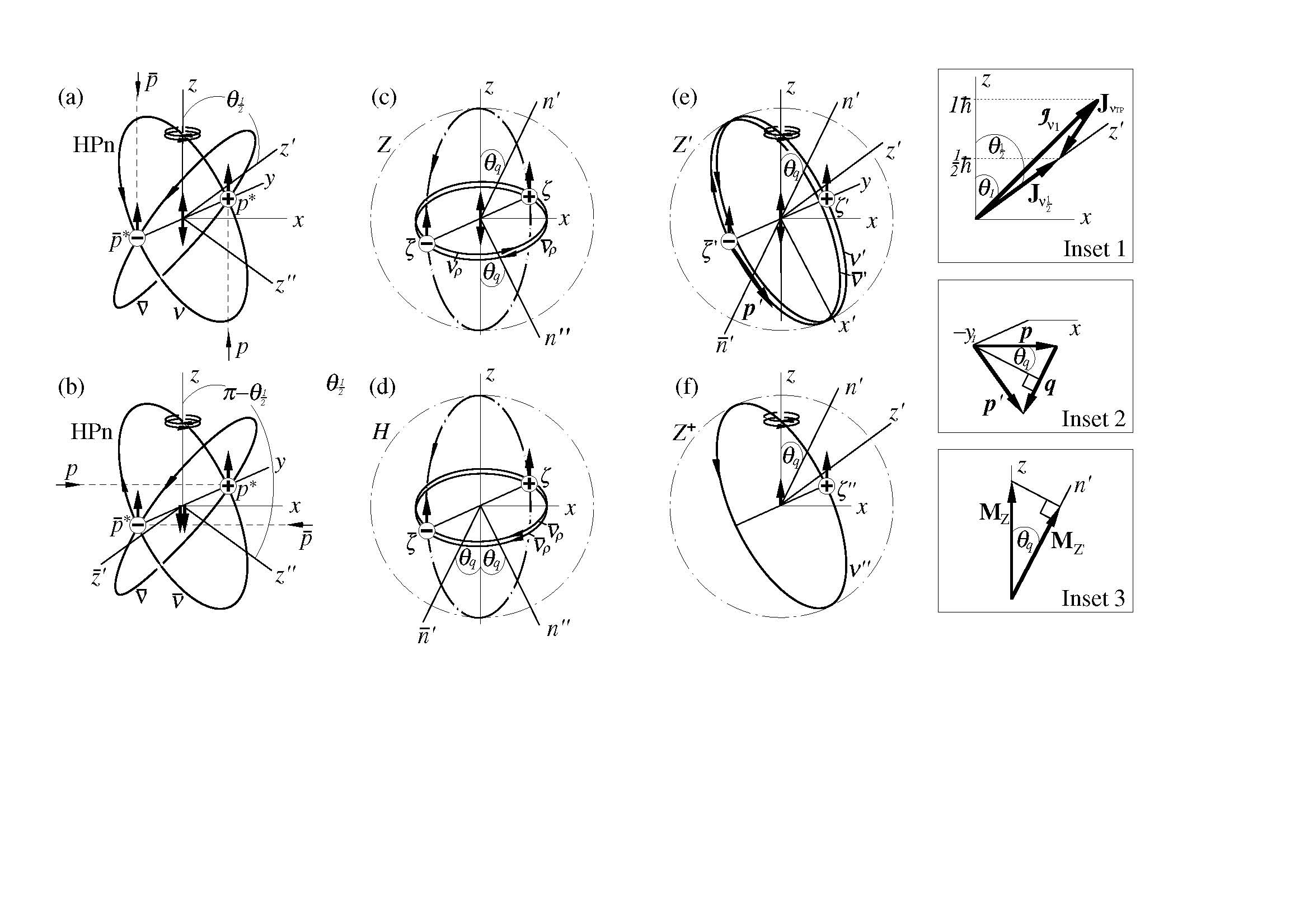
Figure 1: (a,b) Schematic structures of HPn’s composed each of $p^{*},{\bar{p}}^{*}$ in P-O motion along a two-orbit of $(\eta=)\nu,{\bar{\nu}}$ as produced by $p,{\bar{p}}$ incident along $+z,-z$ and n.h.o colliding at $+y_{1},-y_{1}$ on the $y$ axis in (a), and along ${\bar{\nu}},{\bar{\nu}}$ as produced by $p,{\bar{p}}$ incident along $+x,-x$ in (b). (c,d) The invariant rotated HPn’s, $Z(\zeta,{\bar{\zeta}})$, $H(\zeta,{\bar{\zeta}})$, with $\zeta,{\bar{\zeta}}$ on two-orbit of $(\eta_{\rho}=)\nu_{\rho},{\bar{\nu}}_{\rho}$ in (c) and ${\bar{\nu}}_{\rho},{\bar{\nu}}_{\rho}$ in (d) in the $xy$ plane. (e) The reverse invariant rotated $Z^{\prime}(\zeta^{\prime},{\bar{\zeta}}^{\prime})$ from $Z$, and (f) $Z^{\mbox{\tiny{$+$}}}(\zeta^{\prime\prime})$ as the positive charged state of $Z^{\prime}$. The $\nu/{\bar{\nu}},{\bar{\nu}}$ orbital normals $z^{\prime}/\bar{z}^{\prime},z^{\prime\prime}$ in (a)/(b) are at quantised angles $\theta_{\mbox{\tiny{$\frac{1}{2}$}}},\pi-\theta_{\mbox{\tiny{$\frac{1}{2}$}}}$ to $z$. The state vectors $\psi_{\eta}$ along $z^{\prime}/\bar{z}^{\prime},z^{\prime\prime}$ in (a)/(b) are rotated about $y$ by angles $-\theta_{q}=-\frac{1}{2}\theta_{\mbox{\tiny{$\frac{1}{2}$}}}$ to $\psi_{\eta}^{r}=\tilde{U}_{\mbox{\tiny{R}}}\psi_{\eta}$ along $n^{\prime}/\bar{n}^{\prime},n^{\prime\prime}$ in (c)/(d). The coherent components $\psi_{\eta_{\rho}}$ of $\psi_{\eta}^{r}$ along $+z,-z$ in (c) are rotated under $U_{\mbox{\tiny{R}}}=e^{-i\theta_{q}}$ by angles $\theta_{q}$ to along $n^{\prime},\bar{n}^{\prime}$ in (e). In (f), $\psi_{\nu^{\prime}}=U_{\mbox{\tiny{R}}}\psi_{\nu_{\rho}}$ is rotated from $\psi_{\nu_{\rho}}$ under $U_{\mbox{\tiny{R}}}$. Inset 1: The lab frame $\nu$ orbital angular momentum ${\bf{J}}_{\nu{\mbox{\tiny{$\frac{1}{2}$}}}}$ as the vector sum of the cmf term ${\boldsymbol{\mathcal{J}}}_{\nu 1}$ and a TP term ${\bf{J}}_{\nu{\mbox{{\tiny{$TP$}}}}}$. Inset 2: The rotation $U_{\mbox{\tiny{R}}}$ of $Z$ to $Z^{\prime}$ is illustrated as an elastic scattering of the ${\it{f\,}}$ particle of $Z$ incident with a linear momentum ${\bf{p}}=M_{\mbox{{\tiny{$Z$}}}}c\,{\bf x}$ parallel to $x$, into that of $Z^{\prime}$ of ${\bf{p}}^{\prime}=|{\bf{p}}|\,{\bf x}^{\prime}$ parallel to $x^{\prime}$ at angle $\theta_{\mbox{\tiny{$\frac{1}{2}$}}}$ from $x$; ${\bf{p}}^{\prime}=M_{\mbox{{\tiny{$Z$}}}}c\cos\theta_{q}\hat{{\bf{q}}}\times{\bf y}+\frac{1}{2}{\bf{q}}$, and $|{\bf{q}}|=|{\bf{p}}^{\prime}-{\bf{p}}|=2M_{\mbox{{\tiny{$Z$}}}}c\sin\theta_{q}$ is the momentum transfer. Inset 3: The $Z^{\prime}$ vector coherent mass ${\bf{M}}_{{\mbox{{\tiny{$Z$}}}}^{\prime}}$ in $\hat{{\bf{n}}}$ direction as cosine projected from the $Z$ mass ${\bf{M}}_{\mbox{{\tiny{$Z$}}}}$.

Finally, instead of the $Z$ production by the high energy $p,{\bar{p}}$ collision at the separation $\bar{r}_{2,1\rho}^{*}\sim 10^{-18}$ m, consider a low energy $e^{\mbox{-}}$ orbiting about $p$ (at rest) in the $xy$ plane say in orbital state $n,{\mbox{\scriptsize{$l$}}}=1,0$ at a separation $10^{-10}$ m at time $t=0$; choose the $p$ spin $s_{p}{\boldsymbol{\sigma}}=\frac{1}{2}{\boldsymbol{\sigma}}$ vector ${\boldsymbol{\sigma}}$ as the $z$ direction. Let the $e^{\mbox{-}}$ be then distablised, and firstly accelerated under the $e^{\mbox{-}}$-$p$ Coulomb force inward, first to a distance $r_{2,1(p)}^{0}=2\sqrt{2}r_{2(e)}^{0}/3\gamma{}_{ep}=2.17\times 10^{-13}$ m, where $\gamma{}_{ep}=M_{p}/M_{e}$, and $e^{\mbox{-}},p$ has a kinetic energy $T_{e}^{0}=\gamma{}_{ep}M_{e}c^{2}=M_{p}c^{2}$. Suppose that at about $r\lesssim r_{2,1(p)}^{0}$, $e^{\mbox{-}}$ experiences firstly a short range repulsion $F_{r}$ and then a short range attraction $F_{a}$ (the strong force origin proposition[5]), which form an energy barrier $\Delta V\sim-T_{e}^{0}$ that $e^{\mbox{-}}$ is just able to hop over to the low $r$ side. This $e^{\mbox{-}}$, denoting as $\beta{e}^{\mbox{-}}$, is thereof further accelerated (by $F_{a}$ and in turn by $-\partial V_{m}/\partial r^{*}$) in the $xy$ plane down to $\bar{r}_{2,1\rho}^{*}\sim 10^{-18}$ m, so swiftly that its initial energy $T_{e}^{0}(=M_{p}c^{2})=M_{\beta{e}^{\mbox{-}}}c^{2}$ manifests as a rest mass energy in one oscillation cycle, so that $p,\beta{e}^{\mbox{-}}$ become $\zeta,\beta{e}^{\mbox{-}}{}^{*}$ of a reduced mass ${\mathscr{M}}_{2,1\rho}^{*}=\gamma{}_{2,1}^{*}(\frac{1}{2}M_{p})\sqrt{\cos\theta_{q}}$, on orbit ${\bar{\nu}}_{\rho}$ in the $xy$ plane, mimicking that of $Z(\zeta,{\bar{\zeta}})$. The later further transition to $\zeta^{\prime},\beta{e}^{\mbox{-}}{}^{*}{}^{\prime}$ of a coherent mass $M_{{\mbox{{\tiny{$Z$}}}}^{\prime}}={\mathscr{M}}_{2,1\rho}^{*}{}^{\prime}$ (Sec D). The last is an eigen state satisfying the invariance of the final total angular momentum $J_{fz}=(s_{e}+s_{p}-j^{\prime})\hbar=\frac{1}{2}\hbar=J_{iz}$ versus the initial $J_{iz}=s_{p}\hbar$. So the P-O motion is about a single orbit $m_{j}^{\prime}=-j^{\prime}=-\frac{1}{2}$, or ${\bar{\nu}}^{\prime}$, as invariant rotated from ${\bar{\nu}}_{\rho}$. To the vacuum $\beta{e}^{\mbox{-}}{}^{*}{}^{\prime}$ remains to be $e^{\mbox{-}}$ of the rest mass $M_{e}$. The total reduced mass energy can be written ${\mathcal{E}}_{{\bar{\nu}}^{\prime}2,1\rho}^{\prime}=\hbar{\mathcal{K}}_{2,1\rho}^{\prime}c=\frac{\gamma{}_{2}^{*}{\mathscr{M}}_{2,1\rho}^{*\prime}\upsilon_{2}^{*2}}{\gamma{}_{2}^{*}+1}+\frac{\gamma{}_{ep}\frac{1}{2}\gamma{}_{ep}M_{e}\upsilon_{ep}^{2}}{\gamma{}_{ep}+1}+M_{e}c^{2}$. The total eigen function thus writes $\psi_{{\bar{\nu}}^{\prime}2,1\rho}^{r}=e^{-i{\mathcal{K}}_{2,1\rho}^{\prime}r^{*}}\dot{=}{\mit\Psi}_{{\bar{\nu}}^{\prime}2,1\rho}^{r}{\mit\Psi}_{ep}{\mit\Psi}_{e}$, the convolution of two fast oscillating ${\mit\Psi}_{{\bar{\nu}}^{\prime}2,1\rho}=e^{-ik_{{\bar{\nu}}2,1\rho}r^{*}}$, ${\mit\Psi}_{ep}=e^{-i\frac{\gamma{}_{ep}M_{e}c}{2\hbar}r^{*}}$ and a slow varying or essentially constant ${\mit\Psi}_{e}\dot{=}e^{-i\frac{M_{e}c}{\hbar}r^{*}}$. The process $e^{\mbox{-}}+p(\rightarrow\beta{e}^{\mbox{-}}+p)\rightarrow\beta{e}^{\mbox{-}}{}^{*}+\zeta+{\bar{\nu}}_{\rho}\rightarrow\beta{e}^{\mbox{-}}{}^{*\prime}+\zeta^{\prime}+{\bar{\nu}}^{\prime}$ represents a neutron $n$ production in terms of the $e^{\mbox{-}},p$ neutron model[5].

Appendix D $Z$, $H$ disintegrations. The intermediate mass states $Z^{\prime},Z^{\pm}$

If supplied with a threshold energy $H_{\mbox{\tiny{I}}}=-\bar{V}_{m}$ at time $t^{\prime}(=t-\tau)=0$, the bound $\zeta,{\bar{\zeta}}$ of $Z$ or $H$ tend to be distablised. These tend to separate apart by means of in situ down conversions to lighter particles so to obtain additional kinetic energy. $H$ has a similar structure to $Z$, and would on energy basis first down convert to $Z$, or the $Z^{\prime}$ later, and a mass state (denoting by $Z^{\dagger}$) due to the excess energy $E_{2,0}$. Our main subject henceforth is to formulate a formal down conversion, thereby disintegration scheme of $Z$ based on the charge dynamics and energy-momentum conditions of the component particles.

In general, $\zeta,{\bar{\zeta}}$ of charges $+e,-e$ would naturally first in situ down convert to two lighter mass states $\beta^{\prime},{\bar{\beta}}^{\prime}$ generated by the same charges $({\mathbin{q\mkern-11.0mu-}}=)+e,-e$ at the initial separation $\bar{r}_{2,1\rho}^{*}$, or to a lighter $\beta^{\prime}/{\bar{\beta}}^{\prime}$ and $A^{\pm}$ at rest depending on the activation symmetries. In the process the $\zeta,{\bar{\zeta}}$ charges, of initial oscillation displacements $\boldsymbol{\xi}_{\mathbin{q\mkern-11.0mu-}}=\xi_{\mathbin{q\mkern-11.0mu-}}\hat{{\mathbf{r}}}_{xy}$ each in level $N(=n_{\rm v}=1$ in $V_{{\rm v}+e}$ here) in $k$th orbital motion, can be generally regarded as first instantly retarded by ceasing the rotational oscillations. EMR fields are being emitted and re-absorbed, thereby re-driving the charges into oscillations of primed displacements $\boldsymbol{\xi}_{{\mathbin{q\mkern-11.0mu-}}}^{\prime}$ each in $N^{\prime}$th level in $k^{\prime}$th orbital motion, thereby forming $\beta^{\prime},{\bar{\beta}}^{\prime}$, of which one at least ought to be a stationary state (the principles of least action and maximum entropy [17]). For $\bar{r}_{2,1\rho}^{*}$ is of a similar dimension as the vacuum spacing $\sim 1\times 10^{-18}$ m, the charges are in effect situated in an isotropic potential field due either to $\bar{V}_{m}$ or $V_{\rm v}$. Their displacements can therefore have three equal probable orthogonal orientations, $\boldsymbol{\xi}_{{\mathbin{q\mkern-11.0mu-}}}^{\prime}=\xi_{{\mathbin{q\mkern-11.0mu-}}}^{\prime}{\bf x},\xi_{{\mathbin{q\mkern-11.0mu-}}}^{\prime}{\bf y},\xi_{\mathbin{q\mkern-11.0mu-}}^{\prime}{\bf{z}}$, thereby in theory generating three distinct pairs of $\beta^{\prime},{\bar{\beta}}^{\prime}$ equal probably, or similarly $\beta^{\prime}/{\bar{\beta}}^{\prime},A^{\mp}$.

Consider first the symmetric activation, and the re-driven oscillations of $+e,-e$ are along the radial directions along $y$ in Fig 1e, $\boldsymbol{\xi}_{{\mathbin{q\mkern-11.0mu-}}}^{\prime}=\xi_{{\mathbin{q\mkern-11.0mu-}}}^{\prime}{\bf y}$, as of the initial $Z(\zeta,{\bar{\zeta}})$. The final $\beta^{\prime},\bar{\beta}^{\prime}$ are implied to have internal P-O motions, or be of a ”weak” kind. As such, and for these to be separately stationary, $\zeta,{\bar{\zeta}}$ are stemmed to first adiabatic transform to two intermediate mass states $\zeta^{\prime},{\bar{\zeta}}^{\prime}$, comprising $Z^{\prime}$ of a reduced mass ${\mathscr{M}}^{*\prime}_{2,1\rho}=\frac{1}{2}M_{\zeta^{\prime}}$, that are in relative motions in egen orbital states given by the solutions to the SQR-KGE (Sec C). Moreover, their P-O angular momenta $J_{\eta^{\prime}j}=\sqrt{j^{\prime}(j^{\prime}+1)}\hbar$’s, need be invariant of the initial ${\bf{J}}_{\eta_{\rho}}$, and so are the totals. The minimals of such are the two P-O states $n^{\prime},{\mbox{\scriptsize{$l$}}}^{\prime},j^{\prime}=2,1,\frac{1}{2}$, $m_{j}^{\prime}=+\frac{1}{2},-\frac{1}{2}$, or denoting by $(\eta^{\prime}=)\nu^{\prime},{\bar{\nu}}^{\prime}$, which orbits remain coinciding and have opposite aligned normals $z^{\prime},\bar{z}^{\prime}$. Accordingly ${\bf{J}}_{\eta^{\prime}{\mbox{\tiny{$\frac{1}{2}$}}}}=\bar{{\mathbf{r}}}^{*}{}^{\prime}_{2,1\rho}\times({\mathscr{M}}^{*\prime}_{2,1\rho}{\mathbf{c}}^{\prime})=J_{\eta^{\prime}{\mbox{\tiny{$\frac{1}{2}$}}}}{\bf{z}}^{\prime}/\bar{{\bf{z}}}^{\prime}$, which are also desired invariant rotations from the initial ${\bf{J}}_{\eta_{\rho}}$ along $+z,-z$ to $z^{\prime},\bar{z}^{\prime}$ directions, by angles $\theta_{\mbox{\tiny{$\frac{1}{2}$}}}$ about the $y$ axis, such that their $z$ components are equal,

$$\halign{\hbox to\displaywidth{$\hfil\displaystyle#\hfil$}\cr 0.0pt{\hfil$\displaystyle\hfill\mbox{$J_{\pm\eta^{\prime}{\mbox{\tiny{$\frac{1}{2}$}}}z}(=\pm J_{\nu^{\prime}{\mbox{\tiny{$\frac{1}{2}$}}}}\cos\theta_{\mbox{\tiny{$\frac{1}{2}$}}})={\mathcal{J}}_{\pm\eta^{\prime}1z}\mp J_{\nu^{\prime}{\mbox{{\tiny{$TP$}}}}z}=\pm|\bar{r}^{*\prime}_{2,1\rho}\times{\mathscr{M}}_{\eta^{\prime}2,1\rho}^{*\prime}{\mathbf{c}}|\frac{1}{2}\cos\theta_{1}\equiv J_{\eta_{\rho}}=\pm\frac{1}{2}\hbar$}\hfill(\ref{eq-Jetaphfz})\crcr}}$$

The state vectors satisfying (D) are rotated under $U_{\mbox{\tiny{R}}}$ of (C) to $\psi_{\eta^{\prime}}^{r}=U_{\mbox{\tiny{R}}}\psi_{\eta_{\rho}}=e^{-i\theta_{q}}\psi_{\eta_{\rho}}$ along $n^{\prime},\bar{n}^{\prime}$ at angles $\theta_{q}$ to $+z,-z$. The masses described by $\psi_{\eta^{\prime}}^{r}$ are ${\mathscr{M}}_{\eta^{\prime}2,1\rho}^{*r}=e^{-i\theta_{q}}{\mathscr{M}}_{\eta 2,1\rho}^{*}={\mathscr{M}}_{\eta 2,1\rho}^{*}(\cos\theta_{q}-i\sin\theta_{q})$. The sine components, ${\mathscr{M}}^{*i.m}_{\eta 2,1\rho}=-i{\mathscr{M}}^{*}_{\eta 2,1\rho}\sin\theta_{q}$, are imaginary and associated with the pure rotations $U_{\mbox{\tiny{R}}}$ of the orbital normals from $z,-z$ to $n^{\prime},\bar{n}^{\prime}$. In the scattering description (Fig 1, Inset 2), the ${\mathscr{M}}^{*i.m}_{\eta 2,1\rho}$ are associated each with one half the momentum transfer ${\bf{q}}={\mathscr{M}}^{*}_{\eta 2,1\rho}c\sin\theta_{q}$ in the direction $n^{\prime}$ normal to the (instantaneous) rotation plane, (the averages of) which vector products with $\bar{{\mathbf{r}}}^{*\prime}_{2,1\rho}$ have a zero contribution to $J_{\pm\eta^{\prime}{\mbox{\tiny{$\frac{1}{2}$}}}z}$. The cosine projections ${\mathscr{M}}_{\eta^{\prime}2,1\rho}^{*\prime}={\mathscr{M}}_{\eta 2,1\rho}^{*}\cos\theta_{q}$ [cf Eq (Da) and Fig 1, Inset 3] are real and are coherent components rotating in the plane normal to $n^{\prime}$, and the mass vectors are defined in the positive $n^{\prime}$ direction. Their sum over $\eta^{\prime}=\nu^{\prime},{\bar{\nu}}^{\prime}$ gives the total (resonance) mass of $Z^{\prime}$ in (Da), and using this and $\bar{r}^{*\prime}_{2,1\rho}=\frac{\bar{r}^{*}_{2,1\rho}{\mathscr{M}}^{*}_{2,1\rho}}{{\mathscr{M}}^{*\prime}_{2,1\rho}(\frac{1}{2}\cos\theta_{1})}=\frac{\bar{r}^{*}_{2,1\rho}}{\cos\theta_{q}(\frac{1}{2}\cos\theta_{1})}=\frac{\bar{r}^{*}_{2,1}}{\sqrt{\cos\theta_{q}}\cos\theta_{q}}=4.90\times 10^{-18}$ m from (D) gives the real potential and interaction constant in (Db,c) below, with (C), (Cc) for $M_{\mbox{{\tiny{$Z$}}}}$, $\theta_{q}$,

$$\halign{\hbox to\displaywidth{$\hfil\displaystyle#\hfil$}\cr 0.0pt{\hfil$\displaystyle\hfill M_{{\mbox{{\tiny{$Z$}}}}^{\prime}}=\sum{}_{\eta^{\prime}}{\mathscr{M}}_{\eta^{\prime}2,1\rho}^{*\prime}={\mathscr{M}}_{2,1\rho}^{*}\cos\theta_{q}=M_{\mbox{{\tiny{$Z$}}}}\cos\theta_{q}=80.699\,{\rm GeV},\quad\bar{V}_{m2,1\rho}^{\prime}=-\frac{e^{2}\cos\theta_{q}}{4\pi\epsilon_{0}g_{2,1}\bar{r}^{*\prime}_{2,1\rho}}\hfill\cr 0.0pt{\hfil$\displaystyle\hfill=-\frac{G_{2,1\rho}^{\prime}}{\bar{{\mathscr{V}}}_{2,1}},\ \ G_{2,1\rho}^{\prime}=G_{2,1}\sqrt{\cos\theta_{q}}\cos^{2}\theta_{q}=\frac{4\sqrt{2}e^{2}\hbar^{2}c^{2}(\cos\theta_{q})^{\frac{11}{2}}}{3\epsilon_{0}M_{{\mbox{{\tiny{$Z$}}}}^{\prime}}^{2}c^{4}}=1.70\times 10^{-62}\,{\rm Jm}^{3}\hfill(\ref{eq-MZpGp})\crcr}}}$$

At essentially the same time $t^{\prime}=+0$ when their charges remain at $-y_{1},y_{1}$, the $\zeta^{\prime},{\bar{\zeta}}^{\prime}$ can proceed to in situ down transition to two final lower mass states $h^{\mbox{\tiny{$+$}}}_{\rho},h^{\mbox{-}}_{\rho}$, called a $(\rho\equiv)xy$ projected, heavy positron and electron in [6], generated by the charges $+e,-e$ of oscillations $\xi^{\prime}_{{\mathbin{q\mkern-11.0mu-}}{{\mbox{\tiny${N}$}}}^{\prime}(e)}=N^{\prime}{\cal{A}}_{{\mathbin{q\mkern-11.0mu-}}(e)}e^{-i{{\mit{\Omega}}}_{{\mathbin{q\mkern-11.0mu-}}(e)}t}$ in radial ($y$) directions in the $xy$ plane, in $N^{\prime}=1$th level in one half the difference potential field for each charge, $\Delta\bar{V}_{m2,1\rho}^{\prime}(\xi^{\prime}_{{\mathbin{q\mkern-11.0mu-}}1(e)})=\frac{1}{2}[V_{m2,1\rho}^{\prime}(\bar{r}^{*\prime}_{2,1\rho}+\xi^{\prime}_{{\mathbin{q\mkern-11.0mu-}}1(e)})-V_{m2,1\rho}^{\prime}(\bar{r}^{*\prime}_{2,1\rho})]=\frac{9G_{2,1\rho}^{\prime}\xi^{\prime}_{{\mathbin{q\mkern-11.0mu-}}1(e)}}{8\pi\bar{r}^{{}_{*}4}_{2,1}}\approx\frac{1}{2}\beta_{\mathbin{q\mkern-11.0mu-}}\xi_{{\mathbin{q\mkern-11.0mu-}}1(e)}^{\prime 2}$. Their rest masses ($M_{h_{\rho}}$’s) are determined by the level $N^{\prime}=1$ total mechanical energy (the g-IED model) $\frac{1}{2}{\mathfrak{M}}_{\mathbin{q\mkern-11.0mu-}}\dot{\xi}^{\prime 2}_{{\mathbin{q\mkern-11.0mu-}}1(e)}+\frac{1}{2}\beta_{\mathbin{q\mkern-11.0mu-}}\xi^{\prime 2}_{{\mathbin{q\mkern-11.0mu-}}1(e)}=\Delta\bar{V}_{m2,1\rho}^{\prime}({\cal{A}}_{{\mathbin{q\mkern-11.0mu-}}(e)})=\frac{9G_{2,1\rho}^{\prime}{\cal{A}}_{{\mathbin{q\mkern-11.0mu-}}(e)}}{8\pi\bar{r}^{{}_{*}4}_{2,1}}=M_{h_{\rho}}c^{2}$, where ${\mathfrak{M}}_{\mathbin{q\mkern-11.0mu-}}=\beta_{\mathbin{q\mkern-11.0mu-}}/{{\mit{\Omega}}}_{\mathbin{q\mkern-11.0mu-}}^{2}$. ${\cal{A}}_{{\mathbin{q\mkern-11.0mu-}}(e)}$ and hence $M_{h_{\rho}}$ are free parameters to be constrained by conforming to the energy of available lower stationary state in both the particle field and free vacuum in the sense discussed after (B). The latter is uniquely provided by a stationary HPs($e^{{\mbox{\tiny{$+$}}}*},e^{{\mbox{-}}*}$) in the minimal cmf orbital state $n^{\prime},{\mbox{\scriptsize{$l$}}}^{\prime}=2,1$ [6] of a rest reduced mass given using (B) for $a,\bar{a}=e^{\mbox{\tiny{$+$}}},e^{\mbox{-}}$ here (see further F), $\frac{1}{2}M_{h_{\rho}}={\mathscr{M}}_{2,1(e)}^{*}=\gamma{}_{2,1}^{*}\frac{1}{2}M_{e}$, or $M_{h_{\rho}}=\gamma{}_{2,1}^{*}M_{e}=\frac{3M_{e}}{2\alpha}=105.038$ MeV, and equilibrium orbital radius $\bar{r}_{2,1(e)}^{*}=2r_{2,1(e)}^{*}$, $r_{2,1(e)}^{*}=r_{2,1(e)}^{0}/\gamma{}_{2}^{*2}(=5.3248\times 10^{-15}$ m) given using (B). At the initial $\zeta^{\prime},{\bar{\zeta}}^{\prime}$ separation $\bar{r}_{2,1\rho}^{*\prime}$ here, $h_{\rho}^{\mbox{\tiny{$+$}}},h^{\mbox{-}}_{\rho}$ maintain opposite P-O motions at speeds $\upsilon^{\prime}=\sqrt{(\gamma{}^{\prime}{}^{2}-1)/\gamma{}^{\prime}{}^{2}}\,c\dot{=}c$ along the two coinciding partial orbits of states $n^{\prime},{\mbox{\scriptsize{$l$}}}^{\prime},j^{\prime}=2,1,\frac{1}{2},m_{j}^{\prime}=\frac{1}{2},-\frac{1}{2}$, or denoting by $(\eta_{e}=)\nu_{e},{\bar{\nu}}_{e}$ here, under momentum conservation conditions $\gamma{}^{\prime}{\mathscr{M}}_{\eta_{e}2,1(e)}^{*}\upsilon^{\prime}={\mathscr{M}}_{\eta^{\prime}2,1\rho}^{*\prime}c=\frac{M_{p}}{M_{e}}{\mathscr{M}}_{2,1(e)}^{*}\cos^{3/2}\theta_{q}$. This gives $\gamma{}^{\prime}=\frac{M_{p}}{M_{e}}\cos^{3/2}\theta_{q}$.

The transient, spatially oriented orbits $\nu_{e},{\bar{\nu}}_{e}$ are yet incompatible with the charge oscillations in the $xy$ plane. An explosive collision is hence prompted to produce two coinciding opposite energy currents in P-O states $n^{\prime\prime},{\mbox{\scriptsize{$l$}}}^{\prime\prime},j^{\prime\prime}=2,1,\frac{1}{2}$, $m_{j}^{\prime\prime}=-\frac{1}{2},+\frac{1}{2}$, or denoted by ${\bar{\nu}}_{\mu},\nu_{\mu}$. The ${\bar{\nu}}_{\mu},\nu_{\mu}$ orbital normals $z^{\prime\prime},\bar{z}^{\prime\prime}$ are opposite aligned at angles $\pi-\theta_{\mbox{\tiny{$\frac{1}{2}$}}},\theta_{\mbox{\tiny{$\frac{1}{2}$}}}$ to $z$, and are mirror reflections of $z^{\prime},\bar{z}^{\prime}$ about the $x$ axis. The final ($h_{\rho}^{\mbox{\tiny{$+$}}},\nu_{e},{\bar{\nu}}_{\mu})$, $(h_{\rho}^{\mbox{-}},{\bar{\nu}}_{e},\nu_{\mu})$, denoting by $\mu^{\mbox{\tiny{$+$}}},\mu^{\mbox{-}}$, are separately meta-stable, have charges $+e,-e$, spins $\frac{1}{2},\frac{1}{2}$, and each a rest mass $M_{\mu}=M_{h_{\rho}}+M_{\nu_{\mu}}+M_{\nu_{e}}\dot{=}105.29$ MeV ($M_{\nu_{\mu}}\dot{=}0.25$ MeV, $M_{\nu_{e}}\dot{=}0$ are used), and are in [6] identified as the observational muons of the measured masses 105.66 MeV each. Hence the $Z$ disintegration or decay equation $Z\rightarrow Z^{\prime}\rightarrow\mu^{\mbox{\tiny{$+$}}}+\mu^{\mbox{-}}$. For the $\mu^{\mbox{\tiny{$+$}}},\mu^{\mbox{-}}$ are in situ produced in the magnetic (or weak) potential $\bar{V}_{m2,1\rho}^{\prime}=-G_{2,1\rho}^{\prime}/\bar{{\mathscr{V}}}_{2,1}$ [Eq (Db,c)] field, the constant $G_{2,1\rho}^{\prime}$ can be compared with, though being larger than the Fermi constant $G^{exp}=1.4358\times 10^{-62}$ Jm³. Whilst the $G_{2,1\rho}^{\prime}$ value in (Dc) is an ab initio calculation, the $G^{exp}$ value is determined based on the life times of such particles as $\mu^{\mbox{-}}$, and also on the assumptions of complete wave function overlap, and a form factor 1 for point particle, which both tend to yield a smaller $G^{exp}$.

Consider secondly $\boldsymbol{\xi}_{\mathbin{q\mkern-11.0mu-}}^{\prime}=\xi_{\mathbin{q\mkern-11.0mu-}}^{\prime}{\mathbf{x}}$ and so are the ${\bf E}$ fields of their EMR along $x$, being transverse to their travel directions $+z,-z$ at $y_{1},-y_{1}$. The $\zeta,\bar{\zeta}$ can naturally in situ down convert a (relativistic) positron $e^{\mbox{\tiny{$+$}}}$ and electron $e^{\mbox{-}}$ generated by the charge $s+e,-e$ oscillations $\boldsymbol{\xi}_{{\mathbin{q\mkern-11.0mu-}}(e)}^{\prime}$, such that $e^{\mbox{-}}$ is a level $n_{\nu}=1$ stationary mass state in the vacuum potential $V_{{\rm v},-e}$ field to the charge $-e$ (the IED model). And the same mass for $e^{\mbox{\tiny{$+$}}}$ by pair production. Given the $H_{\mbox{\tiny{I}}}$ supplied, these are in effect un-bound here and able to travel off their orbit the opposite tangential directions parallel to $z,-z$. Hence the reaction $Z\rightarrow e^{\mbox{\tiny{$+$}}}+e^{\mbox{-}}$.

Consider thirdly $\boldsymbol{\xi}_{\mathbin{q\mkern-11.0mu-}}^{\prime}=\xi_{\mathbin{q\mkern-11.0mu-}}^{\prime}{\bf{z}}$ and so are the ${\bf E}$ fields of their EMR along $z$ directions. These are not radial, nor transverse to their rotational velocities at $y_{1},-y_{1}$. But the $\boldsymbol{\xi}_{\mathbin{q\mkern-11.0mu-}}^{\prime}$’s become radial when the charges have traveled (along orbits $\nu_{yz},{\bar{\nu}}_{yz}$) to $z_{1},-z_{1}$ on the $z$ axis. Here the down conversion can proceed to the final rotated states of $p_{2}$ (the level $n_{\rm v}=2$ mass state of charge $+e$ oscillation in the vacuum, of a rest mass $M_{p_{2}}=2M_{p}$) and ${\bar{p}}_{2}$, denoted by $\zeta_{2}^{0},{\bar{\zeta}}_{2}^{0}$ and called a rotated hyper-proton and hyper-antiproton, of the rest masses $M_{\zeta^{0}_{2}}=2M_{p}\sqrt{\cos\theta_{q}}=1768.5$ MeV each. At the in situ separation $\bar{r}_{2,1(p)}^{*}$, $\zeta_{2}^{0},{\bar{\zeta}}_{2}^{0}$ maintain spins $\frac{1}{2},\frac{1}{2}$ aligned along $z$, and in opposite P-O motions along two (rotated) coinciding orbits of states $n^{\prime},{\mbox{\scriptsize{$l$}}}^{\prime},j^{\prime}=4,1,\frac{1}{2}$, $m_{j}^{\prime}=\frac{1}{2},-\frac{1}{2}$, or denoting by $\nu_{p_{2}},{\bar{\nu}}_{p_{2}}$. The $n\rightarrow n^{\prime}$ transition is equi-separation, $\bar{r}_{4,1(p_{2})}^{*}=4\bar{r}_{1,1(p_{2})}^{*}=2\bar{r}_{1,1(p)}^{*}=\bar{r}_{2,1(p)}^{*}$, and equi-energy and momentum, with the $xy$-projected reduced mass ${\mathscr{M}}_{4,1\rho(p_{2})}^{*}=\gamma{}_{4,1}^{*}\times(\frac{1}{2}M_{\zeta^{0}_{2}})=\frac{3}{4\alpha}\times(\frac{1}{2}M_{p_{2}}\sqrt{\cos\theta_{q}})=\frac{3}{2\alpha}\times(\frac{1}{2}M_{p})\sqrt{\cos\theta_{q}}={\mathscr{M}}_{2,1\rho(p)}^{*}$. Similarly as the $Z\rightarrow\mu^{\mbox{\tiny{$+$}}},\mu^{\mbox{-}}$ process, two coinciding opposite energy currents ${\bar{\nu}}^{\prime\prime},\nu^{\prime\prime}$ are produced by an explosive collision. The final two separable quasi stationary components $\tau^{\mbox{\tiny{$+$}}}(p_{2},\nu_{{\mbox{\tiny{$+$}}}_{2}},{\bar{\nu}}^{\prime\prime})$, $\tau^{\mbox{-}}({\bar{p}}_{2},{\bar{\nu}}_{{\mbox{\tiny{$+$}}}_{2}},{\bar{\nu}})$, have charges $+e,-e$, spins $s_{\tau^{\mbox{\tiny{$+$}}}}(=s_{\zeta^{0}_{2}}+j-j),s_{\tau^{\mbox{-}}}=\frac{1}{2},\frac{1}{2}$, and rest masses $M_{\tau}=M_{\zeta^{0}_{2}}+M_{\nu_{p_{2}}}$ each. These properties and the $\tau^{\mbox{\tiny{$+$}}},\tau^{\mbox{-}}$ decay reactions (internal work) can be compared with those of the observational tau particles of measured masses $1784$ MeV each. Hence the decay reaction $Z\rightarrow\tau^{\mbox{\tiny{$+$}}}+\tau^{\mbox{-}}$.

Consider finally the asymmetric activation of $Z$ such that ${\bar{\zeta}}$ (or $\zeta$) is scattered into $A^{\mbox{-}}$ (or $A^{\mbox{\tiny{$+$}}}$) at rest, having effectively an infinite mass $M_{{\mbox{{\tiny{$A$}}}}}=\infty$; and its spin is in effects de-polarised. $\zeta$ (or ${\bar{\zeta}}$) alone assumes the total rotation of the cmf mass ${\mathscr{M}}_{2,1\rho}^{*}$ momentarily along a single orbit $\nu_{\rho}$ of radius $r_{\zeta}=r_{2,1\rho}^{*}$ about the $A^{\mbox{-}}$ (or $A^{\mbox{\tiny{$+$}}}$) at $r_{A}=0$. Similarly as the $Z\rightarrow Z^{\prime}$ process, $(\zeta,\nu_{\rho})$ subsequently first transform to an intermediate rotated state $Z^{\mbox{\tiny{$+$}}}(\zeta^{\prime\prime},\nu^{\prime\prime})$, see Fig 1f [or to $Z^{\mbox{-}}({\bar{\zeta}}^{\prime\prime},\nu^{\prime\prime})$]. $\zeta^{\prime\prime}/\bar{\zeta}^{\prime\prime}$ is re-generated by the charge $\pm e$ oscillation $\boldsymbol{\xi}_{\mathbin{q\mkern-11.0mu-}}^{\prime}=\xi_{\mathbin{q\mkern-11.0mu-}}^{\prime}{\bf y}$, and is in P-O motion about $A^{\mp}$ each in state $n^{\prime\prime},{\mbox{\scriptsize{$l$}}}^{\prime\prime},j^{\prime\prime},m_{j}^{\prime\prime}=2,1,\frac{1}{2},\frac{1}{2}$, or denoted by $\nu^{\prime\prime}$, with the orbital normal $z^{\prime}$ at angle $\theta_{\mbox{\tiny{$\frac{1}{2}$}}}$ to $z$. The P-O angular momentum, ${\bf{J}}_{\nu^{\prime\prime}{\mbox{\tiny{$\frac{1}{2}$}}}}=J_{\nu^{\prime\prime}{\mbox{\tiny{$\frac{1}{2}$}}}}{\bf{z}}^{\prime}$, is invariant of ${\bf{J}}_{\nu_{\rho}}$, such that $J_{\nu^{\prime\prime}{\mbox{\tiny{$\frac{1}{2}$}}}z}=J_{\nu_{\rho}z}=\frac{1}{2}\hbar$; hence the spin of $Z^{\pm}$ is $S_{{\mbox{{\tiny{$Z$}}}}^{\pm}}=s_{{\mbox{{\tiny{$Z$}}}}^{\pm}}\hbar=s_{\zeta^{\prime\prime}/{\bar{\zeta}}^{\prime\prime}}\hbar+\langle{\bf{J}}_{\nu^{\prime\prime}{\mbox{\tiny{$\frac{1}{2}$}}}}\rangle=(\frac{1}{2}+\frac{1}{2})\hbar=1\hbar$. The state vector is rotated under $U_{\mbox{\tiny{R}}}$ of (C) to the final $\psi_{\nu^{\prime\prime}}=e^{-i\theta_{q}}\psi_{\nu_{\rho}}$. The reduced mass of $Z^{\pm},A^{\mp}$ is ${\mathscr{M}}_{2,1\rho}^{*r}=e^{-i\theta_{q}}{\mathscr{M}}_{2,1\rho}^{*}$. Its cosine term gives the coherent reduced mass similarly as (Da), with $M_{{\mbox{{\tiny{$Z$}}}}^{\pm}}=M_{\zeta^{\prime\prime}}+M_{\nu^{\prime\prime}}\dot{=}M_{\zeta^{\prime\prime}}$,

$$\halign{\hbox to\displaywidth{$\hfil\displaystyle#\hfil$}\cr 0.0pt{\hfil$\displaystyle\hfill\frac{M_{\zeta}M_{\mbox{{\tiny{$A$}}}}}{M_{\zeta}+M_{\mbox{{\tiny{$A$}}}}}\dot{=}M_{{\mbox{{\tiny{$Z$}}}}^{\pm}}={\mathscr{M}}_{2,1\rho}^{*}\cos\theta_{q}=M_{{\mbox{{\tiny{$Z$}}}}^{\prime}}=80.699\ {\rm GeV}\hfill(\ref{eq-MZpm})\crcr}}$$

and the same $\bar{V}_{m2,1\rho}^{\prime},G_{2,1\rho}^{\prime}$ as given in (Db,c). Similarly, the final decay reactions are $Z^{\pm}\rightarrow\mu^{\pm}(h_{\rho}^{\pm},\nu_{e}/\bar{\bar{\nu}}_{e},{\bar{\nu}}_{\mu}/\nu_{\mu})+\nu_{\mu}/{\bar{\nu}}_{\mu}$, $e^{\pm}+\nu_{e}/{\bar{\nu}}_{e}$. In the last equation, ${\bar{\nu}}_{e}$ is the same (internal) spin up $\nu^{\prime\prime}$ energy current but travels off also in $+z$ direction (opposite to the $e^{\mbox{-}}$ travel $-z$ direction), having a helicity $+1$, hence the bar over $\nu_{e}$. Exceptionally the $\tau^{\pm}$ decay product channel is absent, apparently because the charge $\pm e$ on the single orbit $\nu^{\prime\prime}$ can never access $\pm z_{1}$ on the $z$ axis for a down conversion to $p_{2}/{\bar{p}}_{2}$ thereof. In sum, the theoretical $Z^{\mbox{\tiny{$+$}}},Z^{\mbox{-}}$ of charges $+e,-e$, spins $s_{{\mbox{{\tiny{$Z$}}}}^{\mbox{\tiny{$+$}}}},s_{{\mbox{{\tiny{$Z$}}}}^{\mbox{-}}}=1,1$ and the cmf masses given by (D) each can be compared with the observational charged IVB’s of measured (resonance) masses $80.377$ GeV[3] each.

Appendix E The SQR-KGE - The relativistic Schrördinger equation

Given a particle of rest mass $M$ traveling at linear velocity $\upsilon$ in a potential field $V$, the Klein-Goldon equation (KGE) is $[(E_{tot}-V)^{2}-M^{2}c^{4}]_{op}\psi_{tot}=p^{2}c^{2}\psi_{tot}$, where $E_{tot}=mc^{2}+V=E+Mc^{2}$ is the total Hamiltonian and $E=T+V=\frac{\gamma{}m\upsilon^{2}}{(\gamma{}+1)}+V$ the regular, $m=\gamma{}M$, $\gamma{}=[1-(\upsilon/c)^{2}]^{-1/2}$ or $\gamma{}^{2}-1$ $=\gamma{}^{2}(\upsilon/c)^{2}$, and $p^{2}=m^{2}c^{2}-M^{2}c^{2}=(\gamma{}^{2}-1)M^{2}c^{2}=\gamma{}^{2}(\frac{\upsilon^{2}}{c^{2}})^{2}M^{2}c^{2}=m^{2}\upsilon^{2}$. Adding $M^{2}c^{4}\psi_{tot}$ on both sides, the KGE becomes $[(E_{tot}-V)^{2}]_{op}\psi_{tot}=m^{2}c^{4}\psi_{tot}$. Or in the square root (SQR) form, $(E_{tot}-V)_{op}\psi=mc^{2}\psi$, where $\psi=\sqrt{\psi_{tot}}$. In turn adding $(-Mc^{2}+V)\psi$ on both sides, with $(E_{tot}-Mc^{2})_{op}=E_{op}$, $T_{op}=E_{op}-V=(\frac{\gamma{}m\upsilon^{2}}{\gamma{}+1})_{op}=\frac{\gamma{}(p^{2})_{op}r^{2}}{(\gamma{}+1)mr^{2}}$, and $mc^{2}-Mc^{2}+V=T+V=E$, we obtain the (reduced) SQR-KGE - or the relativistic Schrödiger equation,

$$\halign{\hbox to\displaywidth{$\hfil\displaystyle#\hfil$}\cr 0.0pt{\hfil$\displaystyle\hfill[\frac{\gamma{}(p^{2})_{op}r^{2}}{(\gamma{}+1)mr^{2}}+V]\psi=E\psi\hfill(\ref{sqr-kge})\crcr}}$$

For rotation, reserving $(p^{2})_{op}$ for the non-inertial rotational motion, and using $(p_{r}^{2})_{op}$ for an inertial radial motion, (E) becomes $[\frac{\gamma{}\left((p_{r}^{2})_{op}+(p^{2})_{op}\right)r^{2}}{(\gamma{}+1)mr^{2}}+V]\psi=E\psi$, the (reduced) SQR-KGE or relativistic Schrödinger equation used in the main text. This reduces to the non relativistic form $[\frac{1}{2M}\left((p^{2})_{op}+(p_{r}^{2})_{op}\right)+V]\psi=E\psi$ in the limit $\upsilon/c<<1$, $\gamma{}\dot{=}1$, $m\dot{=}M$.

Appendix F Errata for paper [6]

(i) In [6], the mass of $h^{\pm}_{\rho}$, $2\times{\mathscr{M}}^{*}_{2,1}$, (and similarly $2\times{\mathscr{M}}^{*}_{2}$ of $h^{\pm}$), was inappropriately argued to result from a double energy level of the HPs (hence DHPs) that would be physical only if the two energy quanta that are both formed and observed in the cmf. (ii) The exact total mass energy of the ${\it{f\,}}$ particle of $e^{{\mbox{\tiny{$+$}}}*},e^{{\mbox{-}}*}$ is ${\mathscr{M}}_{2,1(e)}^{*}c^{2}$ as given using (B), hence $M_{h_{\rho}}=2{\mathscr{M}}_{2,1(e)}^{*}$. The $M_{h_{\rho}}$ mass ($2{\mathscr{M}}_{2,1(e)}^{*}+M_{e}$) given in [6] incorrectly contains a term $M_{e}$.

References

References

[1]
Nakamuura K et al (Particle Data Group) 2010
J. Phys. G: Nucl. Part. Phys.37 075021;
P J Mohr 2008 CODATA recommend values of the fundamental physical constants: 2006” Rev. Mod. Phys.80, 633-730;
D. Griffith 1987 Introduction to elementary particles (Harper and Row Publisher);
D Brune, B Forkman, B Persson 1984 Nuclear Analytical Cemetery (Studentlitteratur, Lund);
E Rutherford 1919 Phil. Mag.37 581;
J J Thomson 1897 Phil Mag44 293.
[2] Zheng-Johansson J. X. and P-I. Johansson 2006
Unification of Classical, Quantum and Relativistic Mechanics and of the Four Forces (Nova Sci. Pub. Inc., N. Y.).
Zheng-Johansson, J.X. 2003
Unification of Classical and Quantum Mechanics & The Theory of Relative Motion
Bullet Amer. Phys. Soc.G35.001 General Physics, March; Zheng-Johansson, J.X., P-I Johansson, (Feb 24) 2003
Unification Scheme for Classical and Quantum Mechanics at All Velocities (I) fundamental construction of material particles, submitted to Proc Roy Soc Lond..
[3]
Zheng-Johansson, J. X. 2006
Inference of Basic Laws of Classical, Quantum and Relativistic Mechanics from First-Principles Classical-Mechanics Solutions (Nova Sci. Pub., Inc., N. Y.).
[4] Zheng-Johansson J. X. and P.-I. Johansson 2006 Inference of Schrödinger equation from classical mechanics solution
Suppl. Blug. J. Phys. 33, 763,
Quantum Theory and SymmetriesIV.2,
ed. V.K. Dobrev (Heron Press, Sofia), p763
(Preprint arxiv:physics/0411134v5).
[5] Zheng-Johansson J. X. and P.-I. Johansson 2006 Developing de Broglie wave Prog. Phys. 4, 32
(Preprint arxiv:physics/0608265).
[6] Zheng-Johansson J. X. and P.-I. Johansson 2006 Mass and mass–energy equation from classical-mechanics solution
Phys. Essays 19, 544 (Preprint
arxiv:physics/0501037).
[8]
Zheng-Johansson J. X. 2008
Dirac equation for electrodynamic model particles J. Phys: Conf. Series128, 012019, Proc. 5th Int. Symp. Quantum Theory and Symmetries, ed. M. Olmo (Valladolid, 2007).
[9] Zheng-Johansson J. X. 2007 Vacuum structure and potential
Preprint arxiv:0704.0131.
[10]
Zheng-Johansson J. X. 2006 Dielectric theory of the vacuum,
Preprint arxiv:physics/0612096.
[11]
Zheng-Johansson J. X., P.-I. Johansson, R. Lundin 2006 Depolarisation radiation force in a dielectric medium. its analogy with gravity, Suppl. Blug. J. Phys.33, 771;
J. X. Zheng-Johansson and P.-I. Johansson, Gravity between internally electrodynamic Particles, Preprint arxiv:physics/0411245.
[12] Zheng-Johansson J. X. 2008 Doebner-Goldin Equation for electrodynamic model particle. The implied applications Preprint arxiv:0801.4279,
Talk at 7th Int. Conf. Symm. in Nonl. Math. Phys. (Kyiv, 2007).
[13]
Zheng-Johansson J. X. 2010 Internally electrodynamic particle model: its experimental basis and its predictions Phys. Atom. Nucl.73 571-581 (Preprint arxiv:0812.3951), Proc Int 27th Int Colloq Group Theory in Math Phys. ed. G Pogosyan (Ireven, 2008).
[14] Zheng-Johansson
2010 Self interference of single electrodynamic particle in double slit Preprint arxiv:1004.5000; Talk at Proc. 6th Int. Symp. Quantum Theory & Symm.
(Lexington, 2009).
[15] Zheng-Johansson J. X. 2010 Quantum-Mechanical Probability of IED Particle(s) Preprint arxiv: 1011.1344. Talk at 28th Int. Colloq. Group Theory in Math. Phys. (Newcastle, 2010).
[16] Zheng-Johansson J. X. 2011
Intermediate Emission Process of Radiation Quantum (internal).
[17]
The experimentally measured upper bound of electromagnetic radiation frequency is
1/s (see e.g. C Nordling and J Österman, Physics Handbook for Sci Eng, 6th Ed, Studentlitteratur, 1999, p53, Table 4.2); this gives the minimum wavelength m. A vacuum continuum able to propagate the electromagnetic wave, regarded as an elastic wave in the vacuum continuum, of this shortest-wavelength should have a spacing at least several times smaller than . Taking the scaling factor to be 6 here, we have m.
[18] Merzbacher E. 1970 Quantum Mechanics (John Wiley and Sons, Inc.) p. 57; L I Schiff, qunatum mechnics, 3rd edn, (McGraw-Hill Book Company, New York, 1968) p71
[19] Zheng-Johansson J. X. 2011
Inference of the Constancy of Planck Constant and the Equal a Priori Probabilities from First Principles (internal).

References

[1]
(a) Perkins DH 1982 Introduction to High Energy Physics, 2nd ed (Reading: Addison-Wesley);
(b) Griffiths D 1987 Introduction to elementary particles (New York: Harper
& Row);
(c) Williams WSC 1992 Nuclear and Particle Physics (Oxford: Clarendon);
(d) Enge HA 1969 Introduction to Nuclear Physics (Massachusetts: Addison-Wesley);
(e) Beringer J, et al (Particle Data Group) 2012 Phys. Rev.D86 010001;
(f) Alvarez L and Bloch H 1940
Phys Rev57 111;
Staub HH and Roger EH 1950
Hel Phys Acta23 63-92.
[2]
(a) Higgs P 1964
Phys. Lett.12 132;
1964 Phys. Rev. Lett.13 508-9; ibid 321;
Englert P and Brout R 1964 Phys. Rev. Lett.13 321;
Gutranik GS, Hagen CR and Kibble TWB 1964 Phys. Rev. Lett.13 585;
(b) Weinberg S 1967
Phys. Rev. Lett.19 1264;
Salam A 1968 in Elementary particle physics: relativistic groups and analicity, Nobel Symp.8, Svartholm N ed (Stockholm: Almquist & Wiksells) p 367;
(c) Glashow SL, Lliopoulos L and Maiani I 1970 Phys. Rev.D2 1285;
(d) ’T Hooft G 1971
Nucl. Phys.B33 173-99;
1971 Phys. Lett.B37 195; (e) Fermi E 1934
Zeit. f. Physik88171;
tr Wilson FL 1968 Am. J. Phys.36 1150-60.

References

[1] Perkins DH 2000 Introduction to High Energy Physics, 4th ed (Cambridge: Cambridge University Press)
[2] Frauenfelder H and EM Henley 1991 Subatomic Physics 2nd ed (New Jersey: Prentice-Hall)
[3] Zheng-Johansson JX 2010
Internally electrodynamic particle model: its experimental basis and its predictions,
Phys Atom Nucl73 571-81 Proc 27th Int Group Theo Meth Phys ed G Pogosyan (Irevan 2008) (Preprint arxiv:0812.3951).
[4]
Zheng-Johansson JX 2006 Dielectric theory of vacuum Preprint arXiv:physics/0612096.
[5]
Zheng-Johansson JX and P-I Johansson 2006
Unification of Classical, Quantum and Relativistic Mechanics and of the Four Forces (New York: Nova Science).
[6] Zheng-Johansson JX 2012
Vacuum potentials for the two only permanent free particles, proton and electron.
J Phys Conf Ser343 012135 Proc Int Quant Theo & Symm ed C Burdik (Prague 2011) (Preprint arxiv1111.3123)
[7]
Zheng-Johansson JX 2016 A microscopic theory of the neutron J Phys Conf Ser670 012056 23rd Int Conf Integ Sys Quant Symm ISQS23, ed C Burdik (Prague 2015).
[8] Jackson JD 1999 Classical Electrodynamics, 3rd ed (New York: John Willey and Sons)

References

[1] Perkins DH 2000 Introduction to High Energy Physics 4th ed (Cambridge: Cambridge University),
1982 ibid
2nd ed (Reading: Addison-Wesley)
[2] H Frauenfelder and EM Henley 1991 Subatomic Physics 2nd ed (New Jersey: Prentice-Hall)
[3]
Workman RL et al (Particle Data Group) 2022 Prog. Theor. Exp. Phys2022 083C01
[4] Zheng-Johansson JX 2010 Internally Electrodynamic Particle Model: Its Experimental Basis and Its Predictions, Phys. Atom. Nucl.73, 571-81 Proc 27th Int Group Theoretical Method in Physics, Yrevan, 2008 (Preprint arxiv:0812.3951)
[5] Zheng-Johansson JX 2016 A microscopic theory of the neutron, J. Phys.: Conf. Ser.670 012056
[6] Zheng-Johansson JX 2019 A Quantum Electromagnetic Theory of the Muons, Pions, and Their Emitting Particles (I) J. Phys.: Conf. Ser.1416 012043 Proc Int Conf Integ Sys & Quant Symm ISQS, Prague, 2019
(Preprint arXiv:1111.3123, Part C)
[7] Zheng-Johansson JX 2006 Dielectric Theory of Vacuum (preprint) arXiv:physics/0612096
[8]Zheng-Johansson JX, Johansson P-I 2005
Unification of Classical, Quantum and Relativistic Mechanics and of the Four Forces (New York: Nova Science)
[9] Zheng-Johansson JX 2012 Vacuum Potentials for the Two Only Permanent Free Particles, Proton and Electron. Pair Productions, J. Phys Conf Series343 012135 (Preprint arxiv1111.3123)
[10] Zheng-Johansson JX, P-I Johansson 2006 Mass and mass energy relation from classical-mechanics solution Physics Essays19 544-552 (Preprint arXiv:physics/0501037)
[11] UA1 Collaboration (CERN) 1983
Experimental observations of lepton pairs of invariant mass around 95 GeV at the CERN SPS collider
Phys Letters126B 398-410
[12]
UA1 Collaboration (CERN) 1983
Experimental observations of isolated large transverse energy electrons with associated missing energy at 540 GeV
Phys Letters122B 103-116
[13]
Atlas Collab 2012
Observation of a new particle in the search for the standard model Higgs boson with the ATLAS detector at the LHC Phys LettB 716 1-29
[14] Merzbacher E 1988 Quantum mechanics, 3ed (New York: John Wiley & Sons, Inc.)
[15] Schiff LI 1968 Quatum mechanics 3ed
(London: McGraw-Hill)
[16] Jackson JD 1999 Classical Electrodynamics, 3rd ed (New York: John Wiley and Sons)
[17] Zheng-Johansson JX 2019
Inference of the universal constancy of Planck constant based on first principlesJ. Phys.: Conf. Ser.1194 012119
Proc Int Colloq Group Theo Meth Phys, Prague 2019
Note: The References for Part D either appear twice, or they do not appear, due apparently to a bug entering the laTex compilation, not due to typo error in my manuscript.