Medians and means in Riemannian geometry: existence, uniqueness and computation

Abstract

This paper is a short summary of our recent work on the medians and means of probability measures in Riemannian manifolds. Firstly, the existence and uniqueness results of local medians are given. In order to compute medians in practical cases, we propose a subgradient algorithm and prove its convergence. After that, Fréchet medians are considered. We prove their statistical consistency and give some quantitative estimations of their robustness with the aid of upper curvature bounds. We also show that, in compact Riemannian manifolds, the Fréchet medians of generic data points are always unique. Stochastic and deterministic algorithms are proposed for computing Riemannian $p$-means. The rate of convergence and error estimates of these algorithms are also obtained. Finally, we apply the medians and the Riemannian geometry of Toeplitz covariance matrices to radar target detection.

1 Introduction

It has been widely accepted that the history of median begins from the following question raised by P. Fermat in 1629: given a triangle in the plan, find a point such that the sum of its distances to the three vertices of the triangle is minimum. It is well known that the answer to this question is: if each angle of the triangle is smaller than $2\pi/3$, then the minimum point is such that the three segments joining it and the vertices of the triangle form three angles equal to $2\pi/3$; in the opposite case, the minimum point is the vertex whose angle is no less than $2\pi/3$. This point is called the median or the Fermat point of the triangle.

The notion of median also appears in statistics since a long time ago. In 1774, when P. S. Laplace tried to find an appropriate notion of the middle point for a group of observation values, he introduced “the middle of probability”, the point that minimizes the sum of its absolute differences to data points, this is exactly the one dimensional median used by us nowadays.

A sufficiently general notion of median in metric spaces was proposed in 1948 by M. Fréchet in his famous article [23], where he defined a $p$-mean of a random variable $X$ to be a point which minimizes the expectation of its distance at the power $p$ to $X$. This flexible definition allows us to define various typical values, among which there are two important cases: $p=1$ and $p=2$, corresponding to the notions of median and mean, respectively.

Apparently, the median and mean are two notions of centrality for data points. As a result, one may wonder that which one is more advantageous? Statistically speaking, the answer to this question depends on the distribution involved. For example, the mean has obvious advantage over the median when normal distributions are used. On the contrary, as far as Cauchy distributions are concerned, the empirical mean has the same accuracy as one single observation, so that it would be better to use the median instead of the mean in this situation. Perhaps the most significant advantage of the median over the mean is that the former is robust but the latter is not, that is to say, the median is much less sensitive to outliers than the mean. Roughly speaking, in order to move the median of a group of data points to arbitrarily far, at least a half of data points should be moved. Oppositely, in order to move the mean of a group of data points to arbitrarily far, it suffices to move one data point. So that medians are in some sense more prudent than means, as argued by M. Fréchet. The robustness property makes the median an important estimator in situations when there are lots of noise and disturbing factors.

The first formal definition of means for probability measures on Riemannian manifolds was made by H. Karcher in [24]. To introduce Karcher’s result concerning means, consider a Riemannian manifold $M$ with Riemannian distance $d$ and

$$B(a,\rho)=\{x\in M:d(x,a)<\rho\}$$

is a geodesic ball in $M$ centered at $a$ with a finite radius $\rho$. Let $\Delta$ be an upper bound of sectional curvatures in $\bar{B}(a,\rho)$ and $\mathop{\rm inj}\nolimits$ be the injectivity radius of $\bar{B}(a,\rho)$. Under the following condition:

$$\rho<\min\big{\{}\mskip 3.0mu\frac{\pi}{4\sqrt{\Delta}}\mskip 3.0mu,\mskip 3.0mu\frac{\mathop{\rm inj}\nolimits}{2}\mskip 3.0mu\big{\}},$$ (1)

where if $\Delta\leq 0$, then $\pi/(4\sqrt{\Delta})$ is interpreted as $+\infty$, Karcher showed that, with the aid of estimations of Jacobi fields, the local energy functional

$$F_{\mu}:\quad\bar{B}(a,\rho)\longrightarrow\mathbf{R}_{+},\quad x\longmapsto\int_{M}d^{2}(x,p)\mu(dp)$$ (2)

is strictly convex, thus it has a unique minimizer $b(\mu)$, which he called the Riemannian center of mass of the probability measure $\mu$. Moreover, $b(\mu)$ is also the unique solution of the following equation:

$$\int_{M}\exp_{x}^{-1}p\mskip 3.0mu\mskip 3.0mu\mu(dp)=0_{x},\quad x\in\bar{B}(a,\rho).$$ (3)

From then on, local means of probability measures on Riemannian manifolds are also called Karcher means, meanwhile, global means are often called Fréchet means. A rather general result concerning the uniqueness of local means was proved by W. S. Kendall in [25]. As a particular case of Kendall’s result, the condition

$$\rho<\frac{1}{2}\min\big{\{}\mskip 3.0mu\frac{\pi}{\sqrt{\Delta}}\mskip 3.0mu,\mskip 3.0mu\mathop{\rm inj}\nolimits\mskip 3.0mu\big{\}}$$ (4)

is sufficient to ensure the uniqueness of the Kacher means of $\mu$.

Some generalizations of Karcher mean are given by many authors. For instance, M. Emery and G. Mokobodzki defined in [21] the exponential barycenters and convex barycenters for measures on affine manifolds. They also showed that a point $x$ is a convex barycenter of a probability $\mu$ if and only if there exists a continuous martingale starting from $x$ with terminal law $\mu$. The uniqueness of exponential barycenters are generalized by M. Arnaudon and X. M. Li in [3] to probability measures on convex affine manifolds with semilocal convex geometry. Moreover, the behavior of exponential barycenters when measures are pushed by stochastic flows is also considered in [3]. In order to study harmonic maps between Riemannian manifolds with probabilistic methods, J. Picard also gave a generalized notion of barycenters in [27]. As we noted before, Karcher means are only local minimizers of the energy functional $f_{\mu}$ in (2), but it is easily seen that $f_{\mu}$ can be defined not only on the closed ball $\bar{B}(a,\rho)$ but also on the whole manifold $M$ as long as the second moment of $\mu$ is finite. This leads to the global minimizers of the second moment function of $\mu$, which is just the original definition of means made by Fréchet. Global minimizers are more useful in statistics than local ones, so that it is necessary to know whether or under which conditions the Karcher mean of $\mu$ is in fact the Fréchet mean. For the case when $\mu$ is a discrete measure supported by finitely many points in the closed upper hemisphere, S. R. Buss and J. P. Fillmore showed in [17] that if the support of $\mu$ is not totally contained in the equator then $\mu$ has a unique Karcher mean which lies in the open hemisphere and equals to the Fréchet mean. Inspired by the methods of Buss and Fillmore, B. Afsari showed in [1] that if the upper curvature bound $\Delta$ and the injectivity radius $\mathop{\rm inj}\nolimits$ in (4) is replaced by the ones of the larger ball $B(a,2\rho)$, then all the Fréchet $p$-means of $\mu$ lie inside $B(a,\rho)$. Particularly, the Karcher mean coincides with the Fréchet mean. The existence and uniqueness of $p$-means in Finsler geometry are recently proved by M. Arnaudon and F. Nielsen in [6]. They also showed that Finslerian $p$-means are limiting points of continuous gradient flows and developed algorithms for computing $p$-means in Finsler geometry.

Medians of discrete sample points on the sphere are studied by economists and operational research experts in the 1970s and 1980s, but they used the name “location problems on a sphere”. For data points lying in a spherical disc of radius smaller than $\pi/4$, Drezner and Wesolowsky showed in [19] that the cost function is unimodal in that disc and the Fréchet median is unique if the data points are not contained in a single great circle. It is also shown by Z. Drezner in [20] that if all the sample points are contained in a great circle, then one of the sample points will be a Fréchet median. Perhaps the first work about Fréchet medians on Riemannian manifolds is the paper [26] by R. Noda and his coauthors. They proved the uniqueness, characterizations and position estimations of Fréchet medians for discrete sample points lying in a Cartan-Hadamard manifold. In order to do robust statistics for data living in a Riemannian manifold P. T. Fletcher and his coauthors defined in [22] the local medians for discrete sample points and showed their existence and uniqueness.

In this paper, we present our results on medians and means of probability measures in Riemannian manifolds. Above all, the motivation of our work: radar target detection is introduced in section 2. After that, in section 3 we define local medians for probability measures in Riemannian manifolds and consider the problems of uniqueness and approximation. Under the assumption that the support of the probability measure is contained in a convex ball, we give some results on the characterization, the position estimation and the uniqueness of medians. Then we propose a subgradient algorithm to estimate medians as well as giving its convergence result without condition of the sign of curvatures. Our algorithm improves the one proposed in [22] which is shown to be convergent only if the manifold is nonnegatively curved. Finally, the problem of error estimation and rate of convergence are also considered.

The aim of section 4 is to give some basic properties of Fréchet medians of probability measures in Riemannian maniolds. Firstly, we give the consistency result of Fréchet medians in proper metric spaces. Particularly, if a probability measure has only one Fréchet median, then any sequence of empirical Fréchet medians will converge almost surely to it. After that, we study the robustness of Fréchet medians in Riemannian manifolds. It is well known that in Euclidean spaces, if a group of data points has more than a half concentrated in a bounded region, then its Fréchet median cannot be drown arbitrarily far when the other points move. A generalization and refinement of this result for data points in Riemannian manifolds is given in Theorem 4.3. This theorem also generalizes a result in [1] which states that if the probability measure is supported in a strongly convex ball, then all its Fréchet medians lie in that ball. At the end of this section, the uniqueness question of Fréchet sample medians is considered in the context of compact Riemannian manifolds. It is shown that, apart from several events of probability zero, the Fréchet sample medians are unique if the sample vector has a density with respect to the canonical Lebesgue measure of the product manifold. In other words, the Fréchet medians of generic data points are always unique.

Section 5 is devoted to presenting algorithms for computing Fréchet $p$-means in order to meet practical needs. Theorem 5.1 gives stochastic algorithms which converge almost surely to $p$-means in manifolds, which are easier to implement than gradient descent algorithm since computing the gradient of the function to minimize is not needed. The idea is at each step to go in the direction of a point of the support of $\mu$. The point is chosen at random according to $\mu$ and the size of the step is a well chosen function of the distance to the point, $p$ and the number of the step. The speed of convergence is given by Theorem 5.2, which says that the renormalized inhomogeneous Markov chain of Theorem 5.1 converges in law to an inhomogeneous diffusion process. We give the explicit expression of this process, as well as its local characteristic. After that, the performance of the stochastic algorithms are illustrated by simulations. Finally, we show that the $p$-mean of $\mu$ can also be computed by the method of gradient descent. The questions concerning the choice of stepsizes and error estimates of this deterministic method are also considered. We note that, for the case when $p=+\infty$, M. Arnaudon and F. Nielsen developed in [5] an efficient algorithm to compute the circum-center $e_{\infty}$ of probability measures in Riemannian manifolds.

In section 6, we consider the manifold of $n\times n$ Toeplitz covariance matrices parameterized by the reflection coefficients which are derived from Levinson’s recursion of autoregressive models. The explicit expression of the reparametrization and its inverse are obtained. With the Riemannian metric given by the Hessian of a Kähler potential, we show that the manifold is in fact a Cartan-Hadamard manifold with lower sectional curvature bound $-4$. After that, we compute the geodesics and use the subgradient algorithm introduced in section 3 to find the median of Toeplitz covariance matrices. Finally, we give some simulated examples to illustrate the application of the median method to radar target detection.

2 Motivation: radar target detection

Suggested by J. C. Maxwell’s seminal work on electromagnetism, H. Hertz carried out an experiment in 1886 which validated that radio waves could be reflected by metallic objects. This provided C. Hüelsmeyer the theoretical foundation of his famous patent on “telemobiloscope” in 1904. He showed publicly in Germany and Netherlands that his device was able to detect remote metallic objects such as ships, even in dense fog or darkness, so that collisions could be avoided. Hüelsmeyer’s “telemobiloscope” is recognized as the primogenitor of modern radar even though it could only detect the direction of an object, neither its distance nor its speed. This is because the basic idea of radar was already born: send radio waves in a predetermined direction and then receive the possible echoes reflected by a target. In order to know the distance and the radial speed of the target, it suffices to send successively two radio waves. In fact, it is easily seen that the distance $d$ of the target can be computed by the formula

$$d=\frac{c\Delta t}{2},$$

where $c$ is the speed of light and $\Delta t$ is the time interval between every emission and reception in the direction under test. Moreover, the radial speed $v$ of the target can be deduced by the Doppler effect which states that the frequency of a wave is changed for an observer moving relatively to the source of the wave. More precisely,

$$v=\frac{\lambda\Delta\varphi}{4\pi\Delta t},$$

where $\lambda$ and $\Delta\varphi$ are the wavelength and the skewing of the two emitted radio waves, respectively. As a result, the direction, the distance and the speed of the target can all be determined.

For simplicity, from now on we only consider a fixed direction in which a radar sends radio waves. Since the range of emitted waves are finite, we can divide this direction into some intervals each of which represents a radar cell under test. The radar sends each time a rafale of radio waves in this direction and then receive the returning echoes. For each echo we measure its amplitude $r$ and phase $\varphi$, so that it can be represented by a complex number $z=re^{i\varphi}$. As a result, the observation value of each radar cell is a complex vector $Z=(z_{1},\dots,z_{N})$, where $N$ is the number of waves emitted in each rafale.

The aim of target detection is to know whether there is a target at the location of some radar cell in this direction. Intuitively speaking, a target is an object whose behavior on reflectivity or on speed is very different from its environment. The classical methods for target detection is to compute the difference between the discrete Fourier transforms of the radar observation values of the cell under test and that of its ambient cells. The bigger this difference is, the more likely a target appears at the location of the cell under test. However, the performance of these classical methods based on Doppler filtering using discrete Fourier transforms together with the Constant False Alarm Rate (CFAR) is not very satisfactory due to their low resolutions issues in perturbed radar environment or with smaller bunch of pulses.

In order to overcome these drawbacks, a lot of mathematical models for spectra estimation were introduced, among which the method based on autoregressive models proposed by F. Barbaresco in [7] is proved to be very preferable. We shall introduce this method in Chapter 6 of this dissertation. The main difference between this new method and the classical ones is that, instead of using directly the radar observation value $Z$ of each cell, we regard it as a realization of a centered stationary Gaussian process and identify it to its covariance matrix $R=\mathbf{E}[ZZ^{*}]$. Thus the new observation value for each radar cell is a covariance matrix which is also Toeplitz due to the stationarity of the process. As a result, the principle for target detection becomes to find the cells where the covariance matrix differs greatly from the average matrix of its neighborhood. Once such cells are determined we can conclude that there are targets in these locations. In order to carry out this new method, there are two important things which should be considered seriously. One is to define a good distance between two Toeplitz covariance matrices. The other is to give a reasonable definition of the average of covariance matrices, which should be robust to outliers so as to be adapted to perturbed radar environment, and develop an efficient method to compute it in practical cases. These works will be done in the following by studying the Riemannian geometry of Toeplitz covariance matrices and the medians of probability measures in Riemannian manifolds.

3 Riemannian median and its estimation

In this section, we define local medians of a probability measure on a Riemannian manifold, give their characterization and a natural condition to ensure their uniqueness. In order to compute medians in practical cases, we also propose a subgradient algorithm and show its convergence. The mathematical details of this section can be found in [31].

In more detail, let $M$ be a complete Riemannian manifold with Riemannian metric $\langle\mskip 3.0mu\cdot\mskip 3.0mu,\cdot\mskip 3.0mu\rangle$ and Riemannian distance $d$. We fix an open geodesic ball

$$B(a,\rho)=\{x\in M:d(x,a)<\rho\}$$

in $M$ centered at $a$ with a finite radius $\rho$. Let $\delta$ and $\Delta$ denote respectively a lower and an upper bound of sectional curvatures $K$ in $\bar{B}(a,\rho)$. The injectivity radius of $\bar{B}(a,\rho)$ is denoted by $\mathop{\rm inj}\nolimits\mskip 3.0mu(\bar{B}(a,\rho))$. Furthermore, we assume that the radius of the ball verifies

$$\rho<\min\big{\{}\mskip 3.0mu\frac{\pi}{4\sqrt{\Delta}}\mskip 3.0mu,\mskip 3.0mu\frac{\mathop{\rm inj}\nolimits\mskip 3.0mu(\bar{B}(a,\rho))}{2}\mskip 3.0mu\big{\}},$$ (5)

where if $\Delta\leq 0$, then $\pi/(4\sqrt{\Delta})$ is interpreted as $+\infty$.

We consider a probability measure $\mu$ on $M$ whose support is contained in the open ball $B(a,\rho)$ and define a function

$$f:\qquad\bar{B}(a,\rho)\longrightarrow\mathbf{R}_{+}\mskip 3.0mu,\qquad x\longmapsto\int_{M}d(x,p)\mu(dp).$$

This function is 1-Lipschitz, hence continuous on the compact set $\bar{B}(a,\rho)$. The convexity of the distance function on $\bar{B}(a,\rho)$ yields that $f$ is also convex. Hence we don’t need to distinguish its local minima from its global ones. Now we can give the following definition:

Definition 1

A minimum point of $f$ is called a median of $\mu$. The set of all the medians of $\mu$ will be denoted by $\mathfrak{M}_{\mu}$. The minimal value of $f$ will be denoted by $f_{*}$.

It is easily seen that $\mathfrak{M}_{\mu}$ is compact and convex. Moreover, by computing the right derivative of $f$ we can prove the following characterization of $\mathfrak{M}_{\mu}$.

Theorem 3.1

The set $\mathfrak{M}_{\mu}$ is characterized by

$$\mathfrak{M}_{\mu}=\big{\{}x\in\bar{B}(a,\rho):|H(x)|\leq\mu{\{x\}}\big{\}},$$

where for $x\in\bar{B}(a,\rho)$,

$$H(x):=\int_{M\setminus\{x\}}\frac{-\exp_{x}^{-1}p}{d(x,p)}\mu(dp),$$

is a tangent vector at $x$ satisfying $|H(x)|\leq 1$.

Observing that every geodesic triangle in $\bar{B}(a,\rho)$ has at most one obtuse angle, we can prove the following result which gives a position estimation for the medians of $\mu$.

Proposition 1

$\mathfrak{M}_{\mu}$ is contained in the smallest closed convex subset of $B(a,\rho)$ containing the support of $\mu$.

In Euclidean case, it is well known that if the sample points are not collinear, then their medians are unique. Hence we get a natural condition of $\mu$ to ensure the uniqueness for medians in Riemannian case:

$\ast$  The support of $\mu$ is not totally contained in any geodesic. This means that for every geodesic $\gamma$: $[\mskip 3.0mu0,1\mskip 3.0mu]\rightarrow\bar{B}(a,\rho)$, we have $\mu(\gamma[\mskip 3.0mu0,1\mskip 3.0mu])<1$.

This condition implies that $f$ is strictly convex along every geodesic in $\bar{B}(a,\rho)$, so that it has one and only one minimizer, as stated by the theorem below.

Theorem 3.2

If condition $\ast$ holds, then $\mu$ has a unique median.

With further analysis, we can show a stronger quantitative version of Theorem 3.2, which is crucial in the error estimations of the subgradient algorithm as well as in the convergence proof of the stochastic algorithm for computing medians in section 5.

Theorem 3.3

If condition $\ast$ holds, then there exits a constant $\tau>0$ such that for every $x\in\bar{B}(a,\rho)$ one has

$$f(x)\geq f_{\ast}+\tau d^{2}(x,m),$$

where $m$ is the unique median of $\mu$.

The main results of approximating medians of $\mu$ by subgradient method is summarized in the following theorem. The idea stems from the basic observation that $H(x)$ is a subgradient of $f$ at $x$ for every $x\in\bar{B}(a,\rho)$.

Theorem 3.4

Let $(t_{k})_{k}$ be a sequence of real numbers such that

$$t_{k}>0,\quad\lim_{k\rightarrow\infty}t_{k}=0\quad\text{and}\quad\sum_{k=0}^{\infty}t_{k}=+\infty.$$

Define a sequence $(x_{k})_{k}$ by $x_{0}\in\bar{B}(a,\rho)$ and for $k\geq 0$,

$$x_{k+1}=\begin{cases}x_{k},&\text{if $H(x_{k})=0$};\\ \exp_{x_{k}}\bigg{(}-t_{k}\cfrac{H(x_{k})}{|H(x_{k})|}~{}\bigg{)},&\text{if $H(x_{k})\neq 0$.}\end{cases}$$

Then there exists some constant $T>0$ such that if we choose $t_{k}\leq T$ for every $k\geq 0$, then the sequence $(x_{k})_{k}$ is contained in $\bar{B}(a,\rho)$ and verifies

$$\lim_{k\rightarrow\infty}d(x_{k},\mathfrak{M}_{\mu})=0\quad\text{and}\quad\lim_{k\rightarrow\infty}f(x_{k})=f_{*}.$$

Moreover, if the sequence $(t_{k})_{k}$ also verifies

$$\sum_{k=0}^{\infty}t^{2}_{k}<+\infty,$$

then there exists some $m\in\mathfrak{M}_{\mu}$ such that $x_{k}\longrightarrow m$.

Remark 1

We can choose the constant $T$ in Theorem 3.4 to be

$$T=\frac{\rho-\sigma}{C(\rho,\delta)F(\rho,\Delta)+1},$$

where $\sigma=\sup\{d(p,a):p\in\mathop{\rm supp}\nolimits\mu\}$,

$$F(\rho,\Delta)=\begin{cases}1,&\text{if $\Delta\geq 0$;}\\ \cosh(2\rho\sqrt{-\Delta}),&\text{if $\Delta<0$,}\end{cases}$$

and

$$C(\rho,\delta)=\begin{cases}1,&\text{if $\delta\geq 0$;}\\ 2\rho\sqrt{-\delta}\coth(2\rho\sqrt{-\delta}),&\text{if $\delta<0$.}\end{cases}$$

The proposition below gives the error estimation of the algorithm in Theorem 3.4.

Proposition 2

Let condition $\ast$ hold and the stepsizes $(t_{k})_{k}$ in Theorem 3.4 satisfy

$$\lim_{k\rightarrow\infty}t_{k}=0\quad\text{and}\quad\sum_{k=0}^{\infty}t_{k}=+\infty.$$

Then there exists $N\in\mathbf{N}$, such that for every $k\geq N$,

$$d^{2}(x_{k},m)\leq b_{k},$$

where $m$ is the unique median of $\mu$ and the sequence $(b_{k})_{k\geq N}$ is defined by

$$b_{N}=(\rho+\sigma)^{2}\quad\text{and}\quad b_{k+1}=(1-2\tau t_{k})b_{k}+C(\rho,\delta)t^{2}_{k}\mskip 3.0mu,\quad k\geq N,$$

which converges to $0$ when $k\rightarrow\infty$. More explicitly, for every $k\geq N$,

$$b_{k+1}=(\rho+\sigma)^{2}\prod_{i=N}^{k}(1-2\tau t_{i})+C(\rho,\delta)\big{(}\sum_{j=N+1}^{k}t^{2}_{j-1}\prod_{i=j}^{k}(1-2\tau t_{i})+t^{2}_{k}\mskip 3.0mu\mskip 3.0mu\big{)}.$$

4 Some properties of Fréchet medians in Riemannian manifolds

This section is devoted to some basic results about Fréchet medians, or equivalently, global medians. We show the consistency of Fréchet medians in proper metric spaces, give a quantitative estimation for the robustness of Fréchet medians in Riemannian manifolds and show the almost sure uniqueness of Fréchet sample medians in compact Riemannian manifolds. We refer to [32] for more details of this section.

4.1 Consistency of Fréchet medians in metric spaces

In this subsection, we work in a proper metric space $(M,d)$ (recall that a metric space is proper if and only if every bounded and closed subset is compact). Let $P_{1}(M)$ denote the set of all the probability measures $\mu$ on $M$ verifying

$$\int_{M}d(x_{0},p)\mu(dp)<\infty,\mskip 3.0mu\mskip 3.0mu\text{for\thinspace\thinspace some}\mskip 3.0mu\mskip 3.0mux_{0}\in M.$$

For every $\mu\in P_{1}(M)$ we can define a function

$$f_{\mu}:\qquad M\longrightarrow\mathbf{R}_{+}\mskip 3.0mu,\qquad x\longmapsto\int_{M}d(x,p)\mu(dp).$$

This function is 1-Lipschitz hence continuous on $M$. Since $M$ is proper, $f_{\mu}$ attains its minimum (see [28, p. 42]), so we can give the following definition:

Definition 2

Let $\mu$ be a probability measure in $P_{1}(M)$, then a global minimum point of $f_{\mu}$ is called a Fréchet median of $\mu$. The set of all the Fréchet medians of $\mu$ is denoted by $Q_{\mu}$. Let $f^{*}_{\mu}$ denote the global minimum of $f_{\mu}$.

By the Kantorovich-Rubinstein duality of $L^{1}$-Wasserstein distance (see [30, p. 107]), we can show that Fréchet medians are characterized by $1$-Lipschitz functions. A corresponding result that Riemannian barycenters are characterized by convex functions can be found in [25, Lemma 7.2].

Proposition 3

Let $\mu\in P_{1}(M)$ and $M$ be also separable, then

$$Q_{\mu}=\bigg{\{}x\in M:\varphi(x)\leq f^{*}_{\mu}+\int_{M}\varphi(p)\mu(dp),\mskip 3.0mu\mskip 3.0mu\text{for every}\mskip 3.0mu\mskip 3.0mu\varphi\in\mathop{\rm Lip}\nolimits_{1}(M)\bigg{\}},$$

where $\mathop{\rm Lip}\nolimits_{1}(M)$ denotes the set of all the 1-Lipschitz functions on $M$.

The following theorem states that the uniform convergence of first moment functions yields the convergence of Fréchet medians.

Theorem 4.1

Let $(\mu_{n})_{n\in\mathbf{N}}$ be a sequence in $P_{1}(M)$ and $\mu$ be another probability measure in $P_{1}(M)$. If $(f_{\mu_{n}})_{n}$ converges uniformly on $M$ to $f_{\mu}$, then for every $\varepsilon>0$, there exists $N\in\mathbf{N}$, such that for every $n\geq N$ we have

$$Q_{\mu_{n}}\subset B(Q_{\mu},\varepsilon):=\{x\in M:d(x,Q_{\mu})<\varepsilon\}.$$

As a corollary to Theorem 4.1, Fréchet medians are strongly consistent estimators. The consistency of Fréchet means is proved in [15].

Corollary 1

Let $(X_{n})_{n\in\mathbf{N}}$ be a sequence of i.i.d random variables of law $\mu\in P_{1}(M)$ and $(m_{n})_{n\in\mathbf{N}}$ be a sequence of random variables such that $m_{n}\in Q_{\mu_{n}}$ with $\mu_{n}=\frac{1}{n}\sum_{k=1}^{n}\delta_{X_{k}}$. If $\mu$ has a unique Fréchet median $m$, then $m_{n}\longrightarrow m$ a.s.

4.2 Robustness of Fréchet medians in Riemannian manifolds

The framework of this subsection is a complete Riemannian manifold $(M,d)$ whose dimension is no less than 2. We fix a closed geodesic ball

$$\bar{B}(a,\rho)=\{x\in M:d(x,a)\leq\rho\}$$

in $M$ centered at $a$ with a finite radius $\rho>0$ and a probability measure $\mu\in P_{1}(M)$ such that

$$\mu(\bar{B}(a,\rho))\triangleq\alpha>\frac{1}{2}.$$

The aim of this subsection is to estimate the positions of the Fréchet medians of $\mu$, which gives a quantitative estimation for robustness. To this end, the following type of functions are of fundamental importance for our methods. Let $x,z\in M$, define

$$h_{x,z}:\quad\bar{B}(a,\rho)\longrightarrow\mathbf{R},\quad p\longmapsto d(x,p)-d(z,p).$$

Obviously, $h_{x,z}$ is continuous and attains its minimum.

By a simple estimation on the minimum of $h_{x,a}$ we get the following basic result.

Theorem 4.2

The set $Q_{\mu}$ of all the Fréchet medians of $\mu$ verifies

$$Q_{\mu}\subset\bar{B}\bigg{(}a,\frac{2\alpha\rho}{2\alpha-1}\bigg{)}:=B_{*}.$$

Remark 2

It is easily seen that the conclusion of Theorem 4.2 also holds if $M$ is only a proper metric space.

Remark 3

As a direct corollary to Theorem 4.2, if $\mu$ is a probability measure in $P_{1}(M)$ such that for some point $m\in M$ one has $\mu\{m\}>1/2$, then $m$ is the unique Fréchet median of $\mu$.

In view of Theorem 4.2, let $\Delta$ be an upper bound of sectional curvatures in $B_{*}$ and $\mathop{\rm inj}\nolimits$ be the injectivity radius of $B_{*}$. By computing the minima of some typical functions $h_{x,z}$ in model spaces $\mathbb{S}^{2}$, $\mathbb{E}^{2}$ and $\mathbb{H}^{2}$, and then comparing with the ones in $M$, we get the following main result of this subsection.

Theorem 4.3

Assume that

$$\frac{2\alpha\rho}{2\alpha-1}<r_{*}:=\min\{\frac{\pi}{\sqrt{\Delta}}\mskip 3.0mu\mskip 3.0mu,\mathop{\rm inj}\nolimits\mskip 3.0mu\},$$ (6)

where if $\Delta\leq 0$, then $\pi/\sqrt{\Delta}$ is interpreted as $+\infty$.

i) If $\Delta>0$ and $Q_{\mu}\subset\bar{B}(a,r_{*}/2)$, then

$$Q_{\mu}\subset\bar{B}\bigg{(}a,\frac{1}{\sqrt{\Delta}}\arcsin\big{(}\frac{\alpha\sin(\sqrt{\Delta}\rho)}{\sqrt{2\alpha-1}}\big{)}\bigg{)}.$$

Moreover, any of the two conditions below implies $Q_{\mu}\subset\bar{B}(a,r_{*}/2)$:

$$a)\quad\frac{2\alpha\rho}{2\alpha-1}\leq\frac{r_{*}}{2};\qquad b)\quad\frac{2\alpha\rho}{2\alpha-1}>\frac{r_{*}}{2}\quad\text{and}\quad F_{\alpha,\rho,\Delta}(\frac{r_{*}}{2}-\rho)\leq 0,$$

where $F_{\alpha,\rho,\Delta}(t)=\cot(\sqrt{\Delta}(2\alpha-1)t)-\cot(\sqrt{\Delta}t)-2\cot(\sqrt{\Delta}\rho),\mskip 3.0mu\mskip 3.0mut\in(0,\cfrac{\rho}{2\alpha-1}\mskip 3.0mu\mskip 3.0mu].$

ii) If $\Delta=0$, then

$$Q_{\mu}\subset\bar{B}\bigg{(}a,\frac{\alpha\rho}{\sqrt{2\alpha-1}}\bigg{)}.$$

iii) If $\Delta<0$, then

$$Q_{\mu}\subset\bar{B}\bigg{(}a,\frac{1}{\sqrt{-\Delta}}\mathop{\rm arcsinh}\nolimits\big{(}\frac{\alpha\sinh(\sqrt{-\Delta}\rho)}{\sqrt{2\alpha-1}}\big{)}\bigg{)}.$$

Finally any of the above three closed balls is contained in the open ball $B(a,r_{*}/2)$.

Remark 4

Although we have chosen the framework of this section to be a Riemannian manifold, the essential tool that has been used is the hinge version of the triangle comparison theorem. Consequently, Theorem 4.3 remains true if $M$ is a CAT$(\Delta)$ space (see [16, Chapter 2]) and $r_{*}$ is replaced by $\pi/\sqrt{\Delta}$.

Remark 5

For the case when $\alpha=1$, the assumption (6) becomes

$$\rho<\frac{1}{2}\min\{\frac{\pi}{\sqrt{\Delta}}\mskip 3.0mu\mskip 3.0mu,\mathop{\rm inj}\nolimits\mskip 3.0mu\}.$$

Observe that in this case, when $\Delta>0$, the condition $F_{1,\rho,\Delta}(r_{*}/2-\rho)\leq 0$ is trivially true in case of need. Hence Theorem 4.3 yields that $Q_{\mu}\subset\bar{B}(a,\rho)$, which is exactly what the Theorem 2.1 in [1] says for medians.

4.3 Uniqueness of Fréchet sample medians in compact Riemannian manifolds

Before introducing the results of this subsection we give some notations. For each point $x\in M$, $S_{x}$ denotes the unit sphere in $T_{x}M$. Moreover, for a tangent vector $v\in S_{x}$, the distance between $x$ and its cut point along the geodesic starting from $x$ with velocity $v$ is denoted by $\tau(v)$. Certainly, if there is no cut point along this geodesic, then we define $\tau(v)=+\infty$. For every point $(x_{1},\dots,x_{N})\in M^{N}$, where $N\geq 3$ is a fixed natural number, we write

$$\mu(x_{1},\dots,x_{N})=\frac{1}{N}\sum_{k=1}^{N}\delta_{x_{k}}.$$

The set of all the Fréchet medians of $\mu(x_{1},\dots,x_{N})$, is denoted by $Q(x_{1},\dots,x_{N})$.

The following theorem states that in order to get the uniqueness of Fréchet medians, it suffices to move two data points towards a common median along some minimizing geodesics for a little distance.

Theorem 4.4

Let $(x_{1},\dots,x_{N})\in M^{N}$ and $m\in Q(x_{1},\dots,x_{N})$. Fix two normal geodesics $\gamma_{1},\gamma_{2}:[0,+\infty)\rightarrow M$ such that $\gamma_{1}(0)=x_{1}$, $\gamma_{1}(d(x_{1},m))=m$, $\gamma_{2}(0)=x_{2}$ and $\gamma_{2}(d(x_{2},m))=m$. Assume that

$$x_{2}\notin\begin{cases}\gamma_{1}[0,\tau(\dot{\gamma}_{1}(0))],&\text{if $\tau(\dot{\gamma}_{1}(0))<+\infty$;}\\ \gamma_{1}[0,+\infty),&\text{if $\tau(\dot{\gamma}_{1}(0))=+\infty$.}\end{cases}$$

Then for every $t\in(0,d(x_{1},m)]$ and $s\in(0,d(x_{2},m)]$ we have

$$Q(\gamma_{1}(t),\gamma_{2}(s),x_{3},\dots,x_{N})=\{m\}.$$

Generally speaking, the non uniqueness of Fréchet medians is due to some symmetric properties of data points. As a result, generic data points should have a unique Fréchet median. In mathematical language, this means that the set of all the particular positions of data points is of Lebesgue measure zero. After eliminate all these particular cases we obtain the following main result:

Theorem 4.5

Assume that $M$ is compact. Then $\mu(x_{1},\dots,x_{N})$ has a unique Fréchet median for almost every $(x_{1},\dots,x_{N})\in M^{N}$.

Remark 6

In probability language, Theorem 4.5 is equivalent to say that if $(X_{1},\dots,$
$X_{N})$ is an $M^{N}$-valued random variable with density, then $\mu(X_{1},\dots,X_{N})$ has a unique Fréchet median almost surely. Clearly, the same statement is also true if $X_{1},\dots,X_{N}$ are independent and $M$-valued random variables with density.

5 Stochastic and deterministic algorithms for computing means of probability measures

In this section, we consider a probability measure $\mu$ supported by a regular geodesic ball in a manifold and, for any $p\geq 1$, define a stochastic algorithm which converges almost surely to the $p$-mean $e_{p}$ of $\mu$. Assuming furthermore that the functional to minimize is regular around $e_{p}$, we prove that a natural renormalization of the inhomogeneous Markov chain converges in law into an inhomogeneous diffusion process. We give the explicit expression of this process, as well as its local characteristic. After that, the performance of the stochastic algorithms are illustrated by simulations. Finally, we show that the $p$-mean of $\mu$ can also be computed by the method of gradient descent. The questions concerning the choice of stepsizes and error estimates of this deterministic method are also considered. For more mathematical details of this section, see [4] and [33].

5.1 Stochastic algorithms for computing $p$-means

Let $M$ be a Riemannian manifold whose sectional curvatures $K(\sigma)$ verify $-\beta^{2}\leq K(\sigma)\leq\alpha^{2}$, where $\alpha,\beta$ are positive numbers. Denote by $\rho$ the Riemannian distance on $M$. Let $B(a,r)$ be a geodesic ball in $M$ and $\mu$ be a probability measure with support included in a compact convex subset $K_{\mu}$ of $B(a,r)$. Fix $p\in[1,\infty)$. We will always make the following assumptions on $(r,p,\mu)$:

Assumption 1

The support of $\mu$ is not reduced to one point. Either $p>1$ or the support of $\mu$ is not contained in a line, and the radius $r$ satisfies

$$r<r_{\alpha,p}\quad\hbox{with}\left\{\begin{array}[]{ccc}r_{\alpha,p}&=\frac{1}{2}\min\left\{{\rm inj}(M),\frac{\pi}{2\alpha}\right\},&\hbox{if}\ p\in[1,2);\\ r_{\alpha,p}&=\frac{1}{2}\min\left\{{\rm inj}(M),\frac{\pi}{\alpha}\right\},&\hbox{if}\ p\in[2,\infty).\end{array}\right.$$

Under Assumption 1, it has been proved in [1, Theorem 2.1] that the function

$$\begin{split}H_{p}:M&\longrightarrow\mathbb{R}_{+}\\ x&\longmapsto\int_{M}\rho^{p}(x,y)\mu(dy)\end{split}$$

has a unique minimizer $e_{p}$ in $M$, the $p$-mean of $\mu$, and moreover $e_{p}\in B(a,r)$. If $p=1$, $e_{1}$ is the median of $\mu$.

Remark 7

The existence and uniqueness of $p$-means in Finsler geometry are recently proved by M. Arnaudon and F. Nielsen in [6]. They also showed that Finslerian $p$-means are limiting points of continuous gradient flows and developed algorithms for computing $p$-means in Finsler geometry.

In the following theorem, we define a stochastic gradient algorithm $(X_{k})_{k\geq 0}$ to approximate the $p$-mean $e_{p}$ and prove its convergence. In the sequel, let

$$K=\bar{B}(a,r-\varepsilon)\quad\hbox{with}\quad\varepsilon=\frac{\rho(K_{\mu},B(a,r)^{c})}{2}.$$

Theorem 5.1

Let $(P_{k})_{k\geq 1}$ be a sequence of independent $B(a,r)$-valued random variables, with law $\mu$. Let $(t_{k})_{k\geq 1}$ be a sequence of positive numbers satisfying

$$\forall k\geq 1,\ \ t_{k}\leq\min\left(\frac{1}{C_{p,\mu,K}},\frac{\rho(K_{\mu},B(a,r)^{c})}{2p(2r)^{p-1}}\right),$$

$$\sum_{k=1}^{\infty}t_{k}=+\infty\quad\hbox{and}\quad\sum_{k=1}^{\infty}t_{k}^{2}<\infty,$$

where $C_{p,\mu,K}>0$ is a constant.

Letting $x_{0}\in K$, define inductively the random walk $(X_{k})_{k\geq 0}$ by

$$X_{0}=x_{0}\quad\hbox{and for $k\geq 0$}\quad X_{k+1}=\exp_{X_{k}}\left(-t_{k+1}\mathop{\rm grad}\nolimits_{X_{k}}F_{p}(\cdot,P_{k+1})\right)$$

where $F_{p}(x,y)=\rho^{p}(x,y)$, with the convention $\mathop{\rm grad}\nolimits_{x}F_{p}(\cdot,x)=0$.

The random walk $(X_{k})_{k\geq 1}$ converges in $L^{2}$ and almost surely to $e_{p}$.

Remark 8

For the case when $p=+\infty$, M. Arnaudon and F. Nielsen developed in [5] an efficient algorithm to compute the circum-center $e_{\infty}$ of probability measures in Riemannian manifolds.

In the following example, we focus on the case $M=\mathbb{R}^{d}$ and $p=2$ where drastic simplifications occur.

Example 1

In the case when $M=\mathbb{R}^{d}$ and $\mu$ is a compactly supported probability measure on $\mathbb{R}^{d}$, the stochastic gradient algorithm (5.1) simplifies into

$$X_{0}=x_{0}\quad\hbox{and for $k\geq 0$}\quad X_{k+1}=X_{k}-t_{k+1}\mathop{\rm grad}\nolimits_{X_{k}}F_{p}(\cdot,P_{k+1}).$$

If furthermore $p=2$, clearly $e_{2}=\mathbb{E}[P_{1}]$ and $\mathop{\rm grad}\nolimits_{x}F_{p}(\cdot,y)=2(x-y)$, so that the linear relation

$$X_{k+1}=(1-2t_{k+1})X_{k}+2t_{k+1}P_{k+1},\quad k\geq 0$$

holds true and an easy induction proves that

$$X_{k}=x_{0}\prod_{j=0}^{k-1}(1-2t_{k-j})+2\sum_{j=0}^{k-1}P_{k-j}t_{k-j}\prod_{\ell=0}^{j-1}(1-2t_{k-\ell}),\quad k\geq 1.$$ (7)

Now, taking $\displaystyle t_{k}=\frac{1}{2k}$, we have

$$\prod_{j=0}^{k-1}(1-2t_{k-j})=0\quad\hbox{and}\quad\prod_{\ell=0}^{j-1}(1-2t_{k-\ell})=\frac{k-j}{k}$$

so that

$$X_{k}=\sum_{j=0}^{k-1}P_{k-j}\frac{1}{k}=\frac{1}{k}\sum_{j=1}^{k}P_{j}.$$

The stochastic gradient algorithm estimating the mean $e_{2}$ of $\mu$ is given by the empirical mean of a growing sample of independent random variables with distribution $\mu$. In this simple case, the result of Theorem 5.1 is nothing but the strong law of large numbers. Moreover, fluctuations around the mean are given by the central limit theorem and Donsker’s theorem.

The fluctuation of the random walk $(X_{k})_{k}$ defined in Theorem 5.1 is summarized in the following theorem.

Theorem 5.2

Assume that in Theorem 5.1

$$t_{k}=\min\left(\frac{\delta}{k},\min\left(\frac{1}{C_{p,\mu,K}},\frac{\rho(K_{\mu},B(a,r)^{c})}{2p(2r)^{p-1}}\right)\right),\quad k\geq 1,$$

for some $\delta>0$. We define for $n\geq 1$ the Markov chain $(Y_{k}^{n})_{k\geq 0}$ in $T_{e_{p}}M$ by

$$Y_{k}^{n}=\frac{k}{\sqrt{n}}\exp_{e_{p}}^{-1}X_{k}.$$

Assume that $H_{p}$ is $C^{2}$ in a neighborhood of  $e_{p}$ and $\delta>C^{-1}_{p,\mu,K}$. Then the sequence of processes $\displaystyle\left(Y_{[nt]}^{n}\right)_{t\geq 0}$ converges weakly in $\mathbb{D}((0,\infty),T_{e_{p}}M)$ to a diffusion process given by

$$y_{\delta}(t)=\sum_{i=1}^{d}t^{1-\delta\lambda_{i}}\int_{0}^{t}s^{\delta\lambda_{i}-1}\langle\delta\sigma\mskip 3.0mudB_{s},e_{i}\rangle e_{i},\quad t\geq 0,$$

where $B_{t}$ is the standard Brownian motion in $T_{e_{p}}M$ and $\sigma\in{\rm End}(T_{e_{p}}M)$ satisfying

$$\sigma\sigma^{\ast}=\mathbb{E}\left[\mathop{\rm grad}\nolimits_{e_{p}}F_{p}(\cdot,P_{1})\otimes\mathop{\rm grad}\nolimits_{e_{p}}F_{p}(\cdot,P_{1})\right],$$

$(e_{i})_{1\leq i\leq d}$ is an orthonormal basis diagonalizing the symmetric bilinear form $\nabla dH_{p}(e_{p})$ and $(\lambda_{i})_{1\leq i\leq d}$ are the associated eigenvalues.

5.2 Simulations of stochastic algorithms

5.2.1 A non uniform measure on the unit square in the plane

Here $M$ is the Euclidean plane $\mathbb{R}^{2}$ and $\mu$ is the renormalized restriction to the square $[0,4]\times[0,4]$ of an exponential law on $[0,\infty)\times[0,\infty)$. The red path represents one trajectory of the inhomogeneous Markov chain $(X_{k})_{k\geq 0}$ corresponding to $p=1$, with linear interpolation between the different steps. The red point is $e_{1}$. Black circles represent the values of $(P_{k})_{k\geq 1}$.

Figure 1: Median of a non uniform measure on the unit square in the plane

5.2.2 Medians in the Poincaré disc

In the two figures below, $M$ is the Poincaré disc, the blue points are data points and the red path represents one trajectory of the inhomogeneous Markov chain $(X_{k})_{k\geq 0}$ corresponding to $p=1$, with linear interpolation between the different steps. The green points are medians computed by the subgradient method developed in section 3.

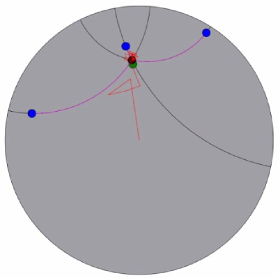
Figure 2: Median of three points in the Poicaré disc

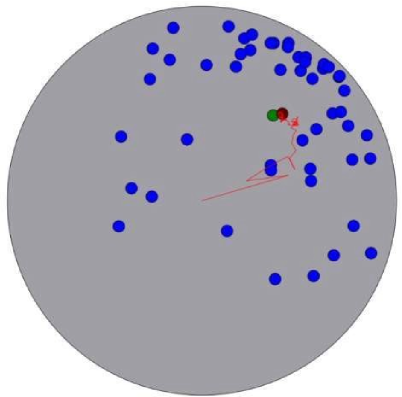
Figure 3: Median of points in the Poicaré disc

5.3 Computing $p$-means by gradient descent

Gradient descent algorithms for computing $e_{p}$ are given in the following theorem. In view of Theorem 3.4, it suffices to consider the case when $p>1$.

Theorem 5.3

Assume that $p>1$. Let $x_{0}\in\bar{B}(a,r)$ and for $k\geq 0$ define

$$x_{k+1}=\exp_{x_{k}}(-t_{k}\mathop{\rm grad}\nolimits_{x_{k}}H_{p}),$$

where $(t_{k})_{k}$ is a sequence of real numbers such that

$$0<t_{k}\leq\frac{p\varepsilon^{p+1}}{\pi p^{2}(2r)^{2p-1}\beta\coth(2\beta r)+p\varepsilon^{p}},\quad\lim_{k\rightarrow\infty}t_{k}=0\quad\text{and}\quad\sum_{k=0}^{\infty}t_{k}=+\infty.$$

Then the sequence $(x_{k})_{k}$ is contained in $\bar{B}(a,\rho)$ and converges to $e_{p}$.

The following proposition gives the error estimations of the gradient descent algorithms in Theorem 5.3.

Proposition 4

Assume that $t_{k}<C_{p,\mu,K}^{-1}$ for every $k$ in Theorem 5.3, then the following error estimations hold:
i) if $1<p<2$, then for $k\geq 1$,

$$\rho^{2}(x_{k},e_{p})\leq\mskip 3.0mu 4r^{2}\prod_{i=0}^{k-1}(1-C_{p,\mu,K}t_{i})$$

$$+C(\beta,r,p)\bigg{(}\sum_{j=1}^{k-1}t_{j-1}^{2}\prod_{i=j}^{k-1}(1-C_{p,\mu,K}t_{i})+t_{k-1}^{2}\bigg{)}:=b_{k};$$

ii) if $p\geq 2$, then for $k\geq 1$,

$$H_{p}(x_{k})-H_{p}(e_{p})\leq\mskip 3.0mu (2r)^{p}\prod_{i=0}^{k-1}(1-C_{p,\mu,K}t_{i})$$

$$+C(\beta,r,p)\bigg{(}\sum_{j=1}^{k-1}t_{j-1}^{2}\prod_{i=j}^{k-1}(1-C_{p,\mu,K}t_{i})+t_{k-1}^{2}\bigg{)}:=c_{k},$$

where the constant

$$C(\beta,r,p)=\begin{cases}p^{2}(2r)^{2p-1}\beta\coth(2\beta r),\mskip 3.0mu\mskip 3.0mu&\text{if \thinspace\thinspace$1<p<2$;}\\ p^{3}(2r)^{3p-4}\left(2\beta r\coth(2\beta r)+p-2\right),\mskip 3.0mu\mskip 3.0mu&\text{if \thinspace\thinspace$p\geq 2$.}\end{cases}$$

Moreover, the sequences $(b_{k})_{k}$ and $(c_{k})_{k}$ both tend to zero.

6 Riemannian geometry of Toeplitz covariance matrices
and applications to radar target detection

In this section we study the Riemannian geometry of the manifold of Toeplitz covariance matrices of order $n$. The explicit expression of the reflection coefficients reparametrization and its inverse are obtained. With the Riemannian metric given by the Hessian of a Kähler potential, we show that the manifold is in fact a Cartan-Hadamard manifold with lower sectional curvature bound $-4$. The geodesics in this manifold are also computed. Finally, we apply the subgradient algorithm introduced in section 3 and the Riemannian geometry of Toeplitz covariance matrices to radar target detection. We refer to [33] for more mathematical details of this section.

6.1 Reflection coefficients parametrization

Let $\mathcal{T}_{n}$ be the set of Toeplitz Hermitian positive definite matrices of order $n$. It is an open submanifold of $\mathbf{R}^{2n-1}$. Each element $R_{n}\in\mathcal{T}_{n}$ can be written as

$$R_{n}=\left[\begin{matrix}r_{0}&\overline{r}_{1}&\ldots&\overline{r}_{n-1}\\ r_{1}&r_{0}&\ldots&\overline{r}_{n-2}\\ \vdots&\ddots&\ddots&\vdots\\ r_{n-1}&\ldots&r_{1}&r_{0}\par\end{matrix}\right]\mskip 3.0mu.$$

For every $1\leq k\leq n-1$, the upper left $(k+1)$-by-$(k+1)$ corner of $R_{n}$ is denoted by $R_{k}$. It is associated to a $k$-th order autoregressive model whose Yule-Walker equation is

$$\left[\begin{matrix}r_{0}&\overline{r}_{1}&\ldots&\overline{r}_{k}\\ r_{1}&r_{0}&\ldots&\overline{r}_{k-1}\\ \vdots&\ddots&\ddots&\vdots\\ r_{k}&\ldots&r_{1}&r_{0}\par\end{matrix}\right]\left[\begin{matrix}1\\ a_{1}^{(k)}\\ \vdots\\ a_{k}^{(k)}\end{matrix}\right]=\left[\begin{matrix}P_{k}\\ 0\\ \vdots\\ 0\end{matrix}\right]\mskip 3.0mu,$$

where $a_{1}^{(k)},\dots,a_{k}^{(k)}$ are the optimal prediction coefficients and $P_{k}=\det R_{k+1}/\det R_{k}$ is the mean squared error.

The last optimal prediction coefficient $a_{k}^{(k)}$ is called the $k$-th reflection coefficient and is denoted by $\mu_{k}$. It is easily seen that $\mu_{1},\dots,\mu_{n-1}$ are uniquely determined by the matrix $R_{n}$. Moreover, the classical Levinson’s recursion gives that $|\mu_{k}|<1$. Hence, by letting $P_{0}=r_{0}$, we obtain a map between two submanifolds of $\mathbf{R}^{2n-1}$:

$$\varphi:\quad\mathcal{T}_{n}\longrightarrow\mathbf{R}^{*}_{+}\times\mathbf{D}^{n-1},\quad R_{n}\longmapsto(P_{0},\mu_{1},\dots,\mu_{n-1}),$$

where $\mathbf{D}=\{z\in\mathbf{C}:|z|<1\}$ is the unit disc of the complex plane.

Using the Cramer’s rule and the method of Schur complement we get the following proposition.

Proposition 5

$\varphi$ is a diffeomorphism, whose explicit expression is

$$\mu_{k}=(-1)^{k}\frac{\det S_{k}}{\det R_{k}},\quad\text{where}\quad S_{k}=R_{k+1}\binom{2,\dots,k+1}{1,\dots,k}$$

is the submatrix of $R_{k+1}$ obtained by deleting the first row and the last column. On the other hand, if $(P_{0},\mu_{1},\dots,\mu_{n-1})\in\mathbf{R}^{*}_{+}\times\mathbf{D}^{n-1}$, then its inverse image $R_{n}$ under $\varphi$ can be calculated by the following algorithm:

$$r_{0}=P_{0},\quad r_{1}=-P_{0}\mu_{1},$$

$$r_{k}=-\mu_{k}P_{k-1}+\alpha^{T}_{k-1}J_{k-1}R_{k-1}^{-1}\alpha_{k-1},\quad 2\leq k\leq n-1,$$

where

$$\alpha_{k-1}=\left[\begin{matrix}r_{1}\\ \vdots\\ r_{k-1}\end{matrix}\right],\quad J_{k-1}=\left[\begin{matrix}0&\ldots&0&1\\ 0&\ldots&1&0\\ &\ldots\\ 1&\ldots&0&0\end{matrix}\right]\quad\text{and}\quad P_{k-1}=P_{0}\prod_{i=1}^{k-1}(1-|\mu_{i}|^{2}).$$

6.2 Riemannian geometry of Toeplitz covariance matrices

From now on, we regard $\mathcal{T}_{n}$ as a Riemannian manifold whose metric, which is introduced in [8] by the Hessian of the Kähler potential

$$\Phi(R_{n})=-\ln(\det R_{n})-n\ln(\pi e),$$

is given by

$$ds^{2}=n\frac{dP_{0}^{2}}{P_{0}^{2}}+\sum_{k=1}^{n-1}(n-k)\frac{|d\mu_{k}|^{2}}{(1-|\mu_{k}|^{2})^{2}},$$ (8)

where $(P_{0},\mu_{1},\dots,\mu_{n-1})=\varphi(R_{n})$.

The metric (8) is a Bergman type metric and it has be shown in [33] that this metric is not equal to the Fisher information metric of $\mathcal{T}_{n}$. But J. Burbea and C. R. Rao have proved in [18, Theorem 2] that the Bergman metric and the Fisher information metric do coincide for some probability density functions of particular forms. A similar potential function was used by S. Amari in [2] to derive the Riemannian metric of multi-variate Gaussian distributions by means of divergence functions. We refer to [29] for more account on the geometry of Hessian structures.

With the metric given by (8) the space $\mathbf{R}^{*}_{+}\times\mathbf{D}^{n-1}$ is just the product of the Riemannian manifolds $(\mathbf{R}^{*}_{+},ds^{2}_{0})$ and $(\mathbf{D},ds^{2}_{k})_{1\leq k\leq n-1}$, where

$$ds_{0}^{2}=n\frac{dP^{2}_{0}}{P_{0}^{2}}\quad\text{and}\quad ds^{2}_{k}=(n-k)\frac{|d\mu_{k}|^{2}}{(1-|\mu_{k}|^{2})^{2}}.$$

The latter is just $n-k$ times the classical Poincaré metric of $\mathbf{D}$. Hence $(\mathbf{R}^{*}_{+}\times\mathbf{D}^{n-1},ds^{2})$ is a Cartan-Hadamard manifold whose sectional curvatures $K$ verify $-4\leq K\leq 0$. The Riemannian distance between two different points $x$ and $y$ in $\mathbf{R_{+}^{*}}\times\mathbf{D}^{n-1}$ is given by

$$d(x,y)=\bigg{(}n\sigma(P,Q)^{2}+\sum_{k=1}^{n-1}(n-k)\tau(\mu_{k},\nu_{k})^{2}\bigg{)}^{1/2},$$

where $x=(P,\mu_{1},\ldots,\mu_{n-1})$, $y=(Q,\nu_{1},\ldots,\nu_{n-1})$,

$$\sigma(P,Q)=|\ln(\frac{Q}{P})|\quad\text{and}\quad\tau(\mu_{k},\nu_{k})=\frac{1}{2}\ln\frac{1+|\frac{\nu_{k}-\mu_{k}}{1-\bar{\mu}_{k}\nu_{k}}|}{1-|\frac{\nu_{k}-\mu_{k}}{1-\bar{\mu}_{k}\nu_{k}}|}.$$

The geodesic from $x$ to $y$ in $\mathcal{T}_{n}$ parameterized by arc length is given by

$$\gamma(s,x,y)=(\gamma_{0}(\frac{\sigma(P,Q)}{d(x,y)}s),\gamma_{1}(\frac{\tau(\mu_{1},\nu_{1})}{d(x,y)}s),\ldots,\gamma_{1}(\frac{\tau(\mu_{n-1},\nu_{n-1})}{d(x,y)}s)),$$

where $\gamma_{0}$ is the geodesic in $(\mathbf{R_{+}^{*}},ds^{2}_{0})$ from $P$ to $Q$ parameterized by arc length and for $1\leq k\leq n-1$, $\gamma_{k}$ is the geodesic in $(\mathbf{D},ds^{2}_{k})$ from $\mu_{k}$ to $\nu_{k}$ parameterized by arc length. More precisely,

$$\gamma_{0}(t)=Pe^{t\mathop{\rm sign}\nolimits(Q-P)},$$

and for $1\leq k\leq n-1$,

$$\gamma_{k}(t)=\frac{(\mu_{k}+e^{i\theta_{k}})e^{2t}+(\mu_{k}-e^{i\theta_{k}})}{(1+\bar{\mu}_{k}e^{i\theta_{k}})e^{2t}+(1-\bar{\mu}_{k}e^{i\theta_{k}})},\quad\text{where}\quad\theta_{k}=\arg\frac{\nu_{k}-\mu_{k}}{1-\bar{\mu}_{k}\nu_{k}}.$$

Particularly,

$$\gamma^{\prime}(0,x,y)=(\gamma_{0}^{\prime}(0)\frac{\sigma(P,Q)}{d(x,y)},\gamma_{1}^{\prime}(0)\frac{\tau(\mu_{1},\nu_{1})}{d(x,y)},\ldots,\gamma_{n-1}^{\prime}(0)\frac{\tau(\mu_{n-1},\nu_{n-1})}{d(x,y)}).$$

Let $v=(v_{0},v_{1},\ldots,v_{n-1})$ be a tangent vector in $T_{x}(\mathbf{R}_{+}^{*}\times\mathbf{D}^{n-1})$, then the geodesic starting from $x$ with velocity $v$ is given by

$$\zeta(t,x,v)=(\zeta_{0}(t),\zeta_{1}(t),\ldots,\zeta_{n-1}(t)),$$

where $\zeta_{0}$ is the geodesic in $(\mathbf{R}_{+}^{*},ds^{2}_{0})$ starting from $P$ with velocity $v_{0}$ and for $1\leq k\leq n-1$, $\zeta_{k}$ is the geodesic in $(\mathbf{D},ds^{2}_{k})$ starting from $\mu_{k}$ with velocity $v_{k}$. More precisely,

$$\zeta_{0}(t)=Pe^{\frac{v_{0}}{P}t},$$

and for $1\leq k\leq n-1$,

$$\zeta_{k}(t)=\frac{(\mu_{k}+e^{i\theta_{k}})e^{\frac{2|v_{k}|t}{1-|\mu_{k}|^{2}}}+(\mu_{k}-e^{i\theta_{k}})}{(1+\bar{\mu}_{k}e^{i\theta_{k}})e^{\frac{2|v_{k}|t}{1-|\mu_{k}|^{2}}}+(1-\bar{\mu}_{k}e^{i\theta_{k}})},\quad\text{where}\quad\theta_{k}=\arg v_{k}.$$

6.3 Radar simulations

Now we give some simulating examples of the median method applied to radar target detection.

Since the autoregressive spectra are closely related to the speed of targets, we shall first investigate the spectral performance of the median method. In order to illustrate the basic idea, we only consider the detection of one fixed direction. The range along this direction is subdivided into 200 lattices in which we add two targets, the echo of each lattice is modeled by an autoregressive process. The following Figure 4 gives the initial spectra of the simulation, where $x$ axis represents the lattices and $y$ axis represents frequencies. Every lattice is identified with a $1\times 8$ vector of reflection coefficients which is calculated by using the regularized Burg algorithm [11] to the original simulating data. The spectra are represented by different colors whose corresponding values are indicated in the colorimetric on the right.

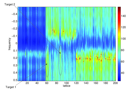
Figure 4: Initial spectra with two added targets

For every lattice, by using the subgradient algorithm, we calculate the median of the window centered on it and consisting of 15 lattices and then we get the spectra of medians shown in Figure 6. Furthermore, by comparing it with Figure 6 which are spectra of barycenters, we see that in the middle of the barycenter spectra, this is just the place where the second target appears, there is an obvious distortion. This explains that median is much more robust than barycenter when outliers come.

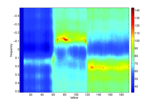
Figure 5: Median spectra

Figure 6: Barycenter spectra

The principle of target detection is that a target appears in a lattice if the distance between this lattice and the median of the window around it is much bigger than that of the ambient lattices. The following Figure 7 shows that the two added targets are well detected by the median method, where $x$ axis represents lattice and $y$ axis represents the distance in $\mathcal{T}_{8}$ between each lattice and the median of the window around it.

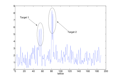
Figure 7: Detection by median

We conclude our discussion by showing the performance of the median method in real target detection. As above, we give the images of autoregressive spectra and the figure of target detection obtained by using real data which are records of a radar located on a coast. These records consist of about 5000 lattices of a range of about 10km-140km as well as 109 azimuth values corresponding to approximately 30 scanning degrees of the radar. For simplicity we consider the data of all the lattices but in a fixed direction, hence each lattice corresponds to a $1\times 8$ vector of reflection coefficients computed by applying the regularized Burg algorithm to the original real data. Figure 9 gives the initial autoregressive spectra whose values are represented by different color according to the colorimetric on the right. For each lattice, by using the subgradient algorithm, we calculate the median of the window centered on it and consisting of 17 lattices and then we get the spectra of medians shown in Figure 9.

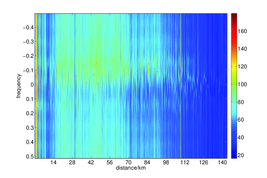
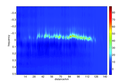
Figure 8: Initial spectra of real radar data

Figure 9: Median spectra of real radar data

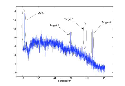
Figure 10: Real detection by median

In order to know in which lattice target appears, we compare the distance between each lattice and the median of the window around it. The following Figure 10 shows that the four targets are well detected by our method, where $x$ axis represents distance and $y$ axis represents the distance in $\mathcal{T}_{8}$ between each lattice and the median of the window around it.

References

- [1] B. Afsari, Riemannian center of mass : existence, uniqueness, and convexity, Proceedings of the American Mathematical Society, S 0002-9939(2010)10541-5, Article electronically published on August 27, 2010.
- [2] S. Amari and A. Cichocki, Information geometry of divergence functions, Bulletin of the Polish Academy of Sciences, Technical Sciences, Vol. 58, No. 1, 2010.
- [3] M. Arnaudon and X. M. Li, Barycenters of measures transported by stochastic flows, The Annals of probability, 33 (2005), no. 4, 1509-1543.
- [4] M. Arnaudon, C. Dombry, A. Phan and L. Yang, Stochastic algorithms for computing means of probability measures, preprint hal-00540623, version 2, (2011). to appear in Stochastic Processes and their Applications.
- [5] M. Arnaudon and F. Nielsen, On approximating the Riemannian 1-center, hal-00560187-version 1 (2011).
- [6] M. Arnaudon and F. Nielsen, Medians and means in Finsler geometry, hal-00540625-version 2 (2011), to appear in LMS J. Comput. Math.
- [7] F. Barbaresco, Innovative Tools for Radar Signal Processing Based on Cartan’s Geometry of SPD Matrices and Information Geometry, IEEE International Radar Conference (2008).
- [8] F. Barbaresco, Interactions between Symmetric Cone and Information Geometries, ETVC’08, Springer Lecture Notes in Computer Science 5416 (2009), pp. 124-163.
- [9] F. Barbaresco and G. Bouyt, Espace Riemannien symétrique et géométrie des espaces de matrices de covariance : équations de diffusion et calculs de médianes, GRETSI’09 conference, Dijon, September 2009
- [10] F. Barbaresco, New Foundation of Radar Doppler Signal Processing based on Advanced Differential Geometry of Symmetric Spaces: Doppler Matrix CFAR and Radar Application, Radar’09 Conference, Bordeaux, October 2009
- [11] F. Barbaresco, Annalyse Doppler: régularisation d’un problème inverse mal posé, Support de cours
- [12] F. Barbaresco, Science géométrique de l Information : Géométrie des matrices de covariance, espace métrique de Fréchet et domaines bornés homogénes de Siegel, Conférence GRETSI’11, Bordeaux, Sept. 2011
- [13] F. Barbaresco, Robust Statistical Radar Processing in Fréchet Metric Space: OS-HDR-CFAR and OS-STAP Processing in Siegel Homogeneous Bounded Domains, Proceedings of IRS’11, International Radar Conference, Leipzig, Sept. 2011
- [14] F. Barbaresco, Geometric Radar Processing based on Fréchet Distance : Information Geometry versus Optimal Transport Theory, Proceedings of IRS’11, International Radar Conference, Leipzig, Sept. 2011
- [15] R. Bhattacharya and V. Patrangenaru, Large sample theory of intrinsic and extrinsic sample means on manifolds. I, The Annals of Statistics, 2003, Vol 31, No. 1, 1-29
- [16] M. Bridson and A. Haefliger, Metric spaces of non-positive curvature, (Springer, Berlin, 1999).
- [17] S. R. Buss and J. P. Fillmore, Spherical averages and applications to spherical splines and interpolation, ACM Transactions on Graphics vol. 20(2001), pp. 95-126.
- [18] J. Burbea and C. R. Rao, Differntial metrics in probability spaces, Probability and Mathematical Statistics, Vol. 3, Fasc. 2, pp. 241-258, 1984.
- [19] Z. Drezner and G. O. Wesolowsky, Facility location on a sphere, J. Opl Res Soc. Vol. 29, 10, pp. 997-1004.
- [20] Z. Drezner, On location dominance on spherical surfaces, Operation Research, Vol. 29, No. 6, November-December 1981, pp. 1218-1219.
- [21] M. Emery and G. Mokobodzki, Sur le barycentre d’une probabilité dans une variété, Séminaire de Probabilités-XXV, Lecture Notes in Mathematics 1485. (Springer, Berlin, 1991), pp. 220-233.
- [22] P. T. Fletcher et al., The geometric median on Riemannian manifolds with application to robust atlas estimation, NeuroImage, 45 (2009), S143-S152.
- [23] M. Fréchet, Les éléments aléatoires de natures quelconque dans un espace distancié, Annales de l’I.H.P., tome 10, no4 (1948), p. 215-310.
- [24] H. Karcher, Riemannian center of mass and mollifier smoothing, Communications on Pure and Applied Mathematics, vol xxx (1977), 509-541.
- [25] W. S. Kendall, Probability, convexity, and harmonic maps with small image I: uniqueness and fine existence, Proc. London Math. Soc., (3) 61 (1990), no. 2, 371-406.
- [26] R. Noda, T. Sakai and M. Morimoto, Generalized Fermat’s problem, Canad. Math. Bull. Vol. 34(1), 1991, pp. 96-104.
- [27] J. Picard, Barycentres et martingales sur une variété, Ann. Inst. H. Poincaré Probab. Statist, 30 (1994), no. 4, 647-702.
- [28] A. Sahib, Espérance d’une variable aléatoire à valeur dans un espace métrique, Thèse de l’Université de Rouen (1998).
- [29] H. Shima, The geometry of hessian structures, World Scientific Publishing (2007).
- [30] C. Villani, Optimal Transport: Old and New. Springer-Verlag, 2009.
- [31] L. Yang, Riemannian median and its estimation, LMS J. Comput. Math. vol 13 (2010), pp. 461-479.
- [32] L. Yang, Some properties of Fréchet medians in Riemannian manifolds, preprint (2011), submitted.
- [33] L. Yang, Médianes de mesures de probabilité dans les variétés riemanniennes et applications à la détection de cibles radar, Thèse de l’Université de Poitiers, 2011.