Model Checking Probabilistic Real-Time Properties for Service-Oriented Systems with Service Level Agreements

Abstract

The assurance of quality of service properties is an important aspect of service-oriented software engineering. Notations for so-called service level agreements (SLAs), such as the Web Service Level Agreement (WSLA) language, provide a formal syntax to specify such assurances in terms of (legally binding) contracts between a service provider and a customer. On the other hand, formal methods for verification of probabilistic real-time behavior have reached a level of expressiveness and efficiency which allows to apply them in real-world scenarios. In this paper, we suggest to employ the recently introduced model of Interval Probabilistic Timed Automata (IPTA) for formal verification of QoS properties of service-oriented systems. Specifically, we show that IPTA in contrast to Probabilistic Timed Automata (PTA) are able to capture the guarantees specified in SLAs directly. A particular challenge in the analysis of IPTA is the fact that their naive semantics usually yields an infinite set of states and infinitely-branching transitions. However, using symbolic representations, IPTA can be analyzed rather efficiently. We have developed the first implementation of an IPTA model checker by extending the PRISM tool and show that model checking IPTA is only slightly more expensive than model checking comparable PTA.

1 Introduction

One of the key tasks in engineering service-oriented systems is the assurance of quality of service (QoS) properties, such as ‘the response time of a service is less than 20ms for at least $95\%$ of the requests’. Service level agreements (SLAs) provide a notation for specifying such guarantees in terms of (legally binding) contracts between a service provider and a service consumer. A specific example for an SLA notation is the Web Service Level Agreement (WSLA) [9, 4] language, which provides a formal syntax to specify such QoS guarantees for web services. The compliance of a service implementation with an SLA is commonly checked at runtime by means of monitoring them.

However, due to the fact that an application or service may itself make use of other services, guaranteeing probabilistic real-time properties can be difficult. The problem becomes even harder, when the service is not bound to a specific service provider but linked dynamically. Statistical testing of the service consumer together with all currently possible service providers can provide some evidence that the required probabilistic real-time properties hold. However, each time a new service provider is connected or in situations when a known service provider slightly changes the characteristics of the offered service, the test results are no longer representative.

In the last couple of years, formal methods for verification of probabilistic real-time behavior have reached a level of expressiveness and efficiency that allows to apply them to real-world case studies in various application domains, including communication and multimedia protocols, randomized distributed algorithms and biological systems (cf. [16, 18]). Therefore, it is a natural step to investigate also their suitability to address the outlined challenges for guaranteeing QoS properties of service-oriented systems. In particular, dynamically linking of services in service-oriented systems introduces major difficulties concerning the analysis of their QoS properties.

In this paper, we suggest to employ the recently introduced model of Interval Probabilistic Timed Automata [19] (IPTA) which extend Probabilistic Timed Automata [13] (PTA) by permitting to specify intervals, i.e., lower and upper bounds for probabilities, rather than exact values. The contributions of this paper can be summarized as follows: (1) We show that IPTA (in contrast to PTA) are able to capture the guarantees specified in SLAs directly. The notion of probabilistic uncertainty in IPTA allows modeling and verifying service-oriented systems with dynamic service binding, where one can rely only on the guarantees stated in the SLA and no knowledge about the actual service implementation is available. (2) To the best of our knowledge, we present the first implementation of an IPTA model checker and show that it can analyze IPTA nearly as fast as comparable PTA. (3) We show that a naive analysis using sampling of PTA does not yield the correct results as predicted by IPTA. Furthermore, we provide evidence that checking equivalent PTA has a worse performance than checking the IPTA directly.

Organization

The rest of this paper is organized as follows. Section 2 demonstrates that IPTA naturally permit to capture the guarantees of an SLA when modeling the behavior of a service provider. Section 3 introduces the syntax and semantics of interval probabilistic timed automata. Section 4 discusses symbolic PTCTL model checking and the probabilistic reachability problem. In Section 5 we present our tool support. In Section 6 we show that IPTA checking is only slightly more expensive than PTA checking. We show that using sampling of the probability values in the intervals to derive a representative set of PTA does neither scale as good as IPTA checking nor does it work correctly. Finally, we demonstrate that also an encoding of IPTA in form of a PTA does not scale as good as IPTA checking. In Section 7 we discuss related work. Section 8 contains conclusions and future work.

2 Quality of Service Modeling

Since in the service-oriented paradigm, compositionality is employed to construct new services and applications, the interaction behavior of a service-oriented system can be captured by a set of communicating finite state automata. For instance, a simple service-oriented system can consist of a service provider and a service consumer, both represented as automata, which communicate according to a specific protocol, given by a service contract.

The QoS of a service-oriented application is often as important as its functional properties. Validation of QoS characteristics usually requires models, which capture probabilistic aspects as well as real-time properties. Probabilistic Timed Automata [13] (PTA) are an expressive, compositional model for probabilistic real-time behavior with support for non-determinism. However, a limitation of PTA is the fact that only fixed values for probabilities can be expressed. In practice, it is often only possible to approximate probabilities with guarantees for lower and upper bounds. For this reason, Interval Probabilistic Timed Automata [19] (IPTA) generalize PTA by allowing to specify intervals of probabilities as opposed to fixed values. This feature is particularly useful to model guarantees for probabilities as commonly found in service level agreements (SLAs).

Listing 1: A response time guarantee in WSLA

⬇

1<Metric name="NormalResponsePercentage" type="float" unit="Percentage">

2 <Source>ServiceProvider</Source>

3 <Function resultType="float" xsi:type="wsla:PercentageLessThanThreshold">

4 <Metric>ResponseTime</Metric>

5 <Value>

6 <LongScalar>20</LongScalar> <!-- Normal responses take less than 20ms -->

7 </Value>

8 </Function>

9</Metric>

10

11<Obligations>

12 <ServiceLevelObjective name="ResponseTimeGuarantee">

13 <Obliged>ServiceProvider</Obliged>

14 <Expression>

15 <Predicate xsi:type="GreaterEqual">

16 <SLAParameter>NormalResponsePercentage</SLAParameter>

17 <Value>0.95</Value> <!-- At least 95% normal responses -->

18 </Predicate>

19 </Expression>

20 </ServiceLevelObjective>

21<Obligations>

As a concrete example of an SLA, Listing 1 contains an adaption of a WSLA specification presented in [9]. In the upper part, a metric called NormalResponsePercentage is defined which contains the percentage of response events which took less than 20ms. The actual service level agreement is defined in the lower part in terms of a service provider obligation called ResponseTimeGuarantee. This obligation assures that the percentage of responses that take less than 20ms is at least $95\%$.

Figure 1 depicts a PTA for a client/server application in which the server guarantees a probability of (exactly) 95% for response times of less than 20ms. The client is modeled as another PTA which synchronizes with the server using the request and response actions. Note that the client model is actually just a Timed Automata (TA), because no probabilities are employed. However, in the cases where probabilities also matter, we would need exact knowledge of them to be able construct a proper PTA.

Figure 1: PTA for a client (left) and a server (right)

This small example shows that PTA, similarly to other automata models, consist of set of states (or locations) and transitions (or edges). The time related behavior is specified using clocks (as $x$ in the server) which can be reset ($x:=0$), tested in conditions for transitions ($x\geq 20$) and also state invariants ($x<20$ for $s_{2}$). Note that we use the constant $T$ to denote a constant timeout value in the invariant $x<T$. A clock such as $x$ simply increases with progressing time, unless it is explicitly reset. The conditions block the transition until the clock constraint is fulfilled. Moreover, the state invariant ensures that (1) no transition leads to this state when this would result in invalidating the state invariant, and (2) the automaton can no longer stay in this state when this would also lead to a violation of the invariant. In addition to purely non-deterministic behavior, i.e. when multiple transitions with the same action are enabled, probabilities can be associated with transitions, e.g. $0.95$ for the request transition leading to the state $s_{2}$, and $0.05$ leading to the state $s_{3}$. Note that for probabilistic transitions, all alternative branches must sum up to $1$. Formally, the target of a transition in a PTA is not a single state, but a discrete probability distribution over the set of all states. Thus, in addition to purely nondeterministic choice, PTA allow to specify the likelihood of an event. Note also that the existence of a parallel operator (written as $\mathcal{P}_{1}\parallel\mathcal{P}_{2}$ where $\mathcal{P}_{1}$ and $\mathcal{P}_{2}$ are PTA) moreover allows to synchronize two automata via shared actions, which enables compositional modeling.

However, the Interval Probabilistic Timed Automaton (IPTA) of a server in Figure 2 additionally allows to capture the ‘at least $95\%$’ semantics of the SLA in Listing 1. The difference to the PTA model is that in IPTA it is possible to specify probabilistic behavior with a level of uncertainty. Specifically, IPTA allow to specify intervals of probabilisties as opposed to the exact probabilities used in PTA. The semantics of intervals in contrast to exact values is that each time a probabilistic decision is necessary, any of the usually uncountable many probability distributions which lie within the lower and upper bounds of the intervals denote a valid behavior. Therefore, probability intervals match better with the guarantees commonly found in SLAs, such as ‘with at least 95% a request is answered within 20ms’. Note that we did not model the client as another IPTA here, but just as the TA in Figure 1. However, similarly to the modeled server, we can also model uncertain probabilistic behavior in the client, such as ‘with at least 75% a request is made within 50ms’. The parallel composition of IPTA then allows to derive a model of the complete system.

Figure 2: IPTA for a simple server

Given such models in form of PTA or IPTA, we can now employ model checking to verify probabilistic real-time properties for the composed system, specified in an appropriate probabilistic real-time logic. In our case, we might be interested in the property ‘the probability that 1 out of 10 responses is too slow is at most 5%’. As we will demonstrate later in this paper, there are important differences between the outcome of such an analysis depending on whether we employ the PTA using exact probabilities or the IPTA which allows to specify only lower and upper bounds. In particular, no sample set of PTA derived from the IPTA by choosing values from the interval is in general sufficient to derive the same result as the analysis of the IPTA.

3 Interval Probabilistic Timed Automata

Interval probabilistic timed automata (IPTA) [19] integrate the probabilistic real-time modeling concepts of probabilistic timed automata (PTA) [13] and the idea of probabilistic uncertainty known from interval Markov chains [17]. Thus, they not only provide a way to distinguish between purely probabilistic and nondeterministic (timed) behavior, but also allow to specify uncertain probabilities using lower and upper bounds. These ingredients make IPTA a suitable formal model for the specification and verification of QoS assurances that can be commonly found in SLAs.

3.1 Preliminaries

Discrete probability distributions

For a finite set $S$, $\mathit{Dist}(S)$ is the set of discrete probability distributions over $S$, i.e., the set of all functions $\mu:S\to[0,1]$, with $\sum_{s\in S}\mu(s)=1$. The point distribution $\mu_{s}^{\bullet}$ is the unique distribution on $S$ with $\mu(s)=1$.

Clocks, valuations and constraints

Let $\mathbb{R}_{+}$ denote the set of non-negative reals. Let $\mathcal{X}=\{x_{1},\ldots,x_{n}\}$ be a set of variables in $\mathbb{R}_{+}$, called clocks. An $\mathcal{X}$-valuation is a map $v:\mathcal{X}\to\mathbb{R}_{+}$. For a subset $X\subseteq\mathcal{X}$, $v[X:=0]$ denotes the valuation $v^{\prime}$ with $v^{\prime}(x)=0$ if $x\in X$ and $v^{\prime}(x)=v(x)$ if $x\notin X$. For $d\in\mathbb{R}_{+}$, $v+d$ is the valuation $v^{\prime\prime}$ with $v^{\prime\prime}(x)=v(x)+d$ for all $x\in\mathcal{X}$. A clock constraint $\zeta$ on $\mathcal{X}$ is an expression of the form $x\bowtie c$ or $x-y\bowtie c$ such that $x,y\in\mathcal{X}$, $c\in\mathbb{R}_{+}$ and $\bowtie\;\in\{\leq,<,>,\geq\}$, or a conjunction of clock constraints. A clock valuation $v$ satisfies $\zeta$, written as $v\triangleright\zeta$ if and only if $\zeta$ evaluates to $\mathrm{true}$ when all clocks $x\in\mathcal{X}$ are substituted with their clock value $v(x)$. Let $\mathit{CC}(\mathcal{X})$ denote the set of all clock constraints over $\mathcal{X}$.

3.2 Syntax

Before defining IPTA formally, we introduce a syntactical and, thus, finite notion of probability interval distributions.

Definition 3.1 (Interval distribution)

Let $S$ be a finite set. A probability interval distribution $\lambda$ on $S$ is a pair of functions $\lambda=\langle\lambda^{\ell},\lambda^{u}\rangle$ with $\lambda^{\ell},\lambda^{u}:S\to[0,1]$, such that $\lambda^{\ell}(s)\leq\lambda^{u}(s)$ for all $s\in S$ and furthermore:

$$\sum_{s\in S}\lambda^{\ell}(s)\leq 1\leq\sum_{s\in S}\lambda^{u}(s)$$ (1)

The set of probability interval distributions over $S$ is denoted by $\mathit{IntDist}(S)$. The support of $\lambda$ is defined as $\mathit{Supp}(\lambda)=\{s\in S\;|\;\lambda^{u}(s)>0\}$. Let $\lambda^{\bullet}_{s}$ be the unique interval distribution that assigns $\langle 1,1\rangle$ to $s$, and $\langle 0,0\rangle$ to all $t\in S,t\neq s$.

A probability interval distribution $\lambda$ is a symbolic representation of the non-empty, possibly infinite set of probability distributions that are conform with the interval bounds: $\{\,\mu\in\mathit{Dist}(S)\;|\;\forall s\in S:\lambda^{\ell}(s)\leq\mu(s)\leq\lambda^{u}(s)\,\}$. If clear from the context, we may abuse notation and identify $\lambda$ with this set and also write $\mu\in\lambda$ if and only if $\mu$ respects the bounds of $\lambda$. Note that interval distributions are also used (in a slightly different syntax) in the notion of closed interval specifications in [6]. However, the explicit definition using lower and upper interval bounds in our model enables a syntactical treatment of interval distributions which is useful, e.g., in the following notion of minimal interval distributions.

Definition 3.2 (Minimal interval distribution)

An interval distribution $\lambda$ on $S$ is called minimal if for all $s\in S$ the following conditions hold:

1. $\lambda^{u}(s)+\sum_{t\in S,t\neq s}\lambda^{\ell}(t)\leq 1$

2. $\lambda^{\ell}(s)+\sum_{t\in S,t\neq s}\lambda^{u}(t)\geq 1$

Minimal interval distributions have the property that the bounds of all intervals can be reached (but not necessarily at the same time). Although minimality is formally not needed in the properties that we consider here, it is often a desirable requirement since it can serve as a sanity check for a specification. For instance, the interval distribution $\lambda=\{\,s\mapsto\langle 0.4,0.5\rangle,t\mapsto\langle 0.4,0.5\rangle\,\}$ is not minimal because condition 2 is violated. Here, the lower bounds of $0.4$ can never be reached. In fact, the only probability distribution that is conform with the interval bounds is $\mu=\{\,s\mapsto 0.5,t\mapsto 0.5\,\}$. Thus, the minimality condition is a useful requirement which allows to verify the validity of interval bounds. Note also that it is always possible to derive a minimal interval distribution from a non-minimal one by pruning the interval bounds, e.g., by setting $\lambda^{u}(s):=1-\sum_{t\in S,t\neq s}\lambda^{\ell}(t)$ if condition 1 is violated for the state $s$.

Definition 3.3 (Interval probabilistic timed automaton)

An interval probabilistic timed automaton is a tuple $\mathcal{I}=(L,L^{0},\mathcal{A},\mathcal{X},\mathit{inv},\mathit{prob},\mathcal{L})$ consisting of:

• a finite set of locations $L$ with $L^{0}\subseteq L$ the set of initial locations,

• a finite set of action $\mathcal{A}$,

• a finite set of clocks $\mathcal{X}$,

• a clock invariant assignment function $\mathit{inv}:L\to\mathit{CC}(\mathcal{X})$

• a probabilistic edge relation $\mathit{prob}\;\subseteq L\times\mathit{CC}(\mathcal{X})\times\mathcal{A}\times\mathit{IntDist}(2^{\mathcal{X}}\times L)$, and

• a labeling function $\mathcal{L}:L\to 2^{\mathit{AP}}$ assigning atomic propositions to locations.

Note that for more flexibility and a clear separation between communication and state invariants, our IPTA model contains both actions on transitions and atomic propositions for states. This approach is also in line with our tool support based on an extended version of PRISM (see Section 5).

As an example, we consider the IPTA model of a simple server depicted in Figure 2, where we denote interval distributions by small black circles. The set of actions is $\mathcal{A}=\{\mathit{request},\mathit{response}\}$, and the clocks are $\mathcal{X}=\{x\}$. For simplicity, we do not include atomic propositions here. Moreover, we associate the interval $[1,1]$ with edges that have a support of size $1$. The server modeled by this IPTA responds to an incoming request within $20$ms with a probability between $95\%$ and $100\%$. These lower and upper bounds can arise in scenarios where the exact probabilities are unknown or cannot be given precisely, e.g., due to implementation details. For instance, one can imagine that the server relays all requests to an heterogeneous, internal server farm, in which the success probability depends on the currently chosen server.

Composition

An important aspect of the service-oriented paradigm is compositionality, i.e., the fact that new services can be built by composing existing ones. Therefore, it is also crucial to support composition at the modeling level. In our approach, a parallel operator for IPTA is used for this purpose. The parallel composition of IPTA is defined analogously to the one for PTA. However, we need to compose interval distributions instead of probability distributions.

Definition 3.4 (Parallel composition)

The parallel composition of two interval probabilistic timed automata $\mathcal{I}_{i}=(L_{i},L^{0}_{i},\mathcal{A}_{i},\mathcal{X}_{i},\mathit{inv}_{i},\mathit{prob}_{i},\mathcal{L}_{i})$ with $i\in\{1,2\}$ is defined as:

$$\mathcal{I}_{1}\parallel\mathcal{I}_{2}=(L_{1}\times L_{2},L^{0}_{1}\times L^{0}_{2},\mathcal{A}_{1}\cup\mathcal{A}_{2},\mathcal{X}_{1}\cup\mathcal{X}_{2},\mathit{inv},\mathit{prob},\mathcal{L})$$

such that

• $\mathcal{L}(\langle l_{1},l_{2}\rangle)=\mathcal{L}_{1}(l_{1})\cup\mathcal{L}_{2}(l_{2})$ for all $l_{1}\in L_{1},l_{2}\in L_{2}$

• $\mathit{inv}(\langle l_{1},l_{2}\rangle)=\mathit{inv}_{1}(l_{1})\wedge\mathit{inv}_{2}(l_{2})$ for all $l_{1}\in L_{1},l_{2}\in L_{2}$

• $\langle\langle l_{1},l_{2}\rangle,\zeta,a,\lambda\rangle\in\;\mathit{prob}$ if and only if one of the following conditions hold:

  1. $a\in\mathcal{A}_{1}\setminus\mathcal{A}_{2}$ and there exists $\langle l_{1},\zeta,a,\lambda_{1}\rangle\in\;\mathit{prob}_{1}$ such that $\lambda=\lambda_{1}\otimes\lambda^{\bullet}_{\langle\emptyset,l_{2}\rangle}$

  2. $a\in\mathcal{A}_{2}\setminus\mathcal{A}_{1}$ and there exists $\langle l_{2},\zeta,a,\lambda_{2}\rangle\in\;\mathit{prob}_{2}$ such that $\lambda=\lambda^{\bullet}_{\langle\emptyset,l_{1}\rangle}\otimes\lambda_{2}$

  3. $a\in\mathcal{A}_{1}\cap\mathcal{A}_{2}$ and there exists $\langle l_{i},\zeta_{i},a,\lambda_{i}\rangle\in\;\mathit{prob}_{i}$ such that $\lambda=\lambda_{1}\otimes\lambda_{2}$ and $\zeta=\zeta_{1}\wedge\zeta_{2}$

where for any $l_{i}\in L_{i}$, $X_{i}\subseteq\mathcal{X}_{i}$:

$$\lambda_{1}\otimes\lambda_{2}(X_{1}\cup X_{2},\langle l_{1},l_{2}\rangle)^{\ell} \overset{\mathrm{def}}{=}\lambda_{1}^{\ell}(X_{1},l_{1})\cdot\lambda_{2}^{\ell}(X_{2},l_{2})$$

$$\lambda_{1}\otimes\lambda_{2}(X_{1}\cup X_{2},\langle l_{1},l_{2}\rangle)^{u} \overset{\mathrm{def}}{=}\lambda_{1}^{u}(X_{1},l_{1})\cdot\lambda_{2}^{u}(X_{2},l_{2})$$

Thus, the product of two interval distributions is simply defined by the product of their lower and upper bounds. Note also that the parallel composition for IPTA synchronizes transitions via shared actions, and interleaves transitions via unshared actions.

3.3 Semantics

The semantics of IPTA can be given in terms of Timed Interval Probabilistic Systems (TIPS) [19], which are essentially infinite-state Interval Markov Decision Processes (IMDPs) [17].

Definition 3.5 (Timed interval probabilistic system)

A timed interval probabilistic system is a tuple $\mathcal{T}=(S,S^{0},\mathcal{A},\mathit{Steps},\mathcal{L})$ consisting of:

• a set of states $S$ with $S^{0}\subseteq S$ the set of initial states,

• a set of actions $\mathcal{A}$, such that $\mathcal{A}\cap\mathbb{R}_{+}=\emptyset$,

• a transition function $\mathit{Steps}:S\to 2^{(\mathcal{A}\cup\mathbb{R}_{+})\times\mathit{IntDist}(S)}$, such that, if $(a,\lambda)\in\mathit{Steps}(s)$ and $a\in\mathbb{R}_{+}$, then $\lambda$ is a point interval distribution, and

• a labeling function $\mathcal{L}:S\to 2^{\mathit{AP}}$ assigning atomic propositions to states.

The operational semantics of a timed interval probabilistic system can be understood as follows. A probabilistic transition, written as $s{\,\xrightarrow{a,\lambda,\mu}\,}s^{\prime}$, is made from a state $s\in S$ by:

1. nondeterministically selecting an action/duration and interval distribution pair $(a,\lambda)\in\mathit{Steps}(s)$,

2. nondeterministically choosing a probability distribution $\mu\in\lambda$,

3. making a probabilistic choice of target state $s^{\prime}$ according to $\mu$.

A path of a timed interval probabilistic system is a non-empty finite or infinite sequence of probabilistic transitions:

$$\omega=s_{0}\,\xrightarrow{a_{0},\lambda_{0},\mu_{0}}\,s_{1}\,\xrightarrow{a_{1},\lambda_{1},\mu_{1}}\,s_{2}\,\xrightarrow{a_{2},\lambda_{2},\mu_{2}}\,\ldots$$

where for all $i\in\mathbb{N}$ it holds that $s_{i}\in S$, $(a_{i},\lambda_{i})\in\mathit{Steps}(s_{i})$, $\mu_{i}\in\lambda_{i}$ and $\mu_{i}(s_{i})>0$. We denote with $\omega(i)$ the $(i+1)$th state of $\omega$, and with $\mathit{last}(\omega)$ the last state of $\omega$, if it is finite. An adversary is a particular resolution of the nondeterminism in a timed interval probabilistic system $\mathcal{T}$. Formally, an adversary $A$ for $\mathcal{T}$ is a function mapping every finite path $\omega$ of $\mathcal{T}$ to a triple $(a,\lambda,\mu)$, such that $(a,\lambda)\in\mathit{Steps}(\mathit{last}(\omega))$ and $\mu\in\lambda$. We restrict ourselves to time-divergent adversaries, i.e., we require that time has to advance beyond any given time bound. This is a common restriction in real-time models to rule out unrealizable behavior. The set of all time-divergent adversaries of $\mathcal{T}$ is denoted by $\mathit{Adv}_{\mathcal{T}}$.

For any $s\in S$ and adversary $A\in\mathit{Adv}_{\mathcal{T}}$, we let $\mathit{Paths}^{A}_{\mathit{finite}}(s)$ and $\mathit{Paths}^{A}_{\mathit{full}}(s)$ be the sets of all finite and infinite paths starting in $s$ that correspond to $A$, respectively. Under a given adversary, the behavior of a timed interval probabilistic system is purely probabilistic. Formally, an adversary for a timed interval probabilistic system induces an infinite discrete-time Markov chain and, thus, a probability measure $\mathit{Prob}^{A}_{s}$ over the set of paths $\mathit{Paths}^{A}_{\mathit{full}}(s)$ (cf. [10] for details). The semantics of an IPTA can be given by a TIPS as follows.

Definition 3.6 (TIPS semantics)

Given an IPTA $\mathcal{I}=(L,L^{0},\mathcal{A},\mathcal{X},\mathit{inv},\mathit{prob},\mathcal{L})$. The TIPS semantics of $\mathcal{I}$ is the timed interval probabilistic system $\mathcal{T}_{\mathcal{I}}=(S,S^{0},\mathcal{A},\mathit{Steps},\mathcal{L}^{\prime})$ where:

• $S\subseteq L\times\mathbb{R}_{+}^{\mathcal{X}}$, such that $\langle l,v\rangle\in S$ if and only if $v\triangleright\mathit{inv}(l)$,

• $S_{0}=\{\,\langle l,v[\mathcal{X}:=0]\rangle\;|\;l\in L^{0}\,\}$

• $\langle a,\lambda\rangle\in\mathit{Steps}(\langle l,v\rangle)$ if and only if one of the following conditions holds:

  • Time transitions: $a=t\in\mathbb{R}_{+}$, $\lambda=\lambda^{\bullet}_{\langle l,v+t\rangle}$ and $v+t^{\prime}\triangleright\mathit{inv}(l)$ for all $0\leq t^{\prime}\leq t$

  • Discrete transitions: $a\in\mathcal{A}$ and $\langle l,\zeta,\hat{\lambda}\rangle\in\mathit{prob}$ such that $v\triangleright\zeta$ and for any $\langle l^{\prime},v^{\prime}\rangle\in S$:

    • $\lambda^{\ell}(l^{\prime},v^{\prime})=\sum_{X\subseteq\mathcal{X}\wedge v^{\prime}=v[X:=0]}\hat{\lambda}^{\ell}(X,l^{\prime})$

    • $\lambda^{u}(l^{\prime},v^{\prime})=\sum_{X\subseteq\mathcal{X}\wedge v^{\prime}=v[X:=0]}\hat{\lambda}^{u}(X,l^{\prime})$

• $\mathcal{L}^{\prime}(\langle l,v\rangle)=\mathcal{L}(l)$ for all $\langle l,v\rangle\in S$.

4 Symbolic model checking

In this section, we recall the symbolic approach for PTCTL model checking as introduced for PTA in [14] and adapted for IPTA in [19]. Moreover, we discuss in more detail an iterative algorithm for computing the maximum and minimum probabilities for reaching a set of target states.

4.1 PTCTL – Probabilistic Timed Computation Tree Logic

Probabilistic Timed Computation Tree Logic (PTCTL) [13] can be used to specify combined probabilistic and timed properties. Constraints for probabilities in PTCTL are specified using the probabilistic threshold operator known from PCTL. Timing constraints in PTCTL are expressed using a set of system clocks $\mathcal{X}$, which are the clocks from the automaton to be checked, and a set of formula clocks $\mathcal{Z}$, which is disjoint from $\mathcal{X}$. The syntax of PTCTL is given by:

$$\phi::=a\;|\;\zeta\;|\;\neg\phi\;|\;\phi\vee\phi\;|\;z.\phi\;|\;\mathcal{P}_{\sim\kappa}[\phi\;\mathcal{U}\,\phi]$$

where:

• $a\in\mathit{AP}$ is an atomic proposition,

• $\zeta\in\mathit{CC}(\mathcal{X}\bigcup\mathcal{Z})$ is a clock constraint over all system and formula clocks,

• $z.\phi$ with $z\in\mathcal{Z}$ is a reset quantifier, and

• $\mathcal{P}_{\sim\kappa}[\_]$ is a probabilistic quantifier with $\sim\;\in\{\leq,<,>,$ $\geq\}$ and $\kappa\in[0,1]$ a probability threshold.

As an example for the specification of a combined probabilistic and timed property, the requirement for a bounded response time, e.g. ‘with a probability of at least 95% a response is sent within 20ms’ can be formalized in PTCTL as the formula:

$$z.\mathcal{P}_{\geq 0.95}[\mathrm{true}\;\mathcal{U}\,(\mathit{responseSent}\wedge z<20)]$$

Furthermore, it is possible to specify properties over system clocks, e.g. the formula:

$$\mathcal{P}_{\leq 0.05}[(x\geq 4)\mathcal{U}(z=8)]$$

represents the property ‘with a probability of at most 5%, the system clock $x$ exceeds 4 before 8 time units elapse’. For the formal semantics of PTCTL, we refer to [13].

4.2 Symbolic states

Since the timed interval probabilistic systems that are being generated as the semantics of an IPTA are in general infinite, it is crucial to find a finite representation which can be used for model checking. For this purpose, symbolic states are considered in [14, 19], which are formally given by a pair $(l,\zeta)$ of a location $l$ and a clock constraint $\zeta$, also referred to as zone in this context. A symbolic state $(l,\zeta)$ is a finite representation of the set of state and formula clock valuations $\{\;\langle\langle l,v\rangle,\mathcal{E}\rangle\;|\;v,\mathcal{E}\triangleright\zeta\;\}$. Based on this finite representation using the notion of zones, PTCTL model checking is realized by recursively evaluating the parse tree of a given formula, computing the set of reachable symbolic states.

4.3 Probabilistic reachability

The probabilistic quantifier $\mathcal{P}_{\sim\kappa}[\_]$ can be evaluated by (i) computing the minimum and maximum probabilities for reaching a set of states, which is also referred to as the problem of probabilistic reachability, and (ii) comparing these probabilities with $\kappa$ [14]. Formally, the problem of probabilistic reachability can be stated as follows. Let $A$ be an adversary for a TIPS $\mathcal{T}=(S,s_{0},\mathcal{A},\mathit{Steps},\mathcal{L})$, and $F\subseteq S$ be a set of target states. The probability of reaching $F$ from a state $s\in S$ is defined as:

$$p^{A}_{s}(F)=\mathit{Prob}^{A}_{s}\{\omega\in\mathit{Paths}_{\mathit{full}}^{A}(s)\;|\;\exists i\in\mathbb{N}:\omega(i)\in F\}$$

Then, the minimal and maximal reachability probabilities of $F$ are defined as:

$$p^{\min}(F)=\inf_{A\in\mathit{Adv}_{\mathcal{T}}}p^{A}_{s_{0}}(F)\qquad p^{\max}(F)=\sup_{A\in\mathit{Adv}_{\mathcal{T}}}p^{A}_{s_{0}}(F)$$

Iterative algorithm

The minimum and maximum probabilities for a set of target states in a TIPS can be computed using an iterative algorithm [17, 19] known as value iteration, which is used to solve the stochastic shortest path problem [2] for (interval) Markov decision processes.

Let $\mathcal{T}=(S,S^{0},\mathcal{A},\mathit{Steps},\mathcal{L})$ be a timed interval probabilistic system and $F\subseteq S$ be a set of target states. Moreover, let $\overline{F}\subseteq S$ be the set of states from which $F$ cannot be reached. We define $(p_{n})_{n\in\mathbb{N}}$ as the sequence of probability vectors over $S$, such that for any $s\in S$:

• $p_{n}(s)=1$ if $s\in F$ for all $n\in\mathbb{N}$,

• $p_{n}(s)=0$ if $s\in\overline{F}$ for all $n\in\mathbb{N}$,

• $p_{n}(s)$ is computed iteratively if $s\in S\setminus(F\cup\overline{F})$ by:

  $$p_{0}(s) =0$$

  $$p_{n+1}(s) =\max_{(a,\lambda)\in\mathit{Steps}(s)}\sum_{t\in\mathit{Supp}(\lambda)}\mu^{\max}_{\lambda}(t)\cdot p_{n}(t)$$

  where we consider an ordering $t_{1},t_{2},\ldots t_{N}$ of the states $\mathit{Supp}(\lambda)$, such that the vector $p_{n}(t_{1}),p_{n}(t_{2}),\ldots,p_{n}(t_{N})$ is in descending order, and $\mu^{\max}_{\lambda}$ is defined as follows with $m\in\{1,\ldots,N\}$:

$$\mu^{\max}_{\lambda}(t_{m}) =\min\left(\lambda^{u}(t_{m}),\left(1-\sum_{i=1}^{m-1}\mu^{\max}_{\lambda}(t_{i})-\!\!\!\sum_{i=m+1}^{N}\!\!\lambda^{\ell}(t_{i})\right)\right)$$

Then $p_{n}(s_{0})$ converges to $p^{\max}(F)$ for $n\to\infty$. For a correctness proof of this algorithm we refer to [19]. Note also that except for the additional sorting of the support set, the complexity for computing the maximum and minimum probabilities for IPTA is the same as for PTA.

Note that PTCTL model checking (interval) probabilistic timed automata is EXPTIME-complete. However, for certain subclasses of PTCTL the model checking problem can be shown to be PTIME-complete (cf. [7]).

5 Tool Support

PRISM 4.0 [11] is the latest version of the probabilistic model checker developed at the University of Oxford. For various probabilistic models, including PTA, PRISM provides verification methods based on explicit and symbolic model checking, and discrete-event simulation.

We have extended PRISM 4.0 with support for IPTA. Our implementation adds the new operator ‘$\sim$’ to the PRISM language which can be used to specify probability intervals ($l\sim u:\dots$) and not only exact probabilities ($0.95:\dots$). Moreover, we adapted the implementation for computing the minimum and maximum probabilities for reaching a set of target states based on the definitions in Section 4.3.

Listing 2 contains the PRISM code for the server IPTA in Figure 2 and an IPTA for a client which performs a fixed number of requests and then terminates. The constants L and U are used to declare the lower and upper interval bounds for a successful request, e.g. by setting L=0.95 and U=1 we obtain the IPTA in Figure 2. Note that we need to set the module type to ipta to be able to specify probability intervals. Fixed probabilities are also supported and interpreted as point intervals. Thus, any PTA model is also a valid IPTA model in our tool. Note also that the invariant section is used in PRISM 4.0 to associate clock invariants to locations, such as $x\leq 20$ for the state $s=1$.

Listing 2: Client/Server system as a PRISM–IPTA

⬇

1ipta

2

3const double L; //Lower probability for normal response

4const double U; //Upper probability for normal response

5const int REQUESTS; //Number of requests

6const int TIMEOUT = 30000; //Timeout value

7

8module Server

9 s : [0..2] init 0;

10 w : [0..REQUESTS] init 0; //Number of slow responses

11 x : clock;

12 invariant

13 (s=0 $\Rightarrow$ x$\leq$100) & (s=1 $\Rightarrow$ x$\leq$20) & (s=2 $\Rightarrow$ x$\leq$TIMEOUT)

14 endinvariant

15

16 [request] (s=0 & w<REQUESTS) $\to$ (L$\sim$U):(s’=1)&(x’=0)

17 + ((1-U)$\sim$(1-L)):(s’=2)&(w’=w+1)&(x’=0);

18 [response] (s=1 & x$\leq$20) | (s=2 & x>20) $\to$ (s’=0)&(x’=0);

19endmodule

20

21module Client

22 t : [0..REQUESTS] init 0;

23 y : clock;

24 invariant

25 (y<=TIMEOUT)

26 endinvariant

27

28 [request] t<REQUESTS $\to$ (t’=t+1)&(y’=0);

29 [] t=REQUESTS $\to$ (y’=0);

30endmodule

31

32label "lessThan50PercentSlow" = (t=REQUESTS & w<REQUESTS/2);

Note also that we have extended the original server of the example in Figure 2 here by recording the number of slow responses that occurred so far using the variable w. Moreover, the client now performs only a pre-defined number of requests, given by the constant REQUESTS. This allows us to control and count the number of subsequent requests and (slow) responses and to reason about probabilities for specific scenarios, such as the probability that less than 50% of all requests will result in a slow response. This particular property is encoded using the label lessThan50PercentSlow in line 32. Note also that this definition of the client provides a convenient way to scale the size of the state space by increasing the number of requests, i.e. the constant REQUESTS. This is particularly useful for conducting benchmarks, e.g. for measuring the run-times of the model checker for different model sizes (cf. Section 6.3).

For the two modules defined in Listing 2, PRISM forms the system to be analyzed as the parallel composition of the server and the client, (cf. Definition 3.4). In the following section, we give an evaluation of our analysis approach and tool support using this example.

6 Evaluation

In this section, we compare the IPTA model in Listing 2 with PTA encodings of the same example. In particular, we show that PTA encodings either yield incorrect results (sampling with exact probabilities) or result in a blow-up of the model which causes a decay in the run-times of the model checker (equivalent model).

6.1 Difference to sampling

For an initial test, we have set the constants in our example to L=0.7, U=0.8 and REQUESTS=2. Using the IPTA version of PRISM, we then calculated the minimum and maximum probabilities for the property that one out of two responses was slow: (t=2 & w=1). The computed minimum and maximum probabilities are:

$$p_{\mathtt{ipta}}^{\min}=0.30,\qquad\qquad p_{\mathtt{ipta}}^{\max}=0.45$$

To illustrate the difference to approaches with fixed probabilities, we also encoded this example as a pta model, where we tested the following probabilities for normal response times: y=0.7, 0.75 and 0.8. For this model and the above property, we obtain the following probabilities:

$$p^{(y=0.7)}_{\mathtt{pta}}=0.42\qquad p^{(y=0.75)}_{\mathtt{pta}}=0.375\qquad p^{(y=0.8)}_{\mathtt{pta}}=0.32$$

It is obvious that these three samples are not sufficient to obtain the actual minimum and maximum probabilities as predicted using the IPTA model. In fact, no fixed value for $y$ in the interval $[0.7,0.8]$ produces the correct results, because the probability for the chosen property is minimal / maximal when $y$ is chosen differently for each request. To illustrate this situation we computed the solutions analytically, depicted in the graph in Figure 3.

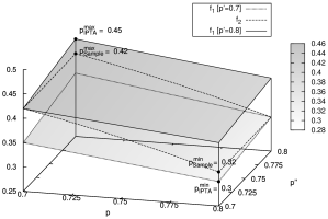
Figure 3: Analytic solutions for the property ‘one out of two response is slow’

The plane in the middle represents the solution for the sampling-based pta approach, which reaches a minimum probability of 0.32 for y=0.7 and a maximum probability of 0.42 for y=0.8. The upper and lower plane depict the IPTA version which reaches a minimum and maximum probabilities of 0.3 and 0.45, respectively. Therefore, the sampling approach using PTA is not sufficient for determining the correct minimum and maximum probabilities in the original IPTA model.

6.2 Encoding IPTA as PTA

Although the semantics of an interval distribution, i.e., the set of all probability distributions that respect the bounds of its intervals, is in general infinite, it is still possible to encode any finite IPTA into an equivalent, finite PTA. This encoding, which we also refer to as PTA$\!{}^{*}$, works as follows:

• The actions, clocks and locations of the PTA are the same as in the IPTA.

• For every transition $s{\,\xrightarrow{a}\,}\lambda$ in the IPTA and any ordering of the set $\mathit{Supp}(\lambda)$ add the transition $s{\,\xrightarrow{a}\,}\mu_{\lambda}^{\max}$ to the PTA (cf. Section 4.3).

As an example, Figure 4 depicts the PTA$\!{}^{*}$ encoding of the server IPTA in Figure 2. From the construction, it is clear that this encoding preserves probabilistic reachability, i.e., the minimum and maximum probabilities for reaching a set of target states in this PTA is the same as for the original IPTA. However, the number of generated transitions in the PTA is exponential in the size of the support of the transition. Thus, there is a significant blow-up in the size of the model. Even in our simple example in Figure 2 where the support sets have a size of at most 2, the larger number of transitions in the PTA$\!{}^{*}$ encoding results in longer run-times of the model checker. To illustrate this, we increased the number of requests performed by the client in our running example and compared the run-times of PRISM.

Figure 4: PTA$\!{}^{*}$ encoding of the server IPTA

6.3 Comparison of the run-times

Table 1 summarizes the run-times of our IPTA version of PRISM for three different encodings of the running example:

1. PTA: sampling approach where a single probability distribution in the interval distribution is tested;

2. IPTA: the original model as in Listing 2;

3. PTA$\!{}^{*}$: the encoding of the original IPTA using $\mu_{\lambda}^{\max}$;

#Requests	#States	PTA	IPTA	PTA$\!{}^{*}$
10	235	0.752	0.804	0.816
20	865	2.274	2.625	2.888
30	1,895	7.274	7.818	9.225
40	3,325	19.170	21.662	25.990
50	5,155	43.573	47.908	57.847

Table 1: Runtime in seconds for computing minimum probabilities for ‘less than 50% slow responses’

The checking of the PTA version was the fastest. However, we have shown above already that such a naive analysis using sampling does not produce the correct results. While the PTA$\!{}^{*}$ version yields the correct results, the numbers show that the direct checking of the IPTA is more efficient. This is due to the fact the number of transitions to be checked in PTA$\!{}^{*}$ encoding is higher than in the original IPTA. The actual numbers of the transitions in the example are listed in Table 2. Note that in our simple client/server example, the support sets of the transitions are very small (of size 1 or 2). We expect that with a greater branching of transitions, the performance loss using the PTA$\!{}^{*}$ encoding gets significantly worse.

#Requests	PTA	IPTA	PTA$\!{}^{*}$
10	339	339	521
20	1,269	1,269	2,031
30	2,799	2,799	4,541
40	4,929	4,929	8,051
50	7,659	7,659	12,561

Table 2: Number of transitions for different encodings of the client/server example

7 Related work

Probabilistic reachability and expected reachability for PTA based on an integral model of time (digital clocks) is studied in [12]. A zone-based algorithm for symbolic PTCTL [14] model checking of PTA is introduced in [14]. A notion of probabilistic time-abstracting bisimulation for PTA is introduced in [3]. For an overview of tools that support verification of (priced) PTA we refer to the related tools section in [11]. Interval-based probabilistic models and their use for specification and refinement / abstraction have been studied already in ’91 in [6]. PCTL model checking of interval Markov chains is introduced in [17]. Symbolic model checking for IPTA is presented in [19] based on the approaches in [14, 17]. However, no tool support or evaluation is given. Moreover, we show here that IPTA can also be encoded into PTA and provide some empirical data for comparing the differences in terms of correctness and run-times of our model checker.

Quality prediction of service compositions based on probabilistic model checking with PRISM is suggested in [5]. A comparison of different QoS models for service-oriented systems and an extension of the UML for quantitative models is given in [8]. A formal syntax for service level agreements of web services can be given using WSLA [9, 4]. A compositional QoS model for channel-based coordination of services is presented in [15].

8 Conclusions

We demonstrated in this paper how the recently introduced model of Interval Probabilistic Timed Automata [19] (IPTA) can be employed to model and verify quality of service guarantees, specifically, probabilistic real-time properties for service-oriented systems with dynamic service binding with contracts specified in service level agreements. We have shown that IPTA can capture the guarantees specified in the SLAs more naturally than PTA. To the best of our knowledge, our extension of the PRISM tool is the first implementation of an IPTA model checker. Moreover, we were able to show that IPTA can be analyzed nearly as fast as sample PTA and faster than a possible encoding of an IPTA in a finite PTA.

As future work, we plan to study refinement notions for IPTA which we hope will enable us to reason compositionally about QoS guarantees of service-oriented systems.

Acknowledgments

The authors of this paper are grateful to Dave Parker for his support with the IPTA implementation in PRISM.

References

- [1]
- [2] D. P. Bertsekas & J. N. Tsitsiklis (1991): An Analysis of Stochastic Shortest Path Problems. Mathematics of Operations Research 16(3), pp. 580–595, 10.1287/moor.16.3.580.
- [3] T. Chen, T. Han & J. P. Katoen (2008): Time-Abstracting Bisimulation for Probabilistic Timed Automata. In: TASE’08, IEEE Comp. Soc., pp. 177–184, 10.1109/TASE.2008.29.
- [4] A. Dan, R. Franck, A. Keller, R. King & H. Ludwig (2002): Web Service Level Agreement (WSLA) Language Specification. Available at http://www.research.ibm.com/wsla/documents.html.
- [5] S. Gallotti, C. Ghezzi, R. Mirandola & G. Tamburrelli (2008): Quality Prediction of Service Compositions through Probabilistic Model Checking. In: QoSA’08, LNCS 5281, Springer, pp. 119–134, 10.1007/978-3-540-87879-7_8.
- [6] B. Jonsson & K. G. Larsen (1991): Specification and Refinement of Probabilistic Processes. In: LICS’91, IEEE Comp. Soc., pp. 266–277, 10.1109/LICS.1991.151651.
- [7] M. Jurdzinski, J. Sproston & F. Laroussinie (2008): Model Checking Probabilistic Timed Automata with One or Two Clocks. Log. Meth. in Comp. Sci. 4(3), 10.2168/LMCS-4(3:12)2008.
- [8] I. Jureta, C. Herssens & S. Faulkner (2009): A comprehensive quality model for service-oriented systems. Software Quality Journal 17, pp. 65–98, 10.1007/s11219-008-9059-2.
- [9] A. Keller & H. Ludwig (2003): The WSLA Framework: Specifying and Monitoring Service Level Agreements for Web Services. J. Netw. Syst. Manage. 11, p. 2003, 10.1023/A:1022445108617.
- [10] J. Kemeny, J. Snell & A. Knapp (1976): Denumerable Markov Chains, 2nd edition. Springer.
- [11] M. Kwiatkowska, G. Norman & D. Parker (2011): PRISM 4.0: Verification of Probabilistic Real-time Systems. In: CAV’11, LNCS 6806, Springer, pp. 585–591, 10.1007/978-3-642-22110-1_47.
- [12] M. Kwiatkowska, G. Norman, D. Parker & J. Sproston (2006): Performance Analysis of Probabilistic Timed Automata using Digital Clocks. Form. Methods Syst. Des. 29, pp. 33–78, 10.1007/s10703-006-0005-2.
- [13] M. Kwiatkowska, G. Norman, R. Segala & J. Sproston (2002): Automatic verification of real-time systems with discrete probability distributions. Theor. Comput. Sci. 282, pp. 101–150, 10.1016/S0304-3975(01)00046-9.
- [14] M. Kwiatkowska, G. Norman, J. Sproston & F. Wang (2007): Symbolic model checking for probabilistic timed automata. Inf. Comput. 205, pp. 1027–1077, 10.1016/j.ic.2007.01.004.
- [15] Y.-J. Moon, A. Silva, C. Krause & F. Arbab (2011): A Compositional Model to Reason about end-to-end QoS in Stochastic Reo Connectors. Science of Computer Programming (to appear) .
- [16] PRISM Case Studies. http://www.prismmodelchecker.org/casestudies.
- [17] K. Sen, M. Viswanathan & G. Agha (2006): Model-Checking Markov Chains in the Presence of Uncertainties. In: TACAS’06, LNCS 3920, Springer, pp. 394–410, 10.1007/11691372_26.
- [18] UPPAAL Case Studies. http://www.it.uu.se/research/group/darts/uppaal/examples.shtml.
- [19] J. Zhang, J. Zhao, Z. Huang & Z. Cao (2009): Model Checking Interval Probabilistic Timed Automata. In: ICISE’09, IEEE Comp. Soc., pp. 4936–4940, 10.1109/ICISE.2009.749.