Synthesis of Switching Rules for Ensuring Reachability Properties of Sampled Linear Systems

Abstract

We consider here systems with piecewise linear dynamics that are periodically sampled with a given period $\tau$. At each sampling time, the mode of the system, i.e., the parameters of the linear dynamics, can be switched, according to a switching rule. Such systems can be modelled as a special form of hybrid automata, called “switched systems”, that are automata with an infinite real state space. The problem is to find a switching rule that guarantees the system to still be in a given area $V$ at the next sampling time, and so on indefinitely. In this paper, we will consider two approaches: the indirect one that abstracts the system under the form of a finite discrete event system, and the direct one that works on the continuous state space.
Our methods rely on previous works, but we specialize them to a simplified context (linearity, periodic switching instants, absence of control input), which is motivated by the features of a focused case study: a DC-DC boost converter built by electronics laboratory SATIE (ENS Cachan). Our enhanced methods allow us to treat successfully this real-life example.

1 Introduction

We are interested here in finding rules for switching the modes of (piecewise) linear systems in order to make the variables of the system stay within the limits of given area $V$. The systems that we consider are periodically sampled with a given period $\tau$. Between two sampling times, the variables follow a certain system of linear differential equations, corresponding to a mode among several other ones. At each sampling time, the mode of the system can be switched. Such systems can be modelled as a special form of hybrid automata, called “switched systems”, that are automata with an infinite real state space. The problem that we consider here is to find a switching rule that selects a mode ensuring that the system will still be in $V$ at the next sampling time, and so on indefinitely.

Note that, here, we do not impose that the systems always lies within $V$ between two sampling times, only at sampling times: if the system goes out of $V$ between two sampling times, then, due to continuity reasons and because of the “small” size of $\tau$, it will still stay within the close neighborhood of $V$, and we assume that such a small deviation is acceptable for the system. This makes the problem simpler than the one considered, e.g. in [abdmp00], where the system is forced to always stay within $V$.

Note also that the problem here is simpler than the one considered in [sun-ge-lee02], because, here, only the switching rule has to be determined, since the control input is fixed. (In [sun-ge-lee02], the dynamics is of the form $\dot{x}(t)=A{x}(t)+Bu(t)$, where $u(t)$ is not constant, but an input to be synthesized.)

Finally, our problem is much simplified by the fact that, as in [Girard], the switching instants can only occur at times of the form $i\tau$ with $i\in\mathbb{N}$.

As noted in [abdmp00], there are two approaches for solving this kind of problem:

- the indirect approach reduces first the system, via abstraction, into a discrete event system (typically, a finite-state automaton); this is done in, e.g., [Girard]. One can thus identify cycles in the graph of the abstract system, thus inferring possible patterns of modes that enforces the system to stay forever within $V$.

- the direct approach works directly on the continuous state space; this is done, e.g., in [abdmp00]. One can thus infer a controllable subspace $V^{\prime}$ of $V$, within which the existence of a switching rule allowing to stay forever within $V^{\prime}$ is guaranteed (see, e.g., [sun-ge-lee02, krastanov-veliov04]).

Often, in the indirect approach, the switching rule can be computed off line (under, e.g., the form of a repeated pattern of modes), while the switching rule has to be computed on line in the direct approach.

Our methods basically rely on previous works, but we specialize them to the simplified context (linearity, periodic switching instants, absence of control input), which is motivated by the features of a focused case study: a DC-DC boost converter built by electronics laboratory SATIE (ENS Cachan) for the automative industry. Our enhanced methods allow us to treat successfully this real-life example.

2 Indirect Approach: Approximately Bisimular Methods

2.1 Sampled Switched Systems

In this paper, we consider a subclass of hybrid systems [Henzinger], called “switched systems” in [Girard].

Definition 1

A switched system $\Sigma$ is a quadruple $(\mathbb{R}^{n},P,\mathcal{P},F)$ where:

• $\mathbb{R}^{n}$ is the state space

• $P=\{1,\dots,m\}$ is a finite set of modes,

• ${\cal P}$ is a subset of ${\cal S}(\mathbb{R}_{\geq 0},P)$ which denotes the set of piecewise constant functions from $\mathbb{R}_{\geq 0}$ to $P$, continuous from the right and with a finite number of discontinuities on every bounded interval of $\mathbb{R}_{>0}$

• $F=\{f_{p}\ |\ p\in P\}$ is a collection of functions indexed by $P$.

For all $p\in P$, we denote by $\Sigma_{p}$ the continuous subsystem of $\Sigma$ defined by the differential equation:

$$\dot{{\bf x}}(t)=f_{p}({\bf x}(t)).$$

A switching signal of $\Sigma$ is a function ${\bf p}\in{\cal P}$, the discontinuities of ${\bf p}$ are called switching times. A piecewise ${\cal C}^{1}$ function ${\bf x}:\mathbb{R}_{>0}\rightarrow\mathbb{R}^{n}$ is said to be a trajectory of $\Sigma$ if it is continuous and there exists a switching signal ${\bf p}\in{\cal P}$ such that, at each $t\in\mathbb{R}_{>0}$, ${\bf x}$ is continuously differentiable and satisfies:

$$\dot{{\bf x}}(t)=f_{{\bf p}(t)}({\bf x}(t)).$$

We will use ${\bf x}(t,x,{\bf p})$ to denote the point reached at time $t\in\mathbb{R}_{>0}$ from the initial condition $x$ under the swiching signal ${\bf x}$. Let us remark that a trajectory of $\Sigma_{p}$ is a trajectory of $\Sigma$ associated with the constant signal ${\bf x}(t)=p$, for all $t\in\mathbb{R}_{>0}$.

In this paper, we focus on the case of linear switched systems: for all $p\in P$, the function $f_{p}$ is defined by $f_{p}(x)=A_{p}x+b_{p}$ where $A_{p}$ is a $(n\times n)$-matrix of constant elements $(a_{i,j})_{p}$ and $b_{p}$ is a $n$-vector of constant elements $(b_{k})_{p}$.

In the following, as in [Girard], we will work with trajectories of duration $\tau$ for some chosen $\tau\in\mathbb{R}_{\geq 0}$, called “time sampling parameter”. This can be seen as a sampling process. Particularly, we suppose that switching instants can only occur at times of the form $i\tau$ with $i\in\mathbb{N}$. In the following, we will consider transition systems that describe trajectories of duration $\tau$, for some given time sampling parameter $\tau\in\mathbb{R}_{\geq 0}$.

Definition 2

Let $\Sigma=(\mathbb{R}^{n},P,{\cal P},F)$ be a switched system and $\tau\in\mathbb{R}_{\geq 0}$ a time sampling parameter. The $\tau$-sampled transition system associated to $\Sigma$, denoted by $T_{\tau}(\Sigma)$ , is the transition system $(Q,\rightarrow^{p}_{\tau})$ defined by:

• the set of states is $Q=\mathbb{R}^{n}$

• the transition relation is given by

  $$x\rightarrow^{p}_{\tau}x^{\prime}\mbox{ iff }{\mathbb{x}}(\tau,x,p)=x^{\prime}$$

Let us define: $Post_{i}(X)=\{x^{\prime}\ |\ x\rightarrow^{i}_{\tau}x^{\prime}\mbox{ for some $x\in X$}\}$, and
$Pre_{i}(X)=\{x^{\prime}\ |\ x^{\prime}\rightarrow^{i}_{\tau}x\mbox{ for some $x\in X$}\}$. For the sake of brevity, we will use $Post_{i}(x)$ instead of $Post_{i}(\{x\})$ and $Pre_{i}(x)$ instead of $Pre_{i}(\{x\})$.

Example 1

This example is a boost DC-DC converter with one switching cell (see Fig. 1) that is taken from [Girard] (see also, e.g., [BecPap:2005:IFA_2345, test, Senesky03hybridmodeling]). The boost converter has two operation modes depending on the position of the switching cell. The state of the system is $x(t)=[i_{l}(t),v_{c}(t)]^{T}$ where $i_{l}(t)$ is the inductor current and $v_{c}(t)$ the capacitor voltage. The dynamics associated with both modes are of the form $\dot{x}(t)=A_{p}x(t)+b_{p}$ ($p=1,2$) with

$$A_{1}=\begin{pmatrix}-\frac{r_{l}}{x_{l}}&0\\ 0&-\frac{1}{x_{c}}\frac{1}{r_{0}+r_{c}}\end{pmatrix}\ \ \ b_{1}=\begin{pmatrix}\frac{v_{s}}{x_{l}}\\ 0\end{pmatrix}$$

$$A_{2}=\begin{pmatrix}-\frac{1}{x_{l}}(r_{l}+\frac{r_{0}.r_{c}}{r_{0}+r_{c}})&-\frac{1}{x_{l}}\frac{r_{0}}{r_{0}+r_{c}}\\ \frac{1}{x_{c}}\frac{r_{0}}{r_{0}+r_{c}}&-\frac{1}{x_{c}}\frac{r_{0}}{r_{0}+r_{c}}\end{pmatrix}\ \ \ b_{2}=\begin{pmatrix}\frac{v_{s}}{x_{l}}\\ 0\end{pmatrix}$$

It is clear that the boost converter is an example of a switched system. We will use the numerical values of [Girard]: $x_{c}=70$, $x_{l}=3$, $r_{c}=0.005$, $r_{l}=0.05$, $r_{0}=1$, $v_{s}=1$. The goal of the boost converter is to regulate the output voltage across the load $r_{0}$. This control problem is usually reformulated as a current reference scheme. Then, the goal is to keep the inductor current $i_{l}(t)$ around a reference value $i_{l}^{ref}$. This can be done, for instance, by synthesizing a controller that keeps the state of the switched system in an invariant set centered around the reference value. An example of switching rule is illustrated on Fig. 2. This rule is periodic of period $T_{d}$: the mode is 2 on $(0,\frac{T_{d}}{4}]$ and 1 on $(\frac{T_{d}}{4},T_{d}]$. A.

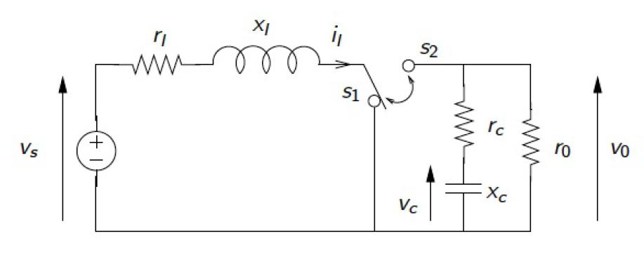
Figure 1: Electric scheme of the boost DC-DC converter (1 cell)

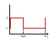
Figure 2: A switching rule for the 1-cell boost DC-DC converter on one period of length $T_{d}$ (here, $\tau=\frac{T_{d}}{4}$, and the pattern of the switching rule is $(2.1.1.1)$)

2.2 Approximate bisimulation

In [Girard], the authors propose a method for abstracting a switched system under the form of a discrete symbolic model, that is equivalent to the original one, under certain Lyapunov-based stability conditions. They use an Euclidian metric $\|.\|$, and define the approximation of the set of states $\mathbb{R}^{n}$ as follows:

$$[\mathbb{R}^{n}]_{\eta}=\{x\in\mathbb{R}^{n}\ |\ x_{i}=k_{i}\frac{2\eta}{\sqrt{n}},\ k_{i}\in\mathbb{Z},i=1,\dots,n\},$$

where $\eta\in\mathbb{R}_{\geq 0}$ is a state space discretization parameter. The transition relation $T_{\tau}(\Sigma)$ is approximated as follows: Let $q\in[\mathbb{R}^{n}]_{\eta}$ and $q_{e}={\bf x}(\tau,q,p)$ such that $q\rightarrow_{T_{\tau}(\Sigma_{p})}q_{e}$ in the real system, let $q^{\prime}\in[\mathbb{R}^{n}]_{\eta}$ with $||q_{e}-q^{\prime}||<\eta$. Then we have $q\rightarrow_{T_{\tau,\eta}(\Sigma_{p})}q^{\prime}$ for the approximated transition relation. The approximate transition system $T_{\tau,\eta}(\Sigma)$ is defined as follows:

Definition 3

The system $T_{\tau,\eta}(\Sigma)$ is the transition system $(Q,\rightarrow^{p}_{\tau,\eta})$ defined by:

• the set of states is $Q=[\mathbb{R}^{n}]_{\eta}$

• the transition relation is given by

  $$q\rightarrow^{p}_{\tau,\eta}q^{\prime}\mbox{ iff }\|{\mathbb{x}}(\tau,q,p)-q^{\prime}\|\leq\eta$$

  where $\|.\|$ is any metric on $\mathbb{R}^{n}$.

The notion of “approximate bisimilarity” between systems $T_{\tau}(\Sigma)$ and $T_{\tau,\eta}(\Sigma)$ is defined as follows:

Definition 4

Systems $T_{\tau}(\Sigma)$ and $T_{\tau,\eta}(\Sigma)$ are $\varepsilon$-bisimilar if:

1. $(\|x-q\|\leq\varepsilon\wedge q\rightarrow^{p}_{\tau,\eta}q^{\prime})\ \ \Rightarrow\ \ \|x^{\prime}-q^{\prime}\|\leq\varepsilon$
   for some $x^{\prime}={\mathbb{x}}(\tau,x,p)$ (i.e. for some ${\bf x}^{\prime}:$ $x\rightarrow^{p}_{\tau}x^{\prime}$), and

2. $(\|x-q\|\leq\varepsilon\wedge x\rightarrow^{p}_{\tau}x^{\prime})\ \ \Rightarrow\ \ \|x^{\prime}-q^{\prime}\|\leq\varepsilon$
   for some $q^{\prime}\in[\mathbb{R}^{n}]_{\eta}:\|{\mathbb{x}}(\tau,q,p)-q^{\prime}\|\leq\eta$ (i.e. for some $q^{\prime}:$ $q\rightarrow^{p}_{\tau,\eta}q^{\prime}$).

The following theorem is given in [Girard].

Theorem 1

Consider a switched system $\Sigma=(\mathbb{R}^{n},P,{\cal P},F)$ with ${\cal P}={\cal S}(\mathbb{R}^{+},P)$, a desired precision $\varepsilon$ and a time sampling value $\tau$. Under certain Lyapunov-based stabilization conditions, there exists a space sampling value $\eta$ such that the transition systems $T_{\tau}(\Sigma)$ and $T_{\tau,\eta}(\Sigma)$ are approximately bisimilar with precision $\varepsilon$.

One can guarantee an arbitrary precision $\varepsilon$ by choosing an appropriate $\eta$: there exists an explicit algebric relation between $\varepsilon$ and $\eta$. Furthermore, under certain conditions (stability of $T_{\tau}(\Sigma)$), the symbolic model $T_{\tau,\eta}(\Sigma)$ has a finite number of states. One can then use standard techniques of model checking in order to synthesize a safe switching rule on $T_{\tau,\eta}(\Sigma)$ (e.g., letting the system always in the safe area), see e.g. [AVW03, RW89]. The switching rule on $T_{\tau,\eta}(\Sigma)$ can also be used to enforce the real system $T_{\tau}(\Sigma)$ to behave correctly.

2.3 Simplification for the Case of Linear Dynamics

By focusing on linear dynamics, we are allowed to simplify the more general method of [Girard] as follows:

1. We are using the infinity norm in order to remove the overlapping of two adjacents bowls of radius $\eta$ (reducing it to a set with a norm 0). This is done to prevent non-determinism. Therefore, $[\mathbb{R}^{n}]_{\eta}$ has to be changed according to the use of this norm. From now on, $[\mathbb{R}^{n}]_{\eta}=\{x\in\mathbb{R}^{n}\ |\ x_{i}=2k\eta\ k\in\mathbb{Z}\}$

2. The computation of Lyapunov functions are not necessary in our particular case but can be done by simply computing the infinite sum of a geometric serie to ensure the $\varepsilon$-bisimulation. Stability criterion relies simply on the eigenvalues of matrices $A_{i}$ having negative real part. The proof of $\varepsilon$-bisimilarity is based on the fact that $\beta_{\tau}\varepsilon+\eta\leq\varepsilon$ (which is true for some $\eta$ when $\beta_{\tau}<1$) (See [rr-lsv-11-12] for more details).

3. Due to the presence of the exponential of a matrix, the computation of the image of all the points could be very costly. By using the linearity of the system, we can compute the same results for a fraction of the initial cost. This is explained in [rr-lsv-11-12].

Example 2

Our simplified method is applied on the boost converter of Example 1: $\tau=0.5$, $V$ corresponding to $i_{l}\in[3,3.4]$ and $v_{c}\in[1.5,1.8]$, $\varepsilon=3.0$, $\eta=1/40$.. See Fig. 3 for one of the connected component of the full graph. Each cycle in the graph corresponds to a periodic control of the converter which ensures that the electric variables lie inside the predefined $V$ up to $\varepsilon$. For example, we consider the cycle going through the vertices: $159,243,173,257,187,271,201,285,215,299,\\ 229,159$. This corresponds to the periodic mode control of pattern $12121212122$. The result of a simulation under this periodic switching rule is given in Fig. 4 for a starting point $x_{0}=(3.0,1.79)$. The box $V$ is delimited by the red lines. One can see that the system largely exceeds the limits of $V$ (but stays inside the $\varepsilon$-approximation).

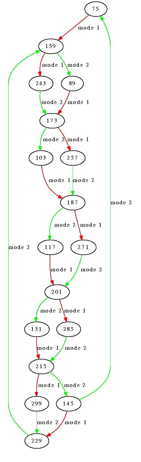
Figure 3: Synthesized finite-state automaton for 1-cell converter with $\eta=\frac{1}{40}$ and $V$ corresponding to $i_{l}\in[3,3.4]$ and $v_{c}\in[1.5,1.8]$

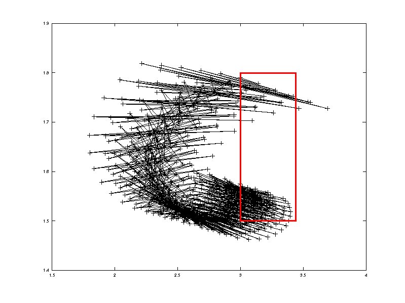
Figure 4: Projected simulation with $i_{l}$ on the abscissa, and $v_{c}$ on the ordinates of 1-cell converter for switching rule $(12121212122)^{*}$ starting point $x_{0}=(3.0,1.79)$ ; The box $V=[3,3.4]\times[1.5,1.8]$ is drawn in red. ($\varepsilon=2.6$)

3 Direct Approach: Inference of Controllable Subspace

The direct approach works directly on the continuous state space; this is done, e.g., in [abdmp00]. One can thus infer a controllable subspace $V^{\prime}$ of $V$, within which the existence of a switching rule allowing to stay forever within $V^{\prime}$ is guaranteed (see, e.g., [sun-ge-lee02, krastanov-veliov04]). We present here a simplified direct method that exploits the simple features of our framework: linearity, absence of perturbation $u$, periodicity of the switching instants.

Consider a box $V\subset\mathbb{R}^{n}$ and a time sampling value $\tau$. The following Algorithm 1 computes a set of controllable polyhedra. Intuitively, after the $k^{th}$ iteration of the loop, $Control_{i}$ is a set of states satisfying the following property: there exists a sequence of modes $\sigma$ of length $k$ starting with mode $i$ such that $\sigma$ applied to any state of $Control_{i}$ prevents the system to go out of $V$ at any sampling time; alternatively, after the $k^{th}$ iteration, $Uncontrol$ is a set of states for which, for all sequence $\sigma$, there exists a prefix $\sigma^{\prime}$ which makes the system go outside $V$. Note that the termination of the procedure is not guaranteed due to the fact that there are infinitely many polyhedral sets.

1

input : A switched system $\Sigma$ with $m$ modes

input : A time sampling value $\tau$

input : A box $V\subset\mathbb{R}^{n}$

2

output : A controllable subspace $V^{\prime}=\{Control_{i}\}_{i=1..m}$

3 $Uncontrol_{new}:=V$

4 for $i=1..m$ do

5       $Control_{i}:=V$

6repeat

7       $Uncontrol:=Uncontrol_{new}$

8       for $i=1..m$ do

9            $Control_{i}:=Control_{i}\setminus Pre_{i}(Uncontrol)$

10      $Uncontrol_{new}:=V\setminus\bigcup_{i=1}^{m}Control_{i}$

11until $Uncontrol_{new}=Uncontrol$;

12return $V^{\prime}=\bigcup_{i=1}^{m}Control_{i}$

Algorithm 1 Synthesis of controllable subspace

The correctness of Algorithm 1 relies on the following fact:

Theorem 2

If Algorithm 1 terminates with output $V^{\prime}$, then $Post_{i}(V^{\prime})\subseteq V^{\prime}$ for all $1\leq i\leq m$.

In order to prove Theorem 2, we need the two following propositions.

Proposition 1

Let $x,x^{\prime}\in\mathbb{R}^{n}$. Then the three following items are equivalent:

• $x=x^{\prime}$

• $Post_{i}(x)=Post_{i}(x^{\prime})$ for all $1\leq i\leq m$

• $Pre_{i}(x)\neq Pre_{i}(x^{\prime})$ for all $1\leq i\leq m$

Proof
We only consider Linear Differential Equations, for any $x\in\mathbb{R}^{n}$ $Card(Post_{i}(x))=Card(Pre_{i}(x))=1$. The proof is immediate from Cauchy-Lipschitz Theorem. $\Box$

Proposition 2

Let $A,B\subseteq\mathbb{R}^{n}$. We have:

1. $Post_{i}(A\setminus B)=Post_{i}(A)\setminus Post_{i}(B)$ and similary for $Pre_{i}$ for all $1\leq ileqm$.

2. $Post_{i}(Pre_{i}(A))=Pre_{i}(Post_{i}(A))=A$.