An Approach using Demisubmartingales for the Stochastic Analysis of Networks

Abstract

Stochastic network calculus is the probabilistic version of the network calculus, which uses envelopes to perform probabilistic analysis of queueing networks. The accuracy of probabilistic end-to-end delay or backlog bounds computed using network calculus has always been a concern. In this paper, we propose novel end-to-end probabilistic bounds based on demisubmartingale inequalities which improve the existing bounds for the tandem networks of GI/GI/1 queues. In particular, we show that reasonably accurate bounds are achieved by comparing the new bounds with the existing results for a network of M/M/1 queues.

I Introduction

Queueing theory is the mathematical study of queues, which generally uses probability mass or density functions to describe arrival traffic and service offered at the network node to compute probabilistic delay or backlog measures. However, with few exceptions, analysis of queueing networks to compute end-to-end probabilistic performance measures is mathematically complex without making simplifying assumptions on arrival traffic or service offered at the network nodes. In most situations, probabilistic bounds on performance measures are as sufficient as the actual values. Deterministic network calculus is an elegant theory, useful for computing worst-case bounds on end-to-end delay or backlog in queueing networks. Stochastic network calculus is the probabilistic extension of deterministic network calculus, which uses an envelope approach to describe arrival traffic and service offered at the network node. The tightness of the end-to-end probabilistic performance bounds has always been a concern in stochastic network calculus. The concern is mainly due to the use of union bounds for computing the bounds on probabilistic performance measures of the network. Recently, in [1, 2], authors have derived new performance bounds for a GI/GI/1 queue in stochastic network calculus using Doob’s maximal inequality for exponential supermartingales (instead of using union bounds) which are comparable to the exact results of M/M/1 and M/D/1 queues from queueing theory. A general comparison of results for GI/GI/1 queue from statistical network calculus with the classical queueing theory is made in [3].

In this paper, we compute end-to-end probabilistic performance bounds for tandem networks of GI/GI/1 queues in stochastic network calculus using demisubmartingale inequalities [4, 5]. The key difference of the approach used in this paper to the work presented in [1, 2] is that we derive performance bounds for a GI/GI/1 queue using statistical envelopes, in contrast to using stochastic processes as in [1, 2]. The rest of the paper is structured as follows: In Section II, we introduce the notion and assumptions used in the paper. In Section III, we derive the probabilistic end-to-end performance bounds on delay and backlog for the tandem networks of GI/GI/1 queues using statistical envelopes. Brief conclusions are presented in Section IV.

II Notation and Assumptions

Our time model is discrete, i.e., $t\in\mathbb{N}_{0}=\{0,1,2,\ldots\}$. We assume that the arrival traffic and the service offered at a node are stationary and have independent increments. In a network of nodes connected in series as shown in Fig. 1, we use non-decreasing, left-continuous processes $A_{h}$ and $D_{h}$ to describe the arrivals and the departures at node $h$, respectively. $A_{h}(s,t)$ and $D_{h}(s,t)$ represent the cumulative amount of data seen in an interval $(s,t]$ at input and output of node $h$, respectively, for any $0\leq s\leq t$. For the arrival and departure processes at node $h$, we assume the initial condition $A_{h}(t)=0$ for $t\in(-\infty,0]$ and the causal condition $D_{h}(t)\leq A_{h}(t)$, where we denote $A_{h}(0,t)=A_{h}(t)$ and $D_{h}(0,t)=D_{h}(t)$ for any $t\geq 0$. The backlog $B_{h}(t)$ and delay $W_{h}(t)$ at time $t\geq 0$ in a node $h$ are given by $B_{h}(t)=A_{h}(t)-D_{h}(t)$ and $W_{h}(t)=\inf{\{d\geq 0:A_{h}(t-d)\leq D_{h}(t)\}}$, respectively.

A stochastic process $S_{h}$ is said to describe the service offered at node $h$, if the corresponding arrival and departure processes at node $h$ satisfy for any fixed sample path and $t\geq 0$:

$$A_{h}\otimes S_{h}(t)\leq D_{h}(t)$$ (1)

where $\otimes$ is the min-plus convolution of $A_{h}$ and $S_{h}$ which is defined as $A_{h}\otimes S_{h}(t)=\inf_{0\leq u\leq t}\{A_{h}(0,u)+S_{h}(u,t)\}$. Any random process $S$ satisfying the above relationship is referred to as “dynamic F-server” in [6].

The arrival and the service processes are described using statistical envelopes in network calculus. A statistical arrival envelope ${\cal G}$ for an arrival process $A$ is defined as a non-negative function for all $t\geq 0$ satisfying the following condition

$$P\{A(t)-{\cal G}(t)>\sigma\}\leq\varepsilon_{{\cal G}}(\sigma)$$ (2)

where $\varepsilon_{{\cal G}}$ is a non-increasing error function bounding the violation probability of the statistical arrival envelope. Similarly, a statistical service envelope ${\cal S}$ describing the service offered at the network node with arrival traffic $A$ and departure traffic $D$ is defined as a non-negative function for all $t\geq 0$ satisfying the following condition

$$P\{A\otimes{\cal S}(t)-D(t)>\sigma\}\leq\varepsilon_{{\cal S}}(\sigma)$$ (3)

where $\varepsilon_{{\cal S}}$ is a non-increasing error function bounding the violation probability of the statistical service envelope. The statistical service envelope from equation (3) is related to the service process from equation (1) for all $t\geq 0$ by the following expression

$$P\{{\cal S}(t)-S(t)>\sigma\}\leq\varepsilon_{{\cal S}}(\sigma)$$ (4)

In this paper, we use the notion of effective bandwidth ($\alpha$) [7] and effective capacity ($\beta$) [8, 9, 10] from large deviations theory to derive statistical arrival and service envelopes describing the stochastic arrival traffic and the service offered at a node, respectively. The effective bandwidth of an arrival traffic $A$ with independent increments from [7], for any $\theta,t>0$, is given as

$$\alpha(\theta)=\frac{1}{\theta}\log{E\left[e^{\theta A(1)}\right]}$$ (5)

Similarly, the effective capacity function of a stochastic service process $S$ with independent increments, for any $\theta,t>0$, is defined as

$${\beta}(\theta)=-\frac{1}{\theta}\log{E\left[e^{-\theta S(1)}\right]}$$ (6)

Then the statistical arrival and service envelopes in terms of effective bandwidth of the probabilistic arrival process and effective capacity of the service process observed at a network node are given as ${\cal G}(t)=\alpha(\theta)t$ and ${\cal S}(t)=\beta(\theta)t$, respectively, for any given $\theta\geq 0$; they satisfy the appropriate conditions in equations (2) and (4) with the error function $\varepsilon(\sigma)=e^{-\theta\sigma}$.

Figure 1: Network of H concatenated nodes

The main advantage of using network calculus to do performance analysis of networks is that the network calculus allows to model a network of nodes as a single virtual node. The stochastic network service process $S_{net}$ characterizing the service offered in a single virtual network node, which represents a network of $H$ nodes connected in series as shown in Fig.1, can be computed for any fixed sample path using the min-plus convolution of the stochastic service process $S_{h}$ of constituting nodes for $h=1,\ldots,H$, i.e., $S_{net}=S_{1}\otimes S_{2}\otimes\cdots\otimes S_{H}$ [6, 11]. The corresponding statistical network service envelope is given as ${\cal S}_{net}={\cal S}_{1}\otimes{\cal S}_{2}\otimes\cdots\otimes{\cal S}_{H}$, where ${\cal S}_{h}$ is the statistical service envelope describing the service offered at node $h$, for $h=1,2,\ldots,H$. We assume that the arrival traffic $A_{1}$ at the ingress of the network and the stochastic service processes $S_{h}$, for $h=1,\ldots,H$, characterizing the service offered at the nodes of the network are independent of each other.

III Probabilistic Bounds on Backlog and Delay

In this section, we compute probabilistic bounds on backlog and delay in a network of $H$ nodes as shown in Fig. 1 using demisubmartingale inequalities. Let $A_{1}=A$ and $D_{H}=D$ be the arrival traffic at the ingress of the network and departure traffic from the egress of the network, respectively. The following theorem provides the probabilistic bounds on end-to-end backlog and delay using the statistical envelopes of arrival and service processes at each network node $h$, respectively.

Theorem III.1

Let the service offered at node $h$ in a tandem network be characterized by the stochastic service process $S_{h}$ with the corresponding effective capacity function $\beta_{h}$, for $h=1,\ldots,H$. Let $A$ be the arrival process with effective bandwidth $\alpha$ and $D$ be the departure process from the tandem network with $H$ nodes. Then we have the following bounds.

1. Backlog bound : The probabilistic bound on the backlog in a network, for any $t\geq 0$, is given by

   $$P\left\{B(t)>x\right\}\leq\tilde{\varepsilon}(x)$$ (7)

2. Delay bound : The probabilistic bound on the delay in a network, for any $t\geq 0$, is given by

   $$P\left\{W(t)>d\right\}\leq\tilde{\varepsilon}(\alpha(\theta^{*})d)$$ (8)

where $\tilde{\varepsilon}$ is an error function, for any $x\geq 0$, given as:

$$\tilde{\varepsilon}(x)=\begin{cases}\ \ \ \ \ \ \ \ \ \ \ \ \ \ \ \ \ \ \ \ \ e^{-\theta^{*}x}&\text{if }H=1\\ e^{-(\theta^{*}x-(H-1))}\sum_{h=0}^{H}{\frac{(\theta^{*}x-(H-1))^{h}}{h!}}&\text{if }H>1\\ &\text{and }x\geq\frac{H-1}{\theta^{*}}\end{cases}$$ (9)

and $\theta^{*}=\sup{\{\theta:\alpha(\theta)\leq\min_{1\leq h\leq H}{\{\beta_{h}(\theta)\}}\}}$.

The proof of the theorem relies on applying demisubmartingale inequalities to compute probabilistic bounds. The key observation is that certain functions of the random arrival and service processes together with their corresponding statistical envelopes form demisubmartingales. This is shown using the following lemma.

Lemma III.1

Let $A$ be the arrival traffic with effective bandwidth $\alpha$ at a network node offering a stochastic service characterized by a service process $S$ with effective capacity $\beta$. If the arrival and the service processes have stationary independent increments, then the random processes $X(t)=e^{\theta(A(t)-\alpha(\theta)t)}$, $Y(t)=e^{-\theta(S(t)-\beta(\theta)t)}$, $Z(t)=e^{-\theta^{*}(S(t)-A(t))}$ and $Y^{*}(t)=\sup_{0\leq u\leq t}Y(u)$ are demisubmartingales in an interval $[0,t]$ for $t\in\mathbb{N}_{0}=\{0,1,2,\ldots\}$ and any $\theta\in(0,\theta^{*}]$, where $\theta^{*}=\sup{\{\theta:\alpha(\theta)\leq\beta(\theta)\}}$.

Proof: To prove that $X(t)$, $Y(t)$, $Z(t)$ and $Y^{*}(t)$ are demisubmartingales [4, 5] for $t\in\mathbb{N}_{0}=\{0,1,2,\ldots\}$ and any $\theta\in(0,\theta^{*}]$ , we need to show that $E[(X(t+1)-X(t))f(X(1),X(2),\ldots,X(t))]\geq 0$, and corresponding statements hold for $Y(t),Z(t)$ and $Y^{*}(t)$ for $t\in\mathbb{N}_{0}=\{0,1,2,\ldots\}$ and every co-ordinatewise non-decreasing, non-negative function $f$ whenever the expectation is defined. As the proof for $X(t)$ follows the same lines as $Y(t)$, we will provide the proofs only for $Y(t)$, $Z(t)$ and $Y^{*}(t)$.

$$E[(Y(t+1)-Y(t))f(Y(1),Y(2),\ldots,Y(t))]$$

$$= E[(e^{\theta(\beta(\theta)-S(t,t+1))}-1)Y(t)f(Y(1),Y(2),\ldots,Y(t))]$$

$$= E[e^{\theta(\beta(\theta)-S(t,t+1))}-1]E[g(Y(1),Y(2),\ldots,Y(t))]=0$$

The last two equalities are due to the fact that the process $Y(t)$ has independent increments and $E[e^{-\theta S(t,t+1)}]=e^{-\theta\beta(\theta)}$ (cf., equation (6)), respectively. This proves that $Y(t)$ is a demisubmartingale (also a N-demisupermartingale).

$$E[(Z(t+1)-Z(t))f(Z(1),Z(2),\ldots,Z(t))]$$

$$= E[(e^{-\theta^{*}(S(t,t+1)-A(t,t+1))}-1)Z(t)f(Z(1),\ldots,Z(t))]$$

$$= (e^{-\theta^{*}\{\beta(\theta^{*})-\alpha(\theta^{*})\}}-1)E[g(Z(1),\ldots,Z(t))]=0$$

Equality at the second step is due to our assumption that the arrival $A(t)$ and service $S(t)$ processes have independent increments and $E[e^{-\theta S(t,t+1)}]=e^{-\theta\beta(\theta)}$, $E[e^{\theta A(t,t+1)}]=e^{\theta\alpha(\theta)}$. The last equality is from stability condition and the definition of $\theta^{*}$. This proves that $Z(t)$ is a demisubmartingale (also a N-demisupermartingale).

$$E[(Y^{*}(t+1)-Y^{*}(t))f(Y^{*}(1),Y^{*}(2),\ldots,Y^{*}(t))]$$

$$= E[(\max{\{Y^{*}(t),e^{\theta(\beta(\theta)-S(t,t+1))}\}}-Y^{*}(t))$$

$$\ \ \ \ \ \ \ \ \ \ \ \ \ \ \ \ \ \ \ \ \ \ \ \ \ \ \ \ f(Y^{*}(1),Y^{*}(2),\ldots,Y^{*}(t))]$$

$$= E[\max{\{0,e^{\theta(\beta(\theta)-S(t,t+1))}-Y^{*}(t)\}}$$

$$\ \ \ \ \ \ \ \ \ \ \ \ \ \ \ \ \ \ \ \ \ \ \ f(Y^{*}(1),Y^{*}(2),\ldots,Y^{*}(t))]\geq 0$$

This proves that $Y^{*}(t)$ is a demisubmartingale.$\blacksquare$
By Doob’s maximal inequality for demisubmartingales [4, 5], we have the following maximal inequalities for any $\theta,\sigma\geq 0$,

$$P\left\{\sup_{0\leq u\leq t}X(u)>e^{\theta\sigma}\right\} \leq E[X(t)]e^{-\theta\sigma}=e^{-\theta\sigma}$$ (10)

$$P\left\{\sup_{0\leq u\leq t}Y(u)>e^{\theta\sigma}\right\} \leq E[Y(t)]e^{-\theta\sigma}=e^{-\theta\sigma}$$ (11)

$$P\left\{\sup_{0\leq u\leq t}Z(u)>e^{\theta^{*}\sigma}\right\} \leq E[Z(t)]e^{-\theta^{*}\sigma}=e^{-\theta^{*}\sigma}$$ (12)

$$P\left\{\sup_{0\leq v\leq u\leq t}Y(v,u)>e^{\theta\sigma}\right\} = P\left\{\sup_{0\leq u\leq t}Y^{*}(u)>e^{\theta\sigma}\right\}$$ (13)

$$\leq E[Y^{*}(t)]e^{-\theta\sigma}$$

$$\leq eE[Y(t)]e^{-\theta\sigma}=ee^{-\theta\sigma}$$

The final inequality step is due to Rao’s maximal inequality for demisubmartingales (Theorem $3.7$ from [5]). The proof of Theorem III.1 also relies on Lemma 4.1 from [12], which states that for any two non-negative independent random variables $F$ and $G$ with $P(F>\sigma)\leq f(\sigma)$ and $P(G>\sigma)\leq g(\sigma)$ where $f(\sigma)$ and $g(\sigma)$ are non-negative, decreasing functions for any $\sigma\geq 0$, then

$$P\left\{F+G>\sigma\right\}\leq 1-\int_{0}^{\sigma}{\tilde{f}(\sigma-u)d\tilde{g}(u)}$$ (14)

where $\tilde{f}(\sigma)=1-\left[f(\sigma)\right]^{-}$, $\tilde{g}(\sigma)=1-\left[g(\sigma)\right]^{-}$ and $[a]^{-}=\min(1,a)$ for any $a\geq 0$.
Proof of Theorem III.1: We now provide the proof for the probabilistic end-to-end delay bound. The proof for the probabilistic bound on end-to-end backlog is its immediate variation. For single hop ($H=1$), the proof is straight forward and can be shown for fixed sample path, $t\geq 0$ and $\theta>0$ as follows:

$$P\left\{W(t)>d\right\}=P\left\{A(t-d)-D(t)>0\right\}$$ (15)

$$= P\left\{A(t-d)-D(t)>0\right\}$$

$$\leq P\left\{A(t-d)-A\otimes S_{1}(t)>0\right\}$$

$$= P\left\{\sup_{0\leq u\leq t-d}\{A(u,t-d)-S_{1}(u,t)\}+\alpha(\theta^{*})d>\alpha(\theta^{*})d\right\}$$

$$= P\left\{\sup_{0\leq u\leq t-d}\left\{e^{\theta^{*}\{A(u,t-d)-S_{1}(u,t)+\alpha(\theta^{*})d\}}\right\}>e^{\theta^{*}\alpha(\theta^{*})d}\right\}$$

$$\leq E\left[e^{\theta^{*}\{A(0,t-d)-S_{1}(0,t-d)-S_{1}(t-d,t)+\alpha(\theta^{*})d}\right]e^{-\theta^{*}\alpha(\theta^{*})d}$$

$$= e^{\theta^{*}\{\alpha(\theta^{*})(t-d)-\beta_{1}(\theta^{*})(t-d)-\beta_{1}(\theta^{*})d+\alpha(\theta^{*})d\}}e^{-\theta^{*}\alpha(\theta^{*})d}$$

$$= e^{-\theta^{*}\alpha(\theta^{*})d}$$

The first inequality is from the definition of stochastic network service process from equation (1). The final inequality is due to Doob’s inequality for demisubmartingales from equation (12). The last two steps are due to our assumption that the arrival $A(t)$ and service $S(t)$ processes have independent increments and due to the stability condition, respectively. For $H>1$ and for fixed sample path, $t\geq 0$ and $\theta>0$, we have,

$$P\left\{W(t)>d\right\}=P\left\{A(t-d)-D(t)>0\right\}$$

$$\leq P\left\{A(t-d)-A\otimes S_{net}(t)>0\right\}$$

$$= P\left\{A(t-d)-A\otimes S_{1}\otimes S_{2}\otimes\cdots\otimes S_{H}(t)>0\right\}$$

$$= P\left\{\sup_{0\leq k_{1}\leq k_{2}\leq k_{3}\leq\cdots\leq k_{H}\leq t}\{A(t-d)-A(k_{1})\right.$$

$$\ \ \ \ \ \ \ \ \ \ \left.-S_{1}(k_{1},k_{2})-S_{2}(k_{2},k_{3})-\cdots-S_{H}(k_{H},t)\}\right.$$

$$\ \ \ \ \ \ \ \ \ \ \left.+\sup_{0\leq u}\{{\cal G}(u-d)-{\cal S}_{1}\otimes{\cal S}_{2}\otimes\cdots\otimes{\cal S}_{H}(u)\}\right.$$

$$\ \ \ \ \ \ \ \ \ \ \ \ \ \ \ \left.>\sup_{0\leq u}\{{\cal G}(u-d)-{\cal S}_{1}\otimes{\cal S}_{2}\otimes\cdots\otimes{\cal S}_{H}(u)\}\right\}$$

$$\leq P\left\{\sup_{0\leq k_{1}\leq k_{2}\leq k_{3}\leq\cdots\leq k_{H}\leq t}\{A(k_{1},t-d)\right.$$

$$\ \ \ \ \ \ \ \ \left.-\alpha(\theta)(t-k_{1}-d)+\beta_{1}(\theta)(k_{2}-k_{1})-S_{1}(k_{1},k_{2})\right.$$

$$\ \ \ \ \ \ \ \ \ \ \ \ \ \ \left.+\beta_{2}(\theta)(k_{3}-k_{2})-S_{2}(k_{2},k_{3})+\cdots\right.$$

$$\ \ \ \ \ \ \ \ \ \ \ \ \ \ \ \ \ \ \ \ \left.+\beta_{H}(\theta)(t-k_{H})-S_{H}(k_{H},t)\}>\alpha(\theta)d\right\}$$

$$\leq P\left\{\sup_{0\leq k_{1}\leq k_{2}\leq t}\{\beta_{1}(\theta)(k_{2}-k_{1})-S_{1}(k_{1},k_{2})\}\right.$$

$$\ \ \ \ \ \ \ \ \left.+\sup_{0\leq k_{2}\leq k_{3}\leq t}\{\beta_{2}(\theta)(k_{3}-k_{2})-S_{2}(k_{2},k_{3})\}+\cdots\right.$$

$$\ \ \ \ \ \ \ \ \ \ \left.+\sup_{0\leq k_{H}\leq t}\{\beta_{H}(\theta)(t-k_{H})-S_{H}(k_{H},t)\}\right.$$

$$\ \ \ \ \left.+\sup_{0\leq k_{1}\leq t}\{A(k_{1},t-d)+\alpha(\theta)(t-k_{1}-d)\}>\alpha(\theta)d\right\}$$

$$\leq e^{-(\theta^{*}\alpha(\theta^{*})d-(H-1))}\sum_{h=0}^{H}{\frac{(\theta^{*}\alpha(\theta^{*})d-(H-1))^{h}}{h!}}$$ (17)

The first inequality is from the definition of stochastic network service process from equation (1). We set ${\cal G}(t)=\alpha(\theta)t$ and ${\cal S}_{h}(t)=\beta_{h}(\theta)t$, for $h=1,2,\ldots,H$, with the stability condition $\alpha(\theta)\leq\min_{1\leq h\leq H}{\{\beta_{h}(\theta)\}}$ for any $\theta\geq 0$ and the justification for this network stability condition lies in the (approximate) invariance of the effective bandwidth $\alpha(\theta)$ [13]. After some reordering we obtain the second inequality. The third inequality is from a property of supremum operation [12]. We get the final inequality from Lemma III.1, equations (10), (11), (13) and (14). The proof is obtained by a complete induction over $H$. The final expression is valid only for $\alpha(\theta^{*})d\geq\frac{H-1}{\theta^{*}}$. This constraint is a consequence of the $[a]^{-}$ operation in equation (14).$\blacksquare$
It can be observed that setting $H=1$ in equation(17), one gets the probability bound to be $(1+\theta^{*}\alpha(\theta^{*})d)e^{-\theta^{*}\alpha(\theta^{*})d}$. Though the bound is valid, it can be easily verified that it is worse than the bound $e^{-\theta^{*}\alpha(\theta^{*})d}$ from equation (15). This discrepancy between the two bounds is due to the fact that for the bound from equation (15) the stochastic process $\sup_{0\leq u\leq t-d}\{A(u,t-d)-S_{1}(u,t)\}$ is directly used to determine the delay bound, in contrast to the bound from equation (17) where the arrival process with statistical arrival envelope and service process with service envelope are used individually to establish the result.

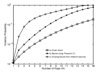
Figure 2: Violation probability of the end-to-end delay bound ($\mu\cdot d=112.5$) in an M/M/1 network as a function of the number of nodes; utilization factor at each node is $\rho=0.7$

To analyse the accuracy of the new probabilistic end-to-end delay bound from Theorem III.1, we compare it with the existing probabilistic bounds from network calculus and results from queueing theory for a network of M/M/1 queues. In an M/M/1 queuing system with one server, both the arrival and the service processes are of Poisson type. The customers arrive at rate $\lambda$ and the server works at rate $\mu$. We denote the utilization factor by $\rho=\lambda/\mu$, and assume for stability that $\rho<1$. The effective bandwidth and effective capacity of the arrival and service processes (Poisson process) are $\lambda\frac{e^{\theta}-1}{\theta}$ and $\mu\frac{1-e^{-\theta}}{\theta}$, respectively, with $\theta^{*}=-\log{\rho}$. We consider a special case of the network from Fig. 1 with $H$ M/M/1 queues connected in series to analyse the accuracy of our end-to-end network calculus delay bound. A Poisson flow with rate $\lambda$ traverses through the entire network. The arrival process at the downstream queue is the departure process of the upstream queue which is again Poissonian. Let each queue in the network be served by a similar service process $S$ with effective capacity $\beta(\theta)$ and let the service processes at all nodes of the network be independent of each other. It is known from queueing theory that the exact distribution of steady state end-to-end delay of the through flow $W(t)$ in a M/M/1 queueing network is given by

$$P\left\{W(t)>d\right\}=\sum_{h=0}^{H-1}\frac{(\mu(1-\rho)d)^{h}}{h!}e^{-\mu(1-\rho)d}$$ (18)

The equation is obtained from an $H$-fold convolution of the (exponential) probability function of delay for a single M/M/1 node, followed by an integration in the limits from d to infinity. The best available end-to-end delay bound of the through flow $W(t)$ in a M/M/1 queueing network from network calculus [1, 11] is given by

$$P\left\{W(t)>d\right\}=\inf_{0\leq\theta\leq\theta^{*}}{\left(\frac{1}{1-e^{-\theta\{\beta(\theta)-\alpha(\theta)\}}}\right)^{H}e^{-\theta\alpha(\theta)d}}$$ (19)

In Fig. 2, we illustrate the violation probability of the delay bounds ($\mu\cdot d=112.5$) from equations (8) and (9) as curve (b) along with the exact results from equation (18) as curve (a) and existing delay bounds from stochastic network calculus using moment generating functions [11, 1] from equation (19) as curve (c) for a fixed utilization factor $\rho=0.7$ at each of the $H$ queues. It can be observed that the new results provide better bounds than the existing bounds and also follow the shape of the exact results from queueing theory.

IV Conclusions

In this paper we used demisubmartingale inequalities to compute end-to-end probabilistic delay and backlog bounds within the framework of network calculus. The tightness of the computed end-to-end probabilistic performance bounds is explored by comparing new bounds with the exact results from queueing theory for a network of M/M/1 queues.

References

- [1] F. Ciucu, “Network calculus delay bounds in queueing networks with exact solutions,” in Proceedings of International Teletraffic Congress (ITC-20), 2007.
- [2] ——, “Exponential supermartingales for evaluating end-to-end backlog bounds,” in Proceedings of Ninth Workshop on Mathematical Performance Modeling and Analysis (MAMA), 2007.
- [3] Y. Jiang, “Network calculus and queueing theory: two sides of one coin,” in Proceedings of the Fourth International ICST Conference on Performance Evaluation Methodologies and Tools, October 20-22, 2009.
- [4] T. Christofides, “Maximal inequalities for n-demimartingales,” Archives of Inequalities and Applications, vol. 1, pp. 397–408, 2003.
- [5] B. P. Rao, “On some maximal inequalities for demisubmartingales and n-demisupermartingales,” Journal of Inequalities in Pure and Applied Mathematics, vol. 8, no. 4, 2007.
- [6] C.-S. Chang, Performance Guarantees in Communication Networks. Springer-Verlag, 2000.
- [7] F. P. Kelly, “Notes on effective bandwidths,” Stochastic Networks: Theory and Applications, vol. Oxford, Royal Statistical Society Lecture Notes Series,, pp. 141–168, 1996.
- [8] S. Shakkottai, A. Kumar, A. Karnik, and A. Anvekar, “TCP performance over end-to-end rate control and stochastic available capacity,” IEEE/ACM Transactions on Networking, vol. 9(4), pp. 377–391, August 2001.
- [9] D. Wu and R. Negi, “Effective capacity: A wireless link model for support of quality of service,” IEEE Transactions on Wireless Communications, vol. 2(4), pp. 630–643, July 2003.
- [10] K. Angrishi and U. Killat, “Analysis of a real-time network using statistical network calculus with effective bandwidth and effective capacity,” in Proceedings of 14. GI/ITG Konferenz Messung, Modellierung und Bewertung von Rechen- und Kommunikationssystemen (MMB 2008), 2008.
- [11] M. Fidler, “An end-to-end probabilistic network calculus with moment generating functions,” in Proceedings of IWQoS, 2006.
- [12] Y. Jiang, “A basic stochastic network calculus,” in Proceedings of ACM SIGCOMM, 2006, pp. 123–134.
- [13] K. Angrishi and U. Killat, “On the threshold for observing approximate invariance of effective bandwidth,” in Proceedings of 2008 International Symposium on Performance Evaluation of Computer and Telecommunication Systems (SPECTS 2008), June 2008.