Fractional oscillator

Abstract

We consider the fractional oscillator being a generalization of the conventional linear oscillator in the framework of fractional calculus. It is interpreted as an ensemble average of ordinary harmonic oscillators governed by stochastic time arrow. The intrinsic absorption of the fractional oscillator results from the full contribution of the harmonic oscillators’ ensemble: these oscillators differs a little from each other in frequency so that each response is compensated by an antiphase response of another harmonic oscillator. This allows to draw a parallel in the dispersion analysis for the media described by the fractional oscillator and the ensemble of ordinary harmonic oscillators with damping. The features of this analysis are discussed.

I Introduction

The harmonic oscillator, given by a linear differential equation of second order with constant coefficients, is a cornerstone of the classical mechanics (see, for example, Landau and Lifshitz (1976); R.P. Feynmann and Sands (1963)). Today this elementary (and fundamental) conception has the widest origin of physical, chemical, engineering applications and needs no introduction. Its success mainly rests on its universality, and its simplicity gives boundless intrinsic capabilities for sweeping generalization. Suffice it to recall the passage from the language of functions in phase space to operators in Hilbert space so that the oscillatory model came strongly in the quantum theory Landau and Lifshitz (1981); Dirac (1982). Therefore no wonder, the fractional calculus has made also an important contribution to this way.

At first the approach had a formal character by changing the second derivative in the harmonic oscillator equation on the derivative of an arbitrary order. After finding out the solutions of such equations their relaxation-oscillation behavior was established Mainardi (1996); Podlubny (1999). The next step was a consideration of the total energy and the phase plane representation for the fractional oscillator B.N. Narahari Achar (2001). To save the dimension of energy, it is necessary to generalize to the notation of momentum, though then the parameter $m$ loses also the ordinary dimension of mass B.N. Narahari Achar (2002). In this case the momentum is expressed in terms of the Caputo-type fractional derivative Podlubny (1999). The fractional oscillator is like a harmonic oscillator subject to a damping. The source of the intrinsic damping is very intriguing. It is not evident from fractional calculus, from the generalization of derivative. The question requires an additional study exceeding the bounds of fractional calculus itself.

Since it is a matter of the fractional integral/derivative with respect to time, the answer to the aforementioned problem should be sought by way of their concrete interpretation. Recently, the probability interpretation of the temporal fractional integral/derivative was suggested in Stanislavsky (2004). There exists a direct connection between stable distributions in probability theory and the fractional calculus. The occurrence of the temporal fractional derivative (or integral) in kinetic equations indicates the subordinated stochastic processes. Their directional process is related to a stochastic process with a stable distribution. The parameter characterizing the stable distribution coincides with the index of the temporal fractional integral/derivative in the corresponding kinetic equation. This means that such a equation describes the evolution of a physical system whose time degree of freedom becomes stochastic Stanislavsky (2003). The purpose of this paper is to expand the interpretation on the fractional oscillator.

The paper is organized as follows. In Sec. II we analyze an ensemble of harmonic oscillators with the stochastic time clock. The new clock (random process) substitutes for the deterministic time clock of the ordinary harmonic oscillator. The nondecreasing random process arises from a self-similar $\alpha$-stable random process of temporal steps. Using properties of the stochastic time clock, we obtain the equation for the fractional oscillator. In the spirit of this approach the fractional oscillator can be considered as an ensemble average of oscillators. Sec. III is devoted to the comparison of dispersion properties of the two media. One of them consists of damped noninteracting harmonic oscillators, whereas another is the fractional oscillator. It turns out that their dispersion characteristics have a lot of common features. We discuss them in detail. Our conclusions are briefly summarized in Sec. IV. Appendix contains calculations for the response of the driven fractional oscillator. They are useful for the dispersion analysis in Sec. III.

II Normal modes

We start our consideration with the classical case of harmonic oscillator. Based on the Hamilton function $\mathcal{H}=(p^{2}+\omega^{2}q^{2})/2$, where $p$ and $q$ are the momentum and the coordinate, respectively, and $\omega$ the proper frequency, the motion equations take the form

$$\partial q/\partial t=\partial\mathcal{H}/\partial p=p,\quad\partial p/\partial t=-\,\partial\mathcal{H}/\partial q=-\omega^{2}.$$ (1)

To multiply the first equation of (1) on $\pm i\omega$ and to add it with the second equation, we arrive at

$$\partial c/\partial t=-i\omega c,\qquad\partial c^{*}/\partial t=i\omega c^{*}\,,$$ (2)

where the complex-conjugate values $c$ and $c^{*}$ satisfy the relations

$$c=(\omega q+ip)/\sqrt{2\omega},\qquad c^{*}=(\omega q-ip)/\sqrt{2\omega}.$$

The solutions of Eqs.(2) can be written as

$$c(t) = c(0)e^{-i\omega t}=\frac{1}{\sqrt{2\omega}}[\omega q(0)+ip(0)]e^{-i\omega t},$$

$$c^{*}(t) = c^{*}(0)e^{i\omega t}=\frac{1}{\sqrt{2\omega}}[\omega q(0)-ip(0)]e^{i\omega t}.$$ (3)

The values $c$ and $c^{*}$ are called else the normal modes of oscillator Landau and Lifshitz (1976). They have a very pictorial presentation in the form of a vector rotating just as, the hand revolves around the clock-face center with the frequency $\omega$.

A physical system of harmonic oscillators coupled to an environment will interact with the environmental degrees of freedom. This leads to a damping of oscillatory motion. If the interaction manifests itself at random fashion, one of possible ways to account for perturbations induced by the environment may be as following. Let us randomize the time clock of the value $c(\tau)$ so that any characteristic time is absent. Assume that the time variable is a sum of random temporal intervals $T_{i}$ on the non-negative semi-axis. If they are independent identically distributed variables belonging to the strict domain of attraction of a $\alpha$-stable distribution ($0<\alpha<1$), their sum has asymptotically (the number of the intervals tends to infinity) the stable distribution with the index $\alpha$. Following the arguments of Stanislavsky (2003); Meerschaert (2004), a new time clock is defined as a continuous limit of the discrete counting process $N_{t}=\max\{n\in{\bf N}:\sum_{i=1}^{n}T_{i}\leq t\}$, where ${\bf N}$ is the set of natural numbers. The time clock becomes the hitting time process $S(t)$. Its basic properties is represented in Meerschaert (2004); A.I. Saichev (1997). The probability density of the process $S(t)$ is written in the form

$$p^{S}(t,\tau)=\frac{1}{2\pi i}\int_{Br}e^{ut-\tau u^{\alpha}}\,u^{\alpha-1}\,du\,,$$ (4)

where $Br$ denotes the Bromwich path. This probability density has a clear physical sense. It describes the probability to be at the internal time $\tau$ on the real time $t$. In the case we determine new normal modes

$$c_{\alpha}(t) = \int_{0}^{\infty}p^{S}(t,\tau)\,c(\tau)\,d\tau\,,$$

$$c^{*}_{\alpha}(t) = \int_{0}^{\infty}p^{S}(t,\tau)\,\,c^{*}(\tau)\,d\tau\,.$$

The direct calculations give

$$q_{\alpha}(t) = [c^{*}_{\alpha}(t)+c_{\alpha}(t)]/\sqrt{2\omega}=q(0)A(t)+\frac{p(0)}{\omega}B(t)\,,$$

$$p_{\alpha}(t) = i[c^{*}_{\alpha}(t)-c_{\alpha}(t)]\sqrt{\omega/2}=p(0)A(t)+\omega q(0)B(t)\,,$$

where

$$A(t) = \int_{0}^{\infty}p^{S}(t,\tau)\,\cos\omega\tau\,d\tau=E_{2\alpha,\,1}(-\omega^{2}t^{2\alpha})\,,$$

$$B(t) = \int_{0}^{\infty}p^{S}(t,\tau)\,\sin\omega\tau\,d\tau=\omega t^{\alpha}E_{2\alpha,\,\alpha+1}(-\omega^{2}t^{2\alpha})\,,$$

and

$$E_{\mu,\,\nu}(z)=\frac{1}{2\pi i}\int_{C}e^{u}\,\frac{u^{\mu-\nu}\,du}{(u^{\mu}-z)}$$

is the two-parameter Mittag-Leffler function Erdélyi (1955). Here it is easy to recognize the classical solutions for $\alpha=1/2$ (exponential function) and $\alpha=1$ (sine and cosine). The functions $A(t)$ and $B(t)$ exhibit clearly the relaxation features for $0<\alpha<1/2$, whereas for $1/2<\alpha<1$ the functions represent a damping oscillatory motion. The latter case just corresponds to the fractional oscillator. In particular the value $A(t)$ satisfies the equation

$$A(t)=A(0)-\frac{\omega^{2}}{\Gamma(2\alpha)}\int^{t}_{0}(t-t^{\prime})^{2\alpha-1}\,A(t^{\prime})\,dt^{\prime}\,,$$

with $A(0)=1$, where $\Gamma(x)$ denotes the gamma function. The appropriate equation can be written also for $B(t)$. It should be recalled here that the power kernel of fractional integral of the order $\alpha$, $0<\alpha<1$ “interpolates” the memory function between the Dirac $\delta$-function (the absence of memory) and step function (complete ideal memory). This means that such memory manifests itself within all the time interval $(0,t)$, but not at each point of time (complete but not ideal memory). Under the ideal complete memory the system “remembers” all its states, and this excites the harmonic oscillations in such a system. The absence of memory causes only the relaxation. The order of fractional integral represents a quantitative measure of memory effects Stanislavsky (2000). In accordance with the theory of memory effects the fractional oscillator contains simultaneously the oscillatory motion and the relaxation.

From the series representation of $E_{\mu,\,\nu}(z)$ we derive the leading asymptotic behavior of the value $A(t)$ and $B(t)$ for $t\to 0$: $\lim_{t\to 0}A(t)=1,\lim_{t\to 0}B(t)=0$. According to Erdélyi (1955), the two-parameter Mittag-Leffler function approaches zero as $z\to\infty$ in the sector of angles $|\arg(-z)|<(1-\mu/2)\pi$, and increases indefinitely as $z\to\infty$ outside of this sector. In our case we can use the following expansion valid on the real negative axis

$$E_{\mu,\,\nu}(z)=-\sum_{n=1}^{N-1}\frac{z^{-n}}{\Gamma(\nu-n\mu)}+O(|z|^{-N}),\quad z\to-\infty\,.$$

Thus, for $0<\alpha<1/2$ and $1/2<\alpha<1$ the value $A(t)$ and $B(t)$ decreases algebraically in time. As distinct from the case of a damping harmonic oscillator, the model describes another damping mechanism, without any external frictional force. The damping of a fractional oscillator is due to internal causes B.N. Narahari Achar (2004). How to explain the attenuated oscillations? This important feature of fractional oscillator has been already noted from time to time in various publications Mainardi (1996); B.N. Narahari Achar (2001, 2002). However, the source of such intrinsic damping remained undecided.

We suggest the following interpretation. The fractional oscillator should be considered as an ensemble average of harmonic oscillators. When all harmonic oscillators are identical, and we set their going in the same phase, their full contribution will be equal to the product of the number of oscillators and the response of one oscillator. This occasion appears if $\alpha=1$. However, if the oscillators differ a little from each other in frequency, even if they start in phase, after a while the oscillators are allocated uniformly up to the clock-face. Each response will have an antiphase response of another oscillator so that the total response of all harmonic oscillators in such a system is compensated. Although each oscillator is conservative (its total energy saves), the system of such oscillators, resulting in the fractional oscillator ($1/2<\alpha<1$), shows a dissipative nature. In this connection it should be pointed out that the similar situation may be observed also in the medium of harmonic oscillators, having a given probability density on frequency (for example, the Lorentz distribution Hecht (2001)). Both these cases are closely connected with each other and have a common ground, though, generally speaking, they describe different physical systems. As has been shown in Riewe (1996, 1997), Lagrangian and Hamiltonian mechanics formulated with fractional derivatives in time can be used for the description of nonconservative forces such as friction. It should be also mentioned an interpretation of fractional oscillator in Tarasov (2004). In this case the Liouville equation is formulated from a fractional analog of the normalization condition for distribution function that can be considered in a fractional phase space. The latter has a fractional dimension as well as the fractional measure. The volume element of the fractional phase space is realized by fractional exterior derivatives. The usual nondissipative systems become dissipative in the fractional phase space. However, the approach is different on ours. It operates with fractional powers of coordinates and momenta. Such fractional systems are nonlinear.

III Dispersion

Now we examine the behavior of the fractional oscillator under the influence of an external force. From above this case corresponds to oscillations in the ensemble of nonidentical harmonic oscillators noninteracting with each other. In the framework of this model the fractional oscillator with the initial conditions $x(0)=0$ and $\dot{x}(0)=0$ is described by the following equation

$$x(t) = -\frac{\omega^{\alpha}_{0}}{\Gamma(\alpha)}\int^{t}_{0}(t-t^{\prime})^{\alpha-1}\,x(t^{\prime})\,dt^{\prime}+$$ (5)

$$+ \frac{1}{\Gamma(\alpha)}\int^{t}_{0}(t-t^{\prime})^{\alpha-1}\,F(t^{\prime})\,dt^{\prime}\,,$$

where it should be kept $1<\alpha<2$, and $F$ is the external force. The dynamic response of the driven fractional oscillator was investigated in B.N. Narahari Achar (2002):

$$x(t)=\int^{t}_{0}F(t^{\prime})\,(t-t^{\prime})^{\alpha-1}\,E_{\alpha,\,\alpha}(-\omega^{\alpha}_{0}(t-t^{\prime})^{\alpha})\,dt^{\prime}\,.$$ (6)

This allows us to define the response for any desired forcing function $F(t)$. The “free” and “forced” oscillations of a fractional oscillator depend on the index $\alpha$. However, in the first case the damping is characterized only by the “natural frequency” $\omega_{0}$, whereas the damping in the case of “forced” oscillations depends also on the driving frequency $\omega$. Each of these cases has a characteristic algebraic tail itself, associated with damping B.N. Narahari Achar (2004).

Let $F(t)$ be periodic, $F(t)=F_{0}\,e^{j\omega t}$. Then the solution of Eq. (5) is determined by taking the inverse Laplace transform

$$x(t)=\frac{1}{2\pi j}\int_{Br}e^{st}\frac{F_{0}\,(s+j\omega)\,ds}{(s^{2}+\omega^{2})\,(s^{\alpha}+\omega_{0}^{\alpha})}\,.$$ (7)

The Bromwich integral (7) can be evaluated in terms of the theory of complex variables. Some particular examples of forcing functions were considered in B.N. Narahari Achar (2002). However, the set turns out to be enough scanty for our aim. The necessary computations with $F(t)=A\sin(\omega t+\phi)$ are fulfilled in Appendix. The phase $\phi$ is constant.

If one waits for a long enough time, the normal mode of this system is damped. Therefore, consider only the forced oscillation. After the substitution of $\bar{x}(t)=x_{0}e^{j\omega t}$ for $x(t)$ in Eq.(5) we obtain

$$x_{0}\,e^{j\omega t} = -\frac{\omega^{\alpha}_{0}}{\Gamma(\alpha)}\int^{t}_{0}(t-t^{\prime})^{\alpha-1}\,x_{0}\,e^{j\omega t^{\prime}}\,dt^{\prime}+$$ (8)

$$+ \frac{1}{\Gamma(\alpha)}\int^{t}_{0}(t-t^{\prime})^{\alpha-1}\,F_{0}\,e^{j\omega t^{\prime}}\,dt^{\prime}\,.$$

It is convenient to change the variable $\omega(t-t^{\prime})=\zeta$ in the integrand. Next we can divide out $\exp(j\omega t)$ from each side of (8) and direct $t$ to infinity. The procedure permits to extract the contribution of steady-state oscillations. Using the table integral Abramowitz and Stegun (1972)

$$\int_{0}^{\infty}z^{\alpha-1}\,e^{-jz}\,dz=\Gamma(\alpha)\,e^{-j\pi\alpha/2}\,,$$

Eq. (8) gives

$$x_{0}=\frac{F_{0}}{[\omega_{0}^{\alpha}+\omega^{\alpha}\exp(j\pi\alpha/2)]}\,.$$ (9)

This result is completely confirmed by a more comprehensive analysis given in Appendix.

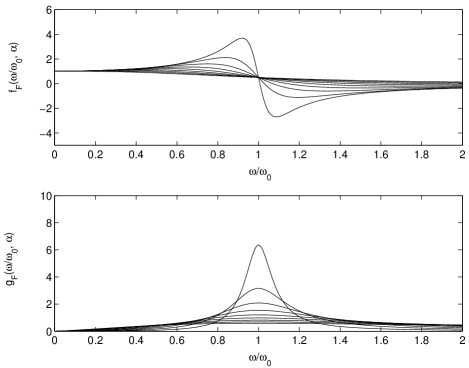
Figure 1: Dispersion dependence of the fractional oscillator in the form of the functions $f_{F}(\omega/\omega_{0},\alpha)$ and $g_{F}(\omega/\omega_{0},\alpha)$ with different values $\alpha$, from 0.1 to 0.9 with the step 0.1.

As is well know, the ensemble behavior of identical noninteracting harmonic oscillators is a basic topic for considering in the classical theory of dispersion. The nonidentity of oscillators is necessary to take into account, for example, for the dispersion analysis of propagating electromagnetic waves into a heated gas, where the spread in molecule velocity values leads to a Doppler shift of the oscillators’ normal frequency with respect to the forced field frequency. Right now let a medium of oscillators be such that results in the fractional oscillator. It interests us the polarizability of such a medium. In this case the permittivity is written as $\epsilon=1+4\pi e^{2}x_{0}/(F_{0}\,m)$, where $e$ is the electron charge. It should be pointed out that in contrast to a simple harmonic oscillator the parameter $m$ does not have the ordinary dimension of mass. However, the generalized momentum $p$ of the fractional oscillator is defined via the Caputo-type fractional derivative of order $\alpha/2$ Podlubny (1999) so that the expression $p^{2}/(2m)$ has the dimension of energy (see details in B.N. Narahari Achar (2002)). The real and imaginary parts of the permittivity take the form

$$\mathrm{Re}\,\epsilon(\omega)=1+\frac{4\pi e^{2}[\omega_{0}^{\alpha}+\omega^{\alpha}\,\cos(\pi\alpha/2)]}{m\,[\omega_{0}^{2\alpha}+\omega^{2\alpha}+2\omega_{0}^{\alpha}\omega^{\alpha}\cos(\pi\alpha/2)]}\,,$$ (10)

$$\mathrm{Im}\,\epsilon(\omega)=-\frac{4\pi e^{2}\omega^{\alpha}\,\sin(\pi\alpha/2)}{m\,[\omega_{0}^{2\alpha}+\omega^{2\alpha}+2\omega_{0}^{\alpha}\omega^{\alpha}\cos(\pi\alpha/2)]}\,.$$ (11)

For $\alpha=2$ we arrive at the Sellmeier’s formula Sellmeier (1871):

$$\epsilon(\omega)=1+4\pi e^{2}N/[m(\omega_{0}^{2}-\omega^{2})]\,,$$

where we include $N$ to account for the number of harmonic oscillators in the medium. In this case the parameter $m$ is really the electron mass. The index $\alpha=2$ corresponds to the classical harmonic oscillator without any damping, and all the oscillators in the ensemble go in the same phase. Therefore, the Sellmeier’s formula contains only the real part of permittivity.

Figure 2: Dispersion dependence in the classical case (ensemble of ordinary harmonic oscillators with damping) with different values $\beta$, from 0.1 to 1.0 with the step 0.1.

We can conduct a clear comparison between the dispersion characteristics of the fractional oscillator and one of an ensemble of classical harmonic oscillators with damping. Normalize the frequency $\omega$ in their permittivity by $\omega_{0}$. In fact the constants (like $e$, $m$ and so on) in $\mathrm{Re}\,\epsilon(\omega)$ and $\mathrm{Im}\,\epsilon(\omega)$ define only a scale. Thus, one can pick out the functional dependence of these permittivities on $\omega/\omega_{0}=z$. Denote $2\gamma/\omega_{0}$ by $\beta$, where $\gamma$ defines the damping in each classical harmonic oscillator. Then we have the following dependences for the fractional oscillator

$$\mathrm{Re}\,\epsilon_{F}(\omega)\quad\to\quad f_{F}(z,\alpha) = \frac{1+z^{\alpha}\,\cos(\pi\alpha/2)}{z^{2\alpha}+2z^{\alpha}\cos(\pi\alpha/2)+1}\,,$$

$$\mathrm{Im}\,\epsilon_{F}(\omega)\quad\to\quad g_{F}(z,\alpha) = \frac{z^{\alpha}\sin(\pi\alpha/2)}{z^{2\alpha}+2z^{\alpha}\cos(\pi\alpha/2)+1}\,,$$

and ones for the classical harmonic oscillators with damping

$$\mathrm{Re}\,\epsilon_{D}(\omega)\quad\to\quad f_{D}(z,\beta) = \frac{1-z^{2}}{(1-z^{2})^{2}+z^{2}\beta^{2}}\,,$$

$$\mathrm{Im}\,\epsilon_{D}(\omega)\quad\to\quad g_{D}(z,\beta) = \frac{z\beta}{(1-z^{2})^{2}+z^{2}\beta^{2}}\,.$$

If the parameter $\beta$ determines the damping value in the harmonic oscillator, the index $\alpha$ just characterizes the same for the fractional oscillator. The extremum values of $f_{D}(z,\beta)$ and $g_{D}(z,\beta)$ decrease with increasing the parameter $\beta$ whereas for $f_{F}(z,\alpha)$ and $g_{F}(z,\alpha)$ vice versa: the extremum values increase with increasing the index $\alpha$, though it should be noted that this index itself belongs only to the interval $1<\alpha\leq 2$. The functions $f_{\cdots}(z)$ and $g_{\cdots}(z)$ are shown on Fig. 2 and Fig. 3.

From the relations (10) and (11) it follows that there is a frequency range, where the absorption is small, and the refraction coefficient increases with frequency (normal dispersion). Moreover, in the frequency range, where the absorption is big, the anomalous dispersion happens to be the case for the refraction coefficient decreasing with frequency. In this connection it should be pointed out that the presence of the normal and anomalous dispersion is typical for such an ensemble of ordinary harmonic oscillators and is well known. However a new fact established here is that the normal and anomalous dispersion is also typical for the medium described as a fractional oscillator.

IV Summary

We have shown that the fractional oscillator can be considered as a model of the harmonic oscillators’ medium. Its stochastic properties accumulate in the index of the fractional integral/derivative with respect to time. The frequency distinction of the oscillators (constituents of the fractional oscillator) from each other is at the bottom of the intrinsic damping for such a system. As a consequence, the dispersion properties of the medium, like the fractional oscillator, is enough similar to the case, when a medium is modeled by an ensemble of harmonic oscillators with damping.

Appendix

We here derive properties of the response function (6) for the forcing function $A\sin(\omega t+\phi)$ directly from its representation as a Laplace inverse integral

$$x(t) = \frac{1}{2\pi j}\int_{Br}e^{st}\,\tilde{x}(s)\,ds=$$

$$= \frac{1}{2\pi j}\int_{Br}e^{st}\frac{A\,(s\cdot\sin\phi+\omega\cdot\cos\phi)\,ds}{(s^{2}+\omega^{2})\,(s^{\alpha}+\omega_{0}^{\alpha})}\,,\quad(\mathrm{A1})$$

where the phase $\phi$ is constant, ${\it Br}$ denotes the Bromwich path, and $1<\alpha\leq~{}2$. By bending the Bromwich path into the equivalent Hankel path (Fig. 3), the response function $x(t)$ can be decomposed into two contributions.

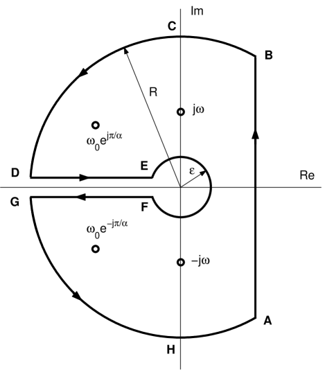
Figure 3: Contour, inside which the function $\tilde{x}(s)$ remains single-valued and analytical all over, with the exception of poles $\pm j\omega$ and $\omega_{0}\exp(\pm j\pi/\alpha)$.

The first contribution arises from the two borders of the cut negative real axis (lines DE and FG):

$$x_{1}(t)=-\frac{1}{2\pi j}\int^{0}_{-\infty}e^{st}\tilde{x}(s)\,ds-\frac{1}{2\pi j}\int^{-\infty}_{0}e^{st}\tilde{x}(s)\,ds.$$

To enter $s=re^{j\pi}$ into the integral taken along the upper border and $s=re^{-j\pi}$ into the integral along the lower border, we get

$$x_{1}(t)=\int_{0}^{\infty}e^{-rt}M_{\alpha}(r)\,dr$$

with

$$M_{\alpha}(r)=\frac{A\,r^{\alpha}\,(\omega\,\cos\phi-r\,\sin\phi)\,\sin\pi\alpha}{\pi\,(r^{2}+\omega^{2})\,(r^{2\alpha}+2r^{\alpha}\omega_{0}^{\alpha}\cos\pi\alpha+\omega_{0}^{2\alpha})}.$$

The second contribution is determined by the Cauchy theorem on residues. The integrand of (A1) has the following poles

$$s=\pm j\omega\qquad\mathrm{and}\qquad s=\omega_{0}e^{\pm j\pi/\alpha}.$$

Calculating the residues of the poles $s=\pm j\omega$, we obtain

$$x_{2}^{\prime}(t)=A\left[\frac{\omega_{0}^{\alpha}\,\sin(\omega t+\phi)+\omega^{\alpha}\sin(\omega t-\pi\alpha/2+\phi)}{\omega_{0}^{2\alpha}+\omega^{2\alpha}+2\omega_{0}^{\alpha}\omega^{\alpha}\cos(\pi\alpha/2)}\right].$$

It remains to define the residues for the two other poles:

$$\left[\frac{e^{st}(s\cdot\sin\phi+\omega\cdot\cos\phi)}{(s^{2}+\omega^{2})\frac{d}{ds}(s^{\alpha}+\omega_{0}^{\alpha})}\right]_{s=\omega_{0}e^{\pm j\pi/\alpha}}=$$

$$= \frac{e^{\omega_{0}t(\cos\pi/\alpha\pm j\sin\pi/\alpha)}[\omega_{0}\,e^{\pm j\pi/\alpha}\,\sin\phi+\omega\cos\phi]}{\alpha\,\omega^{\alpha-1}\,e^{\pm j\pi(\alpha-1)/\alpha}\,[\omega_{0}^{2}e^{\pm 2j\pi/\alpha}+\omega^{2}]}.$$

They lead to

$$x_{2}^{\prime\prime}(t)=\frac{2A\,\exp(\omega_{0}t\cos(\pi/\alpha))\,[C\cos\phi-D\sin\phi]}{\alpha\,\omega^{\alpha-1}\,(\omega_{0}^{4}+\omega^{4}+2\omega_{0}^{2}\omega^{2}\cos(2\pi/\alpha))},$$

where

$$C = \omega[\omega_{0}^{2}\cos(\omega_{0}t\sin(\pi/\alpha)-\pi(1+\alpha)/\alpha)+$$

$$+ \omega^{2}\cos(\omega_{0}t\sin(\pi/\alpha)+\pi(1-\alpha)/\alpha)],$$

$$D = \omega_{0}[\omega_{0}^{2}\cos(\omega_{0}t\sin(\pi/\alpha))+$$

$$+ \omega^{2}\cos(\omega_{0}t\sin(\pi/\alpha)+2\pi/\alpha)].$$

As a result, the response function $x(t)$ takes the form:

$$x(t)=x_{1}(t)+x_{2}^{\prime}(t)+x_{2}^{\prime\prime}(t)\,.$$

Since $\cos(\pi/\alpha)<0$, the term $x_{2}^{\prime\prime}(t)$ describes the relaxation of the normal mode in this system. For $1<\alpha<2$ and all $r$ the denominator of the value $M_{\alpha}(r,\alpha)$ is always positive: $(r^{2\alpha}+2r^{\alpha}\omega_{0}^{\alpha}\cos\pi\alpha+\omega_{0}^{2\alpha})>(r^{\alpha}-\omega^{\alpha}_{0})^{2}\geq 0$, and the term $\sin\pi\alpha$ is always negative. Depending on $\phi$, each of terms $\omega\,\cos\phi$ and $r\,\sin\phi$ may be both positive and negative. However the value $x_{1}(t)$ becomes vanishingly small with $t\to\infty$. The steady-state oscillation in this system is defined only by the term $x_{2}^{\prime}(t)$. The latter can be expressed as $x_{2}^{\prime}(t)=A_{1}\sin(\omega t+\phi-\delta)$, where

$$A_{1} = \frac{A}{[\omega^{2\alpha}+\omega_{0}^{2\alpha}+2\omega^{\alpha}\omega_{0}^{\alpha}\cos(\pi\alpha/2)]^{1/2}},$$

$$\delta = \arctan\left[\frac{\omega^{\alpha}\sin(\pi\alpha/2)}{\omega^{\alpha}\cos(\pi\alpha/2)+\omega_{0}^{\alpha}}\right].$$

To put $\phi=0$ in (A1), we arrive at the results of section 4.3 from B.N. Narahari Achar (2002). It should be also noted that the oscillatory contribution $x_{2}^{\prime\prime}(t)|_{\phi=0}$ has some resemblance with the “free” oscillations of a damped harmonic oscillator and the forced oscillations of a driven damped harmonic oscillator B.N. Narahari Achar (2004).

References

- Landau and Lifshitz (1976) L. Landau and E. Lifshitz, Mechanics : Volume 1 (3rd edition, Butterworth-Heinemann, Boston, MA, 1976).
- R.P. Feynmann and Sands (1963) R.P. Feynmann,R.B. Leighton and M. Sands, The Feynmann Lectures in Physics: Volume 1. (Addison-Wesley, Reading, Massachusetts, 1963).
- Landau and Lifshitz (1981) L. Landau and E. Lifshitz, Quantum Mechanics: Non-Relativistic Theory, Volume 3 (3rd edition, Butterworth-Heinemann, Boston, MA, 1981).
- Dirac (1982) P.A.M. Dirac, Principles of Quantum Mechanics (4th edition, Clarendon Press, Oxford, 1982).
- Mainardi (1996) F. Mainardi, Chaos, Soliton & Fractals 7(9), 1461 (1996).
- Podlubny (1999) I. Podlubny, Fractional Differential Equations (Academic Press, San Diego, 1999).
- B.N. Narahari Achar (2001) B.N. Narahari Achar, J.W. Hanneken,T. Enck,T. Clarke, Physica A287, 361 (2001).
- B.N. Narahari Achar (2002) B.N. Narahari Achar, J.W. Hanneken,T. Clarke, Physica A309, 275 (2002).
- Stanislavsky (2004) A. Stanislavsky, Theor. and Math. Phys. 138(3), 418 (2004).
- Stanislavsky (2003) A. Stanislavsky, Phys. Rev. E67, 021111 (2003).
- Meerschaert (2004) M. M. Meerschaert, H.-P. Scheffler, J. Appl. Probab. 41, 623 (2004).
- A.I. Saichev (1997) A.I. Saichev, G.M. Zaslavsky, Chaos 7, 753 (1997).
- Erdélyi (1955) A. Erdélyi, Higher Transcendental Functions, Volume III (McGraw-Hill, New York, 1955).
- Stanislavsky (2000) A. Stanislavsky, Phys. Rev. E61, 4752 (2000).
- B.N. Narahari Achar (2004) B.N. Narahari Achar, J.W. Hanneken,T. Clarke, Physica A339, 311 (2004).
- Hecht (2001) E. Hecht, Optics (4th edition, Pearson Addison Wesley, Ontario, 2001).
- Riewe (1996) F. Riewe, Phys. Rev. E53, 1890 (1996).
- Riewe (1997) F. Riewe, Phys. Rev. E55, 3581 (1997).
- Tarasov (2004) V.E. Tarasov, Chaos 14, 123 (2004).
- Abramowitz and Stegun (1972) M. Abramowitz and I. Stegun, Handbook of Mathematical Functions (Dover, New York, 1972).
- Sellmeier (1871) Sellmeier, Pogg. Ann. CXLIII, 272 (1871).