Nelkin scaling for the Burgers equation and the role of high-precision calculations

Abstract

Nelkin scaling, the scaling of moments of velocity gradients in terms of the Reynolds number, is an alternative way of obtaining inertial-range information. It is shown numerically and theoretically for the Burgers equation that this procedure works already for Reynolds numbers of the order of 100 (or even lower when combined with a suitable extended self-similarity technique). At moderate Reynolds numbers, for the accurate determination of scaling exponents, it is crucial to use higher than double precision. Similar issues are likely to arise for three-dimensional Navier–Stokes simulations.

Nelkin N90 , showed that the multifractal model of turbulence M74 ; PF83 , implies certain scaling relations for moments of velocity gradients (henceforth gradmoments). According to Nelkin, at high Reynolds numbers, when plotted as a function of the Reynolds number $R$, the $p$th moment of any component $\nabla u$ of the velocity gradient should scale, to leading order, as

$$\langle(\nabla u)^{p}\rangle\sim R^{\chi_{p}}.$$ (1)

The exponents $\chi_{p}$ are expressible in terms of the multifractal structure function exponents $\zeta_{p}$ (cf. N90 or Fbook , Sec. 8.5.6).

By using very highly resolved direct numerical simulation, it has been checked by Schumacher, Sreenivasan and Yakhot that not only is such scaling present (its first verification), but that it is already seen at Reynolds numbers around 200, well below those where structure functions show any inertial-range scaling SSY07 . This is perhaps not so suprising, given that inertial-range scaling is for intermediate asymptotics with two large parameters, the Reynolds number and the ratio of the scale under consideration to the typical dissipation scale, whereas Nelkin scaling just requires a large Reynolds number.

The one-dimensional Burgers equation

$$\partial_{t}u+u\partial_{x}u=\nu\partial_{x}^{2}u;\quad u(x,0)=u_{0}(x),$$ (2)

where $u$ is the velocity and $\nu$ the kinematic viscosity, can can throw light on why gradmoments display good scaling at such moderate Reynolds numbers. Furthermore, it allows analytical determination of all the dominant and subdominant terms in the high-Reynolds number expansion of gradmoments. We note that in a recent paper CFR10 , the Burgers equation was used to illustrate why the extended self-similarity (ESS) technique BCTBMS93 gives improved scaling through the depletion of subdominant corrections.

Heuristically, it is quite simple to show that for the Burgers equation we expect $\chi_{p}=p-1$. Indeed, at high Reynolds numbers, the solutions of (2) display shocks broadened by viscosity over a distance $O(\nu)=O\left(R^{-1}\right)$. Within a shock, the $p$th power of the velocity gradient is $O\left(R^{p}\right)$. Since shocks cover a fraction $O\left(R^{-1}\right)$ of the one-dimensional spatial domain, the stated scaling results. Of course such an argument tells us nothing about subdominant corrections and thus cannot be used to predict at what kind of Reynolds numbers this scaling emerges.

We shall now address these issues more systematically, using simulations and theory. We shall also address a new question: scaling exponents are notoriously known with poor accuracy (cf., e.g., Fbook ); how accurately can we determine such exponents by working with Reynolds number at which there are significant subdominant corrections to scaling? Using recent results of van der Hoeven V09 ; PF07 , we shall show that this requires a subtle tradeoff between Reynolds numbers and precision (number of decimal digits) used in the calculations.

We begin with simulation-based results for the Reynolds number dependence of gradmoments when standard double-precision calculations suffice. We follow here the same strategy as in Ref. CFR10 : we solve the Burgers equation (2) with the initial condition $u_{0}(x)=\sin x$, using a pseudo-spectral method combined with fixed-time-step fourth-order Runge–Kutta time marching and a slaved scheme, known by the acronym ETDRK4 CM02 , for handling the viscous dissipation. The gradmoments of integer order $p$, as a function of the Reynolds number $R\equiv 1/\nu$, are defined as spatial averages over the period $2\pi$:

$$M_{p}(R)\equiv\frac{1}{2\pi}\int_{0}^{2\pi}dx\,\left[\frac{\partial u(x,t)}{\partial x}\right]^{p}.$$ (3)

Gradmoments are calculated for orders $p$ from two to ten and Reynolds numbers $R$ from twenty to one thousand. The number of collocation points $N$ is taken between 8K and 256K where K stands for $2^{10}=1024$; the time step $\delta t$ is between $10^{-5}$ and $10^{-6}$. We checked that the errors on gradmoments stemming from spatial and temporal truncation stay below the level needed for a double-precision calculation. The output is calculated at $t=2$ when the solution of the Burgers equation has a well-developed shock. Since, as explained above, gradmoments are expected to behave asymptotically as $R^{p-1}$ at large $R$, we display them in compensated manner, that is divide them by $R^{p-1}$.

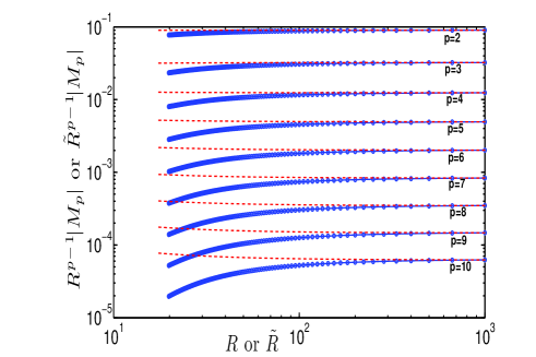
Figure 1: (Colour online) Compensated $p$th-order moments ($p$ from 2 to 10) of velocity gradient ($M_{p}$) versus both $R$ (continuous line with points in blue) and the ESS-type surrogate $\tilde{R}$ (dashed red line).

Figure 1 shows the compensated gradmoments as a function of Reynolds number. Visual inspection shows that the expected flat behavior of the compensated gradmoments sets in around $R=40$ for the lowest order $p=2$ and around $R=300$ for $p=10$. In contrast, inertial-range scaling for structure functions, calculated from the same solution of the Burgers equation, appears clean only around Reynolds numbers of several thousands CFR10 . This discrepancy, of nearly two orders of magnitude, can be made even larger by resorting to a procedure inspired from ESS in which one resorts to a surrogate of the spatial separation, such as the third-order structure function and plots structure functions versus the surrogate. In the case of gradmoments, we observe that the mean energy dissipation is given in terms of the mean square velocity gradient by $\varepsilon=\nu M_{2}=(1/R)M_{2}$. This has a finite positive limit $\varepsilon_{\infty}$ as the Reynolds number tends to infinity. Hence, we can use $\tilde{R}\equiv M_{2}/\varepsilon_{\infty}$ as a (suitably normalized) surrogate of the Reynolds number. This we call ESS-type plotting. The same Fig. 1 also shows this type of plotting. Now, the data look almost completely flat, except for the largest value of $p$ around $\tilde{R}=20$ where the data bend slightly upwards, as revealed by looking at the figure from the side .

Of course, all this has to do with subdominant corrections to scaling and the way they are affected by the ESS-type procedure. We now turn to theoretical interpretations. For this we use the exact solution of the Burgers equation, obtained by employing the Hopf–Cole method H50 ; C51 that transforms the Burgers equation into the heat equation. For the initial condition $u(x,0)=\sin(x)$ this solution reads

$$u(x,t) = -2\nu\partial_{x}\ln\theta(x,t)$$ (4)

$$\theta(x,t) = \int_{0}^{2\pi}\mathrm{e}^{\cos(x-x^{\prime})/(2\nu)}\,G(x^{\prime},t)\,dx^{\prime}.$$ (5)

Here, $G(x^{\prime},t)=\sum_{k=-\infty}^{k=\infty}\mathrm{e}^{\mathrm{i}kx^{\prime}-\nu k^{2}t}$ is the Green’s function for the heat equation in the $2\pi$- periodic case. We want to use this solution to determine the asymptotics of gradmoments for small $\nu$, i.e., large $R$. Using the method of steepest descent, in a way somewhat similar to what is found in Ref. scooped , one can show that, for large $R$ and any integer $p\geq 2$

$$M_{p}(R)=A_{p}R^{p-1}+B_{p}R^{p-2}+C_{p}R^{p-3}+\ldots$$ (6)

The coefficients are given by rather complicated and numerically ill-conditionned integrals.

The expansion (6) and the numerical values of the coefficients can actually be obtained by an alternative semi-numerical procedure, called asymptotic extrapolation, developed by van der Hoeven V09 (see also PF07 for an elementary presentation). Let us now say a few words about this technique, which will also be used below in connection with high-precision spectral calculations. Suppose we have determined numerically with high precision the values of a function $f(n)$ for integers $n$ up to some high value $N$. We wish to obtain from this as many terms as possible in the high-$n$ asymptotic expansion of $f$. Trying to fit the function by a guessed leading asymptotic form with some free parameters, will generally lead to very poor accuracy in such parameters. With some information about the structure of the various terms in the expansion, a better method is to fit an expression containing one or several subdominant corrections (all with some unknown parameters). Lacking such information, asymptotic extrapolation handles the problem by applying to the data a sequence of suitably chosen transformations that successively strip off the dominant and subdominant terms in the expansion for large $n$. At certain stages of such transformations, the processed data allow simple extrapolations, most often by a constant. The transformations are meaningful as long as the successively transformed data is free from conspicuous rounding noise and $n$ has reached a simple asymptotic behavior (e.g. flat). From the extrapolation stages, it then becomes possible (by undoing the transformations made) to obtain the asymptotic expansion of the data (including the values of the various parameters) up to some order which depends on the precision of the data and on the value of $N$. Here, we will denote the transformations by using the notation of Ref. PF07 . Thus, I stands for “inverse”, R for “ratio”, SR for “second ratio” and D for “difference”. The sequence of transformations is chosen through various tests which provide some clue about the asymptotic class in which the data falls.

order$(p)$ $\chi_{p}$ $A_{p}$ $\chi^{(1)}_{p}$ $B_{p}$ $\chi^{(2)}_{p}$ $C_{p}$ 2 0.9999987 +0.09032605 – 0.002 – 0.2290236 – 1.002 +0.2011 3 1.999998 – 0.03245271 1.00001 +0.1736854 0.005 – 0.1325 4 2.999996 +0.01249279 2.00001 – 0.090466 1.0001 +0.08417 5 3.999995 – 0.00498725 3.00001 +0.045622 1.99988 – 0.08209 6 4.999994 +0.00203621 4.00001 – 0.022523 2.99993 +0.06103 7 5.999993 – 0.00084414 5.000008 +0.010955 4.0002 – 0.0398 8 6.999992 +0.0003539 5.999993 – 0.00526 5.002 +0.024 9 7.999994 – 0.0001495 6.99991 +0.0025 6.009 – 0.01 10 9.00001 +0.000063 7.9995 – 0.0012 7.03 +0.03

Table 1: Dominant scaling exponents $\chi_{p}$ and the first two subdominant exponents $\chi_{p}^{(1)}$ and $\chi_{p}^{(2)}$ together with the corresponding coefficients $A_{p}$, $B_{p}$, and $C_{p}$ for the large-$R$ behavior of gradmoments of order $p$, obtained by asymptotic extrapolation processing of a 400-digit precision determination of gradmoments from the Hopf-Cole solution. The theoretical values are $\chi_{p}=p-1$, $\chi_{p}^{(1)}=p-2$, and $\chi_{p}^{(2)}=p-3$.

To apply asymptotic extrapolation to the determination of the coefficients in the high-Reynolds number expansion (6), we calculate the Hopf–Cole solution (4)-(5) and the gradmoments (3) using extreme precision floating point calculations mpfun with 400 decimal digits. This precision guarantees that the only source of errors is lack of simple asymptoticity. The convolution structure of (5) allows the use of fast Fourier transforms, also in very high precision fft , for calculating $\theta$, $u$ and various space derivatives. The Reynolds number $R$ is given all integer values from $18$ to $R_{\rm max}=400$. The processing of the gradmoments for $p$ from 2 to 10 involves typically 15 stages of transformations, the first eight of which are always R - 1, I, D, D, I, D, D, D . From the undoing of the transformations, using the “most asymptotic data points” for determining constants, we obtain the following expansion:

$$M_{p}(R)=A_{p}R^{\chi_{p}}+B_{p}R^{\chi_{P}^{(1)}}+C_{p}R^{\chi_{P}^{(2)}}+\ldots$$ (7)

The results are shown in Table 1. Only those digits of the coefficients that agree when processing the data successively with $R_{\rm max}=200$ and $R_{\rm max}=400$ are shown. It is seen that the scaling exponents for the dominant term $\chi_{p}$ and the first and second subdominant terms, $\chi_{P}^{(1)}$ and $\chi_{P}^{(2)}$ are very close to their theoretical values obtained from (6). The relative discrepancies are in the range $10^{-5}$ – $10^{-6}$ for the dominant exponent and the accuracy degrades for subdominant corrections, as expected.

From the expansion (7) we can readily understand why Nelkin scaling appears at rather moderate Reynolds number: the absolute value of relative correction stemming from the first subdominant term is $R^{-1}|B_{p}/A_{p}|$. For example, it reaches the ten percent level which is easily picked up visually at $R=10|B_{p}/A_{p}|$. Table 2 shows the values of $|B_{p}/A_{p}|$ and we now understand why flat compensated gradmoments are seen in Fig. 1 beyond Reynolds numbers, varying with $p$, from a few tens to a few hundreds. To understand the ESS-type even better scaling, we expand the surrogate $\tilde{R}$ in terms of $R$. From (6) with $p=2$ and noticing that $A_{2}=\varepsilon_{\infty}$, we obtain

$$\tilde{R}=R^{1}+\frac{B_{2}}{A_{2}}R^{0}+O\left(R^{-1}\right).$$ (8)

Eliminating $R$ between (6) and (8), we obtain

$$M_{p}=A_{p}{\tilde{R}}^{p-1}+\tilde{B}_{p}{\tilde{R}}^{p-2}+\ldots;\,{\tilde{B}_{p}}=B_{p}-\frac{(p-1)A_{p}}{A_{2}}B_{2}.$$ (9)

Note that the expansion in terms of the surrogate $\tilde{R}$ has the same structure as (6) and precisely the same dominant-term coefficient $A_{p}$. However the coefficient $\tilde{B}_{p}$ of the first subdominant correction is significantly smaller than $B_{p}$ (in absolute value) and may have a different sign. This explains for example why the graph for the compensated third-order gradmoment in terms of $R$ bends down at the low end while it bends very slightly up in terms of $\tilde{R}$. As a consequence of the reduced subdominant corrections, the asymptotic behavior of gradmoments in the ESS-type representation emerges at Reynolds numbers 5 to 20 times smaller than in the ordinary representation (see Table 2).

order$(p)$ $R_{p}^{\star}=|B_{p}/A_{p}|$ $\tilde{R}_{p}^{\star}=|\tilde{B}_{p}/A_{p}|$ 2 2.5344 0.0 3 5.3520 0.2827 4 7.2414 0.3622 5 9.1477 0.9906 6 11.0613 1.6116 7 12.9785 2.2290 8 14.8980 2.8440 9 16.8222 3.4544 10 19.0604 3.7507

Table 2: Estimates of Reynolds numbers beyond which subdominant corrections become small in the Reynolds number representation (middle column) and in the ESS-type representation (last column).

We should not be carried away and state that good scaling can emerge already at very moderate Reynolds number provided we take the right quantity (here, gradmoments) and the right data processing technique (here, ESS). It all depends on what we call “good scaling”. If we want to obtain scaling exponents with an error not exceeding $10^{-2}$ or $10^{-3}$, a flat looking compensated graph is definitely not enough since this is achieved as soon as the relative error is somewhere below $10^{-1}$. We now address the issue how asymptotic (how large in Reynolds number) and how precise should a spectral calculation be in order to truly give accurate scaling exponents. Of course, the higher the Reynolds number, the lower the relative subdominant corrections will be. But, without enough precision, the simultaneous determination of dominant terms and subdominant corrections, say by asymptotic extrapolation, will be unable to handle more than very few such corrections and thus gives us substantial errors in the final results. In order to be closer to more realistic models such as the multi-dimensional Navier–Stokes equations, in investigating the trade-off between asymptoticity and precision, we refrain from using the exact solution of the Burgers equation and resort to time integration by (pseudo-)spectral technique. We use double and quadruple precision, both combined with asymptotic extrapolation, so as to obtain the most accurate possible parameters. We calculate the scaling exponents $\chi_{4}$ and $\chi_{6}$ of the fourth and the sixth gradmoments, whose theoretical exact values are three and five, respectively. We determine how accurately we can predict these exponents when applying asymptotic extrapolation (which for this purpose is substantially better than the aforementioned ESS technique), using various maximum Reynolds numbers $R_{\rm max}$. In double precision we were able to use three stages and in quadruple precision eight stages of the aforementioned transformations.

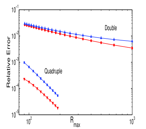
Figure 2: (Color online) Relative error of Nelkin exponents $\chi_{4}$ and $\chi_{6}$ obtained by asymptotic extrapolation from pseudo-spectral calculations up to a maximum Reynolds number $R_{\textrm{max}}$. Upper set of curves: double precision calculations ($\chi_{4}$: red filled circles, $\chi_{6}$: blue filled triangles); lower set of curves: quadruple precision ($\chi_{4}$: red inverted triangles, $\chi_{6}$: blue filled squares).

The maximum wavenumber and the size of the time step are the same as reported at the beginning of the paper. We checked, by further halving of spatial and temporal resolutions, that they contribute negligible errors to the result. Figure 2 shows the relative errors for the two types of precision as function of $R_{\rm max}$. It is striking that, when doubling the precision we can decrease the Reynolds number by about a factor of eleven (from 1000 to 90) and still obtain a substantial decrease (by a factor of 3 to 10) in the relative error. For accurate determination of scaling exponents, increasing the precision is here definitely more efficient than increasing the Reynolds number. It remains to be seen if this result carries over to a much broader class of equations, including multi-dimensional incompressible problems displaying random behavior. Already, we can state that the use of Nelkin scaling to analyze multifractal scaling in simulated 3D turbulent flow should definitely be encouraged, and preferably combined with high precision caculations.

- (1) M. Nelkin, Phys. Rev. A 42, 7226 (1990).
- (2) B. Mandelbrot, J. Fluid Mech. 62, 331 (1974).
- (3) G. Parisi and U. Frisch, in Turbulence and Predictability in Geophysical Fluid Dynamics and Climate Dynamics, edited by M. Ghil, R. Benzi and G. Parisi (North-Holland, Amsterdam, 1985), p. 84.
- (4) U. Frisch, Turbulence — The Legacy of A. N. Kolmogorov, (Cambridge University Press, Cambridge, 1995).
- (5) J. Schumacher, K. R. Sreenivasan and V. Yakhot, New J. Phys. 9, 89 (2007).
- (6) S. Chakraborty, U. Frisch and S. S. Ray, J. Fluid Mech. 649, 275 (2010).
- (7) R. Benzi, S. Ciliberto, R. Tripiccione, C. Baudet, F. Massaioli and S. Succi, Phys. Rev. E 48, R29 (1993).
- (8) J. van der Hoeven, J. Symb. Comput. 44, 1000 (2009).
- (9) W. Pauls, and U. Frisch, J. Stat. Phys. 127, 1095 (2007).
- (10) S. M Cox and P. C. Matthews, J. Comp. Phys. 176, 430 (2002).
- (11) E. Hopf, Comm. Pure Appl. Math. 3, 201 (1950).
- (12) J. D. Cole, Quart. Appl. Math. 9, 225 (1951).
- (13) D. O. Crighton and J. F. Scott, Phil. Trans. Roy. Soc. London 292, 101 (1979).
- (14) D. H. Bailey, “High-Precision Arithmetic in Scientific Computation”, Computing in Science and Engineering, May-June, 2005, pg. 54-61; LBNL-57487. See also http:crd.lbl.govdhbailey
- (15) http:www.kurims.kyoto-u.ac.jpoourafft.html.