Persistent charge and spin currents in a 1D ring with Rashba and Dresselhaus spin-orbit interactions by excitation with a terahertz pulse

Abstract

Persistent, oscillatory charge and spin currents are shown to be driven by a two-component terahertz laser pulse in a one-dimensional mesoscopic ring with Rashba-Dresselhaus spin orbit interactions (SOI) linear in the electron momentum. The characteristic interference effects result from the opposite precession directions imposed on the electron spin by the two SOI couplings. The time dependence of the currents is obtained by solving numerically the equation of motion for the density operator, which is later employed in calculating statistical averages of quantum operators on few electron eigenstates. The parameterization of the problem is done in terms of the SOI coupling constants and of the phase difference between the two laser components. Our results indicate that the amplitude of the oscillations is controlled by the relative strength of the two SOI’s, while their frequency is determined by the difference between the excitation energies of the electron states. Furthermore, the oscillations of the spin current acquire a beating pattern of higher frequency that we associate with the nutation of the electron spin between the quantization axes of the two SOI couplings. This phenomenon disappears at equal SOI strengths, whereby the opposite precessions occur with the same probability.

I Introduction

The reconsideration of the spin-orbit interaction (SOI) in the modern context of spintronic applications, started more than ten years ago, was based on the idea of the possible manipulation of the electron spin by means of an electric field.Datta and Das (1990) While definitive answers to this quest have yet to be reached, the fundamental interest in understanding the effect of SOI on macroscopic phenomenology continues. Associated with the spatial confinement in two-dimensional quantum wellsBychkov and Rashba (1984) (Rashba-R) or with inversion asymmetry in the crystal (Dresselhaus-D) Dresselhaus (1955), SOI is usually considered to be linear in the electron momentum which is coupled to the electron spin through a constant whose magnitude is amenable to outside control. The most important physical aspect associated with the R-D superposition is the effect on the electron spin, which is forced to precess in opposite directions along the quantization directions imposed by the two spin interactions. This phenomenology is embodied by the single particle Hamiltonian,

$$H_{SO}=\frac{\alpha}{\hbar}(\sigma_{x}p_{y}-\sigma_{y}p_{x})+\frac{\beta}{\hbar}(\sigma_{x}p_{x}-\sigma_{y}p_{y})\ ,$$ (1)

which introduces the Rashba and Dresselhaus interaction constants $\alpha$ and $\beta$ which couple the electron momentum $\vec{p}=(p_{x},p_{y})$ with the electron spin represented by the Pauli spin matrices, $\sigma_{x,y}$. The superposition of the Rashba and Dresselhaus terms generates particularly interesting situations when their strengths are equal, such as the cancellation of dephasing for the eigenstate spinors and the ensuing ballistic spin transportSchliemann et al. (2003) or the formation of a persistent spin helix.Bernevig et al. (2006)

In this paper, we investigate the consequences of the Rashba-Dresselhaus superposition on spin and charge currents that are being induced in a quasi-one-dimensional ring by a terahertz laser pulse with a spatial asymmetry. This represents a well known method of current generation which exploits the left-right asymmetry of the electron states that are excited on a time scale that is much shorter than the electron relaxation lifetime in a non-adiabatic process.Gudmundsson et al. (2003); Gylfadottir et al. (2005) In general, by this method, as well as by applying magnetic fields, Moskalets and Büttiker (2003a, b) simultaneous spin and charge current generation occurs.Splettstoesser et al. (2003); Souma and Nikolić (2004); Sheng and Chang (2006) The independent realization of pure spin currents has been addressed in a number of theoretical proposals that considered hybrid structuresSun et al. (2007) or a specific electron configuration (odd numbers of particles).Huang and Shi-Dong (2009) More recently it was shown that a pure spin current can be created non-adiabatically in a ring with Rashba interaction using a radiation pulse with two dipolar components having a spatial dephasing angle $\phi$.nita1 The physical mechanism for spin current generation relies on the interplay between the spin orbit coupling that rotates the electron spin around the ring and the spatial asymmetry of the external excitation, which establish conditions where the charge current disappears, while the spin current reaches a maximum or a minimum level.

This work undertakes the analysis of spin and charge dynamics in the simultaneous presence of Rashba and Dresselhaus SOI, such that two opposite precession directions are imposed on the electron spin. Our numerical results are obtained within an equation-of-motion algorithm for the particle-density operator, that is later involved in calculating the spin and charge currents as statistical averages of the corresponding quantum operators on a few non-interacting electron eigenstates. The internal phase difference $\phi$ between the two laser components along with the coupling strengths of the R and D interactions are the main parameters of the problem. While the latter play a role in determining the magnitude of the effects, the former is shown to influence the spatial distribution of the currents around the ring.

The paper starts by discussing the spectrum of the equilibrium Hamiltonian, in Sec. II, whose eigenstates and eigenvalues are obtained within a direct diagonalization procedure for a small number of electrons. Then, in Sec. III we detail the equation-of-motion algorithm that allows the estimation of the density operator, followed by Sec. IV and V that present our findings. The results are summarized in Sec. VI.

II The Equilibrium Hamiltonian

Our analysis is based on a discrete model of the Hamiltonian that relies on transforming the continuous, quasi-one dimensional ring of radius $r_{0}$ into a sequence of $N$ sites (points) separated by an equivalent lattice constant $a=2\pi r_{0}/N$. In polar coordinates a site of index $n=1,...,N$ has an azimuthal angle $\theta_{n}=2\pi n/N$, the angle difference between two consecutive sites being $\Delta\theta=2\pi/N$. A single particle state that corresponds to an electron of spin $\sigma$ located at point $n$, $|n,\sigma\rangle$, is associated with the creation and annihilation operators $c^{+}_{n,\sigma}$ and $c_{n,\sigma}$. The electrons encased in the ring are described by the Hamiltonian $H_{\rm ring}$ composed out of the kinetic energy $H_{0}$ and the Rashba and Dresselhaus terms, $V_{R}$ and $V_{D}$,

$$H_{\rm ring}=H_{0}+V_{R}+V_{D}\,,$$ (2)

where $V_{R}$ and $V_{D}$ are given by the first and the second term of Eq. (1), respectively. In the representation provided by the single particle states described above, $H_{0}$ is proportional to the hopping energy $V=\hbar^{2}/2m^{*}a^{2}$ ($m^{*}$ being the effective mass of the electron in the host semiconductor material),

$$H_{0}=2V\sum_{n,\sigma}c^{+}_{n,\sigma}c_{n,\sigma}-V\sum_{n,\sigma}c^{+}_{n,\sigma}c_{n+1,\sigma}-V\sum_{n,\sigma}c^{+}_{n,\sigma}c_{n-1,\sigma}\ ,$$ (3)

while the SOI terms $V_{R}$ and $V_{D}$ generate their own energy scales, $V_{\alpha}=\alpha/2a$ and $V_{\beta}=\beta/2a$,

$$V_{R}=-iV_{\alpha}\sum_{n,\sigma,\sigma^{\prime}}\left[{\bf\sigma}_{r}(\theta_{n,n+1})\right]_{\sigma,\sigma^{\prime}}c^{+}_{n\sigma}c_{n+1\sigma^{\prime}}+{\rm H.c.}\,,$$ (4)

and

$$V_{D}=-iV_{\beta}\sum_{n,\sigma,\sigma^{\prime}}\left[{\bf\sigma}_{\theta}(\theta_{n,n+1})\right]^{*}_{\sigma,\sigma^{\prime}}c^{+}_{n\sigma}c_{n+1\sigma^{\prime}}+{\rm H.c.}\,.$$ (5)

For simplicity, it is customary to introduce the azimuthal and radial spin matrices $\sigma_{\theta}$ and $\sigma_{r}$ written in terms of the angle $\theta_{n,n+1}=(\theta_{n}+\theta_{n+1})/2$,

$${\bf\sigma}_{r}(\theta) ={\bf\sigma}_{x}\cos\theta+{\bf\sigma}_{y}\sin\theta\,,$$

$${\bf\sigma}_{\theta}(\theta) =-{\bf\sigma}_{x}\sin\theta+{\bf\sigma}_{y}\cos\theta\,.$$ (6)

In the presence of only one type of SOI, say Rashba, the spectrum of the Hamiltonian, as well as the eigenvalues of the spin operator, can be obtained analytically. The single-particle eigenvectors are also eigenstates of $L_{z}$, the $\hat{z}$ component of the angular momentum, and they are

$$|\Psi_{l+}\rangle=\frac{1}{\sqrt{N}}\sum_{n}e^{il\theta_{n}}\left(\begin{array}[]{c}\cos\theta_{\alpha}\\ -e^{i\theta_{n}}\sin\theta_{\alpha}\end{array}\right)|n\rangle\,$$ (9)

$$|\Psi_{l-}\rangle=\frac{1}{\sqrt{N}}\sum_{n}e^{il\theta_{n}}\left(\begin{array}[]{c}e^{-i\theta_{n}}\sin\theta_{\alpha}\\ \cos\theta_{\alpha}\end{array}\right)|n\rangle\,,$$ (12)

with $l=0,\pm 1,\cdots,\pm(N-1)/2,N/2$ (for N even). Correspondingly, the energy eigenvalues are given by

$$E_{l\pm}=\frac{\epsilon_{l}+\epsilon_{l\pm 1}}{2}+\frac{\epsilon_{l}-\epsilon_{l\pm 1}}{2}\sqrt{1+\tan^{2}2\theta_{\alpha}}\,,$$ (13)

where $\epsilon_{l}=2V-2V\cos(2\pi l/N)\,$ and $\tan 2\theta_{\alpha}=V_{\alpha}/({V\sin(\pi/N)})$. The quantization direction of the spin operator is ${\bf e}_{2\theta_{\alpha}}=\cos 2\theta_{\alpha}{\bf e}_{z}-\sin 2\theta_{\alpha}{\bf e}_{r}$, which is tilted at an angle $2\theta_{\alpha}$ relatively to the $\hat{z}$-axis due to the presence of the of the SOI.Splettstoesser et al. (2003) The eigenstates are spin degenerated and the energies $E_{l\pm}$ correspond to spin eigenvalues of $\pm\hbar/2$ along ${\bf e}_{2\theta_{\alpha}}$. In turn, the Dresselhaus interaction alone determines a similar energy spectrum and eigenstates, but defines another preferential spin orientation direction, ${\bf e}_{2\theta_{\beta}}=\cos 2\theta_{\beta}{\bf e}_{z}+\sin 2\theta_{\beta}{\bf e}_{\theta}^{*}$ where ${\bf e}_{\theta}^{*}=-{\bf e}_{-\theta}$ (${\bf e}_{-\theta}$ is azimuthal direction for the point of angle $-\theta$ of the ring).

When both R and D interactions are present, the diagonalization of the Hamiltonian (2) is possible only by numerical methods and the results are strongly affected by the relative values of the two coupling constants $\alpha$ and $\beta$. The energy spectrum of the equilibrium Hamiltonian, calculated for an even number of sites, $N=20$, is shown in Fig. 1 as a function of $V_{\alpha}$, for different values of $V_{\beta}$.

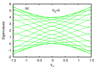
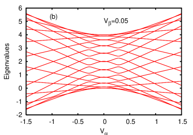
Figure 1: (Color online) The energy spectrum of a ring with SOI versus Rashba energy $V_{\alpha}$. The Dresselhaus energy is $V_{\beta}=0$ in (a) and $V_{\beta}=0.05$ in (b). All energies are given in units of $V=\hbar^{2}/2m^{*}a^{2}$. The spectrum has 40 eigenstates, corresponding to 20 sites $\times$ 2 spin directions. All eigenstates are spin-dengenerated.

All states remain spin degenerate, but other degeneracies are lifted. When $V_{\beta}=0$, as in Fig. 1(a), the spectrum is four fold degenerate for those values of $V_{\alpha}$ that allow the equality $E_{l+}=E_{l^{\prime}-}$ for two different quantum numbers $l$ and $l^{\prime}$. Such degeneracies are lifted when $V_{\beta}\neq 0$ and comparable to $V_{\alpha}$, as shown in Fig. 1(b), where we notice that small energy gaps appear between previously intersecting levels. These gaps give rise to low frequency oscillations of spin and charge currents.

The azimuthal velocity operator $v_{\theta}=r_{0}d\theta/dt=(ir_{0}/\hbar)[H,\theta]$ is evaluated from Eq. (2),

$$v_{\theta}=-i\frac{Va}{\hbar}\sum_{n,\sigma}[c_{n,\sigma}^{\dagger}c_{n+1,\sigma}-c_{n,\sigma}^{\dagger}c_{n-1,\sigma}]$$

$$+2\frac{V_{\alpha}a}{\hbar}\sum_{n,\sigma,\sigma^{\prime}}{\bf\sigma}_{r}(\theta_{n})^{\sigma,\sigma^{\prime}}c_{n,\sigma}^{\dagger}c_{n,\sigma^{\prime}}$$

$$+2\frac{V_{\beta}a}{\hbar}\sum_{n,\sigma,\sigma^{\prime}}{\bf\sigma}^{*}_{\theta}(\theta_{n})^{\sigma,\sigma^{\prime}}c_{n,\sigma}^{\dagger}c_{n,\sigma^{\prime}},$$ (14)

leading to the charge and spin current operators:

$$I = -ev_{\theta}\;,$$

$$I^{s}_{\nu} = \frac{\hbar}{2}\left({\bf\sigma}_{\nu}v_{\theta}+v_{\theta}{\bf\sigma}_{\nu}\right)\;.$$ (15)

In Eq. (15), $\sigma_{\nu}$ is a spin matrix corresponding to the direction ${\bf e}_{\nu}$, which can be any of the Cartesian vectors ${\bf e}_{x}$, ${\bf e}_{y}$, ${\bf e}_{z}$ or ${\bf e}_{2\theta_{\alpha}}$, ${\bf e}_{2\theta_{\beta}}$.

III The Numerical Algorithm

The perturbation Hamiltonian $H_{\rm pulse}$, which represents a laser pulse with two dipolar components of frequencies $\omega_{1}$ and $\omega_{2}$, out of phase with each other by an angle $\phi$, is acting on the few $n_{e}=6$ electrons that occupy the lowest energy eigenstates. In the discrete representation of the ring, we write $H_{\rm pulse}(t)=\sum_{n}H_{\theta}(t)|n\rangle\langle n|$, where the time dependence $H_{\theta}(t)$ at the point $n$ of the ring is:

$$H_{\theta_{n}}(t)=Ae^{-\Gamma t}[\sin(\omega_{1}t)\cos\theta_{n}+\sin(\omega_{2}t)\cos(\theta_{n}+\phi)].$$ (16)

The pulse of amplitude $A$ is applied at time $t=0$ and lasts for a time $t_{f}\sim\Gamma^{-1}$. The density operator $\rho(t)$ satisfies the differential Liouville equation,

$$i\hbar\dot{\rho}(t)=\left[H+H_{\rm pulse}(t),\ \rho(t)\right]\,,$$ (17)

whose solutions are obtained numerically, subject to the initial conditionGylfadottir et al. (2005)

$$\rho(t=0)=\sum_{i=1}^{n_{e}}|\Psi_{i}\rangle\langle\Psi_{i}|\,,$$ (18)

where only the linear superposition of the lowest $n_{e}$ occupied states is considered. For any $t>0$ Eq. (17) generates $\rho(t)$ through the Crank-Nicholson finite difference method Gudmundsson et al. (2003); CN with small time steps $\delta t\ll\Gamma^{-1}$. The expected value of any observable $O$ of the many-body system is then calculated as ${\rm Tr}\left[\rho(t)\hat{O}\right]$, where $\hat{O}$ is the single-particle quantum operator associated to that observable. After the perturbation ceases to act, at time $t>t_{f}$, the system remains in an excited state of constant energy. The time evolution of the expectation values of the system observables is determined by their commutation relation with the Hamiltonian.

In the following calculations the radius of the ring is $r_{0}=14$ nm, which for $N=20$ sites generates a lattice constant $a\approx 4.4$ nm. The effective electron mass in the ring is material dependent, $m^{*}=0.067m_{e}$ for a GaAs or $m^{*}=0.023m_{e}$ for InAs. ($m_{e}$ is the free electron mass.) Table 1 summarizes the various parameters involved in the calculation that pertain to the applied laser pulse (time, frequencies, pulse amplitude $A$) and those that pertain to the physical observables of the system (energy, spin, velocity, charge and spin current $I_{c}$ and $I_{s}$). We also show the correspondence between the SOI parameters $V_{R}$ and $V_{D}$ and Rashba and Dresselhaus constants $\alpha$ and $\beta$ in the two materials.

Physical units
Parameter Unit GaAs InAs Energy ​​ $V\!=\!{\hbar^{2}}/({2m^{*}a^{2}})$ 29.4 meV 85.6 meV Time ​​ ${\hbar}/{V}$ 0.022 ps 0.0076 ps Frequency ​​ ${V}/{\hbar}$ 44.6 THz 130.0 THz Velocity ​​ $aV/\hbar$ 196$\cdot 10^{12}$ nm/s 572$\cdot 10^{12}$ nm/s Charge current ​​ $eaV/\hbar$ ​ 31.5 $\mu$Anm 91.6 $\mu$Anm Spin current ​​ ${aV}/{2}$ ​ 64.6 meVnm 188 meVnm

Table 1: The specific units for energy, time, frequency, charge and spin currents, for GaAs ($m^{*}=0.067m_{e}$) and for InAs ($m^{*}=0.023m_{e}$) quantum rings, used in the numerical calculations. $e$ is the electron charge. The discretization constant is a=4.4 nm and is calculated for a ring of radius $r_{0}=14$ nm with N=20 discrete points. The charge current is defined as $I_{c}=ev$ and spin current is $I_{s}=sv$, $v$ being the velocity and $s$ the average spin angular momentum in units of $\hbar$.

In the numerical calculation we use the pulse frequencies $\omega_{1}=0.0963V/\hbar$ and $\omega_{2}=0.276V/\hbar$, while the attenuation factor and the amplitude are chosen as $\Gamma=4\omega_{1}$ and $A=2.3V$, respectively. The two frequencies are close to the first two Bohr frequencies of the 1D ring calculated in the absence of SOI, $\omega_{21}=0.0978V/\hbar$ and $\omega_{32}=0.284V/\hbar$. A Bohr frequency $\omega_{ij}$ is given by the energy difference $(E_{2i}-E_{2j})/\hbar$, with $E_{2i}$ and $E_{2j}$ being the $2i^{th}$ and $2j^{th}$ eigenvalues of the quantum ring. The factor 2 takes into account the spin degeneracy. The external pulse last about $t_{f}=10/\Gamma$ and is equal to 23$\hbar/V$ dimensionless time units.

According to Table  1, for a GaAs quantum ring, the above values correspond to energies $\hbar\omega_{1}=2.83$ meV, $\hbar\omega_{2}=8.11$ meV, the attenuation factor $\Gamma=4\omega_{1}$, the amplitude $A=67.7$ meV and the external pulse duration of about $t_{f}=0.2$ ps. If an InAs quantum ring is considered, the numerical values associated with the laser pulse are $\hbar\omega_{1}=8.23$ meV, $\hbar\omega_{2}=23.6$ meV, $A=197$ meV and $t_{f}=0.068$ ps.

The strength of the SOI is chosen by using the parameters $V_{\alpha}$ and $V_{\beta}$ in interval $[0,0.08V]$, where $V$ is the energy unit shown in Table 1. A value $V_{\alpha}=0.05V$ corresponds to a Rashba coupling constant $\alpha=12.9$ meVnm in a GaAs quantum ring or $\alpha=37.6$ meVnm in InAs as shown in Table 2.

Values of Rashba and Dresselhaus parameters
Definition GaAs InAs $\alpha=2aV_{\alpha}$ $\alpha$=258.4 meVnm$\cdot V_{\alpha}/V$ $\alpha$=752.7 meVnm$\cdot V_{\alpha}/V$ $\beta=2aV_{\beta}$ $\beta$=258.4 meVnm$\cdot V_{\beta}/V$ $\beta$ =752.7 meVnm$\cdot V_{\beta}/V$

Table 2: The Rashba and Dresselhaus parameters $\alpha$ and $\beta$ for GaAs and InAs quantum rings are expressed in terms of the Rashba and Dresselhaus energies $V_{\alpha}$ and $V_{\beta}$, respectively, in units of $V$. The calculations are done for a ring of radius $r_{0}=14$ nm with N=20 discrete points.

IV charge and spin currents driven by a symmetric pulse

We begin our investigation by analyzing the behavior of charge and spin currents in the presence of an R-D SOI when the ring is excited by a spatially symmetric laser pulse, i. e. $\phi=0$ in Eq. (16). We note that at time $t=0$, the charge current is zero for all strengths of SOI, $V_{\alpha}$ or $V_{\beta}$. Under the effect of the perturbation, left-right electron state imbalance occurs, leading to the establishment of an oscillatory current, as shown in Fig. 2, with period $T$ of thousands of time units $\hbar/V$. There, the intensity $I_{c}(t)$ is plotted for various Rashba couplings when the Dresselhaus coupling assumes two different values, $V_{\beta}=0.03V$ in Fig. 2(a) and Fig. 2(b), and $V_{\beta}=0.05V$ in Fig. 2(c) and Fig. 2(d). The period and amplitude of the current depend on the SOI parameters, reaching a maximum when $V_{\alpha}=V_{\beta}$. The small oscillations of amplitude $\Delta^{\prime}I_{c}<0.012\ eaV/\hbar$ and period $T^{\prime}\approx 16\ \hbar/V$ noticeable in Figs. 2(c) and 2(d) are further investigated in the discussion of the spin currents.

The low frequency of the charge current $\Omega=1/T$ is given by the Bohr frequency corresponding to the occupied states with highest energies in the unperturbed ring, $E_{6}$ and $E_{4}$, such that $\Omega=\omega_{32}/2\pi$. We verified this result for all the SOI strengths used in these calculations. For example, for $V_{\alpha}=0.05$ and $V_{\beta}=0.03$ the first few (relevant) energy levels of the quantum ring are, in the increasing order, $E_{1}=E_{2}=-0.003383,\ E_{3}=E_{4}=0.09131,\ E_{5}=E_{6}=0.09805,\ E_{7}=E_{8}=0.3735,\ E_{9}=E_{10}=0.3850,\ E_{11}=E_{12}=0.8146$. We thus obtain from the energy spectrum $T=2\pi/\omega_{32}\equiv 2\pi/(E_{6}-E_{4})=932$ time units, whereas directly from the numerical results of the time dependent current we get $T=948$. This means that after the perturbation had ceased, the ring remains in an excited state which is a superposition of states with partial population of the energy levels $E_{6}$ and $E_{4}$. The frequency of the oscillations, vs. the Rashba SOI $V_{\alpha}\in[0,0.08V]$, is plotted in Fig. 3, for two values of the Dresselhaus SOI. Both the results obtained directly from the time dependent charge current, and from the Bohr frequency $\omega_{32}$, are shown. The agreement is almost perfect. We find a non-monotonic behavior that is highly dependent on the relative strengths of the two SOI’s, such that for a fixed $V_{\beta}$, the minimum frequency occurs for equal strengths $V_{\alpha}=V_{\beta}$. In this case additional degeneracies exist in the energy spectrum,Schliemann et al. (2003) and therefore when $V_{\alpha}\to V_{\beta}$ all energy gaps tend to shrink. (With our parameters, for equal SOI strengths, we obtain $E_{15}=E_{16}=E_{17}=E_{18}$.)

The fast oscillations of the charge current, which can be seen well in Figs. 2(c-d) can also be explained by the energy spectrum. They are created by transitions between states separated by relatively large energies, like $E_{6}$, $E_{4}$, $E_{2}$ and $E_{8}$ or $E_{10}$. In fact the period of the fast oscillations corresponds to the largest energy gap in this series, $T^{\prime}=2\pi/(E_{10}-E_{2})\approx 16\ \hbar/V$.

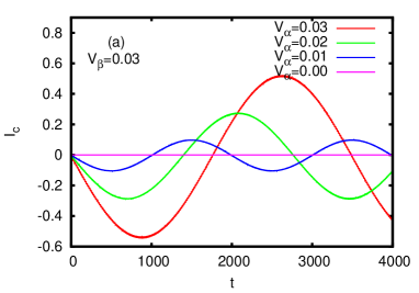
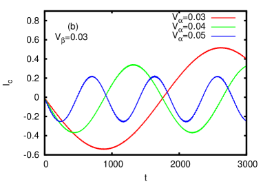
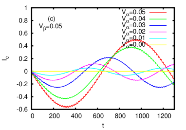
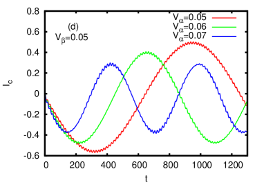
Figure 2: (Color online) Charge currents $I_{c}(t)$ in the presence of both Rashba and Dresselhaus SOI. $V_{\beta}=0.03$ in (a) and (b) and $V_{\beta}=0.05$ in (c) and (d). $V_{\alpha}$ is written in the figures. The minimum frequency $\Omega_{min}=1/T_{max}$ and the maximum amplitude of the oscillations in time, $\Delta I_{c}$, are obtained for $V_{\alpha}=V_{\beta}$. $\Omega_{min}=0.00028$ for $V_{\alpha}=V_{\beta}=0.03V$ and $\Omega_{min}=0.0008$ for $V_{\alpha}=V_{\beta}=0.05V$. The ring and pulse parameters are described in the text. $I_{c}$ is expressed in $eaV/\hbar$ and time in $\hbar/V$ units.

.

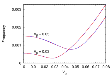
Figure 3: (Color online) The frequency of the long oscillations of the charge current are plotted as functions of the Rashba energy $V_{\alpha}$ for two values of the Dresselhaus coupling $V_{\beta}=0.03V$ and $V_{\beta}=0.05V$ respectively. The continuous lines are obtained from the time dependent output data shown in Fig. 2. The dotted lines show the results for the Bohr frequency $\omega_{32}/2\pi\equiv(E_{6}-E_{4})/(2\pi)$ (see text). The minimum frequency is obtained for $V_{\alpha}=V_{\beta}$. The frequency unit is $V/\hbar$ and $V_{\alpha}$ is in units of V.

Under the same circumstances we study the time variation of the spin current associated to the spin projection along the $\hat{z}$-direction, $I_{z}(t)$, for various values of the SOI interactions. In this instance, the oscillatory behavior associated with charge displacement is complicated by a a beating pattern with nodal points of zero oscillation, as seen in Figs. 4(a) and (c). Zooming in near the nodal points, we obtain Fig. 4(b) and 4(d), where it is readily observable that, as it passes through a nodal point, the spin current phase changes by $\pi$. As before, the amplitude of the oscillations depends on the two SOI interactions and their ratio, while the period of the fast oscillations $T^{\prime}$ seems quite insensitive to this aspect. The period of the fast oscillations is $T^{\prime}\approx 8\ \hbar/V$ or slightly more for all examples shown in Figs. 4(a-b), while the amplitude varies from zero, at nodal points, to about $0.1\ aV/2$. The period $T^{\prime}$ of the spin current is actually half of the period of the fast oscillations of the charge current (also denoted by $T^{\prime}$ in the analysis of that current, and found there $\approx 16$ time units). The reason is that the spin precesses relatively to two principal axes, independently. The axes are tilted at different angles $2\theta_{\alpha}$ and $2\theta_{\beta}$, due to the Rashba and Dresselhaus SOI, respectively. The frequency of the spin current is thus roughly the double of that for the charge current, because of the two spin modes.nita2 For $V_{\alpha}=V_{\beta}$ the spin oscillations cancel each other and the spin current vanishes, as seen in Figs. 4(a) and (c). For $V_{\alpha}\neq V_{\beta}$ the spin current actually has an aperiodic time evolution, observable in the same mentioned figures. So we cannot really speak about a rigorous periodicity of the spin current, and consequently of the charge currents as well.

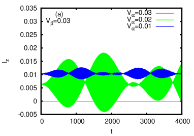
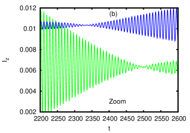
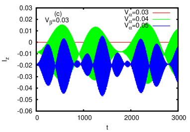
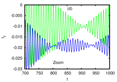
Figure 4: (Color online) The time variation of the spin current $I_{z}(t)$ in the presence of Rashba and Dresselhaus SOI. The Dresselhaus energy is $V_{\beta}=0.03$ in (a) and (b). The Rashba energy is $V_{\alpha}=0.01,0.02,0.03$ in (a) and $V_{\alpha}=0.03,0.04,0.05$ in (b). For $V_{\alpha}=V_{\beta}$ the spin current is zero. For $V_{\alpha}\neq V_{\beta}$ there are spin current oscillations. Figures (c) and (d) present a magnified view of (a) and (b) respectively. (Spin current unit is $aV/2$ and time unit is $\hbar/V$.)

We interpret the beating pattern of the spin current oscillations by a nutation motion of the electron spin between the two quantization directions ${\bf e}_{2\theta_{\alpha}}$ and ${\bf e}_{2\theta_{\beta}}$ imposed by the SOI couplings that force the electron spin precession in opposite directions. When only one type of the SOI, say Rashba, is present, ${\bf e}_{2\theta_{\alpha}}$ becomes a good quantization axis for spin. The corresponding spin current $I_{2\theta_{\alpha}}$ commutes with the equilibrium Hamiltonian and consequently, remains constant in time as a conserved observable. When the SOI parameters are not equal, the principal spin axes have different angles $2\theta_{\alpha}\neq 2\theta_{\beta}$ and the electron spin executes rapid oscillations between them.

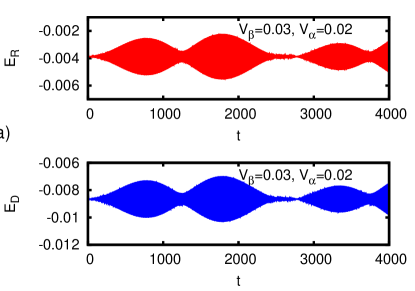
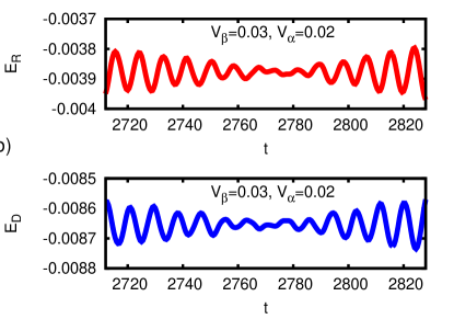
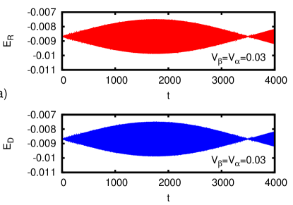
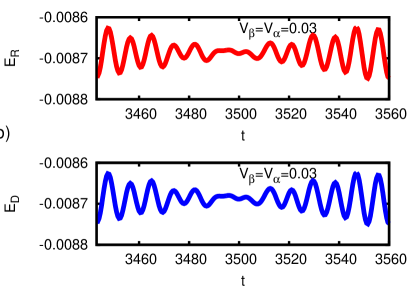
Figure 5: (Color online) The out of phase oscillations of the Rashba and Dresselhaus potential energies, $E_{R}(t)$ and $E_{D}(t)$. $V_{\beta}=0.03V$ and $V_{\alpha}=0.02V$, (a) for the complete time interval, and (b) zoomed into a small time interval. The energy unit is V and time unit is $\hbar/V$.

Figure 6: (Color online) The in phase oscillations of the Rashba and Dresselhaus potential energies, $E_{R}(t)$ and $E_{D}(t)$, for $V_{\beta}=V_{\alpha}=0.03V$, (a) for the complete time interval, and (b) zoomed into a small time interval. The energy unit is V and time unit is $\hbar/V$.

Another perspective on this phenomenon is revealed by plots of the time oscillation of the SOI energy, $E_{R}$ and $E_{D}$, defined as the expected values of the potential energies $V_{R}$ and $V_{D}$ given by Eqs. (4-5). Figs. 6(a) and 6(b) display $E_{R}(t)$ and $E_{D}(t)$ for different values of SOI, while in 6(a) and 6(b) the same value $V_{\alpha}=V_{\beta}$ is used. It appears that an exchange between Rashba and Dresselhaus potential energies occurs with the same oscillation period as the $I_{z}$ beat oscillations. The orbital motion of the electron is thus accompanied by vibrations of the spin orientation between these two directions that give rise to out of phase oscillations of Rashba and Dresselhaus energy. At equal SOI parameters, $V_{\alpha}=V_{\beta}$, the two potential energies reach the same value and oscillate in-phase. Since the precession of the electron spin around the two preferential directions or the Rashba and Dresselhaus SOI’s occurs with equal amplitudes in opposite directions, the spin current vanishes.

V Charge and Spin currents driven by an asymmetric pulse

The time evolution of the electronic states in the quantum ring excited by an asymmetric pulse is asymmetric is discussed next. This involves the full form of Eq. (16), with $\phi\neq 0$. In this case, we are interested in establishing the geometric effect that the dephasing angle $\phi$, varied in fixed steps $\phi=0$, $\pi/6$, $2\pi/6$, $\cdots$, $11\pi/6$, has on the charge and spin currents. To better focus on this aspect, the Rashba and Dresselhaus interactions are fixed at values $V_{\alpha}=0.02V$ and $V_{\beta}=0.03V$, respectively. In our analysis, two dynamic regimes are considered, delimited by the lifetime of the perturbation, $t_{f}$, one occurring for $t<t_{f}$, and the other one for $t>t_{f}$ when the persistent oscillatory behavior is established.

In Fig. 7(a) the charge current $I_{c}(t,\phi)$ is shown to evolve under the effect of the two-component laser pulse between $0<t<t_{f}$, from zero at $t=0$ to non-zero values at $t=t_{f}$, for several angles $\phi$. The largest currents occur for dephasing angles $\phi=4\pi/6$ and $8\pi/6$, whereas the minima occur for $\phi=0$ and $\pi$. A similar pattern is seen in Fig. 7(b), where the dependence of the instantaneous charge current at a given time $I_{c}(t,\phi)$ is depicted for various angles $\phi$. A maximum variation is noticeable at $\phi=\pi/2$ and $3\pi/2$ only for $t=5\hbar/V$ and $t=8\hbar/V$, while for larger times, such as at $t=20\hbar/V$ for instance, the maximum variation of the induced current $|I_{c}(t)|$ is realized for dephasing angles $\phi=4\pi/6$ and $8\pi/6$ as already seen in Fig. 7(a).

After the radiation pulse vanishes, i. e. for $t>t_{f}\simeq 25\hbar/V$, the charge current oscillates with a period $T\simeq 2783\hbar/V$, as shown in Fig. 7(c), where now the time covers one complete period. The amplitude of the oscillations is strongly affected by the value of the dephasing angle. For the dephasing angles $\phi=0$, $\pi/6$ and $11\pi/6$ the time dependence of the charge current has the shape of the function $-\sin(2\pi t/T)$, and will be called here type A oscillations. For the angles $\phi=3\pi/6$, $4\pi/6$, $8\pi/6$, and $9\pi/6$ the oscillations look like $\sin(2\pi t/T)$ and will be called type B oscillations. Type B are shifted from type A by half a period, $T/2$. Type A oscillations of much smaller amplitudes are also seen in Fig. 7(c) for $\phi=6\pi/6$, and also for $\phi=2\pi/6$ and $10\pi/6$. The latter two are actually asymmetric and in transition from type A to type B. For $\phi=5\pi/6$ and $7\pi/6$ again small amplitudes are obtained, this time for oscillations of type B. The amplitude of the current, defined as $\Delta I_{c}=|I_{c}(T/4)-I_{c}(3T/4)|$, changes with $\phi$ as shown in Fig. 7(d). As the angle $\phi$ is varied, the two types of oscillations alternate. This result defines four critical angles $\phi=\phi_{c1,c2,c3,c4}$ that correspond to a crossover from type A to type B. Their numerical values obtained by the interpolation of the presented curves are: $0.35\pi$, $0.85\pi$, $1.15\pi$, and $1.65\pi$, respectively. At the A to B crossover, ı. e. at the critical angles $\phi_{c1,\dots,c4}$, the oscillations of the charge current vanish, as shown in Fig. 7(d). This means that, by tuning the value of the dephasing angle of the external pulse such that $\phi=\phi_{c1,\dots,c4}$ the ring can be excited into a final state that supports a non-zero charge current with zero amplitude, although the current operator $I_{c}$ is a nonconservative observable in the presence of both Rashba and Dresselhaus interactions. The time average of the charge oscillations, defined as $\langle I_{c}\rangle_{t}=(I_{c}(T/4)+I_{c}(3T/4))/2$, is also shown in Fig. 7(d) as function of $\phi$. We note that, for type A oscillations, $\langle I_{c}\rangle_{t}=0$ for angle $\phi=\phi_{m}=0$ and $\pi$, and acquires its maximum and minimum values of $\pm 0.4$ at the angle $\phi=\phi_{M}=0.6\pi$ and $\phi=\phi_{-M}=1.4\pi$, for B type oscillations. This suggests that, by tuning the dephasing angle $\phi$, both the type of charge current oscillations, as well as their time average can be modified.

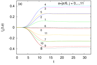
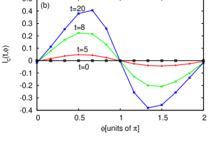
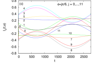
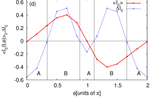
Figure 7: (Color online) (a) The charge current $I_{c}(t,\phi)$ as function of time during the radiation pulse for $t\in[0,33]$, for different angles $\phi=j\pi/6$ between the two dipoles. The integer $j=1,2,...,11$ is indicated near each curve. In (b) we show the charge current as a function of $\phi$ at several moments shown in the graph, $t=0,5,8$ and $20$. (c) The time evolution of the current over a full period of the oscillation $T\approx 2783$. The angles $\phi$ are the same as in (a). (d) The average charge current $\langle I_{c}\rangle_{t}$ and the amplitude $\Delta I_{c}$ are shown versus the angle $\phi$. The time average is $\langle I_{c}\rangle_{t}=[I_{c}(T/4)+I_{c}(3T/4)]/2$ and the amplitude is $\Delta I_{c}=I_{c}(T/4)-I_{c}(3T/4)$. The intervals of type A and type B oscillations are indicated. The SOI parameters are $V_{\alpha}=0.02V$ and $V_{\beta}=0.03V$. Time physical units are $\hbar/V$ for the time and $eaV/\hbar$ for the current.

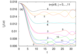
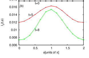
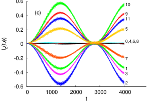
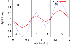
Figure 8: (Color online) (a) The spin current $I_{z}(t,\phi)$ during the pulse, for $t\in[0,33]$ in (a) for the same series of angles between the dipoles as in Fig. 7(a). In (b) we plot the spin current vs. the angle $\phi$ at several moments, t=0, 5 and 8. (c) The spin current along the $z$ direction within a complete period $T$. The spin currents have long oscillations with period $T\simeq 2783$ and short oscillations with $T^{\prime}\simeq 8$. The integers $j=1,2,...,11$ near the curve correspond to the angles $\phi=j\pi/6$. In (d) we summarize the results by showing the time average of the spin current $\langle I_{z}\rangle_{t}=(I_{z}(T/2)+I_{z}(T))/2$ and its amplitude $\Delta I_{z}=I_{z}(T/2)-I_{z}(T)$ versus the dephasing angle $\phi$ and we indicate oscillations of type A and type B. The SOI parameters are $V_{\alpha}=0.02V$ and $V_{\beta}=0.03V$. Time unit is $\hbar/V$ and the unit for the spin current is $Va/2$.

In a parallel analysis, we present the time evolution of the spin current in Fig. 8. At time $t=0$, the ring is found in the ground state, which has a permanent spin current $I_{z}(t=0)=0.01760Va/2$. Along the SOI principal axes the spin currents are $I_{2\theta_{\alpha}}(t=0)=0.01775Va/2$ and $I_{2\theta_{\beta}}(t=0)=0.01793Va/2$, respectively. After the onset of the laser pulse, for $t<t_{f}$, the spin current changes non-adiabatically, as displayed in Fig. 8(a) for different dephasing angles $\phi$. In this time interval the magnitude of $I_{z}(t)$ decreases in time, the variation $I_{z}(0)-I_{z}(t)$ being a function of $\phi$. Snapshots of $I_{z}(t,\phi)$ recorded at times $t=0,\ 5\hbar/V,\ 8\hbar/V$ are plotted against the dephasing angle $\phi$ in Fig. 8(b). We note that the smallest variation $I_{z}(0)-I_{z}(t)$ occurs for $\phi=0$ and the largest for $\phi=2\pi$.

After the radiation pulse vanishes, i. e. for $t>t_{f}$, the quantum ring enters the oscillatory regime. Similar to the charge current, the spin current has an oscillatory behavior with period $T\simeq 2783\hbar/V$ shown in Fig. 8(c) where we plot $I_{z}(t)$. The amplitude $\Delta I_{z}$ varies from $-0.6Va/2$ to $0.6Va/2$ when the angle $\phi$ of the external pulse is changed from $2\pi/6$ to $10\pi/6$, as seen in Fig. 8(c). In addition to the big oscillation with period $T$ and large amplitude $\Delta I_{z}\in[-0.6:0.6]Va/2$, the spin current presents an overlapping pattern of small oscillations, with smaller period $T^{\prime}=8\hbar/V$ and smaller amplitude $\Delta^{\prime}I_{z}\simeq 0.03Va/2$. A similar analysis can be done for the spin currents in the directions $2\theta_{\alpha}$ and $2\theta_{\beta}$ (not shown in the figures). The small and fast beating oscillation have a lower amplitude than for $I_{z}$. In the present example the oscillations of $I_{2\theta_{\beta}}$ are slightly larger than those of $I_{2\theta_{\alpha}}$ because $V_{\beta}>V_{\alpha}$.

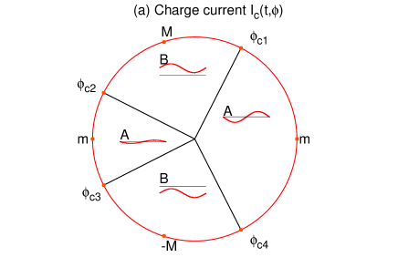
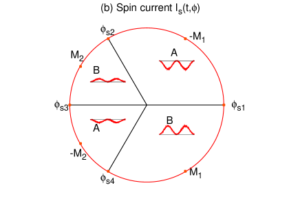
Figure 9: (Color online) By varying the dephasing angle $\phi$ of the external pulse different types of charge and spin current oscillations are induced in the quantum ring. (a) The charge current has oscillations in time of type A or B. For type A the average current vanishes for the angles $\phi$ between the dipolar components of the radiation pulse marked with $m$. Type B oscillations occur for $\phi\in[\phi_{c1},\phi_{c2}]$ and $\phi\in[\phi_{c3},\phi_{c4}]$. In this case the average current has maximum positive and minimum negative amplitudes for the angles marked with M and -M. At the critical points $\phi_{c1\cdots 4}$ the charge current is constant in time. (b) The oscillations of the spin current are also classified as type A and B. For type A the averages current has minimum and negative values at the point $-M_{1}$ and $-M_{2}$. For type B it has maximum positive values at the points $M_{2}$ and $M_{1}$. The two types of oscillations, A and B, for both $I_{c}$ and $I_{s}$, are in antiphase, respectively.

The analysis of Fig. 8(c) indicates that there are two type of spin current oscillations. For the angle $\phi=2\pi/6$, $3\pi/6$, $\pi/6$ and $7\pi/6$, the analytic behavior for the time dependence of spin current is fitted by a function $\cos(2\pi t/T)$ that defines type A oscillations. For values of the dephasing angle $\phi=5\pi/6$, $11\pi/6$, $9\pi/6$ and $10\pi/6$ , the analytic representation is $-\cos(2\pi t/T)$. This defines type B oscillations that are $T/2$ dephased from type A. For certain values of $\phi$ the amplitude of the broad oscillations of $I_{z}$, $\Delta I_{z}$, become comparable with the amplitude of the fast and small oscillations of amplitude $\Delta^{\prime}I_{z}$. This happens for $\phi=0$, $\pi$, $2\pi/3$ and $4\pi/3$ in Fig. 8(c). In the later case the large oscillations with long period $T$ vanish and the remaining feature is the beating pattern with nodal points already shown in Fig. 4.

The amplitude of the big oscillation, $\Delta I_{z}=I_{z}(T/2)-I_{z}(T)$, is found to be negative for type A and positive for type B oscillations, which is shown in Fig. 8(d). By varying $\phi$ the spin current switches between A and B type oscillations at four values of the dephasing angle, denoted as $\phi_{s1,\dots,s4}$. As shown in Fig. 8(d) the critical values are 0, $2\pi/3$, $\pi$, and $4\pi/3$ ($j=0,4,6,8$). The time average of the spin current, $\langle I_{z}\rangle_{t}=(I_{z}(T/2)+I_{z}(T))/2$, is also plotted in Fig. 8(c). When $\phi$ changes $\langle I_{z}\rangle_{t}$ varies between locally minimum and negative value for $\phi=\phi_{-M1}=2\pi/6$ and for $\phi=\phi_{-M2}=7\pi/6$ reached within type $A$ oscillations, and locally maximum positive values for $\phi=\phi_{M2}=5\pi/6$ and $\phi=\phi_{M1}=10\pi/6$ within type B oscillations. These results indicate that the type of oscillations performed by the spin current induced by the two-component radiation pulse, as well as the average spin currents, can be selected by changing the dephasing angle $\phi$.

The behavior of the spin current along the directions ${\bf e}_{2\theta_{\alpha}}$ and ${\bf e}_{2\theta_{\beta}}$ is qualitatively similar to the spin current $I_{z}(t)$, having the same periodicity and beating structure. The amplitude of the fast oscillations is however smaller than for $I_{z}(t)$.

In deriving these results we ignored the inhomogeneity of the electron distribution around the ring, which is known to appear in the simultaneous presence of the Rashba and Dresselhaus terms.Sheng and Chang (2006); nowak Underlying this choice is the fact that the charge deformation in a realistic ring is small, and even questionable for a narrow two-dimensional ring, unless placed in an external magnetic field.nowak Moreover, when the electron-electron interaction is considered for more than two electrons, the charge fluctuation is flattened out due to screening.daday For our one-dimensional ring model the electron density has minima at polar angles $\pi/4$ and $5\pi/4$ and maxima at $3\pi/4$ and $7\pi/4$. Therefore, since the circular symmetry is intrinsically broken in the ground state, a radiation pulse with only one dipolar component would, in principle, be sufficient to induce persistent oscillations of the charge and spin currents.nita2

VI Summary and conclusions

We investigate the interference effect generated by the simultaneous presence of the Rashba and Dresselhaus spin-orbit interactions on charge and spin currents induced non-adiabatically in a quasi-one-dimensional ring by a two-component radiation (laser) pulse. Our numerical results are obtained for a system of few non-interacting electrons through a direct calculation that involves the exact, time-dependent solution of the density operator. The main finding of this work is that the oscillatory behavior of the charge and spin currents is realized at a frequency equal to the difference between two excited energy states (Bohr frequencies).

By varying the dephasing angle $\phi$ between the two dipoles of the external pulse, different types of charge and spin current oscillations are induced in the ring. The general features are summarized in Fig. 9(a) and Fig. 9(b), respectively. By changing the internal dephasing angle $\phi$ in the two intervals $[\phi_{c4},\phi_{c1}]$ and $[\phi_{c2},\phi_{c3}]$ the oscillations of the charge current in time are qualitatively like  $-\sin(2\pi t/T)$, i. e. the oscillations of type A indicated in Fig. 9(a). The average current is zero (i. e minimum) at the angles indicated by the letter ”m” in Fig. 9(a), which are $\phi=0$ and $\phi=\pi$. For $\phi\in[\phi_{c1},\phi_{c2}]$ and $\phi\in[\phi_{c3},\phi_{c4}]$ the charge current oscillates in time (qualitatively) like the function $\sin(2\pi t/T)$, which are oscillations of type B, phase shifted with $T/2$ relatively to the ones of type A. The time average has positive maximum and negative minimum values at the angles marked with $M$ and $-M$ in Fig. 9(a). When the angle $\phi$ has the critical values $\phi_{c1,\dots,c4}$ a crossover between the two types of oscillations occurs, and the charge current is constant in time.

The spin current has also such oscillations in time. When the angle $\phi$ is in the two intervals $[\phi_{s1},\phi_{s2}]$ and $[\phi_{s3},\phi_{s4}]$ the induced spin current oscillates in time as $\cos(2\pi t/T)$, indicated as oscillations of type A in Fig. 9(b). The time average of the spin current has the minimum (negative) values at the points marked as $-M_{1}$ and $-M_{2}$. For $\phi\in[\phi_{s2},\phi_{s3}]$ and $\phi\in[\phi_{s4},\phi_{s1}]$ the spin current oscillate in time as  $-\cos(2\pi t/T)$, marked as oscillations of type B in Fig. 9(b), and dephased with T/2 relatively to type A. Their maximum positive values occur at the angles marked with $M_{2}$ and $M_{1}$. These are wide oscillations with long period $T$ and large amplitude.

In addition, the spin current has also tiny oscillations with a much smaller period $T^{\prime}$ and amplitude $\Delta^{\prime}$. These high-frequency oscillations are caused by the nutation of the electron spin between the spin axes imposed by the R and D couplings. When the angle $\phi$ is close to the critical points $\phi_{s1,\dots,s4}$ a crossover occurs between type A and type B oscillations (or vice versa) of the spin current. For these values of the angle $\phi$ the amplitude of the wide oscillations of $I_{z}$ ($\Delta$) decreases and becomes comparable to the amplitude of fast oscillations ($\Delta^{\prime}$). The spin current oscillations reduce to a beating pattern, while the wide oscillation with long period $T$ vanishes.

After the original excitation disappears the system sustains two persistent types of oscillations of the charge and spin currents, which we classified as type A and type B. The two types of oscillations are in antiphase. Transitions between these modes can be controlled by varying the dephasing angle between the two components of the radiation pulse, an idea with potential applications in the spin-based information technology.