Three-dimensional Hydrodynamic
Instabilities in Stellar Core Collapses

Abstract

A spherically symmetric hydrodynamic stellar core collapse under gravity is time-dependent and may become unstable once disturbed. Subsequent nonlinear evolutions of such growth of hydrodynamic instabilities may lead to various physical consequences. Specifically for a homologously collapse of stellar core characterized by a polytropic exponent $\Gamma=4/3$, we examine oscillations and/or instabilities of three-dimensional (3D) general polytropic perturbations. Being incompressible, the radial component of vorticity perturbation always grows unstably during the same homologous core collapse. For compressible 3D perturbations, the polytropic index $\gamma$ of perturbations can differ from $\Gamma=4/3$ of the general polytropic hydrodynamic background flow, where the background specific entropy is conserved along streamlines and can vary in radius and time. Our model formulation here is more general than previous ones. The Brunt$-$V$\ddot{\rm a}$is$\ddot{\rm a}$l$\ddot{\rm a}$ buoyancy frequency ${\cal N}$ does not vanish, allowing the existence of internal gravity g${}^{-}-$modes and/or g${}^{+}-$modes, related to the sign of ${\cal N}^{2}$ respectively. Eigenvalues and eigenfunctions of various oscillatory and unstable perturbation modes are computed given asymptotic boundary conditions. As studied in several specialized cases of Goldreich & Weber and of Cao & Lou, we further confirm that acoustic p$-$modes and surface f$-$modes remain stable in the current more general situations. In comparison, g${}^{-}-$modes and sufficiently high radial order g${}^{+}-$modes are unstable, leading to inevitable convective motions within the collapsing stellar interior; meanwhile sufficiently low radial order g${}^{+}-$modes remain stably trapped in the collapsing core. Unstable growths of 3D g$-$mode disturbances are governed dominantly by the angular momentum conservation and modified by the gas pressure restoring force. We note in particular that unstable temporal growths of 3D vortical perturbations exist even when the specific entropy distribution becomes uniform and $\gamma=\Gamma=4/3$. Conceptually, unstable g$-$modes might bear conceivable physical consequences on supernova explosions, the initial kicks of nascent proto-neutron stars (PNSs) of as high as $\sim 200-500\hbox{ km s}^{-1}$ up to $\;\lower 4.0pt\hbox{${\buildrel\displaystyle>\over{\sim}}$}\;1000\hbox{ km s}^{-1}$ and break-ups of the collapsing core, while unstable growths of vortical perturbations can lead to fast spins of compact objects, 3D vortical convections inside the collapsing core for possible magnetohydrodynamic (MHD) dynamo actions on seed magnetic fields, and the generation of Rossby waves further stimulated by gravitational wave emissions.

1 Introduction

Over past several decades, considerable theoretical and numerical efforts have been devoted to examine (in)stability properties of core collapsing stars before or around the emergence of supernova (SN) rebound shock expanding inside a massive progenitor star (e.g. Goldreich & Weber 1980 – GW hereafter; Goldreich, Lai & Sahrling 1996; Lai 2000; Lai & Goldreich 2000; Blondin, Mezzacappa & DeMarino 2003; Murphy, Burrows & Heger 2004; Lou & Wang 2006, 2007; Burrows et al. 2006, 2007; Lou & Cao 2008; Cao & Lou 2009, 2010; Lou & Wang 2011). A homologously collapsing relativistically hot or degenerate gas sphere was first studied by GW to describe the pre-SN stellar core collapse process, in which the gas pressure $p$ and the mass density $\rho$ obey the conventional polytropic equation of state (EoS) $p=\kappa\rho^{\Gamma}$ where $\Gamma=4/3$ and $\kappa$ are two global constants. In physically realistic situations, both parameters $\Gamma$ and $\kappa$ do not remain constant in space and time due to multiple complicated nuclear processes including various neutrino productions, electron captures etc. for the inner $\sim 1.5M_{\odot}$ iron core collapse according to numerical simulation results (e.g. Van Riper & Lattimer 1981; Burrows & Lattimer 1983; Bethe 1990; Hix et al. 2003). A decrease of the homologous stellar core mass may occur (e.g. Bethe 1990). One may then introduce a mean value $<\Gamma>$ as a pressure weighted spatial average. Meanwhile, a few numerical simulations (e.g. Van Riper & Lattimer 1981; Burrows & Lattimer 1983, 1986; Bethe 1990) show that the specific entropy closely related to $\kappa$ does not vary much in time before the pre-shock stage for a pre-SN, and that the mean value $<\Gamma>$ does not deviate from $4/3$ significantly. General relativistic simulations of Dimmelmeier et al. (2008) appear to confirm the near constancy of $\Gamma$ before the emergence of a bounce shock. Moreover, other numerical simulations (e.g. Bruenn 1989a,b) show that the homologous solution for a stellar core collapse represents a fair first-order approximation. Based upon their homologous core collapse solution, GW further carried out a vorticity-free (i.e. a potential flow) three-dimensional (3D) perturbation analysis and claimed that no instabilities occur for such a dynamic stellar core collapse. Polytropic homologous core collapse solutions for $\Gamma<4/3$ have been later explored by Yahil (1983), and 3D perturbation analysis on these generalized solutions later show that for $\Gamma>1.09$ no instabilities arise (e.g. Lai 2000). We note that all these previous 3D perturbation analyses are actually restricted to acoustic p$-$modes as the Brunt$-$V$\ddot{\rm a}$is$\ddot{\rm a}$l$\ddot{\rm a}$ buoyancy frequency ${\cal N}$ vanishes in these model considerations.

Lou & Bai (2011) presented 3D isothermal perturbations in a self-similar isothermal nonlinear dynamic flow. Such 3D perturbations can be cast into a self-similar form to describe various possible 3D dynamic flow structures and configurations. In fact, this isothermal requirement can be relaxed to allow a more general EoS. Lou & Cao (2008) generalized the self-similar or homologous core collapse solutions of $\Gamma=4/3$ for a more general EoS by allowing a variable $\kappa$ that is actually conserved along streamlines such that $\kappa$ becomes an arbitrary function of the independent self-similar variable which is a proper combination of radius $r$ and time $t$; in other words, GW solutions only represent a special subclass for a conventional polytropic relativistically hot or degenerate gas of $\Gamma=4/3$. Numerical simulations for the internal structure of massive progenitor stars and SN explosions (e.g. Bethe et al. 1979; Bruenn 1985; 1989a, b; Woosley, Langer & Weaver 1993; Woosley, Heger & Weaver 2002) seem to indicate that the specific entropy distribution is generally non-uniform and can vary in space and time.

The stellar iron core collapse, subsequent core bounce and shock emergence are complicated processes and involve several essential aspects of physics including various nuclear reactions, neutrino trapping and escape, energy transport, a sophisticated EoS (both at mass densities below and above normal nuclear density of $\sim 2-3\times 10^{14}\hbox{g cm}^{-3}$), general relativistic effects, variations of characteristic physical parameters and so forth (e.g. Bethe 1990 and references therein). Hydrodynamic instabilities due to several relevant physical processes may appear before or during an SN explosion due to the core collapse of a massive progenitor star (e.g., with a mass $M\;\lower 4.0pt\hbox{${\buildrel\displaystyle>\over{\sim}}$}\;10M_{\odot}$). The development of numerical simulation models and codes (mostly spherically symmetric) over five decades has reached various levels of sophistication. Within the past decade in particular, the majority of simulation work has been multi-dimensional in nature. Recent multi-dimensional numerical simulations show that the growth of 2D and 3D disturbances can be significant and may be essential for the neutrino convection/heating and thus the viability of the subsequent SN explosion (e.g. Dessart et al. 2006; Buras et al. 2006a, b; Iwakami et al. 2008; Nordhaus et al. 2010b). Among others, hydrodynamics (the so-called advective-acoustic “standing accretion shock instability” or SASI, see e.g. Foglizzo 2001; Blondin et al. 2003; Blondin & Mezzacappa 2006) and neutrino-driven convections can lead to 2D instabilities. For example, it has been shown that the $l=1$ mode is dominant and that a bipolar sloshing of the standing shock wave occurs, with strong pulsational expansions and contractions along the symmetry axis. These numerical simulations indicate that the growth of initial perturbations seems to occur only after the nascent PNS is formed (e.g. Dessart et al. 2006; Nordhaus et al. 2010b). In this context, contributions of the pre-bounce core collapse process to the growth of unstable perturbations should not be ignored, which could perhaps affect an SN explosion directly or indirectly (e.g., by adjusting the process of neutrino convection and heating). In numerical simulation studies, it is not a trivial task to introduce self-consistent dynamic fluctuations during the process of core collapse phase; this is because in many situations, such perturbation solutions are not known or available a priori. Often, one has to rely on the inevitable imprecision of numerical codes as initial perturbations. This might miss unstable growth effects of some perturbations during the earlier stellar core collapse phase. For example, Buras et al (2006a, b) studied partly effects of the pre-bounce perturbations and rotations by numerical simulations. They add arbitrary core collapse density perturbations, which would be more of acoustic nature, and find that the PNS convection starts slightly earlier, though nothing changes significantly. In the numerical simulation of Iwakami et al. (2008) where small initial radial velocity perturbations are added, a linear growth phase before the SN explosion is in fact observed, during which the amplitudes of the initial perturbations grow nearly exponentially with time $t$. Though they start their simulations from a post-bounce time, the stellar core is still contracting before the final explosion; this observation may still be traced back to implicate possible g$-$mode and/or vortical instabilities during the early stellar core collapse phase even when the shock has not yet emerged. It deems important to treat unstable perturbations with care during the early core collapse process. This paper is devoted to analyze the growth of 3D unstable perturbations during the process of the stellar core collapse before the core bounce.

In order to catch dynamic perturbation properties, we shall adopt in this paper a very much simplified yet still fairly challenging general polytropic EoS to describe a nonlinear core collapse of spherical symmetry and perform 3D general polytropic perturbation (in)stability analysis. Bethe (1990 and extensive references therein) reviewed the similarity core collapse solutions (GW; Yahil & Lattimer 1982; Yahil 1983) which appear to capture several gross features of numerical simulations. Though limited, such analytic and semi-analytic approaches may reveal certain physical aspects more transparently. Likewise, we hope to derive useful hydrodynamic instability properties for a more general class of homologous core collapses and offer valuable physical insights for further multi-dimensional numerical simulation explorations, in spite of several simplifications and approximations involved in our hydrodynamic model formulation. Among others, such non-spherical effects have also been shown highly relevant to gravitational wave emissions during a violent dynamic stellar collapse involving rotating iron cores (e.g. Saen & Shapiro 1978; Dimmelmeier et al. 2008 and extensive references therein). In numerical simulations, it is also valuable to introduce self-consistent perturbation solutions to initiate well-controlled code testing and to clearly identify physical effects.

The 3D polytropic perturbation analysis for $\gamma=4/3$ on these generalized dynamic collapse solutions by Cao & Lou (2009) with a self-similar evolution/distribution of specific entropy show that qualitatively analogous to stellar oscillations about a static star (e.g. Cowling 1941; Cox 1976; Unno et al. 1979), all kinds of perturbation modes (i.e. acoustic p$-$modes, surface f$-$modes and internal gravity g$-$modes) exist, and instabilities can always develop for certain g$-$modes of sufficiently high radial orders. Cao & Lou (2009) demonstrated that the sign of the Brunt$-$V$\ddot{\rm a}$is$\ddot{\rm a}$l$\ddot{\rm a}$ buoyancy frequency squared ${\cal N}^{2}$, which determines the existence of internal g$-$modes in static stellar models, still holds the key for g$-$modes during the self-similar dynamic evolution phase of a collapsing stellar core. Prior perturbation analyses (e.g. GW; Lai 2000; Lai & Goldreich 2000) were based on the collapsing stellar core model with a globally constant specific entropy distribution, for which the gas flow is conventional polytropic and thus ${\cal N}^{2}=0$, such that all g$-$modes are actually suppressed. Therefore, GW analysis only indicates that acoustic p$-$modes and f$-$modes remain stable in a homologous core collapse. Cao & Lou (2009) further confirmed the stability of p$-$modes and f$-$modes with a variable specific entropy evolution/distribution, but they clearly found that all g${}^{-}-$modes and sufficiently high-order g${}^{+}-$modes are unstable during the core collapse of a massive progenitor star. They estimated and proposed that the instability of the lowest radial order $l=1$ g$-$modes can lead to initial kicks of nascent PNSs with speeds of as high as $\sim 200-500\hbox{ km s}^{-1}$ up to $\;\lower 4.0pt\hbox{${\buildrel\displaystyle>\over{\sim}}$}\;1000\hbox{ km s}^{-1}$ (e.g., Scheck et al. 2004, 2006, Nordhaus et al. 2010a, and references therein). Our PNS kick proposal differs from several other suggested mechanisms. For example, SN explosions in binary systems do not produce high enough kick speeds of PNSs (e.g. Lai et al. 2001). Hydrodynamic simulations for anisotropic mass ejection in an SN explosion have produced fairly low recoil velocities of NS (e.g. Janka & Müller 1994) or started from the assumption that a dipolar asymmetry was present in the pre-collapse iron core leading to a large anisotropy of an SN explosion (e.g. Burrows & Hayes 1996). Nevertheless, the physical origin of such pre-collpase fluctuations is not at all clear for the moment (e.g. Murphy et al. 2004). In fact, various kinds of hydrodynamic instabilities might be responsible for a large-scale deformation of the ejecta and globally aspherical SN explosions. Our unstable $l=1$ g$-$modes during core collapse appear to be plausible for generating such dipolar asymmetry in envelope mass ejection. Note also that perturbation analysis of Chandrasekhar (1961) found the highest growth rates for the $l=1,m=0$ mode for thermal convection within a gravitating fluid sphere.

Adopting the stellar collapse model with a constant specific entropy distribution as in GW, Cao & Lou (2010) considered non-isentropic perturbations with a perturbation polytropic index $\gamma\neq\Gamma=4/3$, for which ${\cal N}^{2}$ does not vanish. In a complementary perspective, the results of Cao & Lou (2010) also reveal instabilities of g${}^{-}-$modes and sufficiently high radial order g${}^{+}-$modes.

To reveal behaviours of g$-$modes for the most general cases, we perform here a 3D perturbation analysis of the collapsing stellar core model by allowing not only the self-similar profile of the specific entropy to be arbitrary, but also the perturbation polytropic exponent $\gamma$ being different from $\Gamma=4/3$ of the dynamic background. Under such more general conditions, the Brunt$-$V$\ddot{\rm a}$is$\ddot{\rm a}$l$\ddot{\rm a}$ buoyancy frequency ${\cal N}$ does not vanish in general and g$-$modes exist as expected. The instability properties of g$-$modes are further explored in this paper, and several possible processes which may happen during a pre-SN stellar core collapse are discussed in reference to these instabilities, including the formation of PNSs and initial kicks of nascent PNSs. In addition, we also search for the mechanism of unstable g$-$modes in the core collapsing process of a massive progenitor star, and it is shown that the amplification of g$-$mode perturbations which are mainly convective are mostly due to the conservation of angular momentum.

More importantly, 3D vorticity perturbations in a dynamically collapsing stellar core with a uniform specific entropy distribution and perturbation polytropic exponent $\gamma=\Gamma=4/3$ are in fact unstable. In the more general case of a variable specific entropy evolution/distribution and a perturbation polytropic exponent $\gamma\neq\Gamma=4/3$, the radial component of vorticity perturbation always grows in an unstable manner. The growth of such vorticity perturbations may lead to fast spins of collapsing stellar cores, vortical convections or circulations, as well as nonlinear Rossby waves over a spinning PNS and so forth.

After an introduction of background information and our research motivation in Section 1, we present a hydrodynamic description for the dynamics of spherical self-similar general polytropic stellar core collapse in Section 2. Formalism for 3D general polytropic perturbations in a spherically symmetric dynamic stellar collapse is shown in Section 3. Model analysis and results are described in Section 4. Conclusions are summarized in Section 5. Details of specific mathematical analysis can be found in Appendices A through D for the convenience of reference.

2 Homologous stellar core collapse of polytropic gas

Fully nonlinear hydrodynamic partial differential equations (PDEs) include conservations of momentum and mass, the Poisson equation relating the gravitational potential $\Phi$ and the mass density $\rho$, and a general polytropic EoS (i.e. specific entropy conservation along streamlines); these PDEs are

$$\frac{\partial\mathbf{u}}{\partial t}+(\mathbf{u}\cdot\nabla)\mathbf{u}=-\frac{\nabla p}{\rho}-\nabla\Phi\ ,$$ (1)

$$\frac{\partial\rho}{\partial t}+\nabla\cdot(\rho\mathbf{u})=0\ ,$$ (2)

$$\nabla^{2}\Phi=4\pi G\rho\ ,$$ (3)

$$\bigg{(}\frac{\partial}{\partial t}+\mathbf{u}\cdot\nabla\bigg{)}\ln\bigg{(}\frac{p}{\rho^{\Gamma}}\bigg{)}=0\ ,$$ (4)

where $\mathbf{u}(\mathbf{r},\ t)$, $p(\mathbf{r},\ t)$, $\rho(\mathbf{r},\ t)$ and $\Phi(\mathbf{r},\ t)$ are the bulk flow velocity, gas pressure, mass density and gravitational potential of a self-gravitating flow, respectively, the gradient operator $\nabla$ is in terms of the 3D position vector $\mathbf{r}$, $G=6.67\times 10^{-8}\ {\rm cm}^{3}\ {\rm g}^{-1}{\rm s}^{-2}$ is the gravitational constant, and $\Gamma=4/3$ is the polytropic exponent for a dominant Fermi gas consisting of relativistic particles (mainly electrons, positrons, and neutrinos in a radiation field). For a progenitor stellar core collapse prior to an SN explosion, the stellar core temperature is of order of several MeV or higher. This is indeed very hot in terms of gas temperature, i.e. $\sim 10^{10}-10^{11}$ K. Nevertheless, from the perspective of central electron chemical potential $\mu_{e}\sim 300$ MeV and the neutrino chemical potential $\mu_{\nu}\sim 200$ MeV, the core temperature of a few MeV is fairly low and the relativistic Fermi-Dirac gas remains highly degenerate (e.g. Bethe 1990).

It is known that nonlinear hydrodynamic PDEs (1)$-$(4) remain invariant under the following time reversal operation,

$$t\rightarrow-t,\qquad\mathbf{u}\rightarrow\mathbf{-u},\quad\ \rho\rightarrow\rho,\quad\ p\rightarrow p,\quad\ \Phi\rightarrow\Phi\ ,$$ (5)

such that a time-dependent hydrodynamic solution for a stellar core collapse may be reversed to effectively describe a dynamic outflow or expansion.

In reference to Cao & Lou (2009), we first derive in the following self-similar dynamic collapse solutions of spherical symmetry and introduce the time-dependent spatial scale factor $a(t)$ as

$$a(t)=\rho_{c}(t)^{-1/3}\bigg{(}\frac{\kappa_{c}}{\pi G}\bigg{)}^{1/2}\ ,$$ (6)

where the time-dependent $\rho_{c}(t)$ and the constant coefficient $\kappa_{c}$ represent respectively the values of mass density $\rho$ and specific entropy parameter $\kappa$ at the centre (hence a subscript _c) of a massive spherical progenitor star. With this spatial length scale factor $a(t)$ defined by equation (6), the vector radius $\mathbf{r}$ is replaced by a dimensionless vector radius $\mathbf{x}=\mathbf{r}/a(t)$. From now on, we use $\mathbf{u_{0}}(r,\ t)$, $\rho_{0}(r,\ t)$, $p_{0}(r,\ t)$ and $\Phi_{0}(r,\ t)$ to denote the dimensional unperturbed radial bulk flow velocity, mass density, gas pressure and gravitational potential for the self-similar dynamic solution of the general polytropic flow background. The spherically symmetric background flow takes the form of

$$\mathbf{u_{0}}(r,\ t)=\dot{a}\mathbf{x}\ ,$$ (7)

$$\rho_{0}(r,\ t)=\bigg{(}\frac{\kappa_{c}}{\pi G}\bigg{)}^{3/2}a^{-3}f^{3}(x)\ ,$$ (8)

$$p_{0}(r,\ t)=\kappa\rho_{0}^{4/3}=\frac{\kappa_{c}^{3}}{(\pi G)^{2}}a^{-4}g(x)f^{4}(x)\ ,$$ (9)

$$\Phi_{0}(r,\ t)=\frac{4}{3}\bigg{(}\frac{\kappa_{c}^{3}}{\pi G}\bigg{)}^{1/2}a^{-1}\psi(x)\ ,$$ (10)

where $\kappa(r,\ t)$ bears the form of $\kappa_{c}g(x)$ with a constant $\kappa_{c}$, and $f(x)$ is a newly introduced reduced function of only $x$ directly related the mass density $\rho_{0}(r,\ t)$ of the dynamic background flow and is to be determined by hydrodynamic equations [see nonlinear ODE (15) below]. Substituting expressions (7)$-$(10) for the dynamic background flow into nonlinear hydrodynamic PDEs (1)$-$(4) by imposing spherical symmetry and without further approximations, we derive a set of coupled nonlinear ordinary differential equations (ODEs). It can be readily confirmed that PDEs (2) and (4) are automatically satisfied, and $g(x)$ is allowed to take on a fairly arbitrary form, which gives the freedom to specify the self-similar evolution/distribution of the specific entropy. For the $g(x)=1$ case, we would have the special subcase of a conventional polytropic relativistically hot or degenerate gas with a global constant specific entropy parameter $\kappa=\kappa_{c}$ as studied previously by GW. With a more general $g(x)$ profile for the specific entropy distribution/evolution, nonlinear PDE (1) of momentum conservation leads to

$$-\bigg{(}\frac{\pi G}{\kappa_{c}^{3}}\bigg{)}^{1/2}a^{2}\ddot{a}=\frac{1}{x}\bigg{[}\frac{1}{f^{3}}\frac{\mbox{d}}{\mbox{d}x}(gf^{4})+\frac{4}{3}\frac{\mbox{d}\psi}{\mbox{d}x}\bigg{]}\ ,$$ (11)

where the left-hand side (LHS) depends on time $t$ only while the right-hand side (RHS) depends only on the independent self-similar variable $x\equiv|\mathbf{x}|=r/a(t)$. We should then require both sides equal to a constant separation parameter $4\lambda/3$, yielding the two separate nonlinear ODEs below

$$-\bigg{(}\frac{\pi G}{\kappa_{c}^{3}}\bigg{)}^{1/2}a^{2}\ddot{a}=\frac{4\lambda}{3}\ ,$$ (12)

$$\frac{\mbox{d}\psi}{\mbox{d}x}=\lambda x-\frac{3}{4f^{3}}\frac{\mbox{d}}{\mbox{d}x}(gf^{4})\ .$$ (13)

ODE (12) can be solved analytically to obtain an explicit temporal expression for the radial length scale factor $a(t)$ necessary for defining the independent self-similar variable $x\equiv|\mathbf{x}|=r/a(t)$ by equation (6) and the radial flow $\mathbf{u_{0}}=\dot{a}\mathbf{x}$ of the dynamic background by equation (7). The solution for the spatial scale factor $a(t)$ from ODE (12) for a homologous stellar core collapse (GW) is simply

$$a(t)=(6\lambda)^{1/3}\bigg{(}\frac{\kappa_{c}^{3}}{\pi G}\bigg{)}^{1/6}t^{2/3}\ ,$$ (14)

where a positive separation constant $\lambda>0$ is a physical requirement. Substituting ODE (13) into Poisson equation (3) that relates the gravitational potential $\Phi$ and the mass density $\rho$, we readily attain a nonlinear ODE of $f(x)$ below

$$\frac{1}{x^{2}}\frac{\mbox{d}}{\mbox{d}x}\bigg{[}\frac{x^{2}}{f^{3}}\frac{\mbox{d}}{\mbox{d}x}(gf^{4})\bigg{]}+4f^{3}=4\lambda\ .$$ (15)

We can prescribe substantially different yet plausible forms of $g(x)$ for specific entropy evolution/distribution and numerically integrate nonlinear ODE (15) with proper boundary conditions using the standard fourth-order Runge-Kutta integration scheme (e.g. Press et al. 1986). For instance, it is possible to impose $f(x_{b})=0$ at the moving boundary $x=x_{b}$ for a homologously collapsing stellar core (e.g. a PNS). Once $f(x)$ is solved satisfying the specified boundary conditions, the mass density $\rho_{0}(r,\ t)$ and other physical variables characterizing the general polytropic dynamic background flow can all be derived accordingly [see eqns (7)$-$(10) and (13)].

For the $\lambda=0$ case, nonlinear ODE (15) reduces to the general polytropic Lane-Emden equation (e.g. Eddington 1926; Chandrasekhar 1939; Cao & Lou 2009). As an additional necessary check of the consistency, ODE (15) reduces to equation (16) of GW precisely as expected for $g(x)=1$. We would set $f(0)=1$ as a consistent normalization for nonlinear ODE (15). In general, Cao & Lou (2009) require $g^{\prime}(0)=0$ and $f^{\prime}(0)=0$ for a finite sound speed at the centre, where the prime ^′ indicates the first derivative in terms of the independent self-similar variable $x$. As first shown by GW and confirmed by Lou & Cao (2008), there exists a maximum acceptable value of $\lambda>0$, denoted by $\lambda_{M}$, for $f(x)$ to vanish at a finite value of $x=x_{b}$; in the parameter regime of $\lambda>\lambda_{M}$, $f(x)$ would have a minimum but will not reach zero within the semi-infinite interval $0\leq x<+\infty$. By numerical computations for the special case of $g(x)=1$, this range for sensible $\lambda$ values is $0\leq\lambda\leq\lambda_{M}=0.00654376$.

In our scenario, we identify this $x_{b}$ as the contracting surface of the inner homologously collapsing stellar core and the enclosed core mass within $x_{b}$ remains unchanged. In earlier numerical simulations on the stellar iron core collapse (e.g. van Riper & Lattimer 1981; Burrows & Lattimer 1983; Dimmelmeier et al. 2008), both $\Gamma$ and $\kappa$ change in a complicated manner along mass parcels as dictated by several nuclear processes. One consequence of variable $\kappa$ and $\Gamma$ in a collapsing star is that the mass of the inner homologously collapsing core decreases during the stellar core collapse to form a PNS with a mass of no more than $\sim 0.5M_{\odot}$ at the end of collapse. In our dynamic model of stellar core collapse, $\Gamma=4/3$ does not change and $\kappa(r,\ t)=\kappa_{c}g(x)$ evolves in a self-similar yet fairly arbitrary manner. As the enclosed mass $M$ within $x_{b}$ remains constant, we cannot directly model the gradual mass reduction of the inner homologously collapsing core. By adjusting parameters of our model, we could describe the evolution of inner homologously collapsing core with low, intermediate and high masses, separately. We may also relax the requirement of $f(x_{b})=0$ at $x=x_{b}$ and choose instead $f(x_{b})=f_{\rm min}>0$ for $\lambda>\lambda_{M}$, where $f_{\rm min}>0$ is the minimum value of $f(x)>0$. As such, this leaves freedom to match the inner homologously collapsing core with the outer envelope collapse.

Given the idealizations and limitations of our model formalism, we invoke such a self-similar background flow solution to represent a inner stellar core collapse (GW; Lou & Cao 2008; Cao & Lou 2009, 2010). Our motivation here is to examine oscillations and instabilities of 3D general polytropic perturbations during such a hydrodynamic core collapse of spherical symmetry. The results of our model analysis would reveal interesting physical effects to be further explored by multi-dimensional numerical simulation analysis despite of the relative simplicity of our model scenario.

3 General 3D disturbances in a polytropic process

We now introduce general polytropic 3D perturbations to the dynamic background flow of self-similar core collapse described and summarized in Section 2. Specifically, we adopt the following forms for general polytropic 3D perturbations,

$$\mathbf{u}=\dot{a}(\mathbf{x}+\mathbf{v_{1}})\ ,$$ (16)

$$\rho=\rho_{0}(1+f_{1})\ ,$$ (17)

$$p=p_{0}(1+\beta_{1})\ ,$$ (18)

$$\Phi=\frac{4}{3}\bigg{(}\frac{\kappa_{c}^{3}}{\pi G}\bigg{)}^{1/2}a^{-1}(\psi+\psi_{1})\ ,$$ (19)

where $\rho_{0}(r,\ t)$ and $p_{0}(r,\ t)$ of the dynamic background flow are expressed by eqns (8) and (9), respectively. In the background plus perturbation expressions (16)$-$(19), four dimensionless variables with subscript $1$ viz. $\mathbf{v_{1}},\ f_{1},\ \beta_{1},\ \psi_{1}$ (together with the pertinent multiplicative factors in front) represent 3D perturbations superposed onto the corresponding hydrodynamic background variables $\mathbf{u_{0}},\ \rho_{0},\ p_{0},\ \Phi_{0}$, respectively. For a more general consideration, we allow such 3D perturbations to be a general polytropic process with a polytropic exponent $\gamma$ being different from the polytropic exponent $\Gamma=4/3$ characterizing the spherically symmetric dynamic background for a stellar core collapse. If $\gamma$ actually takes on the value for the ratio of specific heats, then such 3D perturbations would be adiabatic. If $\gamma=\Gamma=4/3$ and with a variable $g(x)$, we come back to the perturbation analysis of Cao & Lou (2009).

Hereafter, the modified nabla operator $\nabla$ is with respect to the spherical polar coordinates $(x,\ \theta,\ \varphi)$ instead of $(r,\ \theta,\ \varphi)$ unless otherwise stated. After substituting expressions (16)$-$(19) into PDEs (1)$-$(4) with the standard linearization procedure and defining a logarithmic time

$$\tau=-\ln|t|$$ (20)

to consistently remove apparent $t$ dependence in the coefficients of the self-similar hydrodynamic background in perturbation equations, we readily obtain linearized equations in the following forms of

$$\frac{\partial\mathbf{v_{1}}}{\partial\tau}-\frac{\mathbf{v_{1}}}{3}=\frac{1}{4\lambda f^{3}}\Big{[}\nabla(gf^{4}\beta_{1})-f_{1}\nabla(gf^{4})\Big{]}+\frac{\nabla\psi_{1}}{3\lambda}\ ,$$ (21)

$$\nabla^{2}\psi_{1}=3f^{3}f_{1}\ ,$$ (22)

$$\frac{\partial f_{1}}{\partial\tau}=\frac{2\nabla\cdot(f^{3}\mathbf{v_{1}})}{3f^{3}}\ ,$$ (23)

$$\frac{\partial\beta_{1}}{\partial\tau}=\frac{2}{3}\bigg{[}\gamma(\nabla\cdot\mathbf{v_{1}})+\mathbf{v_{1}}\cdot\bigg{(}4\frac{\nabla f}{f}+\frac{\nabla g}{g}\bigg{)}\bigg{]}\ ,$$ (24)

for 3D general polytropic perturbations in vector momentum equation, Poisson equation, mass conservation, and the specific entropy conservation along streamlines, respectively. In deriving equation (24), we have changed $\Gamma$ in PDE (4) into $\gamma$ for 3D perturbations, as mentioned in the preceding paragraph. We have also arranged the sign of $\tau$ in definition (20) such that as $t\rightarrow-0^{-}$, $\tau$ approaches positive infinity $+\infty$. Taking the partial derivative with respect to $\tau$ and the curl $\nabla\times$ operation of momentum perturbation equation (21), and substituting linear PDEs (23) and (24) into this resulting equation, we immediately arrive at a vector equation in terms of $\mathbf{v_{1}}$ without involving the other three perturbation variables $\beta_{1}$, $f_{1}$ and $\psi_{1}$, namely

$$2\lambda\bigg{(}3\frac{\partial^{2}}{\partial\tau^{2}}-\frac{\partial}{\partial\tau}\bigg{)}(\nabla\times\mathbf{v_{1}})=\Big{[}(4-3\gamma)g\nabla f+f\nabla g\Big{]}\times$$

$$\ \nabla(\nabla\cdot\mathbf{v_{1}})+3\nabla g\times\nabla(\mathbf{v_{1}}\cdot\nabla f)-3\nabla f\times\nabla(\mathbf{v_{1}}\cdot\nabla g)\ .$$ (25)

For the separation of variables in PDE (25), we may write $\mathbf{v_{1}}=q(\tau)\mathbf{\tilde{v}_{1}}$ where $q(\tau)$ is a function of only $\tau$ and $\mathbf{\tilde{v}_{1}}$ depends on $\{x,\ \theta,\ \phi\}$. It follows that

$$\frac{4m}{3}(\nabla\times\mathbf{\tilde{v}_{1}})=\Big{[}(4-3\gamma)g\nabla f+f\nabla g\Big{]}\times$$

$$\ \nabla(\nabla\cdot\mathbf{\tilde{v}_{1}})+3\nabla g\times\nabla(\mathbf{\tilde{v}_{1}}\cdot\nabla f)-3\nabla f\times\nabla(\mathbf{\tilde{v}_{1}}\cdot\nabla g)\$$ (26)

and

$$\bigg{(}3\frac{\partial^{2}}{\partial\tau^{2}}-\frac{\partial}{\partial\tau}\bigg{)}q(\tau)=\frac{2m}{3\lambda}q(\tau)\ ,$$ (27)

where $m$ is the separation constant. For $q(\tau)\propto\exp(\eta\tau)$ in ODE (27), we obtain $3\eta^{2}-\eta-2m/(3\lambda)=0$ and thus two roots $\eta=[1\pm(1+8m/\lambda)^{1/2}]/6$. The RHS of equation (25) does not vanish in general, except for the special subcase when $\gamma=\Gamma=4/3$ and $g(x)=1$ (i.e. $\nabla g=0$) happen simultaneously. In that special subcase, the RHS of equation (25) vanishes and the vorticity perturbation $(\nabla\times\mathbf{v_{1}})$ has an unstable temporal growth $e^{\tau/3}$ during the dynamic stellar core collapse, although acoustic p$-$modes and f$-$modes remain stable (see GW and Cao & Lou 2009). We show presently with more details in Section 4.1 that dimensionless vorticity perturbation $(\nabla\times\mathbf{v_{1}})$ unstably grows in time as $|t|^{-1/3}$ with a fairly arbitrary dependence on $(x,\ \theta,\ \phi)$. Physically, such growing vortical motions satisfying the mass conservation (see Appendix A) may give rise to rapid core rotations and 3D circulations or convections inside a self-similar collapsing stellar core. This can provide a sensible mechanism of amplifying seed magnetic fields by magnetohydrodynamic (MHD) dynamo actions in a collapsing stellar core.

We solve the 3D perturbation problem in the modified spherical polar coordinates $(x,\ \theta,\ \varphi)$ and presume a sufficiently general form of flow velocity perturbation $\mathbf{v_{1}}$ as

$$\mathbf{v_{1}}=\mathbf{e_{r}}w_{r}+\nabla_{\bot}(xw_{t})+\nabla\times(w_{rot}\mathbf{e_{r}})\ ,$$ (28)

where $\mathbf{e_{r}}$ stands for the unit radial vector, $w_{r},\ w_{t}$ and $w_{rot}$ are three dependent variables characterizing the flow velocity perturbation $\mathbf{v_{1}}$; and the modified transverse gradient operator is defined by

$$\nabla_{\bot}\equiv\mathbf{e_{\theta}}\frac{\partial}{x\partial\theta}+\mathbf{e_{\varphi}}\frac{1}{x\sin\theta}\frac{\partial}{\partial\varphi}\ ,$$ (29)

where $\mathbf{e_{\theta}}$ and $\mathbf{e_{\varphi}}$ represent two orthogonal unit vectors in the $\hat{\theta}$ and $\hat{\varphi}$ directions, respectively. In expression (28), it is easily seen that physically $w_{r}$ stands for the radial velocity perturbation, $w_{t}$ governs the tangential (i.e transverse to the radial direction) potential flow perturbation, and that $w_{rot}$ is responsible for the tangential vortical (non-potential part) flow perturbation. By the superposition principle, we decompose the angular dependence of $w_{rot}$ into the spherical harmonic function $Y_{l\mathbf{m}}(\theta,\ \varphi)$, characterized by a pair of two integral indices $l$ and $\mathbf{m}$. It follows from expression (28) that

$$\mathbf{e_{r}}\cdot(\nabla\times\mathbf{v_{1}})=-\nabla_{\bot}^{2}w_{rot}=l(l+1)w_{rot}/x^{2}\ .$$ (30)

It is then clear that for nonzero radial vorticity perturbation, we must require $l\geq 1$, also expected on the intuitive ground. It can be readily seen that the RHS of the radial component of the curl of momentum perturbation equation (21) vanishes, yielding an independent differential equation of $w_{rot}$ below in reference to expression (30),

$$\bigg{(}3\frac{\partial}{\partial\tau}-1\bigg{)}\nabla_{\bot}^{2}w_{rot}=-\bigg{(}3\frac{\partial}{\partial\tau}-1\bigg{)}l(l+1)w_{rot}/x^{2}=0\ .$$ (31)

for each spherical harmonic component $Y_{l\mathbf{m}}(\theta,\ \varphi)$.

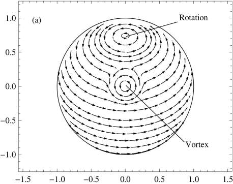
Figure 1: Streamlines of transverse circulations for three illustrating examples of tangential vortical motions over a spherical surface. The patterns of such vortical perturbation motions over spherical surfaces can be fairly arbitrary, while the magnitude of velocity perturbation increases inversely proportional to the radius of the collapsing stellar core due to the conservation of angular momentum. In the top panel, both a global spin of the collapsing stellar core with an embedded vortex are displayed. For the case of $w_{rot}\propto Y_{2,1}(\theta,\ \varphi)$, the circulation pattern over a spherical surface is shown in the middle panel; and that for the case of $w_{rot}\propto Y_{5,1}(\theta,\ \varphi)$ is displayed in the bottom panel.

Solving this radial vorticity perturbation equation of $w_{rot}$, a growing time dependence $e^{\tau/3}=|t|^{-1/3}$ for all spherical harmonic components of $w_{rot}$ can be readily derived. This temporal factor naturally shows an increase of the amplitude as $t\rightarrow-0^{-}$ for the radial component of vorticity perturbation by expression (30). A non-vanishing $w_{rot}$ leads to a perturbation solution for vortical motions with fairly arbitrary angular dependence in ($\theta,\ \phi$) superposed onto a dynamically collapsing stellar core without involving the radial component of velocity perturbation. These perturbation modes of $w_{rot}$ physically correspond to various vortical motions transverse to the radial direction $\mathbf{e_{r}}$. We emphasize that the only constraint on $w_{rot}$ is ODE (31), with no other spatial constraints (in terms of $x$) on $w_{rot}$. Therefore perturbation flow component patterns of $w_{rot}$ with various combinations of $\{l,\ \mathbf{m}\}$ are all allowed and can be superposed together with a set of proper coefficients to form fairly general or arbitrary circulation patterns. Meanwhile, it is quite clear that all $\{l,\ \mathbf{m}\}$ vortical modes share the same temporal growth factor $e^{\tau/3}$, and they may form rather random tangential vortical flow patterns according to the superposition principle. For the particular case of $l=1$, $\mathbf{m}=0$ as an example, we take $w_{rot}=x^{2}Y_{1,0}(\theta,\ \varphi)=x^{2}\cos\theta$, and then equation (28) gives an expression for the corresponding velocity perturbation as $\mathbf{v_{1}}=x\sin\theta\ \mathbf{e_{\varphi}}$; and this actually describes a global spin motion to perturb the radially collapsing stellar core. In the top panel of Figure 1, we show a tangential vortical flow pattern in which both a global spin of the stellar core and a relatively isolated vortex coexist. It is easy to understand the time dependence $e^{\tau/3}$ here by referring to expression (16). As can be seen, this type of vortical velocity perturbation is given by $\mathbf{u_{1}}=\dot{a}\mathbf{v_{1}}\propto e^{2\tau/3}\propto a^{-1}$. Noting also that $w_{rot}$ represents generally vortical perturbations (e.g. the above perturbation example of rotational motion) for which the angular momentum is conserved, it is then clear that the amplitude increase of this kind of vortical velocity perturbation results from the conservation of angular momentum and the rapid radial contraction of the stellar inner core size. For such growing vortical perturbation solutions, the perturbations in stellar pressure, mass density and gravitational potential ($f_{1},\ \beta_{1}\$and $\psi_{1}$) all remain zero (i.e. this is a type of incompressible flow perturbations).

The temporal growth factor $e^{\tau/3}$ here is faster than the temporal amplification factor $e^{\tau/6}$ for the oscillatory compressive normal modes [e.g. acoustic p$-$modes with $\gamma=\Gamma=4/3$ and $g(x)=1$]; this amplitude increase for all oscillatory p$-$modes corresponds to an adiabatic amplification of sound waves due to compression of the core collapse according to GW. In contrast, this faster $e^{\tau/3}$ growth factor reveals a non-oscillatory unstable amplitude increase of radial vorticity perturbation during the self-similar dynamic phase of a stellar core collapse. By our model scenario, the fast spin of a nascent PNS or a stellar mass black hole (identified as the collapsed stellar core remnant) is most likely triggered and gained during such an unstable growth of $l=1$, $\mathbf{m}=0$ vortical perturbations about the core collapse and concurrent nonlinear dynamic interactions.

There are alternative mechanisms proposed by others which might also contribute to the fast spin of a nascent PNS. Several years ago, Blondin & Mezzacappa (2007) suggested that the 3D growth of $l=1$ spiral modes (see their figures 1 and 2) of the SASI during the post-bounce delay phase may significantly spin up the core matter behind the stalled shock. We note more specifically that this type of SASI fluctuations is mainly of acoustic nature. In their 3D simulations, a nascent PNS has gained a considerable spin velocity with final periods of $\sim 70$ms for moderately rotating progenitors and $\sim 50$ms for non-rotating progenitors. In contrast, more recent numerical simulations (e.g. Iwakami et al. 2008; Rantsiou et al. 2011) seem to show that such $l=1$ spiral mode mechanism does not work so effectively and may only induce possible PNS spin periods of seconds. Blondin & Mezzacappa (2007) invoked several simplifications in their 3D simulations; they found that the nonlinear evolution of the SASI is dominated by low-order non-axisymmetric mode characterized by a spiral flow pattern beneath the accretion shock during the post-bounce delay phase (e.g. Blondin & Shaw 2007; Fernàndez 2010). Strictly speaking, they did not follow collapse itself, but started in a steady-state post-bounce configuration. Also, neutrino heating and cooling were neglected and the flow was assumed to be isentropic in Blondin & Mezzacappa (2007). In short, the issue of fast PNS spin remains open and should be explored further for vortical instabilities proposed here.

Conceptually for the dynamic core collapse of an extremely massive progenitor star (e.g. Lou & Wang 2006, 2007; Hu & Lou 2009; Lou & Wang 2011), a fast spinning central black hole may similarly form resulting from an unstable growth of such $l=1$ and $\mathbf{m}=0$ vortical perturbations. As an example of estimation, for a core collapse in which the stellar radius contracts by a factor of $\sim 10^{-3}$, an initial stellar spin angular velocity of $\sim 1-10$ cycles per day would lead to a spin angular velocity of $\sim 10-100$ cycle per second after the core collapse. Such effects might have already been observed in some numerical simulation works, e.g. Buras et al. (2006b), in which an initially specified stellar angular velocity is significantly amplified. This effect may considerably or even dominantly spin up a nascent PNS or a stellar mass black hole among other alternatives. Moreover, circulation speeds of any small or large vortices tangent to spherical surfaces within a dynamically collapsing stellar core will be amplified according to this $a^{-1}$ law; in other words, cyclones on spherical layer surfaces would spin faster and faster during such a dynamic core collapse.

It is conceivable that nonlinear interactions among such large-scale vortices within spherical layers and stellar core rotation would generate and sustain Rossby-type inertial waves (e.g. Haurwitz 1940; Lou 1987, 2000, 2001). Gravitational wave radiation carries angular momentum and may further excite stellar Rossby waves to set an upper limit on the spin rate of young neutron stars (e.g. Andersson et al. 1999; Dimmelmeier et al. 2008). If the stellar core collapse process is accompanied with seed magnetic fields, these fast increasing vortex perturbations nonlinear interactions might also induce magnetohydrodynamic (MHD) dynamo actions to enhance magnetic field strengths (e.g. Thompson & Duncan 1993; Hu & Lou 2009).

In the following general polytropic 3D perturbation analysis, we thus exclude the part involving $w_{rot}$, as we have already shown that it leads to unstable vortical perturbation solutions (i.e. radial component of vorticity perturbation) including the growth of rotational instability in a homologously collapsing stellar core. To separate the temporal component from the angular components of perturbation variables, we can consistently presume that $\psi_{1}$, $\beta_{1}$, $f_{1}$, $w_{r}$ and $w_{t}$ bear the two-dimensional (2D) angular dependence of spherical harmonics $Y_{l\mathbf{m}}(\theta,\ \varphi)$ and the temporal dependence $e^{n\tau}$ with $n$ being an additional parameter to be determined. Combining linearized equations (23), (24) and the two angular components of momentum perturbation equation (21) to eliminate the two dependent variables $\beta_{1}$ and $f_{1}$, it is straightforward to derive the following linear ODEs for 3D general polytropic compressible perturbations, namely

$$\frac{1}{x}\frac{\mbox{d}^{2}}{\mbox{d}x^{2}}(xn\psi_{1})-\frac{l(l+1)}{x^{2}}(n\psi_{1})-2f^{2}\bigg{[}\frac{f}{x^{2}}\frac{\mbox{d}}{\mbox{d}x}(x^{2}w_{r})$$

$$\qquad\qquad\qquad\qquad-\frac{l(l+1)f}{x}w_{t}+3f^{\prime}w_{r}\bigg{]}=0\ ,$$ (32)

$$\frac{4}{3}mxw_{t}-\gamma gf\bigg{[}\frac{1}{x^{2}}\frac{\mbox{d}}{\mbox{d}x}(x^{2}w_{r})-\frac{l(l+1)}{x}w_{t}\bigg{]}$$

$$\qquad\qquad\qquad\quad-(4gf^{\prime}+fg^{\prime})w_{r}-2(n\psi_{1})=0\ ,$$ (33)

$$\frac{4}{3}m\bigg{[}w_{r}-\frac{\mbox{d}}{\mbox{d}x}(xw_{t})\bigg{]}+[(4-3\gamma)gf^{\prime}+fg^{\prime}]$$

$$\qquad\quad\ \ \times\bigg{[}\frac{1}{x^{2}}\frac{\mbox{d}}{\mbox{d}x}(x^{2}w_{r})-\frac{l(l+1)}{x}w_{t}\bigg{]}=0\ .$$ (34)

In three linear perturbation ODEs (32)$-$(34) above, $f^{\prime}$ and $g^{\prime}$ are respectively the first derivatives of $f(x)$ and $g(x)$ with respect to $x$, and $m=3\lambda n(3n-1)/2$ is the eigenvalue parameter to be determined by proper physical requirements. This definition of the eigenvalue $m$ agrees with that of Cao & Lou (2009). In fact, equation (34) is simply the angular component of vorticity perturbation equation (25). Note that we can actually regard the product $n\psi_{1}$ as one dependent perturbation variable. Perturbation ODEs (32)$-$(34) are equivalent to vector equation (26).

For physically sensible perturbations, the relevant boundary conditions take the following form of

$$n\psi_{1}\propto x^{l}\ ,\qquad w_{r}=lw_{t}\propto x^{l-1}\qquad\ \mbox{for}\ x\rightarrow 0^{+}\ ,$$

$$n\psi_{1}\propto x^{-(l+1)}\qquad\qquad\qquad\qquad\qquad\mbox{for}\ x\rightarrow+\infty\ ,$$

$$\frac{mxw_{t}}{3}-gf^{\prime}w_{r}=\frac{n\psi_{1}}{2}\qquad\qquad\qquad\mbox{for}\ x=x_{b}\ ;$$ (35)

here $x_{b}$ stands for the value of $x$ at the moving boundary of the collapsing stellar core where the mass density $\rho_{0}$ vanishes. These boundary conditions are imposed to avoid singularity in perturbation solutions as $x\rightarrow 0^{+}$ and $x\rightarrow+\infty$. The condition at the contracting boundary $x_{b}$ requires a zero Lagrangian pressure perturbation there.

4 Model analysis and results for three-dimensional perturbations

4.1 A re-visit to GW model analysis and results

We first re-visit the special conditions adopted by GW, in which $\gamma=\Gamma=4/3$ and $g(x)=1$ for a constant specific entropy. It follows that our equation (34) reduces to

$$m\Big{[}w_{r}-\frac{\mbox{d}}{\mbox{d}x}(xw_{t})\Big{]}=0\ .$$ (36)

For this reason, GW choose to set $w_{r}=\mbox{d}(xw_{t})/\mbox{d}x$ with the eigenvalue parameter $m\neq 0$, leading to a kind of 3D potential flow velocity perturbation solutions representing only acoustic p$-$mode and f$-$mode oscillations in a homologously collapsing stellar core. This is because internal g$-$mode oscillations necessarily involve vorticity perturbations. Apparently, vorticity perturbations were completely excluded in the model analysis of GW.

In fact, there exist other perturbation solutions by setting $m=0$ in equation (36), corresponding to either $n=0$ or $n=1/3$ yet leaving the vorticity perturbation factor $[w_{r}-\mbox{d}(xw_{t})/\mbox{d}x]$ being fairly arbitrary in terms of $x$ [see also equation (25) with a vanishing RHS]. In the former case of $n=0$, all perturbations are neutrally stable, while the pressure, density and gravitational potential perturbations do not need to vanish in general. We now focus on the latter case of $n=1/3$, because in this case the perturbation is amplified during the self-similar core collapse process and is faster than the amplitude increase $e^{\tau/6}$ for the oscillatory acoustic p$-$modes due to adiabatic amplification of sound waves by compression in the core collapse. It can be demonstrated (see Appendix A for details) that to make equations (32) and (33) meet this demand for $n=1/3$, we must have

$$\frac{f}{x^{2}}\frac{\mbox{d}}{\mbox{d}x}(x^{2}w_{r})-\frac{l(l+1)f}{x}w_{t}+3f^{\prime}w_{r}=0\ ,$$ (37)

corresponding to mass conservation without mass density perturbation, i.e. the divergence of velocity perturbation vanishes. This can be easily confirmed by substituting equation (37) into perturbation ODEs (32) and (33). For these incompressible vorticity perturbation solutions, the pressure, density and gravitational potential are not disturbed. However, the time dependence of $e^{\tau/3}$ for $n=1/3$, which is faster than the contraction amplification factor $e^{\tau/6}$ for oscillatory acoustic p$-$modes in the dynamic background core collapse (see GW), indicates a relationship between these growing vorticity perturbation solutions and the angular momentum conservation (see the discussion on the temporal factor $e^{\tau/3}$ in Section 3). In fact, these perturbation solutions represent circulatory motions with non-vanishing vorticities, so it is natural that they develop according to the angular momentum conservation. In summary, we are left with ODE (37) where $[w_{r}-\mbox{d}(xw_{t})/\mbox{d}x]$ is an arbitrary function of $x$. By equation (25), this describes the growth of vortical convective motions, including in particular components of vorticity perturbation transverse to the radial direction.

We note that the mass density is not significantly disturbed in convective motions or vortex circulations; this feature also holds approximately for internal g-modes to be discussed further. In Buras et al. (2006b), they introduced arbitrary initial density fluctuations in the pre-bounce core collapse to examine effects of pre-bounce perturbations, and they found nothing obviously different except that the PNS convection starts slightly earlier. According to our analysis above, their perturbations are more likely of acoustic nature rather than convective motions and grow much slower, having relatively minor effects on the post-bounce phase.

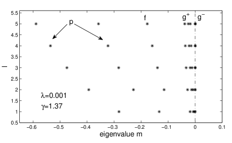
Figure 2: Eigenvalues of $m$ for the case of $\lambda=0.001$, $\gamma=1.37>\Gamma=4/3$ and $g(x)$ given by expression (39) as an example of illustration. The moving boundary of the stellar core is numerically determined at $x_{b}=6.9561$. In this case, both g${}^{+}-$modes (only three branches are shown) and g${}^{-}-$modes (only one branch is shown) exist. The eigenvalues of g${}^{-}-$modes (to the right of the vertical dash-dotted line) are quite close to zero. The eigenvalues of the first two orders of p$-$modes are on the left side. There are more branches of p$-$modes of higher orders with smaller eigenvalues of $m$ not shown in this figure. The unique f$-$mode branch with $l\geq 2$ separates p$-$modes and g$-$modes (n.b. the $l=1$ f$-$mode does not exist). If $\gamma$ value is higher, eigenvalues of g${}^{-}-$modes tend to vanish.

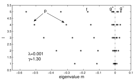
Figure 3: Eigenvalues of $m$ for the case of $\lambda=0.001$, $\gamma=1.30<\Gamma=4/3$ and $g(x)$ given by expression (39). The contracting boundary of the stellar core is numerically determined to be at $x_{b}=6.9561$. Compared to those shown in Figure 2, the eigenvalues of $m$ in this case are shifted towards the positive direction. The vertical dash-dotted line at $m=0$ separates nearby branches of g${}^{+}-$modes (left; only three branches are shown) from nearby branches of g${}^{-}-$modes (right; only three branches are shown). When the perturbation polytropic index $\gamma$ becomes sufficiently small, eigenvalues of g${}^{+}-$modes would completely disappear.

4.2 Computational Analysis and Explorations

In order to solve the perturbation eigenvalue problem posed here, we implement the procedure outlined below: first we use the fourth-order Runge-Kutta method (e.g. Press et al. 1986) to numerically integrate equation (15) for obtaining the self-similar background function $f(x)$ which is directly related to the dynamic background mass density $\rho_{0}(r,\ t)$ by equation (8). With this ready, we systematically discretize linear ODEs $(\ref{eq30})-(\ref{eq32})$ with a proper mesh to cast our 3D perturbation problem to a matrix eigenvalue problem with specified boundary conditions (35). The inverse iteration method (e.g. Wilkinson 1965) is then employed to search for the eigenvalues of $m$ and the corresponding eigenfunctions (see Appendix C for details of the numerical scheme).

We first solve the cases of globally constant specific entropy [i.e. $g(x)=1$] in space and time with $\gamma=\Gamma=4/3$, and the results of analysis agree quite well with those of Cao & Lou (2009) again confirming the errors of p$-$mode eigenvalues as computed by GW. We have also checked and confirmed the results of the sample solutions in Cao & Lou (2009) for several variable forms of $g(x)$ and $\gamma=\Gamma=4/3$ and in Cao & Lou (2010) for a constant $g(x)=1$ and several $\gamma\neq\Gamma=4/3$. With the assurance of a few necessary consistencies, we continue to apply our numerical codes to further explore the more general cases with a nontrivial variable $g(x)\neq 1$ and the polytropic exponent $\gamma\neq\Gamma=4/3$.

In stellar oscillations about static stars, there exist two types of g$-$modes (e.g. Cox 1976) which are distinguished by the sign of the square of the Brunt$-$V$\ddot{\rm a}$is$\ddot{\rm a}$l$\ddot{\rm a}$ buoyancy frequency ${\cal N}^{2}$ defined by

$${\cal N}^{2}\equiv{\cal G}\bigg{(}\frac{\partial\ln\rho_{0}}{\partial r}-\frac{1}{\gamma}\frac{\partial\ln p_{0}}{\partial r}\bigg{)}\ ,$$ (38)

where $\rho_{0}$ and $p_{0}$ are the background gas mass density and thermal pressure, respectively, ${\cal G}>0$ is the local gravitational acceleration and $\gamma$ is the polytropic exponent of 3D perturbations. For stellar oscillations, if ${\cal N}^{2}$ is positive everywhere, only g${}^{+}-$modes occur, whereas if ${\cal N}^{2}$ is negative everywhere, only g${}^{-}-$modes can be found.

For our self-similar core collapse case under consideration, definition (38) for ${\cal N}^{2}$ can be extended to allow $\rho_{0}$ and $p_{0}$ being also time-dependent for a dynamic background flow. Our numerical exploration demonstrates that if ${\cal N}^{2}$ is positive everywhere, the eigenvalues $m$ are always negative and only g${}^{+}-$modes occur, whereas if ${\cal N}^{2}$ is negative everywhere, the eigenvalues $m$ become always positive and only g${}^{-}-$modes can be found. As an example of illustration, we choose the dimensionless function $g(x)$ for the specific entropy evolution/distribution in the form of

$$g(x)=1+0.1x^{2}~{}\!\exp(-x^{2}/2)\ ,$$ (39)

and take $\lambda=0.001$ for the self-similar hydrodynamic background. In Figures 2 and 3, we show the eigenvalues $m$ for different spherical harmonic degree $l$ computed by setting $\gamma=1.37>4/3$ (Fig. 1) and $\gamma=1.30<4/3$ (Fig. 2), respectively. In our numerical exploration, it could be easily seen that the eigenvalues $m$ are shifted towards the positive direction when $\gamma$ decreases gradually. In Figures 2 and 3, both g${}^{+}-$modes and g${}^{-}-$modes exist. However, when the value of $\gamma$ is high enough (low enough), eigenvalues of g${}^{-}-$modes (g${}^{+}-$modes) will disappear by examining the trends of extensive numerical results. This can also be seen from definition (38) of the Brunt$-$V$\ddot{\rm a}$is$\ddot{\rm a}$l$\ddot{\rm a}$ buoyancy frequency squared ${\cal N}^{2}$. Note that the eigenvalues $m=3\lambda n(3n-1)/2$ of g$-$modes are all fairly close to $0$, corresponding to approximately temporal growth factors around $e^{\tau/3}=|t|^{-1/3}$ for the amplitude of oscillations when $n\sim 1/3$.

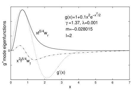
Figure 4: The eigenfunctions for the lowest order g${}^{+}-$mode with $\lambda=0.001$, $\gamma=1.37$, $l=2$ and $g(x)$ given by expression (39) (see Fig. 2 for sample eigenvalues). The moving boundary of the collapsing stellar core is at $x_{b}=6.9561$. The oscillation is primarily confined within the central region of the collapsing stellar core.

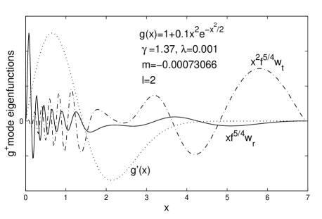
Figure 5: A higher order $g^{+}-$mode with $\lambda=0.001$, $\gamma=1.37$, $l=2$ and $g(x)$ given by expression (39). The moving boundary of the collapsing stellar core is at $x_{b}=6.9561$. The oscillation overcomes the barrier where $g^{\prime}(x)<0$ and approaches the outer part of the stellar core. This appears to be a kind of wave tunneling effect.

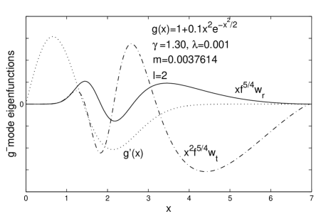
Figure 6: An example of g${}^{-}-$mode with $\lambda=0.001$, $\gamma=1.30$, $l=2$ and a background profile $g(x)$ given by expression (39). The moving boundary of the stellar core is at $x_{b}=6.9561$. The oscillations are confined inside the region where $g^{\prime}(x)<0$.

In Figure 4, we show the lowest order of g${}^{+}-$modes for the case $\gamma=1.37$. The solid curve stands for the scaled eigenfunction $xf^{5/4}w_{r}$ (related to the radial velocity perturbation), and the dash-dotted curve represents the scaled eigenfunction $x^{2}f^{5/4}w_{t}$ (related to the transverse velocity perturbation). We also show the curve of the function $g^{\prime}(x)$ by the dotted curve [see expression (39) for the form of $g(x)$]. It can be seen that the oscillatory wave pattern of the eigenfunctions are mainly trapped within the collapsing stellar core. However, the patterns are no longer confined inside the region where $g^{\prime}(x)>0$, which is different from the parallel results in the case of $\gamma=4/3$ (see Cao & Lou 2009). In Figure 5, we further exhibit a higher order g${}^{+}-$mode. It is clear that the oscillatory wave patterns are also mostly confined inside the collapsing stellar core, but the waves seem to overcome the barrier region (e.g. Lou 1995a,b, 1996) where $g^{\prime}(x)$ is negative, and are amplified when approaching the outer boundary of the stellar core. In the case of $\gamma\leq 4/3$, however, this wave tunneling does not happen. This effect seems to be due to the increase of $\gamma$ value. Another feature of these deeply trapped g${}^{+}-$modes is that the radial oscillation dominates, while the horizontal oscillation decreases inside the collapsing stellar core.

Figure 6 shows one of the g${}^{-}-$modes in the case of $\gamma=1.30$, as an example of the cases $\gamma<\Gamma=4/3$. The oscillatory behaviours of g${}^{-}-$modes are mostly confined within a region of $g^{\prime}(x)<0$.

In Figure 7, we show a lowest order unstable g${}^{+}-$mode for $\lambda=0.006$, $\gamma=4/3$, $l=1$ and $g(x)$ prescribed as

$$g(x)=1+0.001x^{2}\exp(-x^{2}/2)\ .$$ (40)

This g${}^{+}-$mode has an eigenvalue $m=-0.00014539$. Recalling the eigenvalue definition of $m=3\lambda n(3n-1)/2$, we find either $n=0.3163$ or $n=0.0170$. The former is larger than $1/6$ and corresponds to an unstable temporal growth. As will be discussed in Section 4.3 presently, the $l=1$ mode can lead to a displacement of the very centre of the stellar core. Such unstable core displacement along with nonlinear dynamic evolution may give rise to systematic movement of the collapsed core during the emergence of a reverse shock. Note that this mode is mostly confined inside the collapsing stellar core, so the displacement of the centre of the core will be more pronounced than that of the outer part. We therefore propose that the rapid increase of this unstable central core displacement may be ultimately responsible for the initial kick process of nascent PNSs or stellar mass black holes produced in SN remnants (see Section 4.3 and estimates in Cao & Lou 2009).

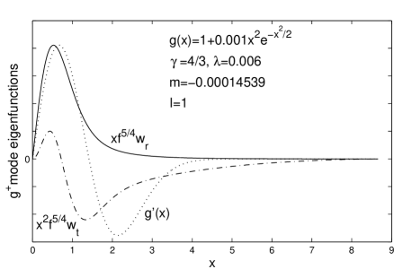
Figure 7: An unstable lowest order g${}^{+}-$mode with $\lambda=0.006$, $\gamma=4/3$, $l=1$ and $g(x)$ given by expression (40). The contracting boundary of the collapsing stellar core is at $x_{b}=8.6598$. The corresponding $n$ value is either $0.3163$ or $0.0170$. This lowest order unstable g${}^{+}-$mode with $l=1$ may describe a kick of nascent collapsed compact object (e.g. PNS or stellar mass black hole left behind in a SN remnant).

Other assigned evolutions or distributions of the specific entropy function $g(x)$ have also been explored, including the following three different forms

$$g(x)=1+\frac{0.01x^{2}}{0.01x^{2}+1}\ ,$$ (41)

$$g(x)=1-\frac{0.01x^{2}}{2(0.01x^{2}+1)}\ ,$$ (42)

$$g(x)=1+0.1x^{2}(x-2)(x-4)\exp(-x^{2}/9)\ .$$ (43)

The results of numerical solutions for 3D general polytropic perturbations are consistent with the earlier conclusion that g${}^{+}-$modes are mainly confined within the regime with $g^{\prime}(x)>0$, and that g${}^{-}-$modes dominate in the region of $g^{\prime}(x)<0$. The specific oscillatory wave pattern may be influenced by the choice of the polytropic index $\gamma$ for 3D perturbations. Regarding the last expression of $g(x)$ as defined by equation (43) or other similar expressions for which the first derivative $g^{\prime}(x)$ crosses the value $0$ more than once, the region $g^{\prime}(x)>0$ [$g^{\prime}(x)<0$] are divided into several intervals in the $x$ domain, the corresponding g${}^{+}-$modes (g${}^{-}-$modes) appear to have the trend to concentrate inside the interval nearest to the stellar interior core. This indicates that g$-$modes are mainly trapped deeply inside the central region of a collapsing stellar core.

4.3 Physical Nature of Perturbation Instabilities

We have shown in Figures 2 and 3 that the eigenvalues of $m$ for g$-$modes can be quite close to $0$ especially for higher radial orders (i.e. the anti-Sturmian property). As the specific entropy profile $g(x)$ tends to constant $1$ and $\gamma$ approaches $\Gamma=4/3$ simultaneously, the absolute value of buoyancy frequency squared $|{\cal N}^{2}|$ becomes smaller and smaller, squeezing all eigenvalues $m$ of g$-$modes to converge towards zero.

As shown in Section 4.1, we reveal a type of unstable perturbation solutions with eigenvalue $m=0$ ($n=1/3$) in that very limit of $g(x)=1$ and $\gamma=4/3$. Growing with time $t$, these are purely vortical perturbations with $\mathbf{e_{\theta}}$ and $\mathbf{e_{\varphi}}$ components [see eq. (25)]; meanwhile mass conservation (37) should be satisfied in the absence of mass density perturbation (see Appendix A for details). In other words, the three components of vorticity perturbation $(\nabla\times{\mathbf{v}_{1}})$ all behave in the same temporal manner of unstable growth [see eqns (30) and (31)] with arbitrary dependence of $(x,\ \theta,\ \varphi)$. Physically, they describe unstable vortical convections and circulations in a dynamically collapsing stellar core. It would be more convenient and precise to regard them as separate vorticity modes of instability.

Complementarily, we may equally view such vortical perturbations as infinitely degenerate g$-$modes with eigenvalue $m=0$ ($n=1/3$). In reference to equation (34), we can imagine the dimensionless specific entropy $g(x)$ to approach constant $1$ and the perturbation polytropic exponent $\gamma$ to approach the background $\Gamma=4/3$; given the fact that perturbation variable $w_{r}-\mbox{d}(xw_{t})/\mbox{d}x$ (related to $\mathbf{e_{\theta}}$ and $\mathbf{e_{\varphi}}$ components of vorticity perturbation) does not vanish for g$-$modes, it is then clear that all eigenvalues of $m$ concentrate towards $0$. In that limiting regime, all g$-$modes would become completely degenerate. This also explains why vortical perturbation solutions obtained in Section 4.1 can have arbitrary vortical configurations as long as that the mass conservation (37) is satisfied without inducing mass density perturbation. Therefore we may state that amplitude growths of g$-$modes in general are primarily governed by the angular momentum conservation (see Appendix D). This implies that perturbation amplitudes of g$-$modes are roughly inversely proportional to the radius of the collapsing stellar core. This conclusion should remain valid for a stellar core collapse with background polytropic exponent $\Gamma\neq 4/3$, for there should also exist amplification of perturbations resulting from the angular momentum conservation. In general, growth rates of g$-$modes are also modified by the variable specific entropy evolution/distribution $g(x)$ as well as the corresponding $\lambda$ value and the difference between the perturbation polytropic exponent $\gamma$ and the background polytropic exponent $\Gamma=4/3$. Sufficiently high-order g${}^{+}-$modes and all g${}^{-}-$modes are unstable, that is, they grow faster than the temporal factor $|t|^{-1/6}$ for stable acoustic p$-$modes and f$-$modes associated with a self-similar stellar core collapse (GW; Lou & Cao 2008).

Such g$-$mode instabilities mainly governed by the angular momentum conservation might have a significant influence on the pre-SN core collapse stage and may affect the appearance of the PNS born during the stellar core collapse and the emergence of rebound shock as well as an SN explosion. The effects of these unstable g$-$modes and vortical circulation modes during a stellar core collapse might have been omitted in previous multi-dimensional simulation works (e.g. Buras et al. 2006a; Dessart et al. 2006; Nordhaus et al. 2010b), because of their characteristic feature of weak or no density fluctuations. Many numerical simulations show that the neutrino luminosity is not high enough to trigger an SN explosion. It is considered physically plausible that the neutrino driven convection plays a key role in an SN explosion. Our fast growing hydrodynamic convective g-modes and/or vorticity modes during a stellar core collapse, if properly included, might supply additional strengths for the PNS neutrino convection and circulation. These unstable perturbations will naturally destroy the spherical symmetry of the collapsing stellar core and give rise to subsequent aspherical nonlinear dynamic interactions. The resulting asymmetric disturbances might actually be connected to and affect the initiation and evolution of SASI, although SASI is primarily of acoustic nature and operates between PNS and the stalled bounce shock. In fact, g$-$mode oscillations of a PNS may also accompany SASI during the bounce phase (e.g. Burrows et al. 2006). Our internal g$-$mode, vortical and convective instabilities exist during the core collapse irrespective of details of the specific entropy distribution/evolution.

Among all these unstable g$-$modes, those with $l=1$ allow a non-vanishing bulk flow velocity at the very centre of the progenitor stellar core. These unstable g$-$modes may contribute directly or indirectly to the observed high peculiar speed of a new-born PNS (remnant of a stellar core collapse), which may reach values of several hundred to more than one thousand kilometers per second. As an estimation, we assume the initial gas bulk flow velocity of the stellar core relative to the center of mass of the entire star to be $\sim 200\ {\rm m\ s}^{-1}$, and the radius of the collapsing PNS contracts by a factor of $\sim 10^{-3}$, then the stellar core will gain a velocity around $\sim 200\ {\rm km\ s}^{-1}$ as a result of the rapid growth of $l=1$ g$-$mode perturbations, provided that the linear approximation still remains valid. The smaller this contraction factor, the higher the PNS kick speed; the phase of PNS $l=1$ g$-$mode oscillation, the proper timing of stellar core collapse and the overall flow environment together should be also important to determine the net kick efficiency. The initiation of such a collapsing PNS kick may actually occur prior to the emergence of a bounce shock. Recent numerical simulation studies suggest that the neutron star kick may be produced by the gravitational pull of the post-bounce anisotropic slow-moving ejecta (see figure 7 of Scheck et al. 2006) which may result from the neutrino-driven convection (e.g. Scheck et al. 2004; Nordhaus et al. 2010a). For example, based on extensive 2D model simulations with approximate neutrino transport and boundary conditions that parameterize the effects of the contracting NS and strong enough neutrino heating for neutrino-driven SN explosions, Scheck et al. (2006) compared their results with those of Burrows et al. (2006). Started 20 ms after the core bounce, the simulation results of Scheck et al. (2006) can lead to a dominance of dipole ($l=1$) and quadruple ($l=2$) modes in the explosion ejecta, provided that the onset of the SN explosion is sufficiently slower than the growth time scale of the low-mode instability; they show that global anisotropies and large NS kicks can be obtained naturally in the framework of the neutrino-driven SN explosion mechanism due to the symmetry breaking by non-radial hydrodynamic instabilities, without resorting to rapid rotation, large pre-collapse perturbations in the iron core, strong magnetic fields, anisotropic neutrino emission associated with exotic neutrino properties, or jets etc. As a complement to the work of Scheck et al. (2006), Nordhaus et al. (2010a) performed a 2D axisymmetric radiation-hydrodynamic simulation of the collapse of a non-rotating 15$M_{\odot}$ progenitor core and can naturally capture the PNS formation and subsequent off-center acceleration during a delayed, neutrino-driven, anisotropic SN explosion (their SN explosion is artificially induced by including additional neutrino luminosity to the calculation); at the end of their simulation, the PNS has achieved a velocity of $\sim 150\hbox{ km s}^{-1}$ and is still accelerating at $\sim 350\hbox{ km s}^{-2}$. In the simulation of Burrows et al. (2006), the acoustic energy input from PNS g-mode oscillations was crucial for the explosion of an 11$M_{\odot}$ progenitor. Nonspherical accretion was found to give rise to core g-mode oscillations at late times ($\;\lower 4.0pt\hbox{${\buildrel\displaystyle>\over{\sim}}$}\;300-500$ms) after core bounce, providing a significant amount of acoustic power for SN shock. Actually, g-mode oscillations are also present in the outer layer of a NS according to Scheck et al. (2006), but the amplitudes are modest and do not lead to the strong effects of Burrows et al. (2006). It is possible that Scheck et al. (2006) simulations might underestimate g-mode effects which would require the inclusion of the entire neutron star without excising the central core and thus the dynamic coupling among accretion, core motion, and deep g-mode generation in a self-consistent manner. According to our estimates above, the core collapse hydrodynamic convective instabilities may also have a significant impact on the development of the anisotropic ejecta and the asymmetric bounce shock, and may also contribute directly to the PNS kick, providing a pre-existing background velocity during the formation of a nascent PNS. It would be desirable that these sources of g$-$mode instabilities during core collapse be further explored by 3D numerical simulations. In addition, those unstable g$-$modes with $l=2$ might induce a collapsing stellar core to break up into two pieces, forming binary PNSs or other combinations around the centre of the pre-SN progenitor, while g$-$modes with higher $l$ and under favorable conditions may violently destroy the stellar core, shredding it into many smaller pieces and thus leading to the destruction of a PNS. The possibility of such a situation might be low, as several multi-dimensional numerical simulations show that low$-l$ modes appear most likely dominant.

Based on our model analysis, the vorticity modes of instability appear unavoidable during a stellar core collapse; this would happen irrespective of the specific entropy evolution/distribution $g(x)$ including the conventional polytropic case of $g(x)=1$. Depending on sources of seed fluctuations, rapid core spin, circulations of various scales, and vortical convections would go along with the stellar core collapse in a generic manner. Physically, such 3D vortical motions can naturally lead to core convective turbulence and thus MHD dynamo actions for producing intense magnetic fields in PNSs and in stellar mass black holes. Conceptually, we may specifically separate the stellar core rotation from the rest of radial vorticity perturbation [see eq. (31)] and envision the scenario of nonlinear Rossby waves (e.g. Haurwitz 1940; Lou 1987, 2001).

5 Summary and Conclusions

3D general polytropic perturbations in a $\Gamma=4/3$ self-similar collapsing stellar core have been examined. We combine two recent generalized formulations adopted by Cao & Lou (2009, 2010) together to explore even more general cases of 3D perturbations. The specific entropy evolution/distribution profile $g(x)$ is allowed to vary from the stellar centre to its outer contracting boundary. The special subcase of uniform $g(x)=1$ corresponds to a conventional polytropic gas sphere (GW; Lou & Cao 2008). The polytropic exponent $\gamma$ of 3D perturbations is generally allowed to be different from the background polytropic exponent $\Gamma=4/3$. Not surprisingly, these general conditions give a non-zero Brunt-V$\ddot{\rm a}$is$\ddot{\rm a}$l$\ddot{\rm a}$ buoyancy frequency squared ${\cal N}^{2}$ as defined by equation (38), and allow for two groups of g$-$mode perturbations to occur, viz. g${}^{+}-$modes and g${}^{-}-$modes under proper situations. Meanwhile, acoustic p$-$modes and f$-$modes can also be clearly identified from the results of numerical calculations; again, they remain stable.

We first revealed a class of unstable radial vorticity perturbation solutions that are incompressible and can be separated out independently from the rest of compressible perturbation variables under fairly general situations, i.e. irrespective of the specific entropy evolution/distribution profile $g(x)$. Such unstable vortical perturbations include the spin of the collapsed stellar core and all kinds of sufficiently slow vortex motions tangent to spherical layers in the stellar core. Their velocity amplitudes are inversely proportional to the radius of the collapsed stellar core, as a result of the angular momentum conservation. This appears to be a natural mechanism for producing fast spins of PNSs or stellar mass black holes in the eventual nonlinear evolution. Conceptually, one may further separate the core spin and other radial vorticity perturbations; their mutual nonlinear interactions and evolution may be perceived. We therefore suggest that Rossby waves may occur and be amplified in nonlinear dynamic processes. Such Rossby waves may be also connected with the spin down process of a nascent neutron star. If the collapsing stellar core is magnetized, significant MHD dynamo actions may also take place to amplify magnetic fields during the core collapse process involving considerable turbulent convections and circulations.

By the inverse iteration method (e.g. Wilkinson 1965), we then solve the remaining general polytropic compressible perturbation equations (32)$-$(34) numerically with specified boundary conditions (35), and examine the eigenvalues and eigenfunctions of perturbations, including acoustic p$-$modes, surface f$-$modes and internal g$-$modes, which can be further divided into two subclasses: internal g${}^{+}-$modes and internal g${}^{-}-$modes. Sufficiently high radial order g${}^{+}-$modes and all g${}^{-}-$modes show instabilities during the dynamic core collapse process, leading to convective motions of circulation within the collapsing stellar core. In contrast, acoustic p$-$modes, f$-$modes and sufficiently low order g${}^{+}-$modes remain stable. For a certain specific entropy evolution/distribution, there may exist g$-$modes that are drastically oscillatory deeply trapped in the collapsing stellar core.

The mechanism of unstable growths of g$-$modes is identified. We realize that the fast temporal increase in amplitudes of g$-$modes are mainly governed by the angular momentum conservation. It is easy to understand this intuitively, for g$-$mode perturbations are mainly convective motions inside the dynamically collapsing stellar core, in which the gas runs in circulations. During the core collapse, the velocity of the gas flow will increase accordingly (see Appendix D for more details). In a more realistic model for stellar core collapse, both $\kappa$ and $\Gamma$ may vary in time. However, during a long period before the end of the collapse of stellar core, numerical simulations (e.g. Burrows & Lattimer 1986; Van Riper & Lattimer 1981; Bethe 1990) show that the variations of $\kappa$ and $\Gamma$ are slow and not obvious, and our conclusions may still be valid approximately. The amplitude of g$-$mode perturbations are more or less inversely proportional to the radius of collapsing stellar core. When the specific entropy distributes uniformly and the perturbation polytropic exponent $\gamma=\Gamma=4/3$, this temporal increasing factor of perturbation amplitude becomes exact, and all the g$-$modes become completely degenerate in this regard. Alternatively, we can regard these unstable modes as 3D vorticity perturbations constrained by the mass conservation. They may bear physical consequences for the central compact object, be it PNSs or stellar mass black holes.

Given the idealizations and approximations of our model, these unstable g$-$modes may offer certain valuable clues for SN model simulations. They affect the geometry of the rebound shock wave emerged after the core bounce because of asymmetries and enhance the neutrino driven PNS convection. Most simulation works do not explicitly include these convective g-mode perturbations (e.g. Dessart et al. 2006; Nordhaus et al. 2010b). Buras et al. (2006b) added in their simulation an arbitrary density perturbation before the core collapse, and do not observe significant difference. The density perturbations, however, are likely more acoustic and grow slowly, because the convective g-modes involve weak density fluctuations. Among the various g-modes, the $l=1$ g$-$modes with central movement may possibly be responsible for the origin of the high kick speed that a new-born neutron star acquires, or serve as the source of producing anisotropic stellar ejecta which may possibly gravitationally accelerate a nascent PNS (Scheck et al. 2006; Nordhaus et al. 2010a). Nonlinear evolution of those unstable g$-$modes with $l$ higher than $1$ may possibly break a collapsing core into two or multiple pieces, forming a binary system of neutron stars or more fragments as to even ultimately prevent the formation of a neutron star.

Instabilities of radial component vorticity perturbation can lead to rapid rotations of central compact objects, Rossby waves, and circulations over spherical surfaces inside a core. Instabilities of 3D vorticity perturbation when $g(x)=1$ and $\gamma=\Gamma=4/3$ can give rise to convective turbulence in the core and MHD dynamo actions to sustain violent magnetic activities.

Appendix A Equation (35) is necessary given $\gamma=4/3$, $g(x)=1$ and $m=0$

In the special case of $\gamma=4/3$, $g(x)=1$ and $m=0$ for a conventional polytropic gas, equation (34) is automatically satisfied. In the first subcase of $n=0$, equation (37) comes out automatically from equation (32). When we focus on the other subcase of $n=1/3$ satisfying the same requirement $m=0$, we derive from equation (33) the following relation

$$\psi_{1}=-2\bigg{[}\frac{f}{x^{2}}\frac{\mbox{d}}{\mbox{d}x}(x^{2}w_{r})-\frac{l(l+1)f}{x}w_{t}+3f^{\prime}w_{r}\bigg{]}\ ;$$ (44)

meanwhile equation (32) yields

$$\frac{\mbox{d}^{2}(x\psi_{1})}{\mbox{d}x^{2}}=\bigg{[}\frac{l(l+1)}{x^{2}}-3f^{2}\bigg{]}(x\psi_{1})\ .$$ (45)

In the interval $(x_{b},\ +\infty)$, we define $f(x)=0$. To avoid singularity, we naturally require $x\psi_{1}$ to remain finite at $x=0$ and $x\rightarrow+\infty$. Equation (32) should be regarded as a Sturm-Liouville problem within the interval $[0,\ +\infty)$ for determining the eigenvalues $l(l+1)$. The eigenvalues $l$ are determined by the specific profile of the dynamic background density function $f(x)$ and in general cannot be exactly equal to an integer. This means that in general we could only have the trivial solution $x\psi_{1}=0$ for integral values of $l$. Another argument proving the necessity of $x\psi_{1}=0$ can be made in the following for those cases $l\geq 2$. Since $x\psi_{1}$ should remain finite at $x=0$ to avoid singularity of a proper perturbation solution, $x\psi_{1}\propto x^{l+1}$ should hold as $x\rightarrow 0^{+}$. We also need to require $x\psi_{1}\propto x^{-l}$ when $x\rightarrow+\infty$ so that $\psi_{1}$ approaches zero at infinity. This means that the algebraic sign of $\mbox{d}(x\psi_{1})/\mbox{d}x$ should necessarily reverse when $x$ varies from $0^{+}$ to $+\infty$. Suppose that $x\psi_{1}$ is positive when $x\rightarrow 0^{+}$, then its first derivative is also positive. However, from the numerical results of $f(x)$ it is found that for $l\geq 2$, inequality $l(l+1)/x^{2}-3f^{2}>0$ holds in the entire interval $(0,+\infty)$, which indicates that $\mbox{d}^{2}(x\psi_{1})/\mbox{d}x^{2}$ remains positive as long as $x\psi_{1}$ is positive. There seems no chance for the sign of $\mbox{d}(x\psi_{1})/\mbox{d}x$ to reverse. Then $x\psi_{1}$ must vanish. In conclusion, we show that $x\psi_{1}=0$, and according to equation (A1), the necessity of equation (37) is warranted.

Appendix B Orthogonal set of eigenfunctions with distinct eigenvalues $m$

Perturbation eigenfunctions with different eigenvalues of $m=3\lambda n(3n-1)/2$ can be proven to be mutually orthogonal to each other. In the proof below, we use superscripts ⁽¹⁾ and ⁽²⁾ to distinguish different eigenfunctions and eigenvalues. From perturbation equations (22) and (23), we readily find

$$\nabla^{2}\frac{\partial\psi_{1}}{\partial\tau}=2\nabla\cdot(f^{3}\mathbf{v_{1}})\ ;$$ (46)

a substitution of equations (23) and (24) into equation (21) then yields

$$\frac{4}{3}mf^{3}\mathbf{v_{1}}=\nabla\Big{[}\gamma gf^{4}(\nabla\cdot\mathbf{v_{1}})+\mathbf{v_{1}}\cdot\nabla(gf^{4})\Big{]}$$

$$\qquad\ \quad-\Big{(}\nabla\cdot\mathbf{v_{1}}+\mathbf{v_{1}}\cdot\frac{3\nabla f}{f}\Big{)}\nabla(gf^{4})+2f^{3}\nabla\frac{\partial\psi_{1}}{\partial\tau}\ .$$ (47)

We now evaluate the spatial integral below with the help of equations (46) and (47), namely

$$\quad\frac{4}{3}m^{(1)}\int f^{3}\mathbf{v_{1}}^{(1)}\cdot\mathbf{v_{1}}^{(2)}\mbox{d}V$$

$$=-\int\Big{[}\gamma gf^{4}\nabla\cdot\mathbf{v_{1}}^{(1)}+\mathbf{v_{1}}^{(1)}\cdot\nabla(gf^{4})\Big{]}\nabla\cdot\mathbf{v_{1}}^{(2)}\mbox{d}V$$

$$\quad-\int\bigg{[}\nabla\cdot\mathbf{v_{1}}^{(1)}+\mathbf{v_{1}}^{(1)}\cdot\frac{3\nabla f}{f}\bigg{]}\nabla(gf^{4})\cdot\mathbf{v_{1}}^{(2)}\mbox{d}V$$

$$\quad-\int 2\frac{\partial\psi_{1}^{(1)}}{\partial\tau}\nabla\cdot\big{[}f^{3}\mathbf{v_{1}}^{(2)}\big{]}\mbox{d}V$$

$$=-\int\bigg{\{}\gamma gf^{4}\big{[}\nabla\cdot\mathbf{v_{1}}^{(1)}\big{]}(\nabla\cdot\mathbf{v_{1}}^{(2)})$$

$$\qquad+\big{[}\mathbf{v_{1}}^{(1)}\cdot\nabla(gf^{4})\big{]}(\nabla\cdot\mathbf{v_{1}}^{(2)})$$

$$\qquad+\big{[}\mathbf{v_{1}}^{(2)}\cdot\nabla(gf^{4})\big{]}(\nabla\cdot\mathbf{v_{1}}^{(1)})$$

$$\qquad+\big{[}\mathbf{e_{r}}\cdot\mathbf{v_{1}}^{(1)}\big{]}\big{[}\mathbf{e_{r}}\cdot\mathbf{v_{1}}^{(2)}\big{]}\frac{3\nabla f\cdot\nabla(gf^{4})}{f}$$

$$\qquad-\Big{(}\nabla\frac{\partial\psi_{1}^{(1)}}{\partial\tau}\Big{)}\cdot\Big{(}\nabla\frac{\partial\psi_{1}^{(2)}}{\partial\tau}\Big{)}\bigg{\}}\mbox{d}V\ ,$$ (48)

where $dV$ is the volume element for the spatial integration. Noting that the RHS of equation (48) is symmetric with respect to two superscripts ⁽¹⁾ and ⁽²⁾, we have

$$\big{[}m^{(1)}-m^{(2)}\big{]}\int f^{3}\mathbf{v_{1}}^{(1)}\cdot\mathbf{v_{1}}^{(2)}\mbox{d}V=0\ ,$$ (49)

and the orthogonality of eigenfunctions with different eigenvalues of $m$ is therefore proven.

Appendix C Inverse Iteration Scheme for Solving Linear ODEs (30)$-$(32)

We give here a procedure description of the inverse iteration scheme (e.g. Wilkinson 1965) as adapted to our numerical computations of 3D general polytropic perturbations in a self-similar dynamic stellar core collapse of spherical symmetry and $\Gamma=4/3$.

First, we specify a chosen form of the specific entropy function $g(x)$ and employ the fourth-order Runge$-$Kutta scheme (e.g. Press et al. 1996) to integrate background ODE (15) for $f(x)$ from $x=0^{+}$ and thus obtain the dynamic background function $f(x)$ with the initial or boundary conditions $f(0)=1$ and $f^{\prime}(0)=0$; this $f(x)$ is closely related to the background mass density profile. For $\Gamma=4/3$, the contracting boundary of the stellar core $x_{b}$ is determined by the realizable requirement $f(x_{b})=0$ in a parameter range of $0<\lambda\leq\lambda_{c}$ for a proper $\lambda$ value. Our goal is to reliably solve linear ODEs (32)$-$(34) for 3D general polytropic compressible perturbations within the interval $[0,\ x_{b}]$ by determining the eigenvalues of $m=3\lambda n(3n-1)/2$ and the corresponding perturbation eigenfunctions for given $g(x)$, $f(x)$, $\lambda$, $x_{b}$, $l$ and $\gamma\neq\Gamma=4/3$ in general.

In order to implement the inverse iteration scheme, we need to discretize linear ODEs (32)$-$(34) with a proper mesh in the interval $(0,\ x_{b})$. More specifically, we first divide the entire interval evenly into $N$ small intervals and define the interval size $\Delta x\equiv h=x_{b}/N$; we can then construct a vector $\mathbf{w}$ of length $2(N-1)$ for $w_{r}$ and $w_{t}$ arranged together contiguously in order, namely

$$\mathbf{w}=\Big{[}w_{r}(h),w_{r}(2h),\cdots w_{r}((N-1)h),$$

$$\qquad\qquad w_{t}(h),w_{t}(2h),\cdots w_{t}((N-1)h)\Big{]}^{T}\ .$$ (50)

We also need to cast every differential operator into a matrix form. The matrix for a function serving as coefficients in the ODEs, say $y(x)$, would then take the form of

$$Y=Diag\Big{[}y(h),y(2h),\cdots y((N-1)h)\Big{]}\ ,$$ (51)

which is a matrix of dimension $(N-1)$. By notation ‘$Diag$’, we refer to a diagonal matrix. The matrices $D$ and $D^{2}$ for the differential operators $\mbox{d}/\mbox{d}x$ and $\mbox{d}^{2}/\mbox{d}x^{2}$ are respectively

$$D=\frac{1}{h}\left(\begin{array}[]{ccccc}1&&&&\\ -1&1&&&\\ &-1&1&&\\ &&\cdot&\cdot&\cdot\\ &&&-1&1\\ \end{array}\right)\$$ (52)

and

$$D^{2}=\frac{1}{h^{2}}\left(\begin{array}[]{ccccc}-2&1&&&\\ 1&-2&1&&\\ &1&-2&1&\\ &&\cdot&\cdot&\cdot\\ &&&1&-2\\ \end{array}\right)\ ,$$ (53)

both are of dimension $(N-1)$. For different boundary conditions, these matrices above may need modifications accordingly. Note that ODE (33) can be substituted into ODE (32) to eliminate the dependent variable $n\psi_{1}$. With these procedures, we could finally achieve the discretization scheme of linear ODEs (32)$-$(34). The resulting finite difference scheme can be simply cast into the following form of

$$\left(\begin{array}[]{cc}A_{1}&A_{2}\\ A_{3}&A_{4}\end{array}\right)\mathbf{w}=A\mathbf{w}=m\mathbf{w}\ ,$$ (54)

in which $A_{i}\ (i=1,2,3,4)$ are four matrices all of dimension $(N-1)$ that do not involve the eigenvalue parameter $m$; here, eigenvalue parameter $m$ appears only on the RHS and is to be determined for discrete eigenvalues.

We can then apply the inverse iteration method to solve this eigenvalue problem. We begin to specify an arbitrary vector $\mathbf{w}_{0}$ and guess an approximate eigenvalue $m_{0}$, and then rewrite the matrix equation (54) as

$$(A-m_{0})\mathbf{w}=(m-m_{0})\mathbf{w}\ .$$ (55)

Suppose that all the eigenvalues and eigenfunctions of matrix equation (54) are respectively $m_{i}$ and $\mathbf{w}_{i}\ (i=1,2,\cdots)$, among which the value of $m_{j}$ is closest to the initially chosen value $m_{0}$. Then, $\mathbf{w}_{0}$ can be expanded as $\mathbf{w}_{0}=\sum_{i}a_{i}\mathbf{w}_{i}$, where $a_{i}$ stands for a set of coefficients, and it is thus easy to demonstrate

$$(A-m_{0})^{-n}\mathbf{w_{0}}\rightarrow a_{j}(m_{j}-m_{0})^{-n}\mathbf{w_{j}}\quad\mbox{as}\quad n\rightarrow\infty\ .$$ (56)

Therefore, by iterating an enough number of times, we can select the eigenfunction $\mathbf{w}_{j}$ and determine the corresponding eigenvalue $m_{j}=(m_{j}-m_{0})+m_{0}$. Changing the value of $m_{0}$, we would be able to select other eigenfunctions and eigenvalues of the perturbation problem.

Appendix D Magnitude growth of g-modes during a core collapse by angular momentum conservation

The angular momentum in a certain spatial volume $V$ of first-order precision can be cast in the integral form of

$$\mathbf{J}_{V}=\int_{V}\rho(\mathbf{r}\times\mathbf{u})d^{3}\mathbf{r}=\Big{(}\frac{\kappa_{c}}{\pi G}\Big{)}^{3/2}\dot{a}a\int_{V}f^{3}(\mathbf{x}\times\mathbf{v_{1}})d^{3}\mathbf{x}$$

$$\qquad\qquad={\cal A}e^{\tau/3}\int_{V}f^{3}(\mathbf{x}\times\mathbf{v_{1}})d^{3}\mathbf{x}\ ,$$ (57)

where ${\cal A}$ is a constant. Taking the derivative of the angular momentum in terms of the logarithmic time $\tau=-\ln|t|$ and using equation (21), we obtain

$$\frac{d\mathbf{J_{V}}}{d\tau}={\cal A}e^{\tau/3}\int_{V}f^{3}\bigg{[}\mathbf{x}\times\bigg{(}\frac{\partial}{\partial\tau}-\frac{1}{3}\bigg{)}\mathbf{v_{1}}\bigg{]}d^{3}\mathbf{x}$$

$$={\cal A}e^{\tau/3}\int_{V}\bigg{[}\mathbf{x}\times\bigg{(}\frac{gf^{4}}{4\lambda}\nabla\beta_{1}+\frac{f^{3}}{3\lambda}\nabla\psi_{1}\bigg{)}\bigg{]}d^{3}\mathbf{x}\ .$$ (58)

From equations (22)$-$(24), it immediately follows that

$$\nabla^{2}\psi_{1}=2\int\nabla\cdot(f^{3}\mathbf{v_{1}})d\tau\ ,$$ (59)

$$\beta_{1}=\frac{2}{3}\int\Big{[}\gamma\nabla\cdot(f^{3}\mathbf{v_{1}})+\mathbf{v_{1}}\cdot\Big{(}(4-3\gamma)\frac{\nabla f}{f}+\frac{\nabla g}{g}\Big{)}\Big{]}d\tau.$$ (60)

Since $\nabla\psi_{1}$ is a potential vector field, integral (D3) can be further simplified as

$$\nabla\psi_{1}=2\int(f^{3}\mathbf{v_{1}})_{p}d\tau\ ,$$ (61)

where $(f^{3}\mathbf{v_{1}})_{p}$ stands for the potential flow part of the vector field $f^{3}\mathbf{v_{1}}$. Since for g$-$modes the vector field $f^{3}\mathbf{v_{1}}$ (which is proportional to the momentum density) is close to divergence free [which becomes exact when $g(x)=1$ and $\gamma=4/3$, see equation (37)], $\nabla\psi_{1}$ of g-modes should be quite small. For nearly constant $g(x)$ and $\gamma\approx 4/3$, it is clear that $\beta_{1}$ is also a small quantity. We therefore have an approximate angular momentum conservation law

$$\frac{d\mathbf{J_{V}}}{d\tau}\approx 0\ ,$$ (62)

which indicates $(\partial/\partial\tau-1/3)\mathbf{v_{1}}\approx 0$. It is thus the conservation of angular momentum that mainly governs the temporal increase of the velocity perturbation amplitude.

References

- [\citeauthoryearAndersson1999] Andersson N., Kokkotas K. D., Stergioulas N., 1999a, ApJ, 516, 307
- [\citeauthoryearAndersson1999] Andersson N., Kokkotas K. D., Schutz B. F., 1999b, ApJ, 510, 846
- [\citeauthoryearAtoyan1999] Atoyan B. M., 1999, A&A, 346, L49
- [\citeauthoryearBethe1990] Bethe H. A., 1990, Rev. Mod. Phys., 62, 801
- [\citeauthoryearBethe et al.1979] Bethe H. A., Brown G. E., Applegate J., Lattimer J. M., 1979, Nucl. Phys. A, 324, 487
- [\citeauthoryearBlondin, Mezzacappa & DeMarino2003] Blondin J. M., Mezzacappa A., DeMarino C., 2003, ApJ, 584, 971
- [\citeauthoryearBlondin & Mezzacappa2006] Blondin J. M., Mezzacappa A., 2006, ApJ, 642, 401
- [\citeauthoryearBlondin & Mezzacappa2007] Blondin J. M., Mezzacappa A., 2007, Nature, 445, 58
- [\citeauthoryearBlondin & Mezzacappa2007] Blondin J. M., Shaw S., 2007, ApJ, 656, 366
- [\citeauthoryearBruenn1985] Bruenn S. W., 1985, ApJ, 58, 771
- [\citeauthoryearBruenn1989a,b] Bruenn S. W., 1989a, ApJ, 340, 955
- [\citeauthoryearBruenn1989a,b] Bruenn S. W., 1989b, ApJ, 341, 385
- [\citeauthoryearBuras et al.2006a] Buras R., Rampp M., Janka H. Th., Kifonidis K., 2006a, A&A, 447, 1049
- [\citeauthoryearBuras et al.2006b] Buras R., Janka H. Th., Rampp M., Kifonidis K., 2006b, A&A, 457, 281
- [\citeauthoryearBurrows & Hayes1996] Burrows A., Hayes J., 1996, Phys. Rev. Lett., 76, 352
- [\citeauthoryearBurrows & Lattimer1983] Burrows A., Lattimer J. M., 1983, ApJ, 270, 735
- [\citeauthoryearBurrows & Lattimer1986] Burrows A., Lattimer J. M., 1986, ApJ, 307, 178
- [\citeauthoryearBurrows et al.2006] Burrows A., Livne E., Dessart L., Ott C. D., Murphy J., 2006, ApJ, 640, 878
- [\citeauthoryearBurrows et al.2006] Burrows A., Dessart L., Ott C. D., Livne E., 2007, Phys. Rep., 442, 23 Title:
- [\citeauthoryearCao & Lou2009] Cao Y., Lou Y.-Q., 2009, MNRAS, 400, 2032
- [\citeauthoryearCao & Lou2010] Cao Y., Lou Y.-Q., 2010, MNRAS, 403, 491
- [1] Chandrasekhar S., 1939, An Introduction to the Study of Stellar Structure, Dover Publications, Inc., London
- [2] Chandrasekhar S., 1961, Hydrodynamic and Hydromagnetic Stability, Dover Publications, Inc., New York
- [\citeauthoryearCowling1941] Cowling T. G., 1941, MNRAS, 101, 367
- [\citeauthoryearCox1976] Cox J. P., 1976, ARA&A, 14, 247
- [\citeauthoryearDessart et al.2006] Dessart L., Burrows A., Livne E., Ott C.D., 2006, ApJ, 645, 534
- [\citeauthoryearDimmelmeier et al.2008] Dimmelmeier H., Ott C. D., Marek A., Janka H. T., 2008, Phys. Rev. D, 78, 064056
- [3] Duncan R. C., Thompson C., 1992, ApJ, 392, L9
- [4] Eddington A. S., 1926, The Internal Constitution of the Stars, Cambridge University Press, Cambridge
- [\citeauthoryearFernàndez2010] Fernàndez R., 2010, ApJ, 725, 1563
- [\citeauthoryearFoglizzo2001] Foglizzo T., 2001, A&A, 368, 311
- [\citeauthoryearGoldreich & Weber1980] Goldreich P., Weber S. V., 1980, ApJ, 238, 991
- [\citeauthoryearGoldreich, Lai & Sahrling1996] Goldreich P., Lai D., Sahrling M., 1996, in Bahcall J. N., Ostriker J. P., eds, Unsolved Problems in Astrophysics. Princeton Univ. Press, Princeton
- [\citeauthoryearHaurwitz1940] Haurwitz B., 1940, J. Marine Res., 3, 254
- [\citeauthoryearHix et al.2003] Hix W. R., Messer O. E. B., Mezzacappa A., Liebendorfer M., Sampaio J., Langanke K., Dean D. J., Martinez-Pinedo G., 2003, Phys. Rev. Lett. 91, 201102
- [\citeauthoryearHu & Lou2009] Hu R. Y., Lou Y.-Q., 2009, MNRAS, 396, 878
- [\citeauthoryearJanka & Müller1994] Janka H.-T., Müller E., 1994, A&A, 290, 496
- [\citeauthoryearIwakami et al.2008] Iwakami W., Kotake K., Ohnishi N., Yamada S., Sawada K., 2008, ApJ, 678, 1207
- [\citeauthoryearLai2000] Lai D., 2000, ApJ, 540, 946
- [\citeauthoryearLai, Chernoff & Cordes2001] Lai D., Chernoff D. F., Cordes J. M., 2001, ApJ, 549, 1111
- [\citeauthoryearLai & Goldreich2000] Lai D., Goldreich P., 2000, ApJ, 535, 402
- [\citeauthoryearLou1987] Lou Y.-Q., 1987, ApJ, 322, 862
- [\citeauthoryearLou1990] Lou Y.-Q., 1990, ApJ, 361, 527
- [\citeauthoryearLou1991] Lou Y.-Q., 1991, ApJ, 367, 367
- [5] Lou Y.-Q., 1995a, ApJ, 442, 401
- [6] Lou Y.-Q., 1995b, MNRAS, 276, 769
- [7] Lou Y.-Q., 1996, Science, 272, 521
- [8] Lou Y.-Q., 2000, ApJ, 540, 1102
- [9] Lou Y.-Q., 2001, ApJ, 563, L147
- [\citeauthoryearLou & Cao2011] Lou Y.-Q., Bai X. N., 2011, MNRAS, 415, 925
- [\citeauthoryearLou & Cao2008] Lou Y.-Q., Cao Y., 2008, MNRAS, 384, 611
- [\citeauthoryearLou & Wang2006] Lou Y.-Q., Wang W.-G., 2006, MNRAS, 372, 885
- [\citeauthoryearLou & Wang2007] Lou Y.-Q., Wang W.-G., 2007, MNRAS, 378, L54
- [\citeauthoryearLou & Wang2011] Lou Y.-Q., Wang L. L., 2011, MNRAS, in press (2011arXiv1109.2682L)
- [\citeauthoryearMurphy, Burrows & Heger2004] Murphy J. W., Burrows A., Heger A., 2004, ApJ, 615, 460
- [\citeauthoryearNordhaus et al.2010] Nordhaus J., Brandt T. D., Burrows A., Livne E., Ott C. D., 2010a, Phys. Rev. D, 82, 103016
- [\citeauthoryearNordhaus et al.2010] Nordhaus J., Burrows A., Almgren A., Bell J., 2010b, ApJ, 720, 694
- [\citeauthoryearRantsiou et al.2011] Rantsiou E., Burrows A., Nordhaus J., Almgren A., 2011, ApJ, 732, 57
- [10] Rossby C.-G. 1938, J. Marine Res., 2, 239
- [11] Rossby C.-G., et al. 1939, J. Marine Res., 2, 38
- [12] Saen R. A., Shapiro S. L., 1978, ApJ, 221, 286
- [\citeauthoryearScheck et al.2004] Scheck L., Plewa T., Janka H. Th., Kifonidis H., Mueller E., 2004, Phys. Rev. Lett., 92, 011103
- [\citeauthoryearScheck et al.2006] Scheck L., Kifonidis H., Janka H. Th., Mueller E., 2006, A&A, 457, 963
- [13] Thompson C., Duncan R. C., 1993, APJ, 408, 194
- [14] Unno W., Osaki Y., Ando H., Shibahashi H., 1979, Nonradial oscillations of stars, University of Tokyo Press, Tokyo
- [\citeauthoryearVan Riper1982] Van Riper K. A., 1982, ApJ, 257, 793
- [\citeauthoryearVan Riper & Lattimer1981] Van Riper K. A., Lattimer J. M., 1981, ApJ, 249, 270
- [15] Wang W.-G., Lou Y.-Q., 2007, Ap&SS, 311, 363
- [16] Wang W.-G., Lou Y.-Q., 2008, Ap&SS, 315, 135
- [\citeauthoryearWilkinson1965] Wilkinson J. H., 1965, The Algebraic Eigenvalue Problem. Clarendon Press, Oxford
- [\citeauthoryearWoosley, Langer & Weaver1993] Woosley S. E., Langer N., Weaver T. A., 1993, ApJ, 411, 823
- [\citeauthoryearWoosley, Heger & Weaver2002] Woosley S. E., Heger A., Weaver T. A., 2002, Rev. Mod. Phys, 74, 1015
- [\citeauthoryearYahil1983] Yahil A., 1983, ApJ, 265, 1047
- [\citeauthoryearYahil&Lattimer1982] Yahil A., Lattimer J. M., 1982, in Supernovae: A Survey of Current Research, edited by M. J. Rees and R. S. Stoneham (Reidel, Dordrecht), p. 53