Potential Distribution on Random Electrical Networks

Abstract

Let $G=(V,E)$ be a random electronic network with the boundary vertices which is obtained by assigning a resistance of each edge in a random graph in $\mathbb{G}(n,p)$ and the voltages on the boundary vertices. In this paper, we prove that the potential distribution of all vertices of $G$ except for the boundary vertices are very close to a constant with high probability for $p=\frac{c\ln n}{n}$ and $c>1$.

1 Introductions

The connection between random walks and electrical networks can be recognized by Kakutani [11] in 1945. Doyle and Snell [7] in 1984 published an excellent book which explained the relations between random walks and electrical networks. Tetali [18] presented an interpretation of effective resistance in electrical networks in terms of random walks on underlying graphs. Recently, Palacios [17] studied the hitting times on random walks on trees through electroic networks. For more information between random walks and electrical networks, the readers may be referred to [9, 13, 12].

Let $G=(V,E)$ be a connected undirected graph without loops and multiple edges. To make it a electrical network, we assign to each edge $e=(i,j)\in E$ resistance $r_{ij}$ and the conductance of $e=(i,j)$ is $c_{ij}=\frac{1}{r_{ij}}$. We define a random walk on the electrical network $N=(G,c)$ be a Markov chain with transition matrix $\textbf{P}=(p_{ij})$ given by

$$p_{ij}=\frac{c_{ij}}{c_{i}}$$

with $c_{i}=\sum_{(i,j)\in E}{c_{ij}}$. If $r_{ij}$ is assigned to be a unit resistance, it is just the simple random walk on $G$.

It is well known that the potential and current distributions on electrical networks follow both Kirchhoff’s and Ohm’s laws. Further, it is proved (for example, see [3]) that the potential distribution follows a harmonic function with certain boundary conditions, i.e., the potential of each vertex except for the boundary vertices is just the weight-average of the potential of its neighbor’s. Here boundary vertices are those vertices at which there are current flowing into or out of the network. Moreover, Lyons and Peres in [16] investigated the potential distributions on regular lattice. Curtis and Morrow [6] determined the distribution of resistors in a rectangular network by using boundary measurements. These works established the intimate connection between the random walks on graphs and electrical current networks. It is natural to ask what we can say if the random walks and electrical networks are considered on a random graph?

The space $\mathbb{G}(n,p)$, is defined for $0\leq p\leq 1$. To get a random element of this space, we select the edges independently, with probability $p$. For more information and background, the readers are referred to Bollobás ’ book [2]. Recently, many other random graph models, such as small-world model [19], BA model [1] etc.,have been proposed to simulate and study the mass real world networks .

Grimmett and Kesten

??

considered the effective resistances for random electrical networks on random model $\mathbb{G}(n,p)$. In this paper we mainly investigate the potential distributions of the electrical network on random graph $G\in\mathbb{G}(n,p)$ by assigning a resistance $c_{ij}$ for each edge $e=(i,j)$. By making use of the probabilistic interpretation of potential distribution on electrical networks as well as the fast mixing property [5] for random walks on a random graph $G\in\mathbb{G}(n,p)$. A sequence of events ${\mathcal{E}}_{n}$ is said to occur with high probability (whp) if $\lim_{n\rightarrow\infty}Pr({\mathcal{E}}_{n})=1$. The main result of this paper can be stated as follows:

Theorem 1.1.

Let $N=(G,c)$ be a random electrical network from a random graph $G\in\mathbb{G}(n,p)$ model with $p=\frac{\alpha\ln n}{n},\alpha>1$ and $C_{1}\leq c_{ij}\leq C_{2}$ for all $e=(i,j)\in E$, where $0<C_{1}\leq C_{2}$ are two positive constants. If $\Gamma\triangleq\{x_{1},x_{2},\cdots,x_{K}\}$ is the boundary set with boundary potential $V_{x_{k}}=p_{x_{k}},0\leq p_{x_{k}}\leq 1$ for $k=1,2,\cdots,K$, then whp the potential distribution satisfies

$$V_{i}=\frac{\sum_{k=1}^{K}p_{x_{k}}c_{x_{k}}}{\sum_{k=1}^{K}c_{x_{k}}}+O((\ln n)^{-1})$$ (1)

for each $i\in V(G)\setminus\Gamma$.

The rest of this paper is arranged as follow. In sections 2, we present some properties for both random graphs and electrical networks. In section 3, we will give a rigorous proof for the main theorem (Theorem 1.1) and apply this result to a generalized consensus model with finite leaders. In section 4, we will do some further discussions on the potential distributions in more general cases where $G$ may be circles and small-world networks and $c_{ij}$ may be i.i.d random variables for each $(i,j)\in E$. We note here that we say an event holds with high probability(denoted as whp) if it holds with probability $1-o(1)$ as $n\to\infty$.

2 Preliminaries

In this section, we introduce some properties of a random graph in $\mathbb{G}(n,p)$ and give the probabilistic interpretation of potential distributions on electrical networks. Let $d(i)$ denote the degree of vertex $i\in V$ and let $\delta(G)$ denote the minimum degree of $G$.

Definition 1.

A simple graph $G=(V,E)$ is said to be proper if it has the following structural properties $\textbf{P1}-\textbf{P5}$.  
P1: $G$ is connected.
P2: Call a cycle short if its length is at most $\frac{\ln n}{10\ln\ln n}$. The minimum distance between two short cycle is at least $\frac{\ln n}{\ln\ln n}$.
P3: $G$ has at least one triangle, at least one 5-cycle and at least one 7-cycle.
P4: Let $C_{1}$, $C_{2}$ ($C_{1}\leq C_{2}$), $K$ be positive constants. Let $N=(G,c)$ be the electrical network on $G$ with $C_{1}\leq c_{ij}\leq C_{2}$ for each edge $e=(i,j)\in E$. For $L\subset V$, $|L|\leq K$, denote by $G^{\prime}=G[V\setminus L]\triangleq(V^{\prime},E^{\prime})$ the subgraph of $G$ induced by $V\setminus L$. For $S\subset V\setminus L$, denote by $E_{G^{\prime}}(S,\bar{S})$ the set of edges of $G^{\prime}$ with one end in $S$ and the other in $\bar{S}=V\setminus(L\cup S)$. If $|S|\leq\frac{n}{2}$, then

$$\frac{\sum_{(i,j)\in E_{G^{\prime}}(S,\bar{S})}c_{ij}}{\sum_{i\in S}c_{i}^{\prime}}\geq\frac{C_{1}}{6C_{2}},$$ (2)

where $c_{i}^{\prime}=\sum_{(i,j)\in E^{\prime}}c_{ij}$.
P5: There exists a positive constant $\delta>0$ such that it follows for any vertex $i\in V$ ,

$$\delta C\ln n<d(i)<4C\ln n.$$

Remark From the definition, it looks very rare for a graph to be proper. But there are much many graphs to be proper. In fact, we have the following result.

Lemma 2.1.

Let $G$ be a random graph in $\mathbb{G}(n,p)$ with $p=\frac{\alpha\ln n}{n}$ and a constant $\alpha>1$. Then whp $G\in\mathbb{G}(n,p)$ is proper.

Proof.

It follows from Lemma 1 in [5] that whp $\textbf{P1}-\textbf{P3}$ hold. Moreover, by Lemma 6.5.2 in [8], whp P5 also holds. For P4, it is a simple generalization of Lemma 1 in [5]. In fact, by Lemma 1 in [5], we have

$$\frac{|E_{G^{\prime}}(S,\bar{S})|}{d_{G^{\prime}}(S)}\geq\frac{1}{6},$$

where $d_{G^{\prime}}(S)=\sum_{i\in S}d_{G^{\prime}}(i)$ and $d_{G^{\prime}}(i)$ is the degree of vertex $i$ in $G^{\prime}$. So we have whp,

$$\frac{\sum_{(i,j)\in E_{G^{\prime}}(S,\bar{S})}c_{ij}}{\sum_{i\in S}c_{i}^{\prime}}\geq\frac{C_{1}|E_{G^{\prime}}(S,\bar{S})|}{\sum_{i\in S}C_{2}d_{G^{\prime}}(i)}\geq\frac{C_{1}}{6C_{2}}.$$

This completes the proof. ∎

Let $N=(G,c)$ be an electrical network. For any $i\in V$ let $W_{i,N}$ denote a random walk on $N$ which starts at vertex $i$ and let $W_{i,N}(t)$ denote the walk generated by the first $t$ steps. Let $X_{i,N}(t)$ be the vertex reached at step $t$ and $P_{i,N}^{(t)}(j)=Pr(X_{i,N}(t)=j)$. If the random walk on $N$ is irreducible and aperiodic, let $\pi_{N}$ be the stationary distribution of the random walk on $N$. We also need the following Lemma which is a slight generalization of Lemma 2 in [5].

Lemma 2.2.

Let $G=(V,E)$ be proper and $N=(G,c)$ be the electrical network with $C_{1}\leq c_{i,j}\leq C_{2}$ for each $e=(i,j)\in E$. For a subset $\Gamma\triangleq\{x_{1},x_{2},\cdots,x_{K}\}$ of $V$, let $N^{\prime}=(G^{\prime},c)$ be the induced subnetwork obtained from $G^{\prime}=G[V\setminus\Gamma]\triangleq(V^{\prime},E^{\prime})$. Then there exists a sufficiently large constant $K_{0}>0$ such that for all $i,j\in V^{\prime}$ and $t>t_{0}=K_{0}\ln n$,

$$|P_{i,N^{\prime}}^{(t)}(j)-\pi_{N^{\prime}}(j)|=O(n^{-10}),$$ (3)

i.e., the random walk on $N^{\prime}$ mixes in time $O(\ln n)$.

Moreover, set $\mathscr{E}=\{X_{i,N}(t)\notin\Gamma,0\leq t\leq 2t_{0}\}$ be the event that the random walk on $N$ started from $i$ do not reach the vertices in $\Gamma$ for the first $2t_{0}$ steps. Then we have

$$Pr(\mathscr{E})=1-O((\ln n)^{-1})$$ (4)

and

$$Pr(X_{i,N}(2t_{0})=j|\mathscr{E})=(1+O((\ln n)^{-1}))Pr(X_{i,N^{\prime}}(2t_{0})=j).$$ (5)

Proof.

The Lemma and Proof are almost the same as Lemmas 2-4 in [5], in which they only consider the simple random walk on $G$. In order to keep the consistency of our paper, we will simply give a sketch proof of Lemma 2.2 with emphasis on different places.

By P3 and P4, the random walk on $N^{\prime}$ is irreducible and aperiodic and therefore it has a unit stationary distribution $\pi_{N{\prime}}$. By using P4 instead of and the isoperimetric Inequality of Lemmas2-4 in [5], it is easy to see that (3) holds.

For $1\leq k\leq K$, let $N_{G^{\prime}}(x_{k})$ be the neighborhood of $x_{k}$ in $G^{\prime}$ and $N_{G^{\prime}}(K)=\cup_{1\leq i\leq K}N_{G^{\prime}}(x_{k})$. Let $\delta_{K}$ be the minimum degree of vertices in $N_{G^{\prime}}(K)$. Fixing $i\in V^{\prime}$, for $j\in V^{\prime}$, let $\mathcal{W}_{m,j}^{x_{k}}$($\mathcal{W}_{m,j}^{K}$) denote the set of walks on $N^{\prime}$ which starts at $i$, ends at $j$, are of length $2t_{0}$ and which leave a vertex in the neighborhood $N_{G^{\prime}}(x_{k})$($N_{G^{\prime}}(K)$) exactly $m$ times. Let $\mathcal{W}_{m}^{x_{k}}=\bigcup_{j}{\mathcal{W}_{m,j}^{x_{k}}}$, $\mathcal{W}_{m}^{K}=\bigcup_{j}{\mathcal{W}_{m,j}^{K}}$ and $W=(w_{0},w_{1},\cdots,w_{2t_{0}})\in\mathcal{W}_{m}^{K}$. Set

$$\rho_{W}=\frac{Pr(X_{i,N}(s)=w_{s},s=0,1,\cdots,2t_{0})}{Pr(X_{i,N^{\prime}}(s)=w_{s},s=0,1,\cdots,2t_{0})}.$$

Then

$$1\geq\rho_{W}\geq(1-\frac{C_{2}K}{C_{1}\delta_{K}})^{m}.$$

This is because

$$\frac{Pr(X_{i,N}(s)=w_{s}|X_{i,N}(s-1)=w_{s-1})}{Pr(X_{i,N^{\prime}}(s)=w_{s}|X_{i,N^{\prime}}(s-1)=w_{s-1})}\geq\left\{\begin{array}[]{ll}1&\qquad{\rm if}\ w_{s-1}\notin N_{G^{\prime}}(K)\\ \frac{c_{w_{s-1}}-C_{2}K}{c_{w_{s-1}}}&\qquad{\rm if}\ w_{s-1}\in N_{G^{\prime}}(K).\end{array}\right.$$

So

$$\qquad\qquad Pr(\mathscr{E}) = \sum_{m\geq 0}\sum_{W\in{\mathcal{W}_{m}^{K}}}Pr(W_{i,N}(2t_{0})=W)$$

$$= \sum_{m\geq 0}\sum_{W\in{\mathcal{W}_{m}^{K}}}\rho_{W}Pr(W_{i,N^{\prime}}(2t_{0})=W)$$

$$\quad\geq\sum_{m\geq 0}p_{m}^{K}(1-\frac{C_{2}K}{C_{1}\delta_{K}})^{m},$$ (6)

where

$$p_{m}^{K}=\sum_{W\in\mathcal{W}_{m}^{K}}Pr(W_{i,N^{\prime}}(2t_{0})=W)=Pr(W_{i,N^{\prime}}(2t_{0})\in\mathcal{W}_{m}^{K}).$$

Now fix $j$ and write

$$Pr(X_{i,N}=j|\mathscr{E}) = \sum_{m\geq 0}\sum_{W\in{\mathcal{W}_{m,j}^{K}}}Pr(W_{i,N}(2t_{0})=W)Pr(\mathscr{E})^{-1}$$

$$= \sum_{m\geq 0}\sum_{W\in{\mathcal{W}_{m,j}^{K}}}\rho_{W}Pr(W_{i,N{\prime}}(2t_{0})=W)Pr(\mathscr{E})^{-1}.$$

If we set

$$p_{m,j}^{K} = \frac{Pr(W_{i,N^{\prime}}(2t_{0})\in\mathcal{W}_{m,j}^{K})}{Pr(X_{i,N^{\prime}}(2t_{0})=j)}$$

$$= Pr(W_{i,N^{\prime}}(2t_{0})\,\textrm{leaves a vertex of}\,N_{G^{\prime}}(K)\,\textrm{m times}|X_{i,N^{\prime}}(2t_{0})=j),$$

then

$$\sum_{m\geq 0}p_{m,j}^{K}(1-\frac{C_{2}K}{C_{1}\delta_{K}})^{m}\leq\frac{Pr(X_{i,N}=j|\mathscr{E})}{Pr(X_{i,N^{\prime}}=j)}\leq Pr(\mathscr{E})^{-1}.$$ (7)

We can get by the same method as Cooper and Frieze showed in Lemma 4 in [5] that

$$p_{0,j}^{x_{k}}+p_{1,j}^{x_{k}}+p_{2,j}^{x_{k}}\geq 1-O((\ln n)^{-1}),$$

where

$$p_{m,j}^{x_{k}}=\frac{Pr(W_{i,N{\prime}}(2t_{0})\in\mathcal{W}_{m,j}^{x_{k}})}{Pr(X_{i,N{\prime}}(2t_{0})=j)}\qquad 0\leq m\leq 2,1\leq k\leq K.$$

So we have

$$\sum_{m=0}^{2K}p_{m,j}^{K}\geq 1-O((\ln n)^{-1})$$ (8)

and

$$\sum_{m=0}^{2K}p_{m}^{K}\geq 1-O((\ln n)^{-1}).$$ (9)

Now using equations (4),(5),(6), (7) and the fact $\delta_{K}>\delta C\ln n$ from P5, we have

$$Pr(\mathscr{E})\geq\sum_{m=0}^{2K}p_{m}^{K}(1-\frac{C_{2}K}{C_{1}\delta_{K}})^{m}\geq(1-\frac{C_{2}K}{C_{1}\delta_{K}})^{2K}-O((\ln n)^{-1})=1-O((\ln n)^{-1}).$$

Similarly we have

$$Pr(X_{i,N}(2t_{0})=j|\mathscr{E})=(1+O((\ln n)^{-1}))Pr(X_{i,N{\prime}}(2t_{0})=j).$$

∎

Lemma 2.3.

Let $N=(G,c)$ be a connected electrical network. Let $\Gamma\triangleq\{x_{k},1\leq k\leq K\}\subset V$ be the distinct boundary vertices and define for each $i\in V$

$$\tau_{x_{k}}(i)=min\{t|X_{i,N}(t)=x_{k}\}\qquad 1\leq k\leq K$$

$$P_{i}=\sum_{k=1}^{K}p_{x_{k}}Pr(\tau_{x_{k}}(i)=min(\tau_{x_{s}}(i),1\leq s\leq K))$$

so that $P_{x_{k}}=p_{x_{k}}$ for $1\leq k\leq K$. Then $\{P_{i},i\in V\}$ is the same as the distribution of potentials when $x_{k}$ is set at $p_{k}$ for $1\leq k\leq K$. Especially when $K=2$, i.e., we choose only two vertices $x_{1},x_{2}$ as boundary points and set $p_{x_{1}}=1,p_{x_{2}}=0$, then $P_{i}=Pr(\tau_{x_{1}}(i)<\tau_{x_{2}}(i))$ is the same as the distribution of potentials when $x_{1}$ is set at $1$ and $x_{2}$ at $0$.

Proof.

For a electrical network with boundary set $\Gamma$, there are no current flow into or out of the network at vertices in $V\setminus\Gamma$. Assume that $\{V_{i},i\in V\}$ be the potential distribution of vertices in $N$. By using Kirchhoff’s current law and Ohm’s law, we have for $i\in V\setminus\Gamma$

$$\sum_{(i,j)\in E}\frac{V_{i}-V_{j}}{r_{ij}}=0,$$

which implies

$$V_{i}=\sum_{(i,j)\in E}\frac{c_{ij}}{c_{i}}V_{j},$$

i.e., the potential distribution follows a harmonic function. For fixed $k$ and each $i\in V$, set

$$P_{i}^{k}=Pr(\tau_{x_{k}}(i)=min_{1\leq s\leq K}\{\tau_{x_{s}}(i)\}).$$

Then

$$P_{x_{k}}^{k} = 1$$

$$P_{x_{s}}^{k} = 0\qquad\textrm{for}\,\,x_{s}\in\Gamma,s\neq k.$$

Moreover, if we consider the very first step of the random walk on $N$ started at $i\in V\setminus\Gamma$, then

$$P_{i}^{k}=\sum_{(i,j)\in E}p_{ij}P_{j}^{k}=\sum_{(i,j)\in E}\frac{c_{ij}}{c_{i}}P_{j}^{k}.$$

Since

$$P_{i}=\sum_{k=1}^{K}p_{x_{k}}P_{i}^{k}.$$

we can get by the superposition property that $\{P_{i},i\in V\}$ is the same as the potential distributions $\{V_{i},i\in V\}$ if we set the potential of the boundary points as $V_{x_{k}}=p_{x_{k}},k=1,2,\cdots K$. Because they both follow a harmonic function with the same boundary conditions.

∎

3 Proof of the main Theorem and Remarks

In this section, we, in fact, prove a stronger result than Theorem 1.1.

Theorem 3.1.

Let $N=(G,c)$ be an electrical network with $G$ being proper and $C_{1}\leq c_{ij}\leq C_{2}$ for all $e=(i,j)\in E$. If $\Gamma\triangleq\{x_{1},x_{2},\cdots,x_{K}\}$ is boundary vertices and the boundary potential as $V_{x_{k}}=p_{x_{k}},0\leq p_{x_{k}}\leq 1$ for $k=1,2,\cdots,K$, then the potential distribution of $v_{i}$ is

$$V_{i}=\frac{\sum_{k=1}^{K}p_{x_{k}}c_{x_{k}}}{\sum_{k=1}^{K}c_{x_{k}}}+O((\ln n)^{-1})$$

for each $i\in V\setminus\Gamma$.

Proof.

Let $N^{\prime}=(G^{\prime},c)$ be the induced network obtained from $N=(G,c)$ by the induced graph $G^{\prime}=G[V\setminus\Gamma]\triangleq(V^{\prime},E^{\prime})$. Then by Lemma 2.3 and equations $(1),(2)$ and $(3)$, we have that for $1\leq k\leq K$ and $i\in V^{\prime}$,

$$P_{i}^{k} = Pr(\tau_{x_{k}}(i)=min_{1\leq s\leq K}\{\tau_{x_{s}}(i)\})$$

$$= Pr(\tau_{x_{k}}(i)=min_{1\leq s\leq K}\{\tau_{x_{s}}(i)\}|\mathscr{E})Pr(\mathscr{E})$$

$$+ Pr(\tau_{x_{k}}(i)=min_{1\leq s\leq K}\{\tau_{x_{s}}(i)\}|\mathscr{E}^{c})(1-Pr(\mathscr{E}))$$

$$= Pr(\tau_{x_{k}}(i)=min_{1\leq s\leq K}\{\tau_{x_{s}}(i)\}|\mathscr{E})+O((\ln n)^{-1})\ \ \ \quad\quad\textrm{(by (2))}$$

$$= \sum_{j\notin\Gamma}Pr(\tau_{x_{k}}(i)=min_{1\leq s\leq K}\{\tau_{x_{s}}(i)\}|\mathscr{E},X_{i,N}(2t_{0})=j)Pr(X_{i,N}(2t_{0})=j|\mathscr{E})$$

$$+ O((\ln n)^{-1})\ \ \ \quad\quad\textrm{(time homogeneous and Markov Property)}$$

$$= \sum_{j\notin\Gamma}Pr(\tau_{x_{k}}(j)=min_{1\leq s\leq K}\{\tau_{x_{s}}(j)\})Pr(X_{i,N}(2t_{0})=j|\mathscr{E})+O((\ln n)^{-1})\ \ \ \textrm{}$$

$$= (1+O((\ln n)^{-1}))\sum_{j\notin\Gamma}P_{j}^{k}Pr(X_{i,N^{\prime}}(2t_{0})=j)+O((\ln n)^{-1})\ \ \ \textrm{(by (3))}$$

$$= (1+O((\ln n)^{-1}))\sum_{j\notin\Gamma}P_{j}^{k}\pi_{N^{\prime}}(j)+O((\ln n)^{-1})\ \ \ \quad\quad\quad\textrm{(by (1))}$$

$$= \sum_{j\notin\Gamma}P_{j}^{k}\pi_{N^{\prime}}(j)+O((\ln n)^{-1}).\ \quad\quad\quad\textrm{(by}\quad P_{j}^{k}<1)$$

Hence

$$V_{i}=P_{i}=\sum_{k=1}^{K}p_{x_{k}}P_{i}^{k}\triangleq V_{c}+O((\ln n)^{-1}).$$

Since the total current flowing into the network is equal to the current flowing out, we have

$$\sum_{k=1}^{K}\sum_{(x_{k},i)\in E}(V_{x_{k}}-V_{i})c_{ix_{k}}=0.$$

Then

$$\sum_{k=1}^{K}\sum_{(x_{k},i)\in E,i\notin\Gamma}(p_{x_{k}}-V_{c}-O((\ln n)^{-1}))c_{ix_{k}}=O(1),$$

which implies

$$\sum_{k=1}^{K}\sum_{(x_{k},i)\in E}(p_{x_{k}}-V_{c}-O((\ln n)^{-1}))c_{ix_{k}}=O(1).$$

Hence

$$\sum_{k=1}^{K}(p_{x_{k}}-V_{c})c_{x_{k}}=O(1).$$

Using P5, we have

$$V_{c}=\frac{\sum_{k=1}^{K}p_{x_{k}}c_{x_{k}}}{\sum_{k=1}^{K}c_{x_{k}}}+O((\ln n)^{-1}).$$

This completed the proof. ∎

Let us consider a special case of theorem 3.1, in which we assign unit conductance for each edge and choose exactly two vertices as the boundary set.

Corollary 3.2.

Let $N=(G,c)$ be an electrical network with $G$ being proper and $c_{ij}$ being unit conductance. If $\{x,y\}$ is the boundary set and is added to their unit potential difference as $V_{x}=1$ and $V_{y}=0$, then the potential distribution of $v_{i}$ is

$$V_{i}=\frac{d(x)}{d(x)+d(y)}+O((\ln n)^{-1})$$

for each $i\in V\setminus\{x,y\}$.

Proof of Theorem 1.1 : It is easy to see from Lemma 2.2 and Theorem 3.1 that Theorem 1.1 holds.

Remark 1 Let us now see the concentration of potential distribution from a different point of view. We consider a generalized consensus model on $G\in\mathbb{G}(n,p)$ with $K$ leaders $\Gamma\triangleq\{x_{k},1\leq k\leq K\}$. For each $i\in V$ let $s_{i}(0)$ denote the score of the $i$th agent towards some event at the initial state. Set $s_{x_{k}}(0)=p_{k},1\leq k\leq K$, at each step all agents except for the leaders change their scores by simply averaging the scores of their neighbors. Let $\textbf{s}(t)=\{s_{1}(t),s_{2}(t),\cdots,s_{n}(t)\}^{T}$ be the score vector at step t. Then

$$\textbf{s}(t+1)=\textbf{P}\textbf{s}(t),$$

where P is just the transition matrix of a random walk on $G$ with $\Gamma$ as absorbing states. It is known that that $\textbf{s}(t)$ will approach to a vector $\textbf{s}(\infty)=\{s_{1}(\infty),s_{2}(\infty),\cdots,s_{n}(\infty)\}^{T}$ as $t\to\infty$. Moreover $\textbf{s}(\infty)$ follows a harmonic function with the same boundary conditions as the potential distribution on the electrical network in Theorem 3.1 when we set unit resistance for each edge. So the limiting score vector also has the concentration property while we choose connecting probability $p$ large enough since the harmonic function has unit solution.

Remark 2 In Theorem 1.1, in order to make $G$ be connected, we have to set the probability $p$ larger than $\frac{\ln n}{n}$. Otherwise $G$ may be not connected (see [2]). But We can still consider our model on the giant component of $G$ for $\frac{1}{n}<p<\frac{\ln n}{n}$ (see [2]).

However while $p$ is small, there will be many vertices on the tree tops which are meaningless for our model. In order to avoid this we may consider our model on a special case of small-world network . We can get a connected graph $G$ by simply adding a random graph $\mathbb{G}(n,p)$ to a circle. In this case while $p>\frac{\ln n}{n}$ we can still get the concentration property by the same method we used in theorem 3.1 since $G$ is also proper whp. However while $p$ is small we are not able to give a rigorous result now. In the section below we will do some simulations on small-world networks while the connecting probability is small.

4 Further Discussions and Problems

In this paper, we present the potential distributions of an electrical network on proper graphs and the resistance on each edge being bounds. It is natural to ask what the potential distributions on other graphs and different resistance. In this section, we consider the potential distributions of the electrical networks on with different graphs, such as circles, and the small-world networks (see [19]) and the resistance $c_{ij}$ be i.i.d random variables for each $(i,j)\in E$ which t may be closed to 0 or $+\infty$. Up to now, there is no theoretical results as Theorem 1.1, since there seems no methods to deal with these problems. But the simulations on these questions may appeal some ideas.

First, we note here if the potential distribution except for the boundary vertices are very close to a constant $V_{c}$, then similarly as we proved in theorem 1.1,

$$V_{c}\sim\frac{\sum_{k=1}^{K}p_{x_{k}}c_{x_{k}}}{\sum_{k=1}^{K}c_{x_{k}}}\triangleq\bar{V}_{c}$$

where $\{x_{k},1\leq k\leq K\}$ are boundary vertices with $V_{x_{k}}=p_{x_{k}}$. So we can use $\bar{V}_{c}$ as an approximation of $V_{c}$.

We divide our simulations into three parts according to the structures of networks and three different independently random distributions.

Case 1: Circle. Let $G$ be a circle on $1000$ vertices, each vertex $v_{i}$ has exactly two neighbors and $v_{1}$ is connected with $v_{1000}$. Set the boundary potential as $V_{1}=1,V_{251}=0.3,V_{501}=0.7,V_{751}=1$. In Figure 1, we plot three pictures of potential distributions according to choices of conductance, where $c_{ij}$ is unit conductance, unit $U(0,1)$ distribution, and power-law distribution (see[1]), respectively. Here we use power-law distribution with density function as

$$f(x)\sim x^{-2.5}\qquad\qquad\qquad for\qquad x\geq 1.$$ (10)

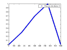
(a) $c_{ij}$ is unit conductance

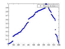
(b) $c_{ij}$ follows $U(0,1)$ distribution

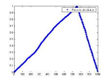
(c) $c_{ij}$ follows power-law distribution

Figure 1: Potential distribution on circles

From Figure 1, it is easy to see that there exist no concentration of potential distributions on circles no matter how we choose any distribution of conductance.

Case 2: $\mathbb{G}(n,p)$ model. We choose $G\in\mathbb{G}(n,p)$ with $n=1000$ , $p=0.01$ and the expected average degree is $10$. So $G$ is proper whp. Set the boundary potential as $V_{1}=1,V_{251}=0.3,V_{501}=0.7,V_{751}=1$. In Figure 2, we plot three pictures of potential distributions on $N=(G,c)$, where $c$ is unit conductance, unit $U(0,1)$ distribution, and power-law distribution (see[1]), respectively.

(a) $c_{ij}$ is unit conductance

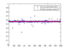
(b) $c_{ij}$ follows $U(0,1)$ distribution

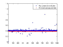
(c) $c_{ij}$ follows power-law distribution

Figure 2: Potential distribution on $\mathbb{G}(n,p)$ graphs

From Figure 2, it is easy to see that concentration of potential distribution appears when we choose unit conductance as we proved in Theorem 1.1, and we can use $\bar{V_{c}}$ as an efficient approximation of $V_{c}$. Even if the conductance follow certain distributions such that it approaches to $0$ or $+\infty$, we can still find concentration properties. But we are not able to give a rigorous mathematical proof in this case.
Case 3: The small world network. We choose $G$ to be a random graph $\mathbb{G}(n,p)$ adding to a circle of size $n$. Here we choose $n=1000$, $p=0.001$ so that $G$ may not be proper. Set the boundary potential as $V_{1}=1,V_{251}=0.3,V_{501}=0.7,V_{751}=1$. In Figure 3, we plot three pictures of potential distributions, where $c$ is unit conductance, unit $U(0,1)$ distribution, and power-law distribution (see[1]), respectively.

From Figure 3, it is easy to see that even if we choose the connecting probability $p$ very small, there also exists a concentration of potential distribution on small-world network except for a few vertices. We guess this is because the random walk on small-world network also has short mixing time as the random walk on $\mathbb{G}(n,p)$ model with large $p$ which we mentioned in equation (1).

It seems from the simulation results that only the structure of the electrical network will affect the concentration property. So we propose the following two questions:
Problem 4.1 Does the potential distribution for an electrical network $N=(G,c)$ concentrate where $G$ is proper and $c_{i,j}$ is i.i.d?
Problem 4.2 Does the potential distribution for a electrical network $N=(G,c)$ concentrate where $G$ is from small-world network with low connecting probability and $c_{i,j}$ is unit conductance or i.i.d as unit $U(0,1)$ or power-law distributions?

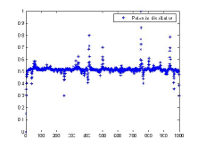
(a) $c_{ij}$ is unit conductance

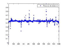
(b) $c_{ij}$ follows $U(0,1)$ distribution

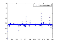
(c) $c_{ij}$ follows power-law distribution

Figure 3: Potential distribution on small-world networks

References

[1]A. L. Barabási, R. Albert, Emergence of scaling in random networks,
Science, 286(1999)509-512.
[2]B. Bollobás, Random Graphs 2nd ed., Cambridge
University Press, 2001.
[3]B. Bollobás, Modern Graph Theory. Springer-Verlag, New
York, 1998.
[4]
B. Bollobás, T. Fenner, and A. M. Frieze, An algorithm for
finding Hamilton paths and cycles in random graphs, Combinatorica 7(1987)327-341.
[5]
C. Cooper and A. Frieze, The cover time of sparse random graphs,
Random Structures and Algorithms, 30(2007)1-16.
[6]
E. B. Curtis and J. A. Morrow, The Dirichlet to Neumann map for a resistor
network, Journal on Applied Mathematics, 51(1991)1011-1029.
[7]P. G. Doyle and J. L. Snell, Random Walks
and Electronical Networks, Carus Math. Monogr., vol 22,
Mathematical Assoc. of America, Washington, 1984.
[8]
R. Durrett, Random Graph Dynamics, third ed., Cambridge
University Press, 2006.
[9]
D. Griffeath and T. M. Liggett, Critical phenomena for Spitzer s
reversible nearest particle systems, Ann. Probab.,
10(1982)881-895.
[10]
M. Jerrum and A. Sinclair, The Markov chain Monte Carlo
method:Anapproach to approximate counting and integration, In Approximation algorithms for NP-hard Problems, D. Hochbaum (Ed.),
PWS, Boston, MA, 1996, pp. 482-520.
[11]
S. Kakutani, Markov processes and the Dirichlet problem, Proc.
Jap. Acad., 21(1945)227-233.
[12]
F. Kelly, Reversibility and Stochastic Networks, Wiley,
Chichester, 1979.
[13]
J. G. Kemeny, J. L. Snell, and A. W. Knapp, Denumerable Markov
Chains, Van Nostrand, ? ? 1966.
[14]
H. Kesten, Percolation Theory for Mathematicians, ?? 1982.
[15]
T. J. Lyons, A simple criterion for transience of a reversible
Markov chain, Ann. Probab., 11(1983)393-402.
[16]R. Lyons and Y. Peres,
Probability on trees and networks, Preprint.
[17]J. L. Palacios, On hitting times of random walks on
trees, Statistics and Probability Letters, 79(2009)234-236.
[18]P. Tetali, Random walks and the effective resistance of
networks, Journal of Theoretical Probability, 4(1991)101-109.
[19]
D. J. Watts and S. H. Strogatz, Collective dynamics of small-world
networks, Nature, 393(1998)440-442.