Optimal Crowdsourcing Contests

Abstract

We study the design and approximation of optimal crowdsourcing contests. Crowdsourcing contests can be modeled as all-pay auctions because entrants must exert effort up-front to enter. Unlike all-pay auctions where a usual design objective would be to maximize revenue, in crowdsourcing contests, the principal only benefits from the submission with the highest quality. We give a theory for optimal crowdsourcing contests that mirrors the theory of optimal auction design: the optimal crowdsourcing contest is a virtual valuation optimizer (the virtual valuation function depends on the distribution of contestant skills and the number of contestants). We also compare crowdsourcing contests with more conventional means of procurement. In this comparison, crowdsourcing contests are relatively disadvantaged because the effort of losing contestants is wasted. Nonetheless, we show that crowdsourcing contests are 2-approximations to conventional methods for a large family of “regular” distributions, and $4$-approximations, otherwise.

1 Introduction

Crowdsourcing contests have become increasingly important and prevalent with the ubiquity of the Internet. For instance, instead of hiring a research team to develop a better collaborative filtering algorithm, Netflix issued the “Netflix challenge” offering a million dollars to the team that develops an algorithm that beats the Neflix algorithm by 10%. More generally, Taskcn allows users to post tasks with monetary rewards, collects submissions by other users, and rewards the best submission; and many Q&A sites allow users to post questions and reward the best answer with much-coveted “points”. We address two questions in this paper, (a) what format of crowdsourcing competition induces the highest-quality winning contribution, and (b) how inefficient is crowdsourcing over more conventional means of contracting.

Crowdsourcing competitions can be modeled as all-pay auctions. In the highest-bid-wins single-item all-pay auction, the auctioneer solicits payments (as bids), awards the item to the agent with the highest payment, and keeps all the agent payments. These auctions are well understood in settings where each agent has an independent private value for obtaining the item. In the connection to crowdsourcing contests, the “item” is the monetary reward, the payments are the submissions, and the private value is the rate at which the contestant works. However, unlike all-pay auctions, in crowdsourcing competitions the principal usually only values the winning submission and has no value for lesser submissions. Therefore, while the performance metric for auctions is usually revenue which is the sum of the agent payments, in crowdsourcing contests where payments are submissions, the relevant performance metric is the quality of the best submission, i.e., the maximum agent “payment”.

The revenue equivalence principle implies that in equilibrium the revenue of the highest-bid-wins all-pay auction is the same as that of first- and second-price auction formats; however, in these latter auction formats only the winner makes a payment. Since non-winners make payments in all-pay auctions, the maximum agent payment in all-pay auctions is lower than that of first- and second-price auctions. To connect this auction theory back to the setting of procurement, first- and second-price auctions are analogous to conventional procurement mechanisms, e.g., for government contracts, whereas the all-pay format is analogous to crowdsourcing contests. Importantly, the performance metric for first- and second-price procurement auctions is their revenue, that is, the winner’s payment. While the all-pay auction obtains the same total revenue, the principal in crowdsourcing cannot attain this full revenue and therefore suffers a loss relative to conventional methods.

Our first result is to show that in expectation the maximum agent payment in highest-bid-wins all-pay auctions is at least half its total revenue. Consequently crowdsourcing contests can extract from the best submission at least half of the total contribution from the crowd, which in turn implies that they are $2$-approximate with respect to conventional procurement via highest-bid-wins auctions. Of course, highest-bid-wins auctions are not necessarily revenue optimal. However, for a large class of distributions (termed regular), auctions that award the item to the highest bidder that meets a reservation price are optimal [Mye81]. In these settings crowdsourcing contests that require submissions to be of a minimum quality (e.g., the Netflix challenge required submissions to beat the Netflix algorithm by 10%) are $2$-approximations. For more general distributional settings reserve pricing gives a $2$-approximation to the optimal auction revenue [CHMS10] and crowdsourcing contests with minimum quality conditions are, therefore, $4$-approximations to conventional procurement. This approximation also implies a “simple versus optimal” style result, i.e., that the gains from precisely optimizing a contest based on the distribution versus running a simple highest-bid-wins crowdsourcing contest with a minimum quality condition are at most a factor of $4$.

Our second result derives the optimal static crowdsourcing format that maximizes the quality of the best submission. Specifically, suppose we fix the reward for the $k$-th best submission to be $a_{k}$ (where we normalize the $a_{k}$’s to $\sum_{k=1}^{n}a_{k}=1$). What should the $a_{k}$’s be? For instance on computer programming crowdsourcing site TopCoder.com, the best submission receives 2/3rds and the second-best submission receives 1/3rd of the total reward. Is this a better format than awarding the entire amount to the best submission in terms of the quality of that submission? We prove that it is not: $a_{1}=1$ and $a_{k}=0$ for $k>1$, or winner-takes-all, is the optimal choice over all such static contests.

Of course in some settings it may be better to adjust the number of rewards and their distribution across the participants dynamically as functions of the observed submission qualities. Our third result derives the format of crowdsourcing contests that dynamically optimizes the quality of the best submission. We give a complete characterization of optimal crowdsourcing contests. In what would be a familiar result to auction theorists, optimal crowdsourcing contests are “ironed virtual value optimizers” in that the reward is divided evenly among all contestants whose submissions are tied under a weakly monotone transformation (via the ironed virtual value function) of the submission quality. Importantly, the number of contestants who share the reward is determined dynamically and each contestant’s share is the same. Perhaps surprisingly, and unlike the case of classical auction theory, the transformation to ironed virtual values depends on the number of contestants.

Optimal crowdsourcing contests require the auctioneer to know the distribution of agents’ skills, e.g. in order to pick an appropriate minimum submission quality. In our fourth result we consider the loss from not knowing the distribution. For the revenue objective, Bulow and Klemperer [BK96] proved that for regular distributions recruiting an extra bidder is more profitable to the auctioneer than knowing the distribution. We show that this result implies that a simple highest-bid-wins contest approximates the optimal contest within a factor approaching $2$; this limits the benefit of knowing the skill distribution.

Related Work.

This paper follows the connection made between crowdsourcing contests and all-pay auctions from DiPalantino and Vojnovic [DV09] and questions from Archak and Sundararajan [AS09] and Moldovanu and Sela [MS01, MS06] on optimizing the reward structure to improve the quality of the best submissions. [AS09] and [MS01] compare winner-take-all crowdsourcing contests against ones with a statically determined division of the reward among top agents, e.g., as in the TopCoder.com mechanism. The objective in [MS01] is the sum of the qualities of submissions (analogous to revenue in our discussion) and the Archak-Sundararajan objective is the cumulative effort from the top $k$ agents less the monetary reward. Both papers show that when agents’ submission qualities are linear in their effort winner-take-all is optimal over other static divisions. The Moldovanu-Sela result also holds when quality is a convex function of effort, but not generally for concave functions. Minor [Min11] studies a generalization of the problem of Moldovanu and Sela, and derives the optimal crowdsourcing contest via a Myersonian ironing approach (again, to maximize the sum of qualities).

Moldovanu and Sela [MS06] study both the highest quality submission objective and the revenue (sum of all submission qualities) objective with the total reward normalized to 1. They compare the performance of two-stage contests against one-stage contests. Among one-stage contests they consider both a single grand contest, as well as many sub-contests in parallel, with the winner of each sub-contest receiving a prize. In two-stage contests, the winners of the first stage sub-contests compete in a final round. These are all static contests in the sense that the division of reward among winners of different sub-contests is predetermined. For the sum-of-qualities objective, [MS06] prove that a single grand contest is best among these contest formats. For the highest quality objective, if there are sufficiently many competitors then it is optimal to split the competitors in two divisions and to have a final among the two divisional winners. Further, as the number of competitors tends to infinity,  [MS06] show that the optimal highest quality objective is at least half of the optimal sum-of-qualities objective — we generalize this result and show that the factor of two ratio holds for any number of competitors.

In this paper our goal is to optimize the quality of the best submission (unlike [MS01, Min11] which consider total quality) with a total reward normalized to one (unlike [AS09] which optimizes the quality of the best submissions less the monetary reward). We study optimal crowdsourcing contests over all single-stage all-pay formats, unlike [MS06] which limits the format of one-stage contests but also studies two-stage contests. Our main results are to show that the wasted effort is not large and to characterize optimal crowdsourcing contests that can potentially divide the award between agents dynamically depending on the qualities of submissions. We also show that our model is consistent with that of [MS01, AS09] in that the optimal static allocation of the award is winner-take-all.

The following other results relating to crowdsourcing contests are technically unrelated to ours. DiPalantino and Vojnovic [DV09] study crowdsourcing websites as a matching market. They discuss equilibria where contestants first choose which contest to participate in and then their level of effort. Yang et al. [YAA08] and DiPalantino and Vojnovic [DV09] empirically study bidder behavior from crowdsourcing website Taskcn and conclude that experienced contestants strategize better than others and their strategizes match the BNE predictions fairly well.

There have been a number of studies of all-pay auctions in complete information settings (e.g., Baye et al. [BKdV96]), but these works are also technically unrelated to ours.

2 Preliminaries

Auction Theory.

Consider the standard auction-theoretic problem of selling a single item to $n$ agents. Each agent $i$ has a private value ${v_{i}}$ for receiving the object and is risk-neutral with linear utility ${u_{i}}={v_{i}}{x_{i}}-{p_{i}}$ for receiving the item with probability ${x_{i}}$ and making payment ${p_{i}}$. An auction ${\mathcal{A}}$ solicits bids and determines the outcome which consists of an allocation ${\mathbf{x}}=({x_{1}},\ldots,{x_{n}})$ and payments ${\mathbf{p}}=({p_{1}},\ldots,{p_{n}})$.

Suppose that the agents’ values are drawn i.i.d. from continuous distribution $F$ (that is, having no point-masses) with distribution function $F(z)=\text{\bf Pr}\!\left[{v_{i}}\leq z\right]$ and density function $f(z)$. A Bayes-Nash equilibrium (BNE) in auction ${\mathcal{A}}$ is a profile of strategies for mapping values to bids in the auction that are a mutual best response, i.e., when the values are drawn from $F$ and other agents follow their equilibrium strategies then each agent (weakly) prefers to also follow the prescribed strategy over taking any other action.

Formally, on valuation profile ${\mathbf{v}}=({v_{1}},\ldots,{v_{n}})$, denote the composition of an auction and a strategy profile by allocation rule ${\mathbf{x}}({\mathbf{v}})$ and payment rule ${\mathbf{p}}({\mathbf{v}})$. When agent $i$ is bidding in the auction, she knows her own value ${v_{i}}$ and assumes that the other agent values are drawn from the distribution $F$. Denote her interim allocation and payment rules as ${x_{i}}({v_{i}})=\text{\bf E}_{{\mathbf{v}}}\!\left[{x_{i}}({\mathbf{v}})\,\mid\,{v_{i}}\right]$ and ${p_{i}}({v_{i}})=\text{\bf E}_{{\mathbf{v}}}\!\left[{p_{i}}({\mathbf{v}})\,\mid\,{v_{i}}\right]$, respectively. Bayes-Nash equilibrium requires that ${v_{i}}{x_{i}}({v_{i}})-{p_{i}}({v_{i}})\geq{v_{i}}{x_{i}}(z)-{p_{i}}(z)$ for all $z$ and from this constraint is derived the standard characterization of BNE:

Theorem 2.1

[Mye81] Allocation and payment rules ${\mathbf{x}}(\cdot)$ and ${\mathbf{p}}(\cdot)$ are in BNE if and only if for all $i$

1. ${x_{i}}({v_{i}})$ is monotone non-decreasing in ${v_{i}}$ and

2. ${p_{i}}({v_{i}})={v_{i}}{x_{i}}({v_{i}})-\int_{0}^{{v_{i}}}{x_{i}}(z)dz+{p_{i}}(0)$

where usually ${p_{i}}(0)=0$.

A simple consequence of this characterization is the revenue equivalence principle which states that two mechanisms with the same equilibrium allocation have the same equilibrium revenue—in fact each agent’s expected interim payment is the same.

There are three standard formats for highest-bid-wins single-item auctions: first-price, second-price, and all-pay. In the first-price variant the highest bidder wins and pays her bid, in the second-price variant (a.k.a. the Vickrey auction) the highest bidder wins and pays the second highest bid, and in the all-pay variant the highest bidder wins and all bidders pay their bids. These auction formats all have BNE in which the agent with the highest valuation wins; Therefore, revenue equivalence implies that they have the same expected revenue (sum of payments) in equilibrium.

The highest-bid-win auction formats do not always yield the highest expected revenue. To solve for optimal auctions, Myerson [Mye81] defined virtual valuations for revenue as $\phi({v_{i}})={v_{i}}-\frac{1-F({v_{i}})}{f({v_{i}})}$ and proved that the expected payment of an agent, $\text{\bf E}_{{v_{i}}}\!\left[{p_{i}}({v_{i}})\right]$ is equal to her expected virtual value $\text{\bf E}_{{v_{i}}}\!\left[\phi({v_{i}}){x_{i}}({v_{i}})\right]$. The distribution $F$ is said to be regular if the virtual valuation function is monotone. For regular distributions, maximizing virtual values point-wise is a monotone allocation rule, and therefore can be implemented in BNE. The corresponding revenue-optimal auction serves the agent with the highest positive virtual value. By symmetry, this agent is identically the agent with the highest value that meets a reserve price of $\phi^{-1}(0)$.

Theorem 2.2

[Mye81] When the virtual valuation function $\phi(\cdot)$ is monotone, the optimal auction format is highest-bid-wins with a reservation value of $\phi^{-1}(0)$, a.k.a., the monopoly price.

It will be useful to be able to solve for the equilibrium strategies in all-pay auctions with reserves. Revenue equivalence makes this easy: the expected payment of an agent with value ${v_{i}}$ is the same in both the all-pay and the second-price auction formats. Of course in the all-pay format the agent always pays her bid; therefore, her bid $b({v_{i}})$ must be equal to her expected payment in the second-price auction. Let ${v_{(j)}}$ denote the $j$th largest value. Agent $i$’s expected payment in the second-price auction when ${v_{i}}\geq r$, is exactly $\text{\bf E}_{{\mathbf{v}}_{-i}}\!\left[\max({v_{(2)}},r)\,\mid\,{v_{i}}={v_{(1)}}\right]\text{\bf Pr}_{{\mathbf{v}}_{-i}}\!\left[{v_{i}}={v_{(1)}}\right]$, so her bid in the all-pay auction must be equal to this expectation.

Lemma 2.3

In a highest-bid-wins all-pay auction with value reserve $r$ an agent with value ${v_{i}}$ bids

$$b({v_{i}})=\text{\bf E}_{{\mathbf{v}}_{-i}}\!\left[\max({v_{(2)}},r)\,\mid\,{v_{i}}={v_{(1)}}\right]\text{\bf Pr}_{{\mathbf{v}}_{-i}}\!\left[{v_{i}}={v_{(1)}}\right].$$

if ${v_{i}}\geq r$ and $0$ otherwise.

The reserve specified above is in value-space. To implement such a reserve in an auction, one must translate it to a reserve in bid-space. For first- and second-price auctions this transformation is the identity function. For all-pay auctions, it can be calculated as follows. An agent with value equal to the reserve $r$ in the second price auction pays the reserve if she wins, i.e., her expected payment is $r\text{\bf Pr}_{{\mathbf{v}}_{-i}}\!\left[r={v_{(1)}}\right]=rF(r)^{n-1}$. By revenue equivalence the same agent in the equivalent all-pay auction must bid this expected payment; as this bid is the minimum bid that should be accepted, it is the reserve.

Lemma 2.4

The highest-bid-win all-pay auction with reserve bid $rF(r)^{n-1}$ implements the highest-value-wins allocation rule with a reserve value of $r$.

For irregular distributions, i.e., when $\phi(\cdot)$ is non-monotone, the revenue-optimal auction is not reserve-price based. Instead it selects the highest virtual value subject to monotonicity of the allocation rule. This optimization can be simplified by a very general ironing technique.

Theorem 2.5

[Mye81, HR08] There is an ironing procedure that converts any virtual valuation function $\phi(\cdot)$ to a ironed virtual valuation function $\bar{\phi}(\cdot)$ that is monotone and has the property that maximizing $\phi(\cdot)$ subject to monotonicity (of the allocation rule) is equivalent to maximizing $\bar{\phi}(\cdot)$ point-wise, with ties broken randomly. The BNE with this outcome is optimal.

Crowdsourcing.

The following model for crowdsourcing contests and its connection to all-pay auctions was proposed in [DV09]. To outsource a task to the crowd a principal announces a monetary reward (normalized to 1). Each of $n$ agents (the crowd) enters a submission. Agent $i$’s skill is denoted by ${v_{i}}$ and with effort, ${e_{i}}$, she can produce a submission with quality ${p_{i}}={v_{i}}{e_{i}}$, i.e., her skill can be thought of as a rate of work and her effort the amount of work. Each agent’s skill is her private information. If ${x_{i}}$ fraction of the reward is awarded to agent $i$ then her utility is ${u_{i}}={x_{i}}-{e_{i}}$. From her perspective ${v_{i}}$ is a constant so maximizing utility is equivalent to maximizing ${v_{i}}{u_{i}}={v_{i}}{x_{i}}-{p_{i}}$. Notice that this latter formulation of the agent’s objective mirrors that from the single-item auction setting discussed previously; furthermore, as the agents exert effort up-front, crowdsourcing contests intrinsically have all-pay semantics. Because of this connection, it will be convenient to refer interchangeably to contests as auctions, skills as values, submission qualities as payments, and rewards as allocations.

The objective for crowdsourcing contests ${\mathcal{A}}$ is to maximize the quality of the best submission. Because of the connection to all-pay auctions we refer to this objective as the maximum payment objective and denote its value for an auction ${\mathcal{A}}$ as ${\text{\bf MP}}[{\mathcal{A}}]=\text{\bf E}_{{\mathbf{v}}}\!\left[\max_{i}{p_{i}}({\mathbf{v}})\right]$. This objective is quite different from the standard revenue maximization objective ${\text{\bf Rev}}[{\mathcal{A}}]=\text{\bf E}_{{\mathbf{v}}}\!\left[\sum_{i}{p_{i}}({\mathbf{v}})\right]$.

One aim of this paper is to quantify the loss the principal incurs from running an all-pay auction versus a more conventional means of contracting. For instance, standard formats for procurement auctions are first- or second-price. Importantly, in first- and second-price auctions ${\mathcal{A}}$ all the payment comes from the highest bidder, therefore ${\text{\bf MP}}[{\mathcal{A}}]={\text{\bf Rev}}[{\mathcal{A}}]$ and the principal is able to extract quality workmanship with no loss. In contrast, in all-pay auctions which are revenue equivalent to first- and second-price auctions the maximum payment is not equal to the total revenue and thus the efforts of non-winners constitute a loss in performance. We thus quantify the utilization ratio of an auction ${\mathcal{A}}$ as $\frac{{\text{\bf Rev}}[{\mathcal{A}}]}{{\text{\bf MP}}[{\mathcal{A}}]}$.

We will see that the all-pay auction that optimizes maximum payment is not the same as the auction (all-pay or otherwise) that maximizes revenue. We define the approximation ratio of an all-pay auction to quantify its maximum payment relative to the revenue of the optimal (first-price or second-price) auction, i.e., ${\mathcal{A}}$’s approximation ratio is $\frac{{\text{\bf Rev}}[{\mbox{OPT}}]}{{\text{\bf MP}}[{\mathcal{A}}]}$. The cost of crowdsourcing (over conventional procurement) is then the approximation ratio of the best all-pay auction, i.e., $\inf_{{\mathcal{A}}}\frac{{\text{\bf Rev}}[{\mbox{OPT}}]}{{\text{\bf MP}}[{\mathcal{A}}]}$.

Non-zero density Assumption.

For the rest of this paper, the space of valuations $V$ is assumed to be an interval and the density function $f(\cdot)$ is assumed to be non-zero everywhere in $V$.

3 Utilization and approximation ratios

As noted previously, the maximum payment of a second- or first-price auction is equal to its total payment or revenue. On the other hand, in all-pay auctions the payment made by non-winners leads to a loss in performance. In this section we quantify this loss for a special class of all-pay auctions, namely those that always reward the highest bidder subject to an anonymous reserve price. This further allows us to find a simple all-pay auction that approximates optimal procurement.

In this section we consider highest-bidder-wins reserve-price auctions under either second-price or all-pay semantics. It is easy to see that under all-pay semantics these auctions induce symmetric continuous increasing bid functions at BNE and therefore their allocation function is identical to a second-price auction with an appropriate reserve price.

Theorem 3.1

Let ${\mathcal{A}}$ be any highest-bidder-wins reserve-price all-pay auction. Then ${\text{\bf Rev}}[{\mathcal{A}}]\leq 2{\text{\bf MP}}[{\mathcal{A}}]$. That is, its utilization ratio is bounded by $2$.

Proof: Let ${\mathbf{x}}$ denote the allocation function of the auction and suppose that the bid function that it induces in BNE is given by $b(v)$. We can write the expected revenue of the auction as the sum of the contribution from the winning agent (i.e. the agent with the maximum payment), and the contribution from other agents. Call the first term $A$ and the second $B$.

$${\text{\bf Rev}}[{\mathcal{A}}] =\underbrace{\sum_{i}\int_{v}b(v)\text{\bf Pr}_{{\mathbf{v}}_{-i}}\!\left[v={v_{(1)}}\right]f(v)\,dv}_{A}+\underbrace{\sum_{i}\int_{v}b(v)(1-\text{\bf Pr}_{{\mathbf{v}}_{-i}}\!\left[v={v_{(1)}}\right])f(v)\,dv}_{B}$$

Note that $A$ is precisely ${\text{\bf MP}}[{\mathcal{A}}]$. We will now show that $A\geq B$, or $A-B\geq 0$. By the revenue equivalence principle, $b(v)$ is equal to the expected payment that an agent with value $v$ makes in a second-price auction with the same allocation rule (Lemma 2.3). Let $g(v)$ denote the expected payment in the second-price auction with reserve, given that $v$ is the highest value. Then we get that $b(v)=g(v)\text{\bf Pr}_{{\mathbf{v}}_{-i}}\!\left[v={v_{(1)}}\right]$. We note that $\text{\bf Pr}_{{\mathbf{v}}_{-i}}\!\left[v={v_{(1)}}\right]=F(v)^{n-1}$ is a strictly increasing function since $f(v)\neq 0$ for all $v\in V$. Now we can write $A-B$ as

$$A-B =\sum_{i}\int_{v}b(v)(2\text{\bf Pr}_{{\mathbf{v}}_{-i}}\!\left[v={v_{(1)}}\right]-1)f(v)\,dv$$

$$=\sum_{i}\int_{v}g(v)F(v)^{n-1}(2F(v)^{n-1}-1)f(v)\,dv$$

$$=n\cdot\int_{v}g(F^{-1}(t))t^{n-1}(2t^{n-1}-1)\,dt$$

where, in the third equality, we substituted $t$ for $F(v)$.

Next we note that ignoring the $g$ term, the integral is non-negative:

$$\int_{0}^{1}t^{n-1}(2t^{n-1}-1)\,dt=\frac{2}{2n-1}-\frac{1}{n}>0$$

Let us consider the effect of the $g$ term. The function $t^{n-1}(2t^{n-1}-1)$ vanishes for two values of $t$ namely $0$ and $(1/2)^{\frac{1}{n-1}}$. Between these two values the function is negative, and for $t>(1/2)^{\frac{1}{n-1}}$, the function is positive. So when the function is multiplied by $g(F^{-1}(t))$, a non-decreasing function of $t$, the negative portion of the integral is magnified to a smaller extent than the positive portion, implying that the integral stays positive. This completes the proof.     

Tightness of Theorem 3.1.

We now exhibit an example where the utilization ratio of $2$ is tight. Consider a setting with $n$ agents, with each agent’s value distributed independently according to the $U[0,1]$ distribution. Consider the second-price auction with no reserve price. The expected revenue of this auction can be computed to be $\frac{n-1}{n+1}$. The corresponding all-pay auction induces a bid function $b(v)=\frac{n-1}{n}v^{n}$. The expected revenue of the all-pay auction is the same as that of the second-price auction, namely, $\frac{n-1}{n+1}$, which approaches $1$ as $n$ increases. On the other hand, the expected maximum payment can be computed to be $\frac{n-1}{2n}$ which approaches $1/2$ as $n$ increases. In Section 4 we will revisit this example and show that even the optimal all-pay auction (which is slightly better) only achieves an expected maximum payment approaching $1/2$ for this setting.

Utilization ratio for other all-pay auctions.

We note that the bound on utilization ratio does not hold for arbitrary symmetric all-pay auctions. For example, the all-pay auction corresponding to a revenue-optimal auction that requires ironing over large intervals of values induces a bidding function that is constant over those intervals. This results in many agents being tied for the reward, all making the same (low) payments but only one contributing to the maximum payment.

Approximation ratio.

Recall that the approximation ratio of an all-pay auction ${\mathcal{A}}$ is $\frac{{\text{\bf Rev}}[{\mbox{OPT}}]}{{\text{\bf MP}}[{\mathcal{A}}]}$, where OPT is the revenue optimal auction. We now use the bound on utilization ratio to prove that all-pay auctions achieve good approximation ratios. In particular, we note that for regular distributions highest-bidder-wins reserve-price auctions are revenue-optimal (Theorem 2.2). For irregular distributions, [CHMS10] show that highest-bidder-wins auctions with an anonymous reserve price are within a factor of $2$ of optimal. The following corollaries then follow from Theorem 3.1 upon applying the revenue equivalence principle.

Corollary 3.2

When agents’ value distributions are regular, there exists an $\alpha$ such that the highest-bid-wins all-pay auction with reserve bid $\alpha$ achieves an approximation ratio at most $2$.

Corollary 3.3

For all i.i.d. value distributions, there exists an $\alpha$ such that the highest-bid-wins all-pay auction with reserve bid $\alpha$ achieves an approximation ratio at most $4$.

These corollaries imply that the cost of crowdsourcing is always small — no more than $4$. The above example with uniform distributions shows that the approximation factor in Corollary 3.2 is tight. An extension of the same example in Section 4 shows that the worst-case cost of crowdsourcing can be no smaller than $2$.

4 Optimal crowdsourcing contests

In this section we characterize optimal crowdsourcing contests, first over a limited class of so-called “static” contests, and then over all contests.

Static Contests.

Consider the class of contests that predetermine the division of the reward into $a_{1},\dots a_{n}$, with $\sum_{i}a_{i}=1$. Agents are ordered by their submission qualities and awarded the corresponding fraction of reward, i.e., the $i$th best submission gets an $a_{i}$ fraction of the reward. Note that the Topcoder.com example mentioned in the introduction, where the best submission receives 2/3rds and the second-best submission receives 1/3rd of the total reward, falls under this class of contests. For this class, the following theorem shows that the optimal contest allocates the entire reward to the best submission; we defer the proof to Appendix A.

Theorem 4.1

When the bidders’ valuations are i.i.d., the optimal static all-pay auction is a highest-bid-wins auction.

Symmetric Contests.

For the rest of this section, we focus on the class of arbitrary symmetric contests. A symmetric auction is one where a permutation of bids results in the same permutation of the allocation and payments. Since agents’ private values are identically distributed, any such symmetric allocation rule induces a symmetric equilibrium in which all agents use an identical bidding function. This in turn implies that the allocation as a function of agents’ values is also symmetric across agents.

We first present a characterization of the expected maximum payment of any symmetric all-pay auction in terms of an appropriately defined virtual value function. This characterization immediately implies that the optimal mechanism is a virtual value maximizer.

Definition 1

For a given distribution $F$ with density function $f$ and an integer $n$, we define the virtual value for maximum payment, $\psi_{n}(z)$ as

$$\psi_{n}(z)=zF(z)^{n-1}-\frac{1-F(z)^{n}}{nf(z)}$$

Lemma 4.2

Consider a setting with $n$ agents and values distributed i.i.d. according to distribution $F$. Let ${\mathcal{A}}$ be a symmetric all-pay auction implementing the allocation function ${\mathbf{x}}$. Then ${\text{\bf MP}}[{\mathcal{A}}]=\text{\bf E}\!\left[\sum_{i}{x_{i}}({\mathbf{v}})\psi_{n}({v_{i}})\right]$.

Proof: Suppose that the allocation function ${\mathbf{x}}$ induces a symmetric bid function $b(\cdot)$ on the agents. Recall that by the revenue equivalence principle, $b(v)$ is equal to the expected payment that an agent with value $v$ makes under ${\mathbf{x}}(\cdot)$. From Theorem 2.1 we get the following expression for $b(v)$ where ${x_{i}}$ is the expected allocation to agent $i$ in expectation over ${\mathbf{v}}_{-i}$.

$$b({v_{i}})={v_{i}}{x_{i}}({v_{i}})-\int_{z=0}^{{v_{i}}}{x_{i}}(z)\,dz$$

Because the equilibrium is symmetric, one of the agents with the highest bid is the agent with the highest value, i.e., with ${v_{i}}={v_{(1)}}$. We attribute the maximum payment received by the mechanism to this agent. We can now use the above formulation of the bid function to calculate the expected contribution of agent $i$ to the maximum payment objective.

$${\text{\bf MP}_{i}}[{\mathcal{A}}] =\int_{{v_{i}}}b({v_{i}})\text{\bf Pr}_{{\mathbf{v}}_{-i}}\!\left[{v_{i}}={v_{(1)}}\right]f({v_{i}})\,d{v_{i}}$$

$$=\int_{{v_{i}}}\left[{v_{i}}{x_{i}}({v_{i}})-\int_{z=0}^{{v_{i}}}{x_{i}}(z)\,dz\right]F({v_{i}})^{n-1}{f_{i}}({v_{i}})\,d{v_{i}}$$

In order to simplify the second term in the integral we interchange the order of integration over $z$ and ${v_{i}}$, integrate over ${v_{i}}$, and then rename $z$ as ${v_{i}}$. We get:

$${\text{\bf MP}_{i}}[{\mathcal{A}}] =\int_{{v_{i}}}{v_{i}}{x_{i}}({v_{i}})F({v_{i}})^{n-1}{f_{i}}({v_{i}})\,d{v_{i}}-\int_{{v_{i}}}{x_{i}}({v_{i}})\left(\frac{1-F({v_{i}})^{n}}{n}\right)\,d{v_{i}}$$

$$=\int_{{v_{i}}}\left\{{v_{i}}F({v_{i}})^{n-1}-\frac{1-F({v_{i}})^{n}}{nf({v_{i}})}\right\}\times\,{x_{i}}({v_{i}}){f_{i}}({v_{i}})\,d{v_{i}}$$

$$=\int_{{v_{i}}}{x_{i}}({v_{i}})\psi_{n}({v_{i}}){f_{i}}({v_{i}})\,d{v_{i}}$$

$$=\text{\bf E}_{{\mathbf{v}}}\!\left[{x_{i}}({\mathbf{v}})\psi_{n}({v_{i}})\right]$$

Summing over $i$ implies the lemma.     

Optimal allocation rules and regularity.

The characterization of Lemma 4.2 immediately implies that in order to maximize the expected maximum payment, we should maximize the virtual surplus of the mechanism for maximum payment. In other words, we should allocate the entire reward to the agent that has the maximum virtual value $\psi_{n}({v_{i}})$ (subject to this value being non-negative). However, this results in a monotone allocation function only if the virtual value function is monotone non-decreasing. To this end, we define regularity for maximum payment as follows.

Definition 2

A distribution $F$ is said to be $n$-regular with respect to maximum payment if $\psi_{n}(\cdot)$ is a monotone non-decreasing function. The distribution is said to be regular w.r.t. maximum payment if $\psi_{n}(\cdot)$ is monotone non-decreasing for all positive integers $n$.

For distributions that are regular w.r.t. maximum payment, allocating to the agent with the highest non-negative virtual value is monotone and therefore can be implemented in BNE. Since agents have i.i.d. values, this outcome corresponds to allocating to the agent with the highest value, who is in turn the agent with the highest bid. Therefore, the optimal mechanism is a highest-bid-wins reserve-price mechanism. The reserve value for the mechanism is given by $\psi_{n}^{-1}(0)$ and the reserve bid can be computed by applying Lemma 2.4 to this value. We note that generally the reserve price is a function of $n$ and decreases with $n$, even for distributions that are regular for all $n$.

Theorem 4.3

Let $F$ be a distribution that is $n$-regular w.r.t. maximum payment. Then the optimal all-pay auction for $n$ agents with values distributed independently according to $F$ is a highest-bid-wins auction with a reserve price.

Two examples.

We now revisit the example with $n$ agents and values distributed according to $U[0,1]$ that was discussed in Section 3. The following expression defines the virtual value for maximum payment in this case:

$$\psi_{n}(z)=z^{n}(1+1/n)-1/n\,\,\text{ for }z\in[0,1]$$

This is an increasing function for all $n$. Therefore, the $U[0,1]$ distribution is regular. The optimal reserve value is given by $\psi_{n}^{-1}(0)=(n+1)^{-1/n}$, and the optimal reserve bid is $1/(n+1)$. Therefore, the optimal all-pay auction serves the highest bidder subject to her bid being at least $1/(n+1)$. The expected maximum payment of this auction can be calculated to be $\frac{n}{2(n+1)}$ which approaches $1/2$ as $n$ increases.

Next consider a setting with two agents and values distributed i.i.d. according to the exponential distribution. That is, $F(v)=1-e^{-v}$ for $v\geq 0$. We can calculate the virtual value function as $\psi_{2}(z)=(z-1)+e^{-z}(1/2-z)$. This function is negative below $1.21$ and positive thereafter. Furthermore, it is non-decreasing above $0.24$, particularly throughout the range where it is non-negative. So although the exponential distribution is not regular w.r.t. maximum payment, the optimal all-pay auction still turns out to be a highest-bid-wins auction with a reserve price of $1.21$ and a corresponding reserve bid of $0.85$.

An interesting point to note about the above example is that distributions that are regular with respect to the usual notion of virtual value for revenue, are not necessarily regular with respect to maximum payment even for $n=2$. However, for a large subset of such distributions, namely those that satisfy the monotone hazard rate condition (Definition 3 below), the optimal all-pay auction continues to have the simple form given in Theorem 4.3.

Regularity and MHR.

A common assumption in mechanism design literature is that value distributions satisfy the monotone hazard rate (MHR) condition defined below. Many common distributions such as the uniform, Gaussian, and exponential distributions satisfy this property. Distributions that satisfy MHR are regular and therefore do not require ironing in the context of revenue maximization. As our example above shows, MHR distributions are not necessarily regular with respect to maximum payment.

Definition 3

The hazard rate of a distribution $F$ with density function $f$ is defined as $h(x)=\frac{f(x)}{1-F(x)}$. A distribution is said to have a monotone hazard rate (MHR) if the hazard rate function is monotone non-decreasing.

Lemma 4.4

Let $F$ be a distribution satisfying the MHR condition. Then for any $n$ and any interval of values over which $\psi_{n}$ is non-negative, $\psi_{n}$ is monotone non-decreasing.

Proof: We can rewrite the virtual value function in terms of the hazard rate $h(z)$ of the distribution as follows.

$$\psi_{n}(z) =zF(z)^{n-1}-\frac{1}{nh(z)}\sum_{j=0}^{n-1}F(z)^{j}$$

$$=F(z)^{n-1}\left\{z-\frac{1}{nh(z)}\sum_{j=0}^{n-1}F(z)^{-j}\right\}$$

The function $h(z)$ is a non-negative non-decreasing function. Therefore, $(-1/nh(z))$ is a negative non-decreasing function. On the other hand, $\sum_{j=0}^{n-1}F(z)^{-j}$ is a decreasing function of $z$. The product of a negative non-decreasing function and a decreasing function is a non-decreasing function. Therefore, the term within brackets is a non-decreasing function of $z$. The term outside brackets, $F(z)^{n-1}$, is also an always positive increasing function. Therefore, the product of the two terms is an increasing function over any interval where it is positive.     

We obtain the following corollary.

Corollary 4.5

Let $F$ be a distribution that satisfies MHR. Then the optimal all-pay auction for values distributed independently according to $F$ is a highest-bid-wins auction with a reserve price.

Irregular distributions and ironing.

For distributions that are not regular according to the definition above, we can apply an ironing procedure from Theorem 2.5 to $\psi_{n}$ to obtain an ironed virtual value function $\overline{\psi}_{n}$. This function is monotone non-decreasing and by Theorem 2.5 the BNE that optimizes it point-wise optimizes the maximum payment objective.

The optimal mechanism in this case allocates the entire reward to the agent with the maximum ironed virtual value, in the case of ties distributing the reward equally among the tied agents. Since the ironed virtual value function is a weakly increasing function, the induced bid function is constant in the intervals where the ironed virtual value is constant, and discontinuous at the ends of those intervals. In effect, this creates intervals of bids that are suboptimal to make at any value; call these bid intervals “forbidden”. In order to implement the mechanism as an all-pay auction, we identify the forbidden bid intervals; then we round every bid in a forbidden bid interval down to the closest “allowed” bid, and distribute the reward equally among the highest bidders (subject to an appropriate reserve price defined by $(\overline{\psi}_{n})^{-1}(0)$). We therefore get the following theorem:

Theorem 4.6

For any setting with i.i.d. values, the optimal all-pay auction is defined by a reserve price and a subset of bids called forbidden bid intervals, that has the following format: the auction solicits bids and rounds them down to the nearest non-forbidden bids; it then distributes the reward equally among the highest bidders subject to the bids being above the reserve price.

An example of ironing.

We now present a simple example of a distribution that is irregular w.r.t. maximum payment, and derive its ironed virtual value and as well as forbidden bid intervals. There are two agents, each with a value drawn independently from $U[1,2]$ with probability $3/4$ and from $U[2,3]$ with probability $1/4$. Figure 1 below shows the virtual value function $\psi_{2}$ and its integral with respect to $q=F(v)$ using thick grey lines; their ironed counterparts are shown in thin red lines. The integral of the virtual value function as a function of $q$ is given by the expression $\frac{1}{2}F^{-1}(q)(1-q^{2})$. We iron this function by taking its convex envelope; $\overline{\psi}_{2}$ is then the derivative with respect to $q$ of that convex envelope.

The ironed virtual value is constant in the interval $[1.918,2.167]$. The probability of allocation (not plotted), and therefore the bid function, are also constant over this interval. The corresponding bid function is plotted with a thin black line below; there are two forbidden bid intervals, namely $[1.10,1.199)$ and $(1.199,1.31]$, with the intermediate value of $1.199$ being allowed. The two forbidden bid intervals correspond to the two discontinuities in the probability of allocation at the end points of the ironed interval.

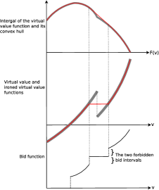
Figure 1: The Ironing Procedure

Irregularity as a function of $n$.

An interesting point to note is that irregularity increases with $n$. Specifically, the intervals of values that require ironing under $\psi_{n}$ increase with $n$. This does not necessarily imply that as $n$ increases a larger and larger number of agents are tied for the reward, for two reasons: (1) reserve value (not the reserve bid) could increase with $n$, and (2), due to the form of the virtual value function, ironing is typically necessary at low values rather than at high values.

Asymmetric contests.

We remark that even for symmetric instances (i.e. i.i.d. values) asymmetric all-pay auctions can be more powerful than symmetric all-pay auctions. We now present an example that exhibits this. Consider two contestants with values drawn i.i.d.  from $[0,1]$ according to the distribution $F(x)=x^{1.5}$. The optimal symmetric auction studied in this paper sets a reserve value of $(0.25)^{1/3}=0.63$ (which translates to a reserve bid of $(0.25)^{5/6}=0.315$) and serves the highest bidder who exceeds this reserve bid. This gives an expected maximum payment of $0.396$.

We now define a better auction that favors contestant 1 over contestant 2. The rules of the contest in value space are as follows. When contestant 1’s value is more than $0.75$ we serve him irrespective of contestant 2’s value, otherwise we serve the contestant with the higher value subject to a reserve value of $0.63$. This allocation rule creates a discontinuous increase in the expected allocation probability of player 1 at $0.75$, and hence a discontinuity in his bid function at $0.75$. In bid space, this corresponds to the following contest:

1. We set a reserve bid of $0.315$ as before.

2. All bids of contestant $1$ in the range $[0.418,0.681)$ get rounded down to $0.418$.

3. When contestant 1 bids at least $0.681$ he wins irrespective of 2’s bid.

4. Otherwise, the highest bidder wins with ties broken in favor of contestant 2.

By guaranteeing victory for contestant 1 beyond a certain bid, the above auction encourages contestant 1 to bid higher, thus boosting maximum payment. Since the objective is maximum payment, this type of bias is useful: the asymmetric auction obtains a smaller revenue but a larger expected maximum payment of $0.397$. We remark that in a real-world setting with a priori identical agents, favoring one agent over another may be socially unacceptable.

5 Prior-independent approximation

As we show above, optimal crowdsourcing contests depend on knowing the agents’ value distribution. To what extent is it important to know the distribution? In particular, under what conditions does the simple highest-bidder-wins contest without any reserve bid approximate the optimal one? We now show that for distributions that are regular w.r.t. revenue the simple highest-bidder-wins contest obtains an approximation ratio of $2n/(n-1)$, thus limiting the power of distributional knowledge.

For the standard goal of maximizing expected revenue, Bulow and Klemperer showed that for i.i.d. value distributions that are regular w.r.t. revenue, it is better to run a Vickrey auction with no reserve price on $n+1$ agents than to run an optimal auction on only $n$ agents. That is, the ability to recruit an extra agent in the auction is more profitable to the auctioneer than knowing the distribution.

We first note that Bulow and Klemperer’s result implies that for distributions that are regular w.r.t. revenue, the highest-value-wins auction with no reserve price on $n$ agents is within a factor of $(1-1/n)$ of the optimal mechanism in terms of revenue. This combined with Theorem 3.1 gives us the following theorem.

Theorem 5.1

For i.i.d. distributions that are regular w.r.t. revenue, the highest-bid-wins all-pay auction without a reserve bid obtains an approximation ratio of $2n/(n-1)$.

We remark that for the highest-value-wins auction without reserve prices, the revenue converges to the optimal as more and more agents are added. However for all-pay auctions adding more and more agents does not improve the approximation ratio beyond $2$.

Appendix A Proof of Theorem 4.1

Proof of Theorem 4.1. We begin by noting that the class of static auctions is symmetric, i.e., a permutation of bids results in the same permutation of the allocation and payments. Since agents’ private values are identically distributed, any such symmetric allocation rule induces a symmetric equilibrium in which all agents use an identical bidding function. This in turn implies that the allocation as a function of agents’ values is also symmetric across agents.

Let the agent values be distributed independently according to distribution function $F$, with density function $f$. Consider the static allocation rule ${\mathcal{A}}=(a_{1},\dots,a_{k},0,\dots,0)$, i.e, the agent with the $i$-th highest bid gets $a_{i}$ fraction of the reward if $i\leq k$, an 0 otherwise. We have $\sum_{i=1}^{k}a_{i}=1$. We focus on the symmetric bid-function $b(\cdot)$ induced by this allocation rule.

In a truthful auction with allocation rule ${\mathcal{A}}$, the expected payment made by the $r$-th highest bidder is $p_{r}(z)=\sum_{j=r+1}^{k+1}v_{jr}(z)(a_{j-1}-a_{j})$, where $v_{jr}(z)$ is the expectation of the $j$-th highest bid (=value) given the $r$-th highest bid is $z$.

Let $g(j,n,z)$ denote the expectation of the $j$-th highest draw among $n$ draws from $F$, given that the maximum draw is at most $z$. Then we have $v_{jr}(z)=g(j-r,n-r,z)$.

The contribution of bidder $i$ to the maximum payment objective is

$${\text{\bf MP}_{i}}[{\mathcal{A}}] =\int_{{v_{i}}}b({v_{i}})\text{\bf Pr}_{{\mathbf{v}}_{-i}}\!\left[{v_{i}}={v_{(1)}}\right]f({v_{i}})\,d{v_{i}}$$

$$=\int_{{v_{i}}}b({v_{i}})F({v_{i}})^{n-1}{f_{i}}({v_{i}})\,d{v_{i}}$$

Since agents values are drawn i.i.d. from $F$, we have ${\text{\bf MP}}[{\mathcal{A}}]=n{\text{\bf MP}_{i}}[{\mathcal{A}}]$.

Because the bid functions are symmetric, by the revenue equivalence principle, $b(z)$ equals the expected payment made by an agent with value $z$ in a truthful auction with the same allocation rule. So,

$$b(z) =\sum_{r=1}^{k}\text{\bf Pr}_{{\mathbf{v}}_{-i}}\!\left[z={v_{(r)}}\right]\cdot p_{r}(z)$$

$$=\sum_{r=1}^{k}\binom{n-1}{r-1}(1-F(z))^{r-1}F(z)^{n-r}\cdot\left\{\sum_{j=1}^{k+1-r}g(j,n-r,z)(a_{j+r-1}-a_{j+r})\right\}$$

We prove the theorem by showing that $\frac{d{\text{\bf MP}_{i}}[{\mathcal{A}}]}{da_{k}}$ is negative. When we change $a_{k}$ we assume that all the mass is transferred to (or drawn from) $a_{1}$. This will prove that the optimal allocation rule is to put all the mass on $a_{1}$, i.e., $a_{1}=1$.

Using the formula for $b(z)$, it is easy to observe that for $r=2$ to $r=k-1$, terms corresponding to that specific $r$ in $\frac{d{\text{\bf MP}_{i}}[{\mathcal{A}}]}{da_{k}}$ will be an integral with an integrand of

$$\binom{n-1}{r-1}(1-F(z))^{r-1}F(z)^{2n-r-1}\cdot\left\{-g(k-r,n-r,z)+g(k-r+1,n-r,z)\right\}$$

This integrand is negative because $g$ is a decreasing function in its first argument.

The term corresponding to $r=1$ in $\frac{d{\text{\bf MP}_{i}}[{\mathcal{A}}]}{da_{k}}$ will be an integral with an integrand of

$$F(z)^{2n-2}\cdot\left\{-g(1,n-1,z)-g(k-1,n-1,z)+g(k,n-1,z)\right\}$$

Note that the above integrand is negative even if $g(1,n-1,z)$ term were not there.

The term corresponding to $r=k$ in $\frac{d{\text{\bf MP}_{i}}[{\mathcal{A}}]}{da_{k}}$ will be an integral with a positive integrand of

$$\binom{n-1}{k-1}(1-F(z))^{k-1}F(z)^{2n-k-1}\cdot\left\{g(1,n-k,z)\right\}$$

Our proof is going to upper bound $\frac{d{\text{\bf MP}_{i}}[{\mathcal{A}}]}{da_{k}}$ by ignoring certain negative terms in it, and show that even the upper bound is negative. In particular, we only consider terms corresponding to $r=k-1$, $r=k$ and one term of $r=1$, namely $F(z)^{2n-2}\cdot\left\{-g(1,n-1,z)\right\}$. Let this upper bound be denoted by $Q$.

$$\frac{d{\text{\bf MP}_{i}}[{\mathcal{A}}]}{da_{k}}\leq Q =-\int_{z}F(z)^{2n-2}g(1,n-1,z)\,dF(z)$$

$$-\binom{n-1}{k-2}\int_{z}(1-F(z))^{k-2}F(z)^{2n-k}g(1,n-k+1,z)\,dF(z)$$

$$+\binom{n-1}{k-2}\int_{z}(1-F(z))^{k-2}F(z)^{2n-k}g(2,n-k+1,z)\,dF(z)$$

$$+\binom{n-1}{k-1}\int_{z}(1-F(z))^{k-1}F(z)^{2n-k-1}g(1,n-k,z)\,dF(z)$$

We derive the expressions for $g(1,n,z)$ and $g(2,n,z)$ below.

$$g(1,n,z) =n\int_{0}^{z}y\frac{f(y)}{F(z)}\left(\frac{F(y)}{F(z)}\right)^{n-1}\,dy$$

$$=z-\frac{\int_{0}^{z}F(t)^{n}\,dt}{F(z)^{n}}$$

$$g(2,n,z) =n(n-1)\int_{0}^{z}y\frac{f(y)}{F(z)}\left(1-\frac{F(y)}{F(z)}\right)\left(\frac{F(y)}{F(z)}\right)^{n-2}\,dy$$

$$=z-\left[n\frac{\int_{0}^{z}F(t)^{n-1}\,dt}{F(z)^{n-1}}-(n-1)\frac{\int_{0}^{z}F(t)^{n}\,dt}{F(z)^{n}}\right]$$

We susbtitute the expression for $g$ into $Q$.

$$Q =-\int_{z}F(z)^{n-2}\left[zF(z)^{n}-\int_{z}F(t)^{n}\,dt\right]\,dF(z)$$

$$+\binom{n-1}{k-1}\int_{z}(1-F(z))^{k-1}F(z)^{2n-k-1}z\,dF(z)$$

$$+\binom{n-1}{k-2}\int_{z}(1-F(z))^{k-2}F(z)^{n-1}\left(\int_{0}^{z}F(t)^{n-k+1}\,dt\right)\,dF(z)$$

$$+\binom{n-1}{k-2}(n-k)\int_{z}(1-F(z))^{k-2}F(z)^{n-1}\left(\int_{0}^{z}F(t)^{n-k+1}\,dt\right)\,dF(z)$$

$$-\binom{n-1}{k-2}(n-k+1)\int_{z}(1-F(z))^{k-2}F(z)^{n}\left(\int_{0}^{z}F(t)^{n-k}\,dt\right)\,dF(z)$$

$$-\binom{n-1}{k-1}\int_{z}(1-F(z))^{k-1}F(z)^{n-1}\left(\int_{0}^{z}F(t)^{n-k}\,dt\right)\,dF(z)$$

We now factor the term $(1-F(z))^{k-1}$ as $(1-F(z))^{k-2}\cdot(1-F(z))$ and then group terms. We get

$$Q =-\int_{z}F(z)^{n-2}\left[zF(z)^{n}-\int_{z}F(t)^{n}\,dt\right]\,dF(z)$$

$$-\binom{n-1}{k-1}\int_{z}(1-F(z))^{k-2}F(z)^{2n-k}z\,dF(z)$$

$$+\binom{n-1}{k-1}\int_{z}(1-F(z))^{k-2}F(z)^{2n-k-1}z\,dF(z)$$

$$+\binom{n-1}{k-2}(n-k+1)\int_{z}(1-F(z))^{k-2}F(z)^{n-1}\left(\int_{0}^{z}F(t)^{n-k+1}\,dt\right)\,dF(z)$$

$$-\binom{n-1}{k-2}\left[(n-k+1)-\frac{n-k+1}{k-1}\right]\int_{z}(1-F(z))^{k-2}F(z)^{n}\left(\int_{0}^{z}F(t)^{n-k}\,dt\right)\,dF(z)$$

$$-\binom{n-1}{k-1}\int_{z}(1-F(z))^{k-2}F(z)^{n-1}\left(\int_{0}^{z}F(t)^{n-k}\,dt\right)\,dF(z)$$

We have to prove that $Q\leq 0$. This is equivalent to proving that

$$\int_{z}F(z)^{n-2}\left[zF(z)^{n}-\int_{0}^{z}F(t)^{n}\,dt\right]\,dF(z)$$

$$+\binom{n-1}{k-1}\int_{z}(1-F(z))^{k-2}F(z)^{n-1}\left[zF(z)^{n-k+1}-\int_{0}^{z}F(t)^{n-k+1}\,dt\right]\,dF(z)$$

$$-\binom{n-1}{k-1}\int_{z}(1-F(z))^{k-2}F(z)^{n-1}\left[zF(z)^{n-k}-\int_{0}^{z}F(t)^{n-k}\,dt\right]\,dF(z)$$

$$\geq$$

$$\binom{n-1}{k-1}(k-2)\int_{z}(1-F(z))^{k-2}F(z)^{n-1}\left(\int_{0}^{z}F(t)^{n-k+1}\,dt\right)\,dF(z)$$

$$-\binom{n-1}{k-1}(k-2)\int_{z}(1-F(z))^{k-2}F(z)^{n}\left(\int_{0}^{z}F(t)^{n-k}\,dt\right)\,dF(z)$$

The RHS can be seen to be negative. Thus it is enough to prove that the LHS is positive. Rewriting the terms in the square bracket via integration by parts,

$$n\int_{z}F(z)^{n-2}\left(\int_{0}^{z}tF(t)^{n-1}\,dF(t)\right)\,dF(z)$$

$$+\binom{n-1}{k-1}(n-k+1)\int_{z}(1-F(z))^{k-2}F(z)^{n-1}\left(\int_{0}^{z}tF(t)^{n-k}\,dF(t)\right)\,dF(z)$$

$$-\binom{n-1}{k-1}(n-k)\int_{z}(1-F(z))^{k-2}F(z)^{n-1}\left(\int_{0}^{z}tF(t)^{n-k-1}\,dF(t)\right)\,dF(z)$$

Changing the order of integration, we have the LHS as,

$$\int_{t=0}^{\infty}tF(t)^{n-k-1}f(t)\left\{\begin{split}\binom{n-1}{k-1}(n-k+1)\left(\int_{F(t)}^{1}(1-F(z))^{k-2}F(z)^{n-1}\,dF(z)\right)\left[F(t)-\frac{n-k}{n-k+1}\right]\qquad\\ \qquad+n\left(\int_{F(t)}^{1}F(z)^{n-2}\,dF(z)\right)F(t)^{k}\end{split}\right\}\,dt$$

Applying integration by parts again, (this time taking $t$ as one term and the rest as the differential part) we get the LHS as,

$$\int_{t=0}^{\infty}\left(\int_{F(t)}^{1}u^{n-k-1}\left\{\begin{split}\binom{n-1}{k-1}(n-k+1)\left(\int_{u}^{1}(1-F(z))^{k-2}F(z)^{n-1}\,dF(z)\right)\left[u-\frac{n-k}{n-k+1}\right]\qquad\\ \qquad+n\left(\int_{u}^{1}F(z)^{n-2}\,dF(z)\right)u^{k}\end{split}\right\}\,du\right)\,dt$$

Rewrite the above integral as $\int_{t=0}^{\infty}H_{n}(F(t))\,dt$ where

$$H_{n}(x)=\int_{x}^{1}u^{n-k-1}\left\{\binom{n-1}{k-1}(n-k+1)\left(\int_{u}^{1}(1-v)^{k-2}v^{n-1}\,dv\right)\left[u-\frac{n-k}{n-k+1}\right]+n\left(\int_{u}^{1}v^{n-2}\,dv\right)u^{k}\right\}\,du$$

If we prove that $H_{n}(x)$ is always non-negative for $x\in[0,1]$ we are done. We have

$$-H_{n}^{\prime}(x)=x^{n-k-1}\left\{\binom{n-1}{k-1}(n-k+1)\left(\int_{x}^{1}(1-v)^{k-2}v^{n-1}\,dv\right)\left[x-\frac{n-k}{n-k+1}\right]+n\left(\int_{x}^{1}v^{n-2}\,dv\right)x^{k}\right\}$$

Observe that $-H_{n}^{\prime}(x)$ is negative for small values of $x$ and positive for large values of $x$ and never becomes negative after it has become positive. Thus, $H_{n}(x)$ is first increasing and then decreasing. We know that $H_{n}(1)=0$. If we prove that $H_{n}(0)\geq 0$, we would have proven that $H_{n}(x)$ is always non-negative.

$$H_{n}(0) =\binom{n-1}{k-1}(n-k+1)\int_{0}^{1}u^{n-k-1}\left(\int_{u}^{1}(1-v)^{k-2}v^{n-1}\,dv\right)\left[u-\frac{n-k}{n-k+1}\right]\,du$$

$$+n\int_{0}^{1}\left(\int_{u}^{1}v^{n-2}\,dv\right)u^{n-1}\,du$$

$$=\binom{n-1}{k-1}(n-k+1)\int_{0}^{1}(1-v)^{k-2}v^{n-1}\left(\int_{0}^{v}u^{n-k-1}\left[u-\frac{n-k}{n-k+1}\right]\,du\right)\,dv$$

$$+n\int_{0}^{1}v^{n-2}\left(\int_{0}^{v}u^{n-1}\,du\right)\,dv$$

$$=\binom{n-1}{k-1}\int_{0}^{1}(1-v)^{k-2}v^{2n-k-1}(v-1)\,dv+\frac{1}{2n-1}$$

$$=-2\binom{n-1}{k-1}\int_{0}^{\pi/2}cos^{4n-2k-1}(\theta)sin^{2k-1}(\theta)\,d\theta+\frac{1}{2n-1}$$

The integral $\int_{0}^{\pi/2}cos^{m}(\theta)sin^{n}(\theta)\,d\theta=\frac{\Gamma(\frac{m+1}{2})\Gamma(\frac{n+1}{2})}{2\Gamma(\frac{m+n+2}{2})}$ Accordingly, we have

$$H_{n}(0) =-\binom{n-1}{k-1}\frac{\Gamma(2n-k)\Gamma(k)}{\Gamma(2n)}+\frac{1}{2n-1}$$

$$>0$$

References

- [AS09] Nikolay Archak and Arun Sundararajan. Optimal design of crowdsourcing contests. In International Conference on Information Systems (ICIS), 2009.
- [BK96] J. Bulow and P. Klemperer. Auctions versus negotiations. American Economic Review, 86:180–194, 1996.
- [BKdV96] Michael R. Baye, Dan Kovenock, and Casper G. de Vries. The all-pay auction with complete information. Economic Theory, 8:291–305, 1996. 10.1007/BF01211819.
- [CHMS10] Shuchi Chawla, Jason D. Hartline, David L. Malec, and Balasubramanian Sivan. Multi-parameter mechanism design and sequential posted pricing. In Proceedings of the 42nd ACM symposium on Theory of computing, STOC ’10, pages 311–320, New York, NY, USA, 2010. ACM.
- [DV09] Dominic DiPalantino and Milan Vojnovic. Crowdsourcing and all-pay auctions. In Proceedings of the 10th ACM conference on Electronic commerce, EC ’09, pages 119–128, New York, NY, USA, 2009. ACM.
- [HR08] Jason D. Hartline and Tim Roughgarden. Optimal mechanism design and money burning. In Proceedings of the 40th annual ACM symposium on Theory of computing, STOC ’08, pages 75–84, New York, NY, USA, 2008. ACM.
- [Min11] Dylan Minor. Increasing efforts through rewarding the best less. Mansucript, 2011.
- [MS01] Benny Moldovanu and Aner Sela. The optimal allocation of prizes in contests. American Economic Review, 91(3):542–558, 2001.
- [MS06] Benny Moldovanu and Aner Sela. Contest architecture. Journal of Economic Theory, 126(1):70–97, 2006.
- [Mye81] R. Myerson. Optimal auction design. Mathematics of Operations Research, 6:58–73, 1981.
- [YAA08] Jiang Yang, Lada A. Adamic, and Mark S. Ackerman. Crowdsourcing and knowledge sharing: strategic user behavior on taskcn. In Proceedings of the 9th ACM conference on Electronic commerce, EC ’08, pages 246–255, New York, NY, USA, 2008. ACM.