Bond order solid of two-dimensional dipolar fermions

Abstract

Recent experimental realization of dipolar Fermi gases near or below quantum degeneracy provides opportunity to engineer Hubbard-like models with long range interactions. Motivated by these experiments, we chart out the theoretical phase diagram of interacting dipolar fermions on the square lattice at zero temperature and half filling. We show that in addition to $p$-wave superfluid and charge density wave order, two new and exotic types of bond order emerge generically in dipolar fermion systems. These phases feature homogeneous density but periodic modulations of the kinetic hopping energy between nearest or next-nearest neighbors. Similar, but manifestly different, phases of two-dimensional correlated electrons have previously only been hypothesized and termed “density waves of nonzero angular momentum”. Our results suggest that these phases can be constructed flexibly with dipolar fermions, using currently available experimental techniques.

Experimental demonstration of Bose-Einstein condensation of atomic chromium chromium and dysprosium benlev , both of which have large magnetic dipole moments, ushers the ultra-cold dipolar gas to the arena of quantum emulation simu ; rey . A gas of the fermionic isotope of dysprosium, ¹⁶¹Dy, has been cooled below quantum degeneracy priv . A high space-density gas of ⁴⁰K⁸⁷Rb, fermionic molecules with electric dipole moments, has recently been produced near quantum degeneracy jun1 and confined in optical lattice op-la . Such systems are expected to show a rich array of quantum phases arising from the long-range and anisotropic nature of dipole-dipole interaction baranov1 ; lahaye ; fradkin . This uniquely distinguishes the dipolar Fermi gas from other Fermi systems, e.g. the 2D electron gas, the quantum fluid of ³He, and Fermi gases of alkali atoms with short range interactions.

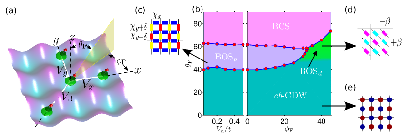
Figure 1: (Color online) Dipolar fermions on square lattice. (a) Schematic of the dipolar fermions confined to a square optical lattice potential. The induced dipole moment ${\bf d}$ points along the direction $\hat{d}=\cos\theta_{\text{F}}\hat{z}+\sin\theta_{\text{F}}\cos\phi_{\text{F}}\hat{x}+\sin\theta_{\text{F}}\sin\phi_{\text{F}}\hat{y}$. (b)Phase diagram obtained via FRG indicating four phases: $p$-wave bond order solid (BOS_p), $d$-wave bond order solid (BOS_d), checkerboard charge density wave ($cb$-CDW), and $p$-wave BCS superfluid (BCS); left panel– phase diagram in the $\theta_{\text{F}}$-$V_{\text{d}}$ plane at $\phi_{\text{F}}=0$; right panel– phase diagram in the $\theta_{\text{F}}$-$\phi_{\text{F}}$ plane at $V_{\text{d}}=0.5t$. The phase boundary (solid line) is determined by the abrupt change in the symmetry of the eigenvector of the dominant instability (see Fig. 2). The smooth crossover from $cb$-CDW and BOS_d is indicated by a gradual change of the color shading. (c)-(e) Schematic of the bond or density modulation pattern for the BOS_p, BOS_d, and $cb$-CDW phase respectively.

Previous works on dipolar Fermi gases have investigated the anisotropic Fermi liquid properties fradkin ; congjun2 , the pairing instability baranov2 ; baranov3 ; taylor ; cooper1 ; hanpu , phases showing density modulation miyakawa ; freericks , as well as liquid crystal states quin ; congjun1 ; erhai . The possibility of supersolid phases hofstetter has also been discussed.

For a 2D dipolar Fermi gas on a square lattice at half filling, with dipole moments perpendicular to the plane, one expects to find a checkerboard density modulation, known as the charge density wave (CDW, we follow the nomenclature even though atoms/molecules are charge neutral). When the dipole moments are aligned in the lattice plane the system becomes an anisotropic superfluid and the attractive interaction binds fermions into Cooper pairs. The main question we address here is, how do different orders compete or cooperate as the dipole moments are turned from perpendicular to parallel orientation?

We employ the functional renormalization group (FRG) technique shankar ; zanchi ; mathey , along with self consistent mean field (SCMF) ripka to obtain, for the first time, the zero-temperature phase diagram of dipolar fermions on a two dimensional lattice at half filling. The FRG takes an unbiased approach to treat all the instabilities of the Fermi surface, revealing the existence of two new and fascinating quantum phases: the $p$-wave bond order solid (BOS_p); and the $d$-wave bond order solid (BOS_d). These bond order solids may be considered as 2D analogues of the “bond order wave” found in the 1D extended Hubbard model nakamura ; pinaki ; shan-wen1 .

We model single-component dipolar fermions on a two-dimensional square lattice with lattice constant $a_{\text{L}}$ by the Hamiltonian

$$H=-t\sum_{\langle ij\rangle}a_{i}^{\dagger}a_{j}+\frac{1}{2}\sum_{i\neq j}V_{ij}n_{i}n_{j},$$ (1)

where $t$ represents the nearest neighbor hopping, $a_{i}$ is the fermion annihilation operator at the site $i$, $n_{i}=a_{i}^{\dagger}a_{i}$ is the number operator. The site index $i$ represents a lattice site centered at $\mathbf{r}_{i}=i_{x}a_{\text{L}}\hat{x}+i_{y}a_{\text{L}}\hat{y}$, where $i_{x}$, $i_{y}$ are integers. The matrix elements of the dipole interaction in the two-particle Wannier basis are given by $V_{ij}=\langle ij|V_{\text{dd}}|ij\rangle=V_{\text{d}}[1-3(\hat{r}_{ij}\cdot\hat{d})^{2}]/{(r_{ij}/a_{\text{L}})^{3}}$, where $\mathbf{r}_{ij}\equiv\mathbf{r}_{i}-\mathbf{r}_{j}$ and the dipoles are pointing in the same direction $\hat{d}$. We assume an external electric or magnetic field ${\bf F}$ pointing in some general direction. Then the interaction energy of the dipole moment ${\bf d}$ with the field ${\bf F}$ is equal to $-{\bf F}\cdot{\bf d}$, implying that the orientation of the dipole moments can be tuned by ${\bf F}$. We label the direction of ${\bf d}$ by polar and azimuthal angles $\theta_{\text{F}}$ and $\phi_{\text{F}}$ respectively, as illustrated in the schematic of Fig. 1(a).

The interaction between dipoles can be attractive or repulsive depending on $\theta_{\text{F}}$, $\phi_{\text{F}}$ and $\mathbf{r}_{ij}$. For example [refer to Fig. 1(a)], if $\phi_{\text{F}}=0$, $V_{y}\equiv V_{\text{dd}}(a_{\text{L}}\hat{y})$ is always repulsive, while $V_{x}\equiv V_{\text{dd}}(a_{\text{L}}\hat{x})$ and $V_{3}\equiv V_{\text{dd}}(a_{\text{L}}\hat{x}+a_{\text{L}}\hat{y})$ become negative for $\theta_{\text{F}}>\vartheta_{\text{c1}}\approx 35.26^{\circ}$ and $\theta_{\text{F}}>\vartheta_{\text{c2}}=\cos^{-1}(1/\sqrt{3})\approx 54.74^{\circ}$ respectively. We shall show that these two critical points, $\vartheta_{\text{c1}}$ and $\vartheta_{\text{c2}}$, roughly set the phase boundary between the checkerboard charge density wave ($cb$-CDW), BOS_p, and the Bardeen-Cooper-Schrieffer (BCS) superfluid phase, for the $\phi_{\text{F}}=0$ case.

We now discuss the $T=0$ phase diagram at half filling. First, we analyze the weakly interacting limit, $V_{\text{d}}<t$, using FRG. In this approach, no assumptions about possible dominant orders are necessary. Rather, the method includes all processes near the Fermi surface of the non-interacting system via the generalized 4-point vertex function: $U_{\ell}({\bf k}_{1},{\bf k}_{2},{\bf k}_{3})$, where ${\bf k}_{1,2}$ (${\bf k}_{3,4}$) are incoming (outgoing) momenta and ${\bf k}_{4}={\bf k}_{1}+{\bf k}_{2}-{\bf k}_{3}$. Here, $\ell$ is the renormalization group flow parameter that relates the energy cutoff $\Lambda$ to the initial cutoff $\Lambda_{0}$ (chosen to be $4t$) via $\Lambda_{\ell}=\Lambda_{0}e^{-\ell}$. Starting with the bare vertex $U_{0}$, progressively tracing out the high energy degrees of freedom, a set of coupled integro-differential equations give the FRG flow for all the vertices.

The renormalized vertex for specific channels of interest, e.g.,

$$\left.\begin{array}[]{l}U^{\text{NEST}}_{\ell}({\bf k}_{1},{\bf k}_{2})=U_{\ell}({\bf k}_{1},{\bf k}_{2},{\bf k}_{1}+{\bf Q}),\\ U^{\text{BCS}}_{\ell}({\bf k}_{1},{\bf k}_{2})=U_{\ell}({\bf k}_{1},-{\bf k}_{1},{\bf k}_{2}),\end{array}\right\}$$ (2)

are extracted by appropriately constraining the in-coming and out-going momenta. Here ${\bf Q}=(\pi,\pm\pi)$ is the nesting vector at half filling for the square lattice, and $U_{\ell}^{\text{NEST}}$ is the same as $U_{\ell}^{\text{CDW}}$ of Ref. zanchi . The channel matrix with the largest divergent eigenvalue $\lambda$ corresponds to the most dominant instability of the Fermi liquid. The corresponding eigenvector $\psi$ defined on the Fermi surface, indicates the symmetry of the incipient order parameter associated with the instability.

We perform the FRG analysis for a range of values of $V_{\text{d}}$, $\theta_{\text{F}}$, and $\phi_{\text{F}}$ producing a 3D phase diagram, visualized in Fig. 1(b) as slice cuts along two different planes. To capture and emphasize the key elements of the phase diagram, first we fix $\phi_{\text{F}}=0$, generating a 2D phase diagram in the $\theta_{\text{F}}$–$V_{\text{d}}$ plane shown in the left panel of Fig. 1(b). Next we fix $V_{\text{d}}=0.5t$ instead, yielding the $\theta_{\text{F}}$–$\phi_{\text{F}}$ plane shown in the right panel of Fig. 1(b).

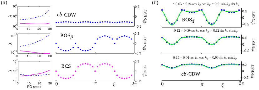
Figure 2: (Color online) FRG results for $V_{\text{d}}=0.5t$. The FRG is implemented numerically by discretizing the Fermi surface into 32 patches distributed at equally spaced angular points. (a) Top, middle and bottom panels represent FRG results for $(\theta_{\text{F}},\phi_{\text{F}})=(30^{\circ},0),(42^{\circ},0)$ and $(70^{\circ},0)$ respectively. Left column: the largest eigenvalue $\lambda$ of the NEST (dashed line) and BCS (solid line) channel. Right column: the corresponding eigenvector $\psi$ of the most diverging channel as function of $\xi$, the angle of the discrete $\bf{k}$ points on the Fermi surface defined by $\tan\xi=k_{y}/k_{x}$, plotted with square markers. (b) Top, middle and bottom panel represent FRG results for $(\theta_{\text{F}},\phi_{\text{F}})=(62^{\circ},40^{\circ}),(46^{\circ},40^{\circ})$ and $(38^{\circ},40^{\circ})$ plotted using square markers. The fit is shown in solid line. As $\theta_{\text{F}}$ is increased, $\psi$ smoothly changes from nodeless for $\theta_{\text{F}}\lessapprox 46^{\circ}$ to one with nodes for $\theta_{\text{F}}\gtrapprox 46^{\circ}$.

The $\theta_{\text{F}}$–$V_{\text{d}}$ phase diagram shows the existence of three phases separated by two critical angles $\theta_{\text{F}}=\theta_{1}$ and $\theta_{2}$, with no appreciable dependence on $V_{\text{d}}$. For $0\leq\theta_{\text{F}}<\theta_{1}$, the nesting channel has the largest (most divergent) eigenvalue $\lambda$. The corresponding eigenvector $\psi_{\text{NEST}}$, as illustrated in top panel of Fig. 2(a), is almost constant with only small modulation along the Fermi surface. This implies the onset of CDW order with $s$-wave symmetry, identified as a checkerboard modulation of on-site density, the $cb$-CDW shown in Fig. 1(e). The physical origin of this phase can be traced by observing that $\theta_{1}\approx\vartheta_{1\text{c}}$, thus $V_{x},V_{y},V_{3}>0$ in this regime, allowing for a low energy configuration with density concentrated on the next-to-nearest neighbor sites, consistent with the perfect nesting of the Fermi surface. For $\theta_{2}\leq\theta_{\text{F}}\leq 90^{\circ}$, the BCS channel exhibiting a $p$-wave symmetry is the most diverging under FRG flow [see Fig. 2(a)]. In real space, this corresponds to the onset of nearest neighbor pairing, $\langle a_{i}a_{i+\hat{x}}\rangle=-\langle a_{i}a_{i-\hat{x}}\rangle$ generated by couplings $V_{x}$ and $V_{3}$, both becoming attractive for $\theta_{\text{F}}>\theta_{2}\sim\vartheta_{2\text{c}}$. The superfluid phase here is the lattice analog of the $p$-wave BCS phase discussed previously for continuum dipolar Fermi gases baranov1 ; taylor ; hanpu .

Finally the intermediate regime, $\theta_{1}\leq\theta_{\text{F}}<\theta_{2}$, is the most intriguing. The FRG predicts a leading instability in the nesting channel, similar to the $cb$-CDW, but instead with a $p$-wave symmetry, $\psi_{\text{NEST}}({\bf k})\sim\chi({\bf k})=\chi_{0}\sin k_{y}$, as shown in middle panel of Fig. 2(a). This result suggests a broken symmetry phase, shown in Fig. 1(c), with periodic modulation of $\langle a^{\dagger}_{i}a_{i+\hat{y}}-\chi_{y}\rangle=-\langle a^{\dagger}_{i}a_{i-\hat{y}}-\chi_{y}\rangle=\delta(-1)^{i_{x}+i_{y}}$, where $\chi_{y}$ is average of $\langle a^{\dagger}_{i}a_{i+\hat{y}}\rangle$ over all bonds. We observe that the nesting vector ${\bf Q}$ is consistent with the checkerboard pattern of bond variable representing nearest-neighbor hopping. We refer to this broken symmetry phase as the $p$-wave bond order solid (BOS_p). Phases with similar, but manifestly different bond order patterns were conjectured by Nayak and referred to as $p$-density waves nayak .

The right panel of Fig. 1(b), $\theta_{\text{F}}$–$\phi_{\text{F}}$ phase diagram at fixed interaction strength, $V_{\text{d}}=0.5t$, shows the three phases above for small values of $\phi_{\text{F}}$. However, as $\phi_{\text{F}}$ is increased towards $45^{\circ}$, the BOS_p region shrinks and eventually disappears beyond $\phi_{\text{F}}\sim 35^{\circ}$. Such change is due to the new features in the dipolar interactions for $\phi_{\text{F}}$ close to $45^{\circ}$, where $V_{x}\sim V_{y}$, but the next-to-nearest neighbor interaction along $\hat{x}+\hat{y}$ and $\hat{x}-\hat{y}$ develop opposite sign. We find that for such large values of $\phi_{\text{F}}\sim 45^{\circ}$, the eigenvector can be fit very well by $\psi_{\text{NEST}}({\bf k})=\alpha+\beta[\cos k_{x}\cos k_{y}+\sin k_{x}\sin k_{y}]$, as seen in the right panel of Fig. 2(b). As $\theta_{\text{F}}$ is increased, the constant term $\alpha$, which describes the density modulation of $cb$-CDW order, is gradually reduced, while the magnitude of $\beta$ increases. In the green shaded region in Fig. 1(b), $\alpha/\beta$ drops gradually from 1 to 0 as $\theta_{F}$ is increased toward the phase boundary to BCS. We refer to this region where the $\cos k_{x}\cos k_{y}$ and $\sin k_{x}\sin k_{y}$ components of $\psi_{\text{NEST}}$ dominant as the $d$-wave bond order solid (BOS_d). In this phase, the density and the nearest hopping $\langle a^{\dagger}_{i}a_{i+\hat{x}/\hat{y}}\rangle$ are homogeneous. But the dipolar interaction induces an effective diagonal hopping, $\langle a^{\dagger}_{i}a_{i-\hat{x}+\hat{y}}\rangle$, a bond variable with amplitude proportional to $\beta$ and spatial pattern shown schematically in Fig. 1(d). BOS_d found here differs from the $d_{xy}$-density wave conjectured in Ref. nayak .

To firmly pin down the nature of the phases, we complement the FRG analysis with SCMF theory (see Ref. ripka ) on a square lattice of finite size $L\times L$ with period boundary condition by defining the normal and pair density matrices $\rho_{ij}=\langle a_{j}^{\dagger}a_{i}\rangle$ and $m_{ij}=\langle a_{i}a_{j}\rangle$ respectively. The corresponding mean fields are then given by $\chi_{ji}=-\sum_{kl}\langle jk|V_{\text{dd}}|li\rangle\rho_{lk}$ and $\Delta_{ij}=-\frac{1}{2}\sum_{kl}\langle ij|V_{\text{dd}}|kl\rangle m_{lk}$. The dipole interaction is retained up to a distance of $10a_{\text{L}}$. We search for the ground state iteratively by starting with an initial guess for $\boldsymbol{\rho}$ and $\boldsymbol{m}$, until desired convergence is reached. The phase boundaries are obtained by comparing the thermodynamic potential for various converged solutions (see Supplementary Material). The chemical potential is tuned to maintain half filling. And the lattice size $L>20a_{\text{L}}$ is varied to check the results do not depend on the choice of $L$.

The SCMF phase diagram for $\phi_{\text{F}}=0$, shown in Fig. 3, confirms the existence and interpretation of the three phases found in the FRG analysis. The phase boundaries are in qualitative agreement with those from FRG. SCMF for non-zero $\phi_{\text{F}}$ also identifies the BOS_d as a phase with the bond modulation pattern illustrated in Fig. 1(d). We caution that the SCMF phase diagram is only suggestive. For example, SCMF predicts an additional striped density wave phase, the $st$-CDW, which is not expected to survive at $V_{d}\ll t$. This illustrates that SCMF is insufficient to describe competing orders as opposed to FRG. The possibility of $st$-CDW and collapse instability beyond the weak coupling regime is further discussed in the supplementary material.

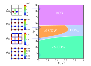
Figure 3: (Color online) SCMF phase diagram. Shown on the left are representatives of the on-site density $\rho_{ii}$, the nearest neighbor hopping $\rho_{ij}$ (with $j=i+\hat{x}$ or $j=i+\hat{y}$), or the pairing gap $\Delta_{ij}$ corresponding to the four phases at $V_{\text{d}}=0.5t$. Lattice size is $32\times 32$.

We now provide some intuitive understanding of the bond order phases by considering a simplified mean field version of Eq. (1), keeping only the nearest neighbor interactions $V_{x}$ and $V_{y}$. The mean field decoupling of the interaction term gives $-n_{i}n_{j}\sim a_{i}^{\dagger}a_{j}a_{j}^{\dagger}a_{i}\rightarrow\rho_{ij}a_{j}^{\dagger}a_{i}+h.c.-|\rho_{ij}|^{2}$. The modulation of the bond variable, $\rho_{ij}=\langle a^{\dagger}_{i}a_{j}\rangle$, in the BOS_p phase at $\phi_{\text{F}}=0$ has the form show in Fig. 1(c), $\rho_{i,i\pm\hat{x}}=\chi_{x}$, $\rho_{i,i\pm\hat{y}}=\chi_{y}\pm\delta$. The mean field Hamiltonian can be written as $H_{R}=-2\sum_{\mathbf{k}}\chi_{\mathbf{k}}b_{\mathbf{k}}^{\dagger}a_{\mathbf{k}}+h.c.$, up to a constant term. Here $a_{\mathbf{k}}$ and $b_{\mathbf{k}}$ are fermion annihilation operators defined separately on two sub-lattices related by the lattice translation vector $a_{\text{L}}\hat{x}$, and $\chi_{\mathbf{k}}=(t+V_{x}\chi_{x})\cos k_{x}+(t+V_{y}\chi_{y})\cos k_{y}-iV_{y}\delta\sin k_{y}$. The ground state energy per unit cell is then given by $E_{\text{GS}}=-2(\chi_{x}+\chi_{y})(t+V_{x}+V_{y})-2V_{y}\delta^{2}$, clearly indicating that finite bond modulation $\delta$ is energetically favored for positive $V_{y}$. The $\phi_{\text{F}}=90^{\circ}$ situation is identical, only with $x$ and $y$ axis interchanged, and hence a 90^∘ rotated bond pattern. Thus, the BOS_d phase, with checkerboard pattern of next-to-nearest bonds near $\phi_{\text{F}}=45^{\circ}$, naturally connects the two BOS_p phases on either side.

The bond modulation $\delta$, the energy gap, and the transition temperature $T_{c}$ of the BOS_p phase increase with $V_{\text{d}}$ for weak coupling. Exact diagonalization of Eq. (1) on a $2\times 8$ and $4\times 4$ cluster with periodic boundary conditions shows that the optimal place to observe the BOS_p is at intermediate interaction and tilt angle, e.g. $V_{\text{d}}\sim 2.5t$ and $(\theta_{\text{F}},\phi_{\text{F}})=(45^{\circ},0^{\circ})$, where the energy gap, and thus $T_{c}$, is maximal. Mean field theory estimates an optimal $T_{c}\sim 0.23t$, or about $0.05E_{F}$ for half filling, which is not too far from the temperature achieved in Dy experiment, $T\sim 0.25E_{F}$ priv . The BOS_d on the other hand is most stable in the vicinity of $\phi_{\text{F}}=45^{\circ}$ for $\theta_{\text{F}}\sim 60^{\circ}$. The characteristic density modulation of the $cb$-CDW and $st$-CDW phase uniquely distinguishes them from the other phases and may be detected via in-situ density imaging. The BCS phase can be detected via pair correlation measurements using noise spectroscopy lukin . Finally the BOS_d phase may be distinguished from BOS_p by probing the $d$-wave symmetry via the pump-probe scheme discussed in Ref. demler . Finally, in the presence of a trap potential, the insulating plateau at half filling will be surrounded by metallic regions. The approaches outlined here can be employed to study dipolar Fermi gas away from half-filling.

SB and EZ are supported by NIST Grant No. 70NANB7H6138 Am 001 and ONR Grant No. N00014- 09-1-1025A. LM acknowledges support from the Landesexzellenzinitiative Hamburg, which is financed by the Science and Research Foundation Hamburg and supported by the Joachim Herz Stiftung. SWT acknowledges support from NSF under grant DMR-0847801 and from the UC-Lab FRP under award number 09-LR-05-118602.

References

- (1) A. Griesmaieret al., Phys. Rev. Lett. 94, 160401 (2005).
- (2) M. Lu, N. Q. Burdick, S. H. Youn, and B. L. Lev, Phys. Rev. Lett. 107, 190401 (2011).
- (3) A. Micheli, G. K. Brennen, and P. Zoller, Nature Physics 2, 341 (2006).
- (4) A. V. Gorshkov et al., Phys. Rev. Lett. 107, 115301 (2011).
- (5) M. Lu, N. Q. Burdick, and B. L. Lev, arXiv:1202.4444.
- (6) K. -K. Ni et al., Science 322, 231 (2008).
- (7) A. Chotia et al., arXiv:1110.4420, (2011).
- (8) M. A. Baranov, Phys. Rep. 464, 71 (2008).
- (9) T. Lahaye et al., Rep. Prog. Phys. 72, 126401 (2009).
- (10) B. M. Fregoso, and E. Fradkin, Phys. Rev. Lett. 103, 205301 (2009).
- (11) C. -K. Chan, C. Wu, W. -C. Lee, and S. Das Sarma, Phys. Rev. A 81, 023602 (2010).
- (12) M. A. Baranov, L. Dobrek, and M. Lewenstein, Phys. Rev. Lett. 92, 250403 (2004).
- (13) M. A. Baranov, M. S. Mar’enko, V. S. Rychkov, and G. V. Shlyapnikov, Phys. Rev. A 66, 013606 (2002).
- (14) G. M. Bruun, and E. Taylor, Phys. Rev. Lett. 101, 245301 (2008).
- (15) N. R. Cooper, and G. V. Shlyapnikov, Phys. Rev. Lett. 103, 155302 (2009).
- (16) C. Zhao et al., Phys. Rev. A 81, 063642 (2010).
- (17) Y. Yamaguchi, T. Sogo, T. Ito, and T. Miyakawa, Phys. Rev. A 82, 013643 (2010).
- (18) K. Mikelsons, and J. K. Freericks, Phys. Rev. A 83, 043609 (2011).
- (19) J. Quintanilla, S. T. Carr, and J. J. Betouras, Phys. Rev. A 79, 031601(R) (2009).
- (20) K. Sun, C. Wu, and S. Das Sarma, Phys. Rev. B 82 075105 (2010).
- (21) C. Lin, E. Zhao, and W. V. Liu, Phys. Rev. B 81, 045115 (2010); Phys. Rev. B 83, 119901(E) (2011).
- (22) L. He and W. Hofstetter, Phys. Rev. A 83, 053629 (2011).
- (23) R. Shankar, Rev. Mod. Phys. 66, 129 (1994).
- (24) D. Zanchi and H. J. Schulz, Phys. Rev. B 61,13609 (2000).
- (25) L. Mathey, S. -W. Tsai, and A. H. Castro Neto, Phys. Rev. Lett. 97, 030601 (2006); Phys. Rev. B 75, 174516 (2007).
- (26) J.-P. Blaizot and G. Ripka, Quantum Theory of Finite Systems, MIT Press, Cambridge MA (1985).
- (27) M. Nakamura, Phys. Rev. B 61, 16377 (2000).
- (28) P. Sengupta, A. W. Sandvik, and D. K. Campbell, Phys. Rev. B 65, 155113 (2002).
- (29) K. -M. Tam, S. -W. Tsai, and D. K. Campbell, Phys. Rev. Lett. 96, 036408 (2006).
- (30) C. Nayak, Phys. Rev. B 62, 4880 (2000).
- (31) E. Altman, E. Demler, and M. D. Lukin, Phys. Rev. A 70, 013603 (2004).
- (32) D. Pekker, R. Sensarma, and E. Demler, arXiv:0906.0931.