Dekan:	Prof. Dr. Matthias Löwe
Erster Gutachter:	Prof. Dr. Raimar Wulkenhaar
Zweiter Gutachter:	Prof. Dr. Denjoe O’Connor
Tag der mündlichen Prüfung:
Tag der Promotion:

Zusammenfassung

Gegenstand der Arbeit ist die numerische Untersuchung einer über das Spektralwirkungsprinzip definierten nichtkommutativen Feldtheorie.
Ausgangspunkt dieser Konstruktion ist ein (als harmonisch bezeichnetes) spektrales Tripel $(\mathcal{A}_{4},\mathcal{H}_{4},\mathcal{D}_{4})$. Dabei ist $\mathcal{A}_{4}$ die 4-dimensionale nichtkommutative Moyal-Algebra und $\mathcal{D}_{4}$ ein selbstadjungierter (Dirac-)Operator auf dem Hilbert-Raum $\mathcal{H}_{4}$, so dass $\mathcal{D}_{4}^{2}$ der Schrödinger-Operator des 4-dimensionalen harmonischen Oszillators wird. Die Konstruktion dieser Daten basiert auf einer 8-dimensionalen Clifford-Algebra. Für das Produkt aus dem Tripel $(\mathcal{A}_{4},\mathcal{H}_{4},\mathcal{D}_{4})$ mit einem matrixwertigen spektralen Tripel wird analog zum Standardverfahren der nichtkommutativen Geometrie die Spektralwirkung
berechnet.

Die Renormierungstheorie assoziiert zur Spektralwirkung ein (z.T. nur formales) Wahrscheinlichkeitsmaß, deren zugehörige Korrelationsfunktionen eine Feldtheorie definieren. In der störungstheoretischen Variante wird das
Wahrscheinlichkeitsmaß als formale Potenzreihe konstruiert. Voraussetzung dafür ist die explizite Kenntnis der Lösungen der Euler-Lagrange-Gleichungen zur Spektralwirkung. Für das betrachtete Modell erweist es sich als unmöglich, diese Lösungen (als Vakuum bezeichnet) zu gewinnen.

Ein alternatives Verfahren besteht in der Diskretisierung aller Variablen und der numerischen Untersuchung des Verhaltens der Korrelationsfunktionen bei Verfeinerung der Diskretisierung. Die Diskretisierung des Modells wird durch die Matrix-Basis des Moyal-Raums und Beschränkung auf endliche Matrizen erreicht. Durch Monte-Carlo-Simulationen werden wichtige Korrelationsfunktionen wie die Energiedichte, die spezifische Wärme sowie einige Ordnungsparameter untersucht, sowohl in Abhängigkeit von der Größe der Matrizen als auch von den unabhängigen Parametern des Modells. Dabei werden trotz der großen Komplexität der approximierten Spektralwirkung verläßliche numerische Resultate erzielt, die zeigen, daß eine numerische Behandlung dieser Art von Modellen in der Matrix-Moyal-Basis möglich ist.

Abstract

The object of this work is the numerical investigation of a non-commutative field theory defined via the spectral action principle. Starting point of this construction is a spectral triple $(\mathcal{A}_{4},\mathcal{H}_{4},\mathcal{D}_{4})$ referred to as harmonic. Here, $\mathcal{A}_{4}$ is the 4-dimensional (noncommutative) Moyal algebra, and $\mathcal{D}_{4}$ is a selfadjoint (Dirac-)operator on the Hilbert space $\mathcal{H}_{4}$ such that $\mathcal{D}_{4}^{2}$ is the Schrödinger operator of the 4-dimensional harmonic oscillator. The construction of these data relies on an 8-dimensional Clifford algebra. In analogy to the standard procedure of non-commutative geometry, the spectral action is computed for the product of the triple $(\mathcal{A}_{4},\mathcal{H}_{4},\mathcal{D}_{4})$ with a matrix-valued spectral triple.

Renormalization theory associates to the spectral action a (often only formal) probability measure. Its associated correlation functions define then a field theory. In the perturbative approach this measure is constructed as a formal power series. This requires explicit knowledge of the solutions of the Euler-Lagrange equations for the spectral action. For the model under consideration, it turns out impossible to obtain these solutions.

An alternative approach consists in a discretization of all variables and a numerical investigation of the behavior of the correlation functions when the discretization becomes finer. For the model under consideration, the discretization is achieved in the matrix basis of the Moyal algebra restricted to finite matrices. By Monte Carlo simulation we study several important correlation functions such as the energy density, the specific heat and some order parameters, in dependence both of the matrix size and of the independent parameters of the model. Despite the complexity of the approximated spectral action, some reliable numerical results are obtained, showing that a numerical treatment of this kind of models in the Moyal matrix basis is possible.

Introduction

The main object of this work is a particular non-commutative field theory which is derived using the spectral action principle and then treated numerically. Non-commutativity can be found in many fields of physics like quantum field theories, string theory [5], condensed matter physics. The first application of non-commutativity into physicss is dated from the middle of the last century inspired by the ideas of quantum mechanics, where starting from classical mechanics, the commutative algebra of functions on the phase space is replaced by a non-commutative operator algebra on a Hilbert space. The duality between ordinary spaces $M$ and proper commutative algebras is expressed by the Gel’fand-Naimark theorem which states the fact that the algebra of all continuous functions on $M$ is the only possible type of commutative $C^{*}$-algebra. Additionally, given a commutative $C^{*}$-algebra $C$, it is possible to reconstruct a Hausdorff topological space $M$ in order to obtain that $C$ is the algebra of continuous functions on $M$. The study of commutative $C^{*}$-algebras is equivalent to the study of topological Hausdorff spaces. The previous duality has inspired the identification, in non-commutative geometry, of some algebraical objects as a category of non-commutative topological spaces. Alain Connes [31], one of the founders of non-commutative geometry, has proposed a candidate for the objects of such category, the spectral triples $(\mathcal{A},\mathcal{H},\mathcal{D})$ [32], composed by an algebra $\mathcal{A}$, an Hilbert space $\mathcal{H}$ on which $\mathcal{A}$ is represented and an selfadjoint operator $\mathcal{D}$. In fact, every compact oriented Riemannian manifold can be used to define a spectral triple, this kind of manifold $M$ characterizes a symmetric Dirac type operators on self-adjoint Clifford module bundles over $M$. Connes, after a conjecture in 1996 [36] and some considerable attempts of Rennie and Varilly [67], proved the so called reconstruction theorem [33] for commutative spectral triples satisfying various axioms, showing that exists a compact oriented smooth manifold $X$ such that $A=C^{\infty}(X)$ is the algebra of smooth functions on $X$ and every compact oriented smooth manifold emerges in this way. Pushed by the aim of reformulating the standard model of particles in a non-commutative way [35, 36], Connes has introduced the almost-commutative spectral triple extending the axioms of the reconstruction theorem to a non-commutative algebra. The almost-commutative spectral triples are defined as the non-commutative Cartesian product of a commutative spectral triple of a compact spin manifold, with a spectral triple where the Hilbert space is finite-dimensional, this triples are often labeled as finite spectral triple.

A field theory can be interpreted [3] as a theory concerning maps $\phi$ (usually referred as fields) between the space-time $M^{\prime}$ and a target space $M$. On this spaces are defined some structures, they can be Riemannian or pseudo-Riemannian manifold depending on the signature of the space-time. A fundamental role in the field theory is played by the action $S(\phi)$ which is a functional of the elementary fields in the theory. In the classical theory the aim is to study the extrema of the action functional $\delta S(\phi_{0})=0$ in order to obtain the solution of the equations of motion. Quoting the intuitive Feynman formulation of quantum field theory [61], the action is used to study the functional integrals:

$$\int_{\phi}D\phi F(\phi)e^{-\frac{1}{\hslash}S(\phi)}$$

where $F(\phi)$ is a functional of $\phi$ and $D\phi$ is the functional measure. The previous expression in general is not well defined and should be considered as an approximate expression. However, the functional integral approach is very useful in studying the quantum field theory connection with the expectation values in statistical mechanics; all field configurations contributes in the estimation of the previous functional each whit probability amplitude $P(\phi)\sim e^{-\frac{1}{\hslash}S(\phi)}$. More formally the action functional is used to compute the correlation functions which are one the main physical output of a quantum field theory with a close connection to the experimental measurements. In the path integral formalism [62] the correlation function of the fields $\phi_{1}(x_{1})\cdots\phi_{n}(x_{n})$ is given, for the euclidean case, by the functional integral:

$$\int D\Phi\phi_{1}(x_{1})\cdots\phi_{n}(x_{n})e^{-S(\phi_{i})}$$

where is the path integral measure $D\Phi$ on the space of configuration of the elementary fields. In the Lorentz signature the last term is replaced by $e^{iS}$. A crucial point in the quantum field theory is the formalization of the previous integral in order to obtain all correlation functions of the theory well defined. This procedure is called renormalization and is achieved using a perturbative approach. A safe perturbative analysis can only be conducted after expanding the action around its vacuum, of course this requirement needs the explicit expression for the vacuum usually obtained minimizing the action. It is clear that for any quantum field theory the explicit determination of vacuum is a indispensable step before the perturbative study of its renormalizability can be done.

In order to define an action for a non-commutative geometry theory Connes and Chamsedinne introduced a general formalism for spectral triples, the spectral action principle [53]. The term spectral come from the fact that it depends only on the spectrum of the Dirac operator and it takes the form

$$\textrm{Tr}(\chi(\mathcal{D}/\Lambda))$$

where $\Lambda$ is a real parameter and it fixes the energy scale. The $\chi$ is a differentiable function $\chi:\mathbb{R}_{+}\to\mathbb{R}_{+}$ of sufficiently fast decrease such that the spectral action converges.

Using this approach the standard model of particles has been reformulated, including a Riemannian formulation of gravity. The algebra of the spectral triple used is defined by the tensor product of $C^{\infty}(M)$, the regular functions on a manifold $M$, times a matrix algebra of finite dimension. Formally the natural group of invariance of the standard model, including gravity, is the semidirect product:

$$G=\mathcal{U}\rtimes\textrm{Diff}(M)$$

Were $\mathcal{U}=C^{\infty}(M,U(1)\times SU(2)\times SU(3))$ is the group of local gauge transformations. The total group of invariance admits $\mathcal{U}$ as a normal subgroup. A.Connes has showed, defining $\mathcal{A}=C^{\infty}(M)\otimes(C\oplus\mathbb{H}\oplus M_{3}(C))$, that the automorphisms group Aut($\mathcal{A}$) of the non-commutative algebra $\mathcal{A}$ admits the inner group Int($\mathcal{A}$) as a normal subgroup and Aut$(A)\approx G$. The algebra $\mathcal{A}_{F}=(C\oplus\mathbb{H}\oplus M_{3}(C))$ is finite and $\mathbb{H}$ is the algebra of quaternions. The rest of the spectral geometry is defined by the action of $\mathcal{A}$ on $\mathcal{H}$ and by suitable Dirac operator operator $\mathcal{D}$. In [53] is showed that the total spectral triple is given by:

$$(\mathcal{A},\mathcal{H},\mathcal{D})=(C^{\infty}(M),L^{2}(M,S),\ \not{\partial}_{M})\otimes(\mathcal{A}_{F},\mathcal{H}_{F},\mathcal{D}_{F})$$

with

$$\mathcal{H}=L^{2}(M,\mathcal{S})\otimes\mathcal{H}_{F},\ \mathcal{D}=\not{\partial}_{M}\otimes 1+\gamma_{5}\otimes\mathcal{D}_{F}$$

The algebra $\mathcal{A}_{F}$ is finite dimensional so the dimension of the corresponding Hilbert space $\mathcal{H}_{F}$ must be finite dimensional [51]. The final step, in order to obtain a field theory, is to define an action, this task is achieved using the spectral action principle and the invariance under the symmetry group is implement fluctuating the Dirac operator. The subgroup Int$(\mathcal{A})$ of inner automorphisms is a normal subgroup and the group Aut$(\mathcal{A})$ of diffeomorphisms falls in equivalence classes under Int$(\mathcal{A})$. This induces a natural foliation into equivalence classes in the space of metrics. The internal fluctuations [38] of a given metric are given by the formula:

$$\mathcal{D}=\mathcal{D}_{0}+A+JAJ^{-1},\ \ A=\sum a_{i}[D_{0},b_{i}]\ a_{i},b_{i}\in\mathcal{A}$$

where $J$ is the real structure. In this way starting from $(\mathcal{A},\mathcal{H},\mathcal{D}_{0})$, instead modify the representation of $\mathcal{A}$ in $\mathcal{H}$, it is changed the operator $\mathcal{D}_{0}$ where $A$ is a self-adjoint operator in $\mathcal{H}$ of the form $A=\sum a_{i}[\mathcal{D}_{0},b_{i}]$. The spectral action principle applied to inner fluctuations reproduces the bosonic part of the model, the gravity is naturally present in the model, while the other interactions are encoded in the matrix algebra of the total spectral triple. The non-commutativity of matrices corresponds to the non-abelianity of the gauge theory defining a so called Yang-Mills theory.

The previous example of application of non-commutative geometry to a field theory is founded on the use of a spectral triple where the algebra is almost-commutative, a very interesting task is to formulate a field theory for a truly non-commutative algebra. A first attempt was obtained replacing in the usual field theory action the point-wise multiplication of the fields with a non-commutative one, namely a $\star$-product. The fields now belongs to $\mathbb{R}^{4}_{\Theta}$, a vector space defined by an enough regular class functions on $\mathbb{R}^{4}_{\Theta}$ equipped with the Moyal product:

$$(f\star g)(x)=\int\int d^{4}y\frac{d^{4}k}{(2\pi)^{4}}f(x+\frac{1}{2}\Theta\cdot k)g(x+y)e^{i\langle k,y\rangle}$$

Where $\Theta$ is a skew-symmetric matrix. Unfortunately all the attempts to renormalize such quantum field theories on the non-commutative $\mathbb{R}^{4}$ failed and these models show a phenomenon called UV/IR-mixing [13, 14, 15]. A great step towards the non-commutative field theory was made when H.Grosse and R.Wulkenhaar [44], found a non-commutative $\varphi^{4}$-theory renormalizable action which develops additional marginal coupling, corresponding to an harmonic oscillator potential for the real-valued free field $\varphi$ on $\mathbb{R}^{4}_{\Theta}$ :

$$S[\varphi]=\int d^{4}x\left(\frac{1}{2}\varphi\star(-\Delta+\Omega^{2}\tilde{x}^{2}+\mu^{2})\star\varphi+\frac{\lambda}{4}\varphi\star\varphi\star\varphi\star\varphi\right)(x)$$

Where $x=2\Theta^{-1}\cdot x,\ \lambda\in\mathbb{R}\ \Omega\in[0,1]$, and $\mu$ is a real parameter. Using the Moyal matrix base, which turns the $\star$-product into a standard (infinite) matrix product, H.Grosse and R.Wulkenhaar were able to prove the perturbative renormalizability of the theory [43]. Afterward, R.Wulkenhaar et al. [18] found an alternative simpler normalization proof using multi-scale analysis in matrix base, showing the equivalence of various renormalization schemes. A last, but useful, renormalization proof was formulated using Symanzik type hyperbolic polynomials [21]. It is worthwhile to mention [21, 22].

The non-commutative model treated in this thesis is a sort of extension, via spectral action principle, of the scalar W-G model, in which we are interested to formulate a Yang-Mills theory in renormalizable way on Moyal space. From the previous discussions we can expect that usual Yang-Mills theory on Moyal space without modifications of the action by something similar to an oscillator potential, to be not renormalizable [16]. Additionally, the Moyal space with usual Dirac operator is a spectral triple, the corresponding spectral action was computed in [53], with the result that it is the usual not renormalizable action on Moyal plane. In [45] H.Grosse and R.Wulkenhaar, in order to obtain a gauge theory with an oscillator potential via the spectral action principle, used a Dirac operator constructed using the statement $\mathcal{D}^{2}=H$ where the four dimensional Laplacian is substituted by the four dimensional oscillator Hamiltonian $H=-\Delta+\Omega^{2}||x||^{2}$. The idea behind is that the spectral dimension is defined through the Dirac operator so the spectral dimension defined by such Dirac operator is related to the harmonic oscillator phase space dimension. It turns out that to write down an Dirac operator, so that its square equals the 4D harmonic oscillator Hamiltonian, is an easy task using eight dimension Clifford algebra. In addition, can be shown that using this Dirac operator on 4D-Moyal space, is possible define an eight-dimensional spectral triple. In this thesis is used the approach described in [57] in which the Dirac operator is constructed using $n$-dimensional bosonic and fermionic creation and annihilation operators. After defined the Dirac operator with the desired spectrum it is considered the total spectral triple as the tensor product of the ”oscillating” spectral triple $(\mathcal{A}_{4},\mathcal{H}_{4},\mathcal{D}_{4})$ with an almost-commutative triple and then is perform the previous described procedure of non-commutative geometry to compute the spectral action. We notice that matrix algebra introduces an extension of the standard potential in the commutative case, in fact the scalar field $\phi$ and the $X_{\mu}$ fields are present together in a potential of the form $(\alpha X_{\mu}\star X^{\mu}+\beta\bar{\varphi}\star\varphi-1)^{2}$, with $\alpha,\beta\in\mathbb{R}^{+}$ and $X_{\mu}(x)=(\Theta^{-1})_{\mu}^{\nu}x_{\nu}+A_{\mu}(x)$ is a covariant coordinate. These two additional terms, the integral over $X_{\mu}\star X^{\mu}$ and over its square, were conjectured in [46].

The high non-triviality of the vacuum makes very difficult to explicit the vacuum configuration of the system in [71] A. de Goursac, J.C. Wallet, and R. Wulkenhaar, using the matrix base formalism, have found an expressions from vacuum solutions deriving them from the relevant solutions of the equations of motion. Although, the complexity of the vacuum configuration makes the perturbative approach very complicated, in order to conduct some investigations in this thesis will be considered a non-perturbative scheme using a discretized matrix model of the action in which the fields become matrices, the star product become the matrix multiplication and the integral turns in a matrix trace.

Now comes in to play the numerical treatment, the standard method is to approximate the space by discrete points, for example using a lattice approximation and then calculate the observables over that set of points [76]. Since an approximation in the position space is not suitable due to the oscillator factor of the Moyal product, instead the lattice approximation, will be used the matrix Moyal base, which was already used in the first renormalization proof of $\varphi^{4}$-model restricted to finite matrices. Hence, will be performed a Monte Carlo simulation studying some statistical quantity such the energy density and specific heat varying the parameters $\Omega,\frac{\chi_{-1}}{\chi_{0}},\alpha$ and gathering some informations on the various contributions of the fields to the action. The simulations are quite cumbersome due the complexity of the action and the number of independent matrices to handle but using particular algorithm we are able to get an acceptable balance between the computation precision and the computation time. For the simulations is applied a standard Metropolis-Monte Carlo algorithm [75] with various estimators for the error (see appendix B) and for the autocorrelation time of the samples. The initial conditions of the Markov chain are chosen randomly in the phase space, they can be of two types; hot initial conditions, which are configurations far from the minimum, and cold start conditions, which correspond to configurations close to the minimum of the action. In general we chose the range of parameters in order to avoid problems with the thermalization process, obtaining numerical simulations where is enough to wait a relative small number of Monte Carlo steps to compute independent results from the initial conditions. For the model under study, we are interested on the continuous limit that correspond to matrices of infinite size. We will consider various size of the matrices expecting a stabilization of the values of observables like the energy density, increasing the matrix size. In order to find same possible phase transitions will be used the specific heat which is a measure of the dispersion of the energy. The phase transitions are registered as peaks of the specific heat, increasing the matrices size. Beside, we define others quantities, such as $\langle\textrm{Tr}[\varphi]^{2}\rangle$ and $\langle\sum_{n=0}^{N}|\varphi_{nn}|^{2}\rangle$ which are used as order parameters [81], we have also defined their susceptibilities but are not collected due the high number of samples required to obtain a sufficient precision

Plan of the work

This work is structured in order to introduce the reader to the model treated and to the numerical analysis, using an heuristic approach. The first chapter and the third one are introductory chapters in which are explained respectively the fundamentals non-commutative geometry and the main concepts of Monte Carlo numerical simulation. In particular in the first chapter we will introduce the mathematical tools and the machinery required to formulate our spectral model. In the first part of chapter one will be described the basics of non-commutative geometry, Weyl-Wigner map. Further will be introduced some notions of spectral geometry and in the end will presented a simple example of application of the spectral action principle. The second chapter is devoted to construct the W-G spectral action model. Will be described how to construct the harmonic Dirac operator starting from the one-dimensional case and then generalizing it using annihilations and creations operators for the bosonic and fermionic sectors. Having the 4D-Dirac harmonic operator with harmonic oscillator spectrum and extending it to an spectral triple, will be considered the tensor product of the non-commutative triple with a finite Connes-Lott type spectral triple [37]. Following the previous described standard procedure of non-commutative geometry, to obtain a ”gauged” Dirac operator, we will fluctuate the total Dirac operator, thus we will proceed to compute the spectral action in which are present two U(1)-Moyal Yang-Mills fields unified with a complex Higgs field. In the end of the chapter will be discussed some aspects of the resulting action in particular of vacuum and the needs for numerical treatment. The third chapter is an introduction to Monte Carlo analysis, will be set up all the ingredients required to conduct a numerical simulation of the model treated in the previous chapter. Will be explained the basics of the Monte Carlo simulation, focusing ourself on the application in the field theory. In the first sections of chapter three will be briefly discussed the path integral formulation, this formulation is essential to connect the field theories to statistical systems in which the Monte Carlo methods are born. Then will be introduced the Metropolis algorithm used to produce a Markov chain. In order to resume all the previous concepts and to show an example of phase analysis will be presented an application of numerical simulation on the well know Ising model. Right before the presentation of the numerical results, in the chapter 4, will be showed how the Monte Carlo it is implemented in our case starting from the discretization scheme introducing the Moyal base. In the second part, in order to define the observables of the upcoming Monte Carlo simulation, will be designated the expectation values, statistical quantities like energy, specific heat and the order parameters. Finally, in the last chapter will be showed the numerical results for the previous defined quantities for the full 4-dimensional model and for the 2-dimensional one.

Chapter 1 Introduction to Connes-Lott models

In this chapter we introduce some mathematical tools taken from non-commutative geometry in order to define a spectral triple, a spectral action and Connes-Lott models. In the first part of this chapter we describe the fundamentals of non-commutative geometry in particular the Weyl-Wigner map, further will be introduced some notions of spectral geometry.

1.1 Non-commutative geometry and
Weyl-Wigner map

In this section we will discuss, as an example of non-commutative space, the fate of the classical phase space under the process of quantization. This is a very large topic and we limit ourselves to some aspects. In particular we wish to introduce a way to quantize the phase space (and in general an $L^{2}(\mathbb{R}^{n})$ space) in which the quantized space can be seen as either a set of operators on an Hilbert space or as a deformation of the product of functions on the classical space. At least in the simple cases, the non-commutative algebra of a quantum phase space can be taken as the one generated by the position and momentum operators acting on a separable Hilbert space. We now establish a connection between the classical and quantum phase spaces, at least for systems with a well defined classical counterpart. We want to associate to each classical observable an bounded operator on $\mathcal{H}$. This will be done by the Weyl map [1]. Starting from the correspondence principle, an immediate problem is to solve an ordering ambiguity, beside $p$ and $q$ are unbounded operators, additionally arises problems about the definition of their domains. To solve these problems Weyl has suggested to introduce a base in the operator space on $L^{2}(\mathbb{R})$ using the unitary operators:

$$U(q)=e^{\frac{i}{\hslash}qP}$$ (1.1)

$$V(p)=e^{\frac{i}{\hslash}pQ}$$ (1.2)

Where $P$ and $Q$ are respectively the momentum operator and the position one. Being bounded, their domains can be extended to the whole Hilbert space $L^{2}(\mathbb{R})$. In general it is convenient to use the base defined by the following unitary operators:

$$W(\alpha,\beta)=e^{\frac{i}{\hslash}(\alpha P+\beta{Q})}$$ (1.3)

Where $\alpha$ and $\beta$ are two real parameters. A generic operator using this base can be expanded like:

$$F(P,Q)=\frac{1}{2\pi\hslash}\int_{\mathbb{R}^{2}}g(\alpha,\beta)e^{\frac{i}{\hslash}(\alpha P+\beta{Q})}d\alpha d\beta$$ (1.4)

Beside this expansion let us considering the base of $L^{2}(\mathbb{R}^{2})$:

$$w(\alpha,\beta)=e^{\frac{i}{\hslash}(\alpha p+\beta q)}$$ (1.5)

using this base any function can be written as

$$f(p,q)=\frac{1}{2\pi\hslash}\int_{\mathbb{R}^{2}}\tilde{f}(\alpha,\beta)e^{\frac{i}{\hslash}(\alpha p+\beta q)}d\alpha d\beta$$ (1.6)

where $\tilde{f}(\alpha,\beta)$ is the Fourier transform of $f(p,q)$. Now, thanks to the expansion (1.6) and (1.4), it is possible to build an application which maps each function in $L^{2}(\mathbb{R}^{2})$ to an bounded operator. In order to construct this map we use the function $\tilde{f}(\alpha,\beta)$ in the operatorial expansion (1.4). In such a way the ordering problem is solved, in fact the association is no more ambiguous.

Formally the Weyl map is the application:

$$\Omega:L^{2}(\mathbb{R}^{2})\to\mathcal{B}(\mathcal{H})$$

defined by

$$f(p,q)\rightarrow\Omega(f)(P,Q)=\frac{1}{2\pi\hslash}\int_{\mathbb{R}^{2}}\tilde{f}(\alpha,\beta)W(\alpha,\beta)\mbox{d}\alpha\mbox{d}\beta$$ (1.7)

with

$$\tilde{f}(\alpha,\beta)=\frac{1}{2\pi\hslash}\int_{\mathbb{R}^{2}}f(p,q)e^{-\frac{i}{\hslash}(\alpha p+\beta q)}\mbox{d}p\mbox{d}q$$ (1.8)

This particular Weyl map selects a certain ordering: the symmetric ordering or the so called Weyl’s ordering. Other ordering are possible, for example normal ordering or Wick ordering, introducing into (1.7) a weight function [6]. In addition, Weyl map is linear and satisfies the condition:

$$\Omega(\overline{f})=\Omega(f)^{\dagger}$$ (1.9)

In particular, if $f$ is real, then

$$\Omega(f)=\Omega(f)^{\dagger}$$ (1.10)

in other words $\Omega(f)$ is symmetric. The inverse of Weyl map, the so called Wigner map [2], is the map which associates to each operator a function of $p$ and $q$, it is defined by

$$\Omega^{-1}(F)(p,q)\equiv\frac{1}{(2\pi\hslash)^{2}}\int_{\mathbb{R}^{2}}e^{-\frac{i}{\hslash}(\alpha p+\beta q)}\operatorname{Tr}(FW^{\dagger}(\alpha,\beta))\mbox{d}\alpha\mbox{d}\beta$$ (1.11)

with $F\in\mathcal{B}(\mathcal{H})$. In fact, combining (1.7) and (1.11) we obtain:

$$\Omega^{-1}(\Omega(f))(p,q) = \frac{1}{(2\pi\hslash)^{2}}\int_{\mathbb{R}^{2}}\mbox{d}\alpha\mbox{d}\beta e^{-\frac{i}{\hslash}(\alpha p+\beta q)}\operatorname{Tr}\left(\Omega(f)W^{\dagger}(\alpha,\beta)\right)$$ (1.12)

$$\operatorname{Tr}\left(\Omega(f)W(\alpha,\beta)\right) = \operatorname{Tr}\left(\int_{\mathbb{R}^{2}}\frac{1}{2\pi\hslash}\tilde{f}(\xi,\eta)W(\xi,\eta)\mbox{d}\xi\mbox{d}\eta W^{\dagger}(\alpha,\beta)\right)$$ (1.13)

The integral of the previous relation is in d$\xi$ d$\eta$, assuming that the trace and the $W^{\dagger}(\alpha,\beta)$ can be switched with the integral and using the identity :

$$\operatorname{Tr}e^{\frac{i}{\hslash}(\alpha P+\beta{Q})}=\int_{\mathbb{R}^{2}}e^{\frac{i}{\hslash}(\alpha p+\beta{q})}\mbox{d}p\mbox{d}q=(2\pi\hslash)^{2}\delta(\alpha,\beta)$$ (1.14)

we obtain

$$\operatorname{Tr}\left(\Omega(f)W(\alpha,\beta)\right)=2\pi\hslash\int_{\mathbb{R}^{2}}\tilde{f}(\xi,\eta)\delta(\xi-\alpha,\eta-\beta)\mbox{d}\xi\mbox{d}\eta$$ (1.15)

Therefore (1.12) becomes:

$$\Omega^{-1}(\Omega(f))(p,q)=\frac{1}{2\pi\hslash}\int_{\mathbb{R}^{2}}\tilde{f}(\alpha,\beta)e^{\frac{i}{\hslash}(\alpha p+\beta q)}\mbox{d}\alpha\mbox{d}\beta$$ (1.16)

The left side is exactly the inverse Fourier transform of $f(\alpha,\beta)$. Finally we obtain:

$$\Omega^{-1}(\Omega(f))(p,q)=f(p,q)$$ (1.17)

this shows that the Wigner map is actually the inverse application Weyl map (1.11).

For simplicity, this construction used functions defined on $\mathbb{R}^{2}$ but can be extended to $\mathbb{R}^{n}$ without difficulties. In general using an $n$-dimensional base is possible to define a one to one correspondence between a function of $\vec{p}$ and $\vec{q}$ with an operator using their expansion in each space [25, 27].

1.2 Moyal product

Using Weyl map it is possible to define a new product in order to describe a quantum system, the Moyal product or star product. This new product is no longer commutative and is obtained combining Weyl map applied on two elements of the continuum space, with the Winger map applied on the product of the previous transformed elements.
Formally the Moyal product [26] is defined by

$$f\star g=\Omega^{-1}(\Omega(f)\Omega(g))$$ (1.18)

This star product is associative but non-commutative and satisfies the condition

$$(\alpha f)\star g=\alpha(f\star g)=f\star(\alpha g)$$ (1.19)

with $\alpha\in\mathbb{C}$. In addition, it satisfies the condition

$$\overline{f\star g}=\overline{g}\star\overline{f},$$ (1.20)

the Leibniz rule

$$\frac{\partial}{\partial x^{i}}(f\star g)=\frac{\partial f}{\partial x^{i}}\star g+f\star\frac{\partial g}{\partial x^{i}}$$ (1.21)

with $i\in\{1,2,\ldots,n\}$ and the condition

$$\int_{\mathbb{R}^{n}}f(x)\star g(x)\mbox{d}x=\int_{\mathbb{R}^{n}}f(x)g(x)\mbox{d}x$$ (1.22)

from which follows that the integral has trace property:

$$\int_{\mathbb{R}^{n}}f(x)\star g(x)\mbox{d}x=\int_{\mathbb{R}^{n}}g(x)\star f(x)\mbox{d}x$$ (1.23)

It is possible to show [29] that, for $f$ and $g$ analytic, the star product can be written as

$$(f\star g)(q,p)=f(q,p)e^{\frac{i\hslash}{2}\left(\frac{\stackrel{{\scriptstyle\leftarrow}}{{\partial}}}{\partial q^{i}}\frac{\stackrel{{\scriptstyle\rightarrow}}{{\partial}}}{\partial p_{i}}-\frac{\stackrel{{\scriptstyle\rightarrow}}{{\partial}}}{\partial q^{i}}\frac{\stackrel{{\scriptstyle\leftarrow}}{{\partial}}}{\partial p_{i}}\right)}g(q,p)$$ (1.24)

or equivalently

$$(f\star g)(q,p)=\sum_{n=0}^{\infty}f(q,p)\frac{1}{n!}\left[\frac{i\hslash}{2}\left(\frac{\stackrel{{\scriptstyle\leftarrow}}{{\partial}}}{\partial q^{i}}\frac{\stackrel{{\scriptstyle\rightarrow}}{{\partial}}}{\partial p_{i}}-\frac{\stackrel{{\scriptstyle\rightarrow}}{{\partial}}}{\partial q^{i}}\frac{\stackrel{{\scriptstyle\leftarrow}}{{\partial}}}{\partial p_{i}}\right)\right]^{n}g(q,p)$$ (1.25)

where the arrows point the direction in which the partial derivate acts.
The expression is well defined only on a quite small set of functions, however can be obtained some integral expressions with larger domains [29]:

$$(f\star g)(u):=\frac{1}{(\pi\hslash)^{-n}}\int_{\mathbb{R}^{n}}\int_{\mathbb{R}^{n}}f(v)g(w)e^{\frac{2i}{\hslash}(u-v)\cdot\Theta^{-1}\cdot(u-w)}\mbox{d}v\mbox{d}w$$ (1.26)

Equivalent formulas  are

$$(f\star g)(u):=\frac{1}{(\pi\hslash)^{-n}}\int_{\mathbb{R}^{n}}\int_{\mathbb{R}^{n}}f(u+v)g(u+w)e^{\frac{2i}{\hslash}v\cdot\Theta^{-1}\cdot w}\mbox{d}v\mbox{d}w$$ (1.27)

or

$$(f\star g)(u):=\frac{1}{(\pi\hslash)^{-n}}\int_{\mathbb{R}^{n}}\int_{\mathbb{R}^{n}}f(u+\frac{\hslash}{2}\Theta\cdot v)g(u+w)e^{iv\cdot w}\mbox{d}v\mbox{d}w$$ (1.28)

A very useful remark is that Moyal product becomes the usual one in the limit $\hslash\to 0$, in other words Moyal product can be viewed like a deformation usual product in the deformation parameter $\hslash$. Therefore, we can interpret the quantum mechanic phase space as a deformation of classical mechanic phase space obtained substituting the point wise product with Moyal one. This product will be used in the next chapter to construct a non-commutative $\mathbb{R}^{4}_{\Theta}$ vector space the so called Moyal plane.

It is possible to give some matrix basis for the algebra of functions on a two dimensional phase space with the star product. Defined the functions (taking $\hslash=1$)

$$\begin{array}[]{cc}a=\frac{1}{\sqrt{2}}(q+iq)&\bar{a}=\frac{1}{\sqrt{2}}(q-ip)\\ \end{array}$$ (1.29)

for a generic function results

$$\begin{array}[]{cc}a\star f=af+\frac{\partial f}{\partial\bar{a}}&f\star a=af-\frac{\partial f}{\partial\bar{a}}\\ \end{array}$$ (1.30)

and similar relations for $\bar{a}$. The function

$$\varphi_{0}=2e^{\frac{q^{2}+p^{2}}{2}}$$ (1.31)

is Gaussian and has the useful property that

$$\varphi_{0}\star\varphi_{0}=\varphi_{0}$$ (1.32)

Defining the functions

$$\varphi_{mn}=\frac{1}{\sqrt{2^{n+m}n!m!}}\bar{a}^{n}\star\varphi_{0}\star a^{m}$$ (1.33)

and using the relations (1.30) and (1.32) it is easy to show that

$$\varphi_{mn}\star\varphi_{kl}=\delta_{nk}\varphi_{ml}$$ (1.34)

Therefore the $\varphi$’s can be used as a base [29] for the deformed algebra and the star multiplication becomes the usual multiplication of (infinite) matrices.

1.3 Spectral geometry

In this section we introduce the argument of Connes’ spectral geometry which is the non-commutative generalization of a usual geometry on a manifold. In particular we will introduce some basic concepts like non-commutative infinitesimals and the Dixmier trace as algebraic generalization of the usual infinitesimals and of the integral [28, 31, 24]. A fundamental role will be taken by the generalized Dirac operator, with which we will define the metric of a non-commutative space and the spectral action of a Connes-Lott Model [50, 52].

1.3.1 Non-commutative infinitesimals

To define the Diximier trace we need some facts about compact operators [47]. Let us recall that an operator $A$ belonging $C^{*}$-algebras of bounded operators over an Hilbert space $\mathcal{H}$, namely $A\in\mathcal{B}(\mathcal{H})$, is called of finite rank if the orthogonal complement of its kernel is finite dimensional. Roughly speaking, even if the Hilbert space is infinite dimensional, such operators are finite dimensional matrices. Beside an operator $A$ on $\mathcal{H}$ is compact if it can be approximated in norm by finite rank operators. An equivalent way to characterize a compact operator $A$ is that $\forall\epsilon>0$ exists a subspace of finite dimension $E\subset\mathcal{H}$ which satisfies $\parallel A\mid_{E^{\perp}}\parallel<\epsilon$.
Taking in account the previous characterization of compact operators they can be seen in some sense small, so they are good candidates to be infinitesimals. Calling $\mathcal{K}(\mathcal{H})\subset\mathcal{B}(\mathcal{H})$ the subset of the compact operators, the size of the infinitesimal $A\in\mathcal{K}(\mathcal{H})$ can be defined by the rate of decay of a sequence $a_{n}(A)$ when $n\rightarrow\infty$. Where $\{a_{n}(A)\}$ are the non vanishing eigenvalues of the operator $|A|$ arranged with repeated multiplicity.
The infinitesimals of order $\alpha$ are all the operators $A\in\mathcal{K}(\mathcal{H})$ such that it is possible to to construct a sequence satisfying:

$$\begin{array}[]{l}a_{n}(A)=O(n^{-\alpha})\ \textrm{as}\ n\rightarrow\infty,\\ \\ \exists\ C<\infty\mid a_{n}(A)\leq Cn^{-\alpha},\forall n\geq 1.\end{array}$$ (1.35)

Remark:

The algebra $\mathcal{K}(\mathcal{H})$ is the only norm closed and two-sided ideal when $\mathcal{H}$ is separable and it is essential, therefore is the largest two-sided ideal in the $C^{*}$-algebra $\mathcal{B}(\mathcal{H})$. Since the identity operator I on an infinite dimensional Hilbert space is not compact the algebra is not unital. Beside the defining representation of $K(\mathcal{H})$ is the only, up to equivalence, irreducible representation of $K(\mathcal{H})$, in fact it is Morita equivalent to the algebras of finite rank matrices of complex numbers.

1.3.2 The Dixmier Trace

The Dixmier trace is a trace on a space of linear operators on an Hilbert space larger than the space of trace class operators. This trace is defined in order to have the infinitesimals of order $1$ in its domain but the higher order infinitesimals have vanishing trace. With this requirements the standard trace, with domain in the two-sided ideal $\mathcal{L}^{1}$ of trace class operators, is not suitable. The usual trace, defined as $\operatorname{Tr}A:=\sum_{n}\left\langle A\xi_{n},\xi_{n}\right\rangle$, for any $A\in\mathcal{L}^{1}$, is independent of the orthonormal basis $\xi_{n},\ n\in N$ of $\mathcal{H}$. In the case of a positive and compact operator $A$, the eigenvalues becomes positive and the definition turn to be $\operatorname{Tr}A:=\sum_{n=0}^{\infty}a_{n}(A)$. In general, an infinitesimal of order $1$ is not in $\mathcal{L}^{1}$, since we can not ensure the convergence of its characteristic values, we can just say that $a_{n}(A)\leq Cn^{-1}$ for some positive constant $C$. But we are sure that $\mathcal{L}^{1}$ contains infinitesimals of order higher than $1$, additionally for positive infinitesimals of order 1, the standard trace is at most logarithmically divergent since $\operatorname{Tr}A=\sum_{n=0}^{N-1}a_{n}(A)\leq C\textrm{ln}N$.
The aim of the Dixmier trace [48] is to extract the coefficient of the logarithmic divergence, enlarging the domain of the usual trace. Let $\mathcal{L}^{(1,\infty)}$ indicate the ideal of infinitesimal of order $1$. As a first try, if $A\in\mathcal{L}^{(1,\infty)}$ is positive, we could think to define a positive functional using the limit

$$\lim_{N\to\infty}\frac{1}{\textrm{ln}N}\displaystyle\sum_{n=0}^{N-1}a_{n}(A)$$ (1.36)

But this definition is affected by two big problems: it is not linear and the lack of convergence. Dixmier proved [48] that exists an infinite number of scale invariant linear forms $\lim_{\omega}$ on the space $l^{\infty}(\mathbb{N})$ of bounded sequences. For each such form $\lim_{\omega}$ there is a positive trace on the positive part of $\mathcal{L}^{(1,\infty)}$ defined by

$$\textrm{Tr}_{\omega}(A)=\textrm{lim}_{\omega}\frac{1}{\textrm{ln}N}\displaystyle\sum_{n=0}^{N-1}a_{n}(A),\ \ \forall A\in\mathcal{L}^{(1,\infty)},\ A\geq 0$$ (1.37)

This trace is called the Dixmier trace, it is invariant under unitary transformations since the eigenvalues $a_{n}(A)$ and the sequence $\{\gamma_{N}\}$ are invariant as well. It satisfy the usual trace properties [28] and

$$\textrm{Tr}_{\omega}(A)=0,\ \textrm{if}\ A\ \mbox{is of order higher than}\ 1$$

This last statement follows from the fact that the space of all infinitesimals of order higher than 1 forms a two-sided ideal and its elements satisfy

$$a_{n}(A)=o\left(\frac{1}{n}\right), na_{n}(T)\to 0\ \textrm{as}\ n\to\infty$$ or (1.38)

The higher order sequence $\{\gamma_{N}\}$ converges to zero vanishing the Dixmier trace. In many practical examples in physic, like gravity and Yang-Mills theories, the sequence $\{\gamma_{N}\}$ converges itself. In these cases, from the property of Dixmier trace, the trace is given by (1.36) and does not depends on the choice of linear form $\omega$, this type of operators are called measurable [28, 49].

1.3.3 Spectral triples

We now define the spectral triple, it will be the core object of the Connes-models. A spectral triple $(\mathcal{A},\mathcal{H},\mathcal{D})$ is defined by an involutive algebra $\mathcal{A}$ represented as an algebra of bounded operators on the Hilbert space $\mathcal{H}$ and with a self-adjoint operator $\mathcal{D}=\mathcal{D}^{\dagger}$ on $\mathcal{H}$ with the properties:

1. The resolvent $(\mathcal{D}-\lambda)^{-1},\ \lambda\in\mathbb{R}$, is a compact operator on $\mathcal{H}$;

2. $[\mathcal{D},a]=\mathcal{D}a-a\mathcal{D}\in\mathcal{B}(\mathcal{H})$, for any $a\in\mathcal{A}$.

The first statement tell us that the self-adjoint operator $\mathcal{D}$ has a real discrete spectrum of eigenvalues $\lambda_{n}$ and each eigenvalue has a finite multiplicity. Additionally, $|\lambda_{n}|\to\infty$ as $n\to\infty$; since $(\mathcal{D}-\lambda)^{-1}$ is compact, it has characteristic values $a_{n}(\mathcal{D}-\lambda)^{-1}\to 0$, from which $|\lambda_{n}|=a_{n}(|\mathcal{D}|)\to\infty$. The second condition can be relaxed to be satisfied only for a dense sub-algebra of $\mathcal{A}$. A spectral triple $(\mathcal{A},\mathcal{H},\mathcal{D})$ is said to be of dimension $n>0$ if $|\mathcal{D}|^{-1}$ is an infinitesimal (in the sense of (1.35)) of order $1/n$ or, in other words, if $|\mathcal{D}|^{-n}$ is an infinitesimal of order 1.
The dimension of spacetime is a local property and it can be equivalently found from the asymptotic behavior of the spectrum of the Dirac operator for large eigenvalues. Ordering the eigenvalues,$\cdots\lambda_{n−1}\leq\lambda_{n-1}\leq\lambda_{n+1}\cdots$, the Weyl’s spectral theorem states that the eigenvalues grow asymptotically as $n^{1/\textrm{dim}M}$. The local property of spacetime are encoded in the high energy part of the spectrum. This agreement with our intuition from quantum mechanics and motivates the name spectral triple. In following pages many regularity conditions on elements of $\mathcal{A}$ will be defined [31] using only the operator $\mathcal{D}$ and its modulus $|\mathcal{D}|$ and $\mathcal{D}$ will be a generalization of the usual Dirac operator on an ordinary spin manifold, for simplicity we will call it just Dirac operator.
In order to find the analogue of the measure integral, the Dirac operator will play a role for definition of the volume. With such notion we can define the integral of any $b\in\mathcal{A}$, for a $n$-dimensional spectral triple, by the following formula:

$$\int b:=\operatorname{Tr}_{\omega}(b|\mathcal{D}|^{-n})$$ (1.39)

Where the operator $|\mathcal{D}|^{-n}$ is just used to bring the bounded operator $b$ into $\mathcal{L}^{(1,\infty)}$, in this way the Dixmier trace is well defined. In the previous definition operator the $|\mathcal{D}|^{-n}$ is the analogue of the volume form of the space and can be proved that the integral (1.39) is a non-negative normalized trace on $\mathcal{A}$ given a general spectral triple $(\mathcal{A},\mathcal{H},\mathcal{D})$ [31].

Now let us introduce a more structured spectral triple: the even spectral triple. The object composed by five items $(\mathcal{A},\mathcal{H},\mathcal{D},J,\chi)$ form what Connes calls [35] an even real spectral triple. Again $\mathcal{A}$ is a real associative involution algebra with unit, represented faithfully by bounded operators on the Hilbert space $\mathcal{H}$, $\mathcal{D}\textsection$ is an unbounded self adjoint operator on $\mathcal{H}$. In addition, $J$ is an anti-unitary operator and $\chi$ a unitary one. They fulfill the following properties:

1. $J^{2}=-1$ in four dimensions ($J^{2}=1$ in zero dimensions)

2. $\left[\rho(a),\mathcal{D}\rho(\tilde{a})\mathcal{D}^{-1}\right]=0$ for all $a,\tilde{a}\in\mathcal{A}$

3. $DJ=JD$

4. $\left[\mathcal{D},\rho(a))\right]$ is bounded for all $a\in\mathcal{A}$ and $\left[\left[\mathcal{D},\rho(a)\right],\mathcal{D}\rho(\tilde{a})\mathcal{D}^{-1}\right]=0$ for all $a,\tilde{a}\in\mathcal{A}$

5. $\chi^{2}=1$ and $\left[\chi,\rho(a)\right]=0$ for all $a\in\mathcal{A}$

6. $J\chi=\chi J$

7. $\mathcal{D}\chi=-\chi\mathcal{D}$

Furthermore, can be required some other properties: Poincaré duality, regularity, which grands that our functions $a\in\mathcal{A}$ are differentiable and orientability, which connects the volume form to the chirality. The fourth property is called first order condition because it grants that the Dirac operator is a first order differential operator and property 5 allows the decomposition $\mathcal{H}=\mathcal{H}_{L}\otimes\mathcal{H}_{R}$.
These properties were promoted to axioms by Connes defining an even real spectral triple justified by his Reconstruction Theorem [36]. Considering an even spectral triple $(\mathcal{A},\mathcal{H},\mathcal{D},J,\chi)$, with commutative algebra $\mathcal{A}$, then exists a compact Riemannian spin manifold $M$ of even dimensions whose spectral triple $(\mathcal{C}^{\infty}(M),L^{2}(S),\not{\partial},C,\gamma_{5})$ coincides exactly with $(\mathcal{A},\mathcal{H},\mathcal{\mathcal{D}},J,\chi)$. Where $\mathcal{C}^{\infty}(M)$ is the algebra of the infinity derivable functions on $M$, $L^{2}(S)$ is the space of square integrable functions on the spinor space $S$, $\not{\partial}=\gamma^{i}\partial_{i}$ is the standard Dirac operator, $C$ is the charge conjugation operator and $\gamma_{5}$ is the usual chirality operator $\gamma_{5}=\gamma_{1}\gamma_{2}\gamma_{3}\gamma_{4}\cdots\gamma_{n}$.

In this theorem are contained a lot of informations about the role of the Dirac operator. Beside, describing the dynamics of the spinor field, the dimension of spacetime and its integration, the Dirac operator $\not{\partial}$ encodes its Riemannian metric and its differential forms. The metric can be reconstructed from the spectral triple by Connes distance formula; a point $x\in M$ is reconstructed as the pure state and the general definition of a pure state of course does not use the commutativity. A state $\delta$ of the algebra $\mathcal{A}$ is a linear form on $\mathcal{A}$, that is normalized $\delta(1)=1$ and positive $\delta(a^{*}a)\geq 0$ for all $a\in\mathcal{A}$. A state is called pure if it cannot be written as a linear combination of two states. In the commutative case, there is a bijective correspondence between points $x\in M$ and pure states $\delta x$ defined by the Dirac distribution, $\delta_{x}(a):=a(x)=\int_{M}\delta_{x}(y)a(y)\textrm{d}^{4}y$. The geodesic distance between two points $x$ and $y$ is reconstructed by the Connes distance formula:

$$\textrm{sup}\{|\delta_{x}(a)-\delta_{y}(a)|;\ a\in C^{\infty}(M)\ \mid\ \parallel[\mathcal{\mathcal{D}},\rho(a)]\parallel\leq 1\}$$ (1.40)

For a general even spectral triple the operator norm $\parallel[\mathcal{\mathcal{D}},\rho(a)]\parallel$, in the distance formula, is bounded by axiom.
For example consider the circle $M=S^{1}$ of circumference $2\pi$ with Dirac operator $\partial=i\textrm{d}/\textrm{d}x$. A function $a\in C^{\infty}(S^{1})$ is represented faithfully on the space of square integrable functions $\psi\in L^{2}(S^{1})$ by pointwise multiplication, $(\rho(a)\psi)(x)=a(x)\psi(x)$. The commutator $[\partial,\rho(a)]=i\rho(a^{\prime})$ is bounded and we have already seen it in quantum mechanic. The operator norm in this case is

$$\parallel[\partial,\rho(a)]\parallel:=2\pi\ \textrm{sup}_{\psi}|[\partial,\rho(a)]\psi|/|\psi|=\displaystyle\textrm{sup}_{x}|a^{\prime}(x)|$$ (1.41)

Where $|\psi|^{2}=\int_{0}^{2\pi}\bar{\psi}(x)\psi(x)\textrm{d}x$. Using (1.40) we recover the standard distance between two points $x$ and $y$ on the circle:

$$\textrm{sup}\{|a(x)-a(y)|\mid\textrm{sup}_{x}|a^{\prime}(x)|\leq 1\}=|x-y|.$$ (1.42)

It is important to note that Connes distance formula works for non-connected manifolds too, even for discrete spaces of dimension zero or collection of points. The last ingredient that we need are the differential forms and again they can be recovered using the Dirac operator by an analogy with quantum mechanic. The differential form of degree one, like $\textrm{d}a$, for a function $a\in\mathcal{A}$ are reconstructed as $-i[\mathcal{\mathcal{D}},\rho(a)]$. For example a 1+1 dimensional spacetime, d$a$ is just the time derivative of the observable $a$ and is associated with the commutator of the Hamilton operator with $a$. Higher degree differential forms are obtained by multiple application of the commutator with $\mathcal{D}$.
We define a non-commutative geometry by a real spectral triple, which contains all the geometric informations, with non-commutative algebra $\mathcal{A}$ .

1.3.4 Spectral Action

[40] The axioms of the spectral triple allow us a change of point of view. A quite suited analogy is the Fourier transform, in which the points $x\in M$ of a geometric space are replaced by the spectrum $\Sigma\subset\mathbb{R}$ of the operator $\mathcal{\mathcal{D}}$. In fact, we can forget about the algebra $\mathcal{A}$ in the spectral triple $(\mathcal{A},\mathcal{H},\mathcal{D})$ and focus ourself only on the operators $\mathcal{D}$, $\gamma$ and $J$ acting in $\mathcal{H}$ and we are able to characterize this data by the spectrum $\Sigma$ of $\mathcal{D}$ which, for the even case $\Sigma=-\Sigma$, is a discrete subset with multiplicity of $\mathbb{R}$. So we can argue that all the physical informations, therefore the physical action, only depends the spectrum of $\mathcal{D}$. The next step is to look for the existence of Riemannian manifolds which have the same $\Sigma$, namely isospectral and in general not isometric. The previous hypothesis is much stronger than the invariance of the action under diffeomorphisms of general relativity. This approach has the virtue of not require the commutativity of the algebra $\mathcal{A}$ in order to apply this principle to a physical action. Indeed, the spectral triple axioms require just the much weaker condition between the algebra and the opposite algebra:

$$[a,b^{0}]=0\ \forall a,b\in\mathcal{A}\ \textrm{with}\ b^{0}=Jb^{*}J^{-1}$$ (1.43)

Analyzing, in the Riemannian case $\mathcal{A}=C^{\infty}(M)$, it is possible to construct an isomorphism between the group of diffeomorphism of the manifold Diff$(M)$ and the group automorphisms of the algebra Aut($\mathcal{A}$). To each diffeomorphism $\phi\in\textrm{Diff}(M)$ it is associated the algebra preserving map $\pi_{\phi}:\mathcal{A}\to\mathcal{A}$ given by:

$$\pi_{\phi}(f)=f\circ\phi^{-1}\ \ \forall f\in\mathcal{A}=C^{\infty}(M)$$ (1.44)

This association is in general true, the group Aut$(\mathcal{A})$ of automorphisms of the algebra $\mathcal{A}$ is the generalization of the diffeomorphisms to the non-commutative geometry $(\mathcal{A},\mathcal{H},\mathcal{D})$. It is important to notice that in the general case there is a non trivial normal subgroup of the group Aut$(\mathcal{A})$

$$\textrm{Int}(\mathcal{A})\subset\textrm{Aut}(\mathcal{A})$$ (1.45)

where $\textrm{Int}(\mathcal{A})$ is the group of inner automorphisms; $\pi$ is called inner if exists a unitary operator $u\in\mathcal{A}$ such that $\pi(a)=uau^{*}$   $\forall a\in\mathcal{A}.$
The subgroup Int$(\mathcal{A})$ of inner automorphisms is a normal subgroup and the group Aut$(\mathcal{A})$ of diffeomorphisms falls in equivalence classes under Int$(\mathcal{A})$. This induces a natural foliation into equivalence classes in the space of metrics.
The internal fluctuations of a given metric are given by the formula,

$$\mathcal{D}=\mathcal{D}_{0}+A+JAJ^{-1},\ \ A\in\Omega^{1}(\mathcal{A})$$ (1.46)

where

$$\Omega^{1}(\mathcal{A}):=\left\{A=\Sigma_{i}a_{i}[\mathcal{D}_{0},b_{i}],\ \mid\ a_{i},b_{i}\in\mathcal{A}\ \ \textrm{and}\ A=A^{*}\right\}$$ (1.47)

Applying the previous formula to $(\mathcal{A},\mathcal{H},\mathcal{D}_{0})$, where $\mathcal{D}_{0}$ is the un-fluctuated $\mathcal{D}$, the fluctuations does not affect the representation of $\mathcal{A}$ in $\mathcal{H}$ but perturbs the operator $\mathcal{D}_{0}$ by (1.46) where $A$ is an arbitrary self-adjoint operator in $\mathcal{H}$ of the form $A=\Sigma a_{i}[\mathcal{D}_{0},b_{i}]\ \ a_{i},b_{i}\in\mathcal{A}$. The fluctuated Dirac operator continues to satisfy the axioms and in the commutative case (i.e. Riemann) the group of inner automorphisms Int$(\mathcal{A})=\{1\}$ is trivial, as a consequence the fluctuations are trivial too $\mathcal{D}=\mathcal{D}_{0}$
The action of $\tilde{\textrm{Int}}(A)$ (where the tilde stands for taking into account the action of automorphisms on the Hilbert space $\mathcal{H}$) on the space of metrics is restricted on the above equivalence classes and is given by:

$$\xi\in\mathcal{H}\to u\xi u^{*}=uu^{*0}\xi,\ A\to u[\mathcal{D},u^{*}]+uAu^{*}$$ (1.48)

From the previous described properties of a general real spectral triple follows that it can be used to define a gauge theory. The gauge fields are recovered from the inner fluctuations of the Dirac operator and the gauge group is given by the unitary elements in the algebra, we still need to define an physical action. Let $(\mathcal{A},\mathcal{H},\mathcal{D},J)$ be a real spectral triple, given the fluctuated operator $\mathcal{D}$, a positive even function $\chi$ and a cut-off scale $\Lambda$, it is possible to define a gauge invariant spectral action for the bosonic sector:

$$S_{b}[\mathcal{A}]:=\operatorname{Tr}\chi\left(\frac{\mathcal{D}}{\Lambda}\right)$$ (1.49)

The cut-off parameter $\Lambda$ is used to obtain an asymptotic series for the spectral action, in this way the physically relevant terms will appear as the coefficients of an expansion in positive power of $\Lambda$. For the fermionic sector, we can define a fermionic action in terms of $\psi\in H$ and $A\in\Omega^{1}(\mathcal{A})$:

$$S_{f}[A,\psi]:=\left\langle\psi,\mathcal{D}\psi\right\rangle$$ (1.50)

In the last part of the chapter we sketch a physical application of the spectral action, treating the case of standard model plus gravity described by the action functional

$$S=S_{E}+S_{SM}$$ (1.51)

where $S_{E}=\frac{1}{16\pi\mathcal{G}}\int R\sqrt{g}\ \textrm{d}^{4}x$ is the Einstein action and $S_{SM}$ is the standard model action. It involves, beside the metric, other fields: bosons of spin 0 such as the Higgs, bosons of spin 1 like $\gamma$, $W^{\pm}$ and $Z$, the eight gluons, fermions, quarks and leptons. The two parts of the action have a priori a very different origin; the interaction of $S_{SM}$, which is governed by a gauge invariance group, is a priori very different from the interaction of the Einstein action which is governed by invariance under the diffeomorphism group. Formally the natural group of invariance of the functional (1.51) is the semidirect product,

$$G=\mathcal{U}\rtimes\textrm{Diff}(M)$$ (1.52)

Where $\mathcal{U}=C^{\infty}(M,U(1)\times SU(2)\times SU(3))$ is the group of local gauge transformations.
It is very useful to compare the exact sequence of endomorphisms groups of $\mathcal{A}$ ,

$$1\to\textrm{Int}(\mathcal{A})\to\textrm{Aut}(\mathcal{A})\to\textrm{Out}(\mathcal{A})\to 1$$ (1.53)

with the exact sequence which describes the structure of the symmetry group $G$ of the action functional (1.51).

$$1\to\mathcal{U}\to G\to\textrm{Diff}(M)\to 1$$ (1.54)

The (1.53) and (1.54) look very similar and a natural question arises: to find an algebra $\mathcal{A}$ which satisfy $\textrm{Aut}(\mathcal{A})=G$ condition. Taking into account the action of inner automorphisms of $\mathcal{A}$ in $\mathcal{H}$ given by

$$\xi\to u(u^{*})^{0}\xi=u\xi u^{*}$$ (1.55)

this algebra turns out to be:

$$\mathcal{A}=C^{\infty}(M)\otimes\mathcal{A}_{F}$$ (1.56)

With

$$\mathcal{A}_{F}=C\otimes\mathbb{H}\otimes M_{3}(\mathbb{C})$$ (1.57)

The algebra $\mathcal{A}_{F}$ is finite dimensional and $\mathbb{H}\subset M_{2}(\mathbb{C})$ is the algebra of quaternions,

$$\begin{pmatrix}\alpha&\beta\\ -\bar{\beta}&\bar{\alpha}\\ \end{pmatrix}\ \ \alpha,\beta\in\mathbb{C}$$ (1.58)

Next to the algebra $\mathcal{A}$, we need the action of $\mathcal{A}$ in $\mathcal{H}$ and a suitable Dirac operator operator $\mathcal{D}$. The algebra $\mathcal{A}$ (1.57) is a tensor product of two algebras which corresponds to a product of spectral triples given by:

$$(\mathcal{A},\mathcal{H},\mathcal{D})=(C^{\infty}(M),L^{2}(M,S),\ \not{\partial}_{M})\otimes(\mathcal{A}_{F},\mathcal{H}_{F},\mathcal{D}_{F})$$ (1.59)

with

$$\mathcal{H}=L^{2}(M,\mathcal{S})\otimes\mathcal{H}_{F},\ \mathcal{D}=\not{\partial}_{M}\otimes 1+\gamma_{5}\otimes\mathcal{D}_{F}$$ (1.60)

The algebra $\mathcal{A}_{F}$ is finite dimensional so the dimension of the corresponding space is 0 and $\mathcal{H}_{F}$ must be finite dimensional [51]. The elementary fermions provide a natural candidate for $\mathcal{H}_{F}$ and a finite Hilbert base can be labeled by elementary leptons and quarks. For instance, for the first generation of leptons we get $e_{L}$, $e_{R}$, $\nu_{L}$, $e_{L}$, $e_{R}$, $\nu_{L}$ as the corresponding basis. The helicity operator $\gamma_{F}$ is given by the usual $\gamma_{5}$ and distinguishes the left handed particles and right handed ones. For quarks one has an additional color index, $g,r,b$. The real structure $J$ is just such that $Jf=\bar{f}$ for any $f$ in the basis. Additionally, the algebra $\mathcal{A}_{F}$ has a natural representation in $\mathcal{H}_{F}$ and:

$$ab^{0}=b^{0}a\ \ \forall a,b\in\mathcal{A}_{F},\ \ b^{0}=Jb^{*}J^{-1}.$$ (1.61)

The finite Dirac operator acting in the finite dimensional Hilbert space $\mathcal{A}_{F}$ which fulfill the spectral triple axioms (1.43) is:

$$\mathcal{D}_{F}=\begin{pmatrix}Y&0\\ 0&\bar{Y}\end{pmatrix}$$ (1.62)

where $Y$ is the Yukawa coupling matrix.
Now we are able to determine the internal fluctuations using (1.46), computing the internal fluctuations of the above product geometry $M\times F$, skipping the calculus for brevity, we recover the bosons [58, 50]. In fact, the internal fluctuations are parametrized exactly by the bosons $\gamma$, $W^{\pm}$ and $Z$ the eight gluons and the Higgs field $H$ of the standard model. The last step is to compute the spectral action for the fluctuated $\mathcal{D}$, the calculus are quite cumbersome but it is possible to prove [58, 40, 50] that for any smooth cut-off function $\chi$, $\chi(\lambda)=1$ for $|\lambda|\leq 1$, we have:

$$\operatorname{Tr}\chi\left(\frac{\mathcal{D}}{\Lambda}\right)=S_{E}+S_{G}+S_{GH}+S_{H}+S_{C}+O(\Lambda^{-\infty})$$

The last missing contributions, the femionic sector, in terms of the operator $\mathcal{D}$ alone are given by the equality:

$$\langle\psi,\mathcal{D}\psi\rangle=\int_{M}(\mathcal{L}_{Gf}+\mathcal{L}_{Hf})\sqrt{g}\textrm{d}^{4}x$$

In [41] this construction was improved to include massive neutrinos and to solve some technical issues [42] at the same time.
For completeness, we end this chapter with some mathematical tools useful to compute (in particular conditions) the spectral action using the heat kernel expansions and Seeley-De Witt coefficients [60]. For a vector bundle $V$ on a compact Riemannian manifold $(M,g)$ and a second-order elliptic differential operator $P:C^{\infty}(V)\to C^{\infty}(V)$ of the form

$$P=-(g^{\mu\nu}\partial_{\mu}\partial_{\nu}+K^{\mu}\partial_{\mu}+L)$$ (1.63)

with $K^{\mu},L\in\Gamma(\textrm{End}(V))$, it is possible to find a unique connection $\nabla$ and an endomorphism $E$ on $V$ satisfying:

$$P=\nabla\nabla^{*}-E.$$ (1.64)

Or locally $\nabla_{\mu}=\partial_{\mu}+\omega^{\prime}_{\mu}$, where

$$\omega^{\prime}_{\mu}=\frac{1}{2}(g_{\mu\nu}K^{\nu}+g_{\mu\nu}g^{\rho\sigma}\Gamma^{\nu}_{\rho\sigma})$$ (1.65)

Using this $\omega^{\prime}_{\mu}$ and $L$ we find $E\in\Gamma(\textrm{End}(V))$ and we can compute the curvature $\Omega_{\mu\nu}$ of $\nabla$:

$$E := L-g^{\mu\nu}\partial_{\nu}(\omega^{\prime}_{\mu})-g^{\mu\nu}\omega^{\prime}_{\mu}\omega^{\prime}_{\nu}+g^{\mu\nu}\omega^{\prime}_{\rho}\Gamma^{\rho}_{\mu\nu}$$ (1.66)

$$\Omega_{\mu\nu} := \partial_{\mu}(\omega^{\prime}_{\nu})-\partial_{\nu}(\omega^{\prime}_{\mu})-\left[\omega^{\prime}_{\mu},\omega^{\prime}_{\nu}\right]$$ (1.67)

Now it is convenient to make an asymptotic expansion (as $t\to 0$) of the trace of the operator $e^{-tP}$ in powers of $t$:

$$\operatorname{Tr}e^{-tP}\sim\sum_{n\geq 0}t^{(n-m)/2}a_{n}(P), a_{n}(P):=\int_{M}a_{n}(x,P)\sqrt{g}\textrm{d}^{m}x$$ (1.68)

The coefficients $a_{n}(x,P)$ are called the Seeley-DeWitt coefficients and $m$ is the dimension of $M$. Can be proved [60] that $a_{n}(x,P)=0$ for $n$ odd and the first three even coefficients are given by

$$a_{0}(x,P) = (4\pi)^{-m/2}\operatorname{Tr}(\textrm{id})$$ (1.69)

$$a_{2}(x,P) = (4\pi)^{-m/2}\operatorname{Tr}(-R/6\ \textrm{id}+E)$$ (1.70)

$$a_{4}(x,P) = (4\pi)^{-m/2}\frac{1}{360}\operatorname{Tr}(-12R_{;\mu}^{\mu}+5R^{2}-2R_{\mu\nu}R^{\mu\nu}+$$ (1.71)

$$2R_{\mu\nu\rho\sigma}R^{\mu\nu\rho\sigma}-60RE+180E^{2}+60E_{;\mu}^{\mu}+30\Omega_{\mu\nu}\Omega^{\mu\nu})$$

where $R_{;\mu}^{\mu}:=\nabla^{\mu}\nabla_{\mu}R$ and $E_{;\mu}^{\mu}:=\nabla^{\mu}\nabla_{\mu}E$. Considering manifolds without boundary, the terms $E_{;\mu}^{\mu}$, $R_{;\mu}^{\mu}$ vanish due to the Stokes Theorem. This expansion is very useful in some computations of the spectral action. Taken a fluctuated Dirac operator $\mathcal{D}$ for which $\mathcal{D}^{2}$ can be written as (1.63) on some vector bundle $V$ on a compact Riemannian manifold $M$ and writing $\chi$ as a Laplace transform, we obtain

$$\chi(\mathcal{D}_{A}/\Lambda)=\int_{t>0}\tilde{g}(t)e^{-tD^{2}_{A}/\Lambda^{2}}\textrm{d}t.$$ (1.72)

Using (1.68) we find that for a four-dimensional manifold the relevant terms of the expansion are

$$\operatorname{Tr}\chi(\mathcal{D}_{A}/\Lambda)=2\Lambda^{4}\chi_{4}a_{0}(\mathcal{D}^{2}_{A})+2\Lambda^{2}\chi_{2}a_{2}(\mathcal{D}^{2}_{A})+a_{4}(\mathcal{D}^{2}_{A})\chi(0)+\mathcal{O}(\Lambda^{-2}),$$ (1.73)

where $\chi_{k}$ are the moments of the function $\chi$ :

$$\chi_{k}:=\int_{0}^{\infty}\chi(w)w^{k-1}\textrm{d}w;\ \ \ (k>0).$$ (1.74)

Chapter 2 8-dim spectral action

In this chapter will be computed a spectral action starting from a non-commutative spectral triple. The feature of this particular triple is the choice of a 4-dimension Harmonic Dirac operator. The idea behind this construction [45] is to relate the Dirac operator, which plays a fundamental role in a spectral triple, with the oscillator Hamiltonian operator.Roughly speaking, we look at the Dirac operator as a generalization of the Laplace operator so we have $\mathcal{D}^{2}\approx H$. Considering the spectrum $\omega(2n+1)$ $n\in N$ of the one-dimensional harmonic oscillator Hamiltonian $H$, can be deduced that $H^{-1}$ is a non-commutative infinitesimal of order one. According to the previous discussion the non-commutative dimension of a spectral triple, equipped with the 4D harmonic Dirac operator $\mathcal{D}^{2}_{4}\approx H_{4}$, is fixed by the order of the inverse operator $\mathcal{D}^{-1}$ which is eight not four. Due to the fact that the spectral dimension is defined by the Dirac operator, it is connected to the phase space dimension and not on the one of the configuration space [54]. In order to construct such harmonic Dirac operator and the spectral triple we will work in the framework of the generalized n-dimensional harmonic operator. Therefore, will be studied the four-dimensional case in order to construct the non-commutative spectral triple which is starting point for the field theory we are interested in. The first part of the chapter will be devoted to introduce the harmonic Dirac operator starting from the one-dimensional case and then generalizing it using the annihilations and creations operator for the bosonic and fermionic sectors. Having the 4-dimensional harmonic Dirac operator with harmonic oscillator spectrum, to implement the Higgs mechanism we will consider the tensor product of the non-commutative triple with a finite Connes-Lott type spectral triple [37]. We will fluctuate the total Dirac operator following the previous described standard machinery [40, 36] of non-commutative geometry to get ”Gauged” Dirac operator. Thus we will proceed to compute the spectral action in which are present two U(1)-Moyal Yang-Mills fields unified with a complex Higgs field.

2.1 Harmonic Dirac operators

To introduce this subject we start to show the simple case of one dimensional harmonic oscillator, then will be introduced the general n-dimensional case. In one dimension the Hamiltonian of an harmonic oscillator is well known and is defined as

$$H_{1}=-\frac{d^{2}}{dx^{2}}+\omega^{2}x^{2}$$ (2.1)

Using the Hermite polynomials is possible to construct an orthonormal base of eigenfunctions of $H_{1}$ in the Hilbert space $L^{2}(\mathbb{R})$ of square integrable functions on $\mathbb{R}$

$$H_{1}\phi_{n}=\omega(2n+1)\psi_{n}, \psi_{n}(x)=\left(\frac{\omega}{\pi}\right)^{\frac{1}{4}}\frac{H^{n}(\sqrt{\omega}x)}{\sqrt{2^{n}n!}}e^{-\frac{\omega x^{2}}{2}}, n\in\mathbb{N}$$ (2.2)

where $H^{n}(z)$ are the Hermite polynomials. From the behavior for $n\to\infty$ of the eigenvalues of $H_{1}$ we can infer that the inverse operator $H_{1}^{-1}$ is a first order non commutative infinitesimal. Reminding previous chapter, it means that after arranging the eigenvalues in deceasing order taking in account the multiplicities, the order of the generic eigenvalues $\alpha_{n}$ is $\mathcal{O}(n^{-1})$. From this evidence we can deduce that taking a Dirac operator to be $\mathcal{D}^{2}\approx H_{1}$, the non-commutative order of this Dirac operator will be 2. In order to define such Dirac operator we need a Clifford algebra of dimension two which can be represented by the Pauli matrices. In this setting a choice of a two dimensions harmonic Dirac operator can be:

$$\mathcal{D}_{1}=i\sigma_{1}\frac{d}{dx}+\sigma_{2}\omega x=\left(\begin{array}[]{cc}0&i\left(\frac{d}{dx}+\omega x\right)\\ i\left(\frac{d}{dx}-\omega x\right)&0\end{array}\right)=\left(\begin{array}[]{cc}0&\sqrt{2\omega}a\\ -\sqrt{2\omega}a^{\dagger}&0\end{array}\right)$$ (2.3)

Where $a=\frac{1}{\sqrt{2\omega}}(\frac{d}{dx}+\omega x)$ and $a^{\dagger}=\frac{1}{\sqrt{2\omega}}(\frac{d}{dx}-\omega x)$ are the usual annihilation ad creation operators which satisfy the commutation relation $[a,a^{\dagger}]=1$. To complete a spectral triple data we need to define the Hilbert space on which this operator acts, an algebra and its representation on $H$. It easy to see that the Hilbert space is just $\mathcal{H}_{1}=L^{2}(\mathbb{R})\otimes\mathbb{C}^{2}$, about the algebra the simplest choice is the commutative algebra of the Schwartz class functions $\mathcal{A}=\mathcal{S}(\mathbb{R})$. The representation can be defined as the pointwise diagonal multiplication $\pi(f)(\psi_{1},\psi_{2})=(f\psi_{1},f\psi_{2})$ with $\psi_{1},\psi_{2}\in L^{2}(\mathbb{R})$. This spectral triple can be turned in a even spectral triple finding a suitable real structure $J_{1}$, using the axioms of even spectral triple $J^{2}_{1}=\epsilon$, $J_{1}\mathcal{D}=\epsilon^{\prime}\mathcal{D}J_{1}$, $J_{1}\chi=\epsilon^{\prime\prime}\chi J_{1}$ and the anti linearity, $J_{1}$ turns out to be $(J_{1}\psi)(x)=\sigma_{3}\overline{\psi(x)}$ with the choice $\epsilon=1$, $\epsilon^{\prime}=1$, $\epsilon^{\prime\prime}=1$. Can be proved [57] that all the axioms of a even spectral triple are fulfilled, in particular the constraints about the opposite algebra are satisfied by this choice of $J_{1}$ and the operator $[D,\pi(f)]=i\sigma_{1}\pi(f^{\prime})$ is bounded.

The previous construction can be generalized in $n$-dimensions using the Clifford algebra of $\mathbb{R}^{2n}$ represented on the Hilbert space $\mathbb{C}^{2^{n}}$, in order to do it is very useful to consider $b$, $b^{\dagger}$ the fermionic annihilation and creation operators with the usual anti-commutation rules:

$$\begin{array}[]{ccc}\{b,b^{\dagger}\}&=&\textbf{I}\\ \{b,b\}&=&0\\ \{b^{\dagger},b^{\dagger}\}&=&0\end{array}$$ (2.4)

With these operators we can redefine the previous one dimensional spectral triple as:

$$\mathcal{D}_{1}=-i\sqrt{2\omega}a^{\dagger}\otimes b+i\sqrt{2\omega}a\otimes b^{\dagger} = i\frac{d}{dx}\otimes(b+b^{\dagger})+i\omega x\otimes(b-b^{\dagger})$$

$$\mathcal{H}_{1}=L^{2}(\mathbb{R})\otimes(\mathbb{C}\mid 0\rangle\oplus\mathbb{C}b^{\dagger}\mid 0\rangle) \chi_{1}=1\otimes(b^{\dagger}b-bb^{\dagger})$$ (2.5)

Where $\mathbb{C}|0\rangle$ is the space generated by the vacuum state defined as $b|0\rangle=0$. Now the generalization to $n$-dimensional harmonic oscillator becomes straightforward if we considering $n$-dimensional fermionic annihilation and creation operators $b_{\mu}$, $b_{\nu}^{\dagger}$ and $n$-dimensional bosonic annihilation and creation operators $a_{\mu}$, $a^{\dagger}_{\nu}$ satisfying for $\mu,\nu=1,\cdots,n$:

$$[a_{\mu},a_{\nu}]=[a^{\dagger}_{\mu},a^{\dagger}_{\nu}]=0, [a_{\mu},a^{\dagger}_{\nu}]=\delta_{\mu\nu}$$ (2.6)

$$\{b_{\mu},b_{\nu}\}=\{b_{\mu}^{\dagger},b_{\nu}^{\dagger}\}=0, \{b_{\mu},b_{\nu}^{\dagger}\}=\delta_{\mu\nu}$$ (2.7)

Where $a_{\mu}=\frac{1}{\sqrt{2\omega}}(\omega x_{\mu}+\partial_{\mu}),\ a_{\mu}^{\dagger}=\frac{1}{\sqrt{2\omega}}(\omega x_{\mu}-\partial_{\mu})$. The generalization of the Dirac operators (2.3) using this operator is:

$$\mathcal{D}_{n}=-i\sqrt{2\omega}\delta^{\mu\nu}a_{\mu}^{\dagger}\otimes b_{\nu}+i\sqrt{2\omega}\delta^{\mu\nu}a_{\mu}\otimes b_{\nu}^{\dagger}=i\frac{d}{dx_{\mu}}\otimes(b_{\mu}+b_{\mu}^{\dagger})+i\omega x^{\mu}\otimes(b_{\mu}-b^{\dagger}_{\mu})$$ (2.8)

summed over repeated index. In analogy with the one dimensional case we can define the Hilbert space on which the Dirac operator (2.8) acts starting from the vacuum state by subsequent applications of the fermionic creation operators $b_{\nu}^{\dagger}$ on the vacuum, using the anti-commutation relations (2.7) and the definition of vacuum state $b|0\rangle=0$. We call this space $\Lambda(\mathbb{C}^{n})$ and therefore the Hilbert space is $\mathcal{H}_{n}=L^{2}(\mathbb{R}^{n})\otimes\Lambda(\mathbb{C}^{n})$. Beside, we can define a grading operator $\chi_{n}$ as:

$$\chi_{n}=\textbf{I}\otimes\prod^{n}_{\mu=1}(b_{\mu}b^{\dagger}_{\mu}-b_{\mu}b^{\dagger}_{\mu})$$ (2.9)

An interesting feature of the Dirac operator (2.8) is the preserving of the sums of excitations of bosons and fermions in the Fock space, in other words is super-symmetric. However, the super-symmetry will no longer holds for the total spectral triple due to the non-preserving behavior of algebra that will be chosen. Using the relations (2.6)-(2.7) we can compute the square the Dirac operator (2.8) as:

$$\mathcal{D}_{n}^{2}=2\omega a^{\dagger}_{\mu}a^{\mu}\otimes\textbf{I}-2\omega\textbf{I}\otimes b^{\dagger}_{\mu}b^{\mu}=2\omega N_{B}\otimes\textbf{I}-2\omega 1\otimes N_{F}$$ (2.10)

Where $N_{F}$ and $N_{B}$ are the number operators. In this form it easy to see that $\mathcal{D}^{2}_{n}$, being a ”difference” between fermionic and bosonic number operator, has only one zero mode corresponding to the vacuum state. For practical reasons it is convenient write $\mathcal{D}^{2}_{n}$ as:

$$\mathcal{D}_{n}^{2}=\omega\delta^{\mu\nu}(a^{\dagger}_{\mu}a_{\nu}+a_{\nu}a^{\dagger}_{\mu})\otimes\textbf{I}-2\omega\textbf{I}\otimes\delta^{\mu\nu}(b^{\dagger}_{\mu}b_{\nu}-b_{\nu}b^{\dagger}_{\mu})=H_{n}\otimes\textbf{I}+\omega\otimes\Sigma_{n}$$ (2.11)

where in $H_{n}$ we can recognize the harmonic oscillator Hamiltonian and the spin operator $\Sigma_{n}$. The universality property of the Clifford algebra grants the existence of an isomorphism between the 2$n$-dimensional Clifford algebra and the Hilbert space $\mathcal{H}_{n}=L^{2}(\mathbb{R}^{n})\otimes\mathbb{C}^{2^{n}}$. In this representation the Dirac operator is:

$$\mathcal{D}_{n}=i\Gamma^{\mu}\partial_{\mu}+\omega\Gamma^{\mu+n}x_{\mu}$$ (2.12)

Where $\Gamma^{\mu}$ turns to be $\Gamma^{\mu}=(b_{\mu}+b^{\dagger}_{\mu})$, $\Gamma^{\mu+n}=i(b^{\dagger}_{\mu}-b_{\mu})$ which satisfy the relations:

$$\Gamma_{a}\Gamma_{b}+\Gamma_{b}\Gamma_{a}=2\delta_{ab}\ \textrm{with}\ a,b=1,\cdots,2n$$ (2.13)

Beside, the grading operator is represented as:

$$\chi_{n}=(-i)^{n}(-1)^{\frac{n(n-1)}{2}}\otimes\Gamma_{1}\cdots\Gamma_{2n}$$ (2.14)

2.2 An harmonic spectral triple for the Moyal plane

In the framework of non-commutative field theories on 4-dimensional Moyal plane has been proved [44, 43] that the introduction of an harmonic oscillator term makes a $\phi^{4}$-model on 4-dimensional Moyal plane renormalizable. Such oscillator term can be written as:

$$H_{m}=-\frac{\partial^{2}}{\partial x_{\mu}\partial x^{\mu}}+\Omega^{2}\tilde{x}_{\mu}\tilde{x}^{\mu}+m^{2}$$ (2.15)

where $\tilde{x}_{\mu}:=2(\Theta^{-1})_{\mu\nu}x^{\nu}$, $\Theta$ can be chosen as two copies of the Pauli matrix $\Theta=i\theta\sigma$ with $\sigma=\sigma_{2}\otimes\textbf{I}_{2}$ or explicitly:

$$\Theta=\left(\begin{array}[]{cccc}0&\theta&0&0\\ -\theta&0&0&0\\ 0&0&0&\theta\\ 0&0&-\theta&0\end{array}\right),\ \theta\in\mathbb{R}$$ (2.16)

With this choice we have $\Theta^{-1}=-\frac{i\sigma}{\theta}$. Quantum mechanics tell us that in the Hilbert space $L^{2}(\mathbb{R}^{4})$ exists an orthonormal basis $\psi_{s},\ s\in\mathbb{R}^{4}$ of eigenfunctions of $H_{m}$ with eigenvalues

$$\lambda_{s}(m)=\left(\frac{4\Omega}{\theta}\left(s+2+\frac{\theta m^{2}}{2\Omega}\right)\right),\ s\in\mathbb{N}$$ (2.17)

The inverse $H^{-1}_{m}$ extends to a selfadjoint compact operator on $L^{2}(\mathbb{R}^{4})$ with eigenvalues $\lambda^{-1}_{s}(m)$. If we look at the trace the operator $H^{-4}_{m}$ we find:

$$\operatorname{Tr}(H^{-s}_{m})=\sum_{n=0}^{\infty}(n+3)(n+2)(n+1)(\lambda_{n}(m))^{s}$$ (2.18)

Which is derived simply from the number of possibilities to express $s$ as a sum of four ordered natural numbers. This means that the trace exists or in other words $H^{-4}$ belongs to the Dixmier trace ideal $L^{(1,\infty)}(L^{2}(\mathbb{R}^{4}))$ of compact operators. Nevertheless, the main object of non-commutative geometry, which determine the spectral dimension, is the Dirac operator. The relation $\mathcal{D}^{2}=H$, which essentially states that each degree of freedom in the configuration space contributes to the spectral dimension twice, implies that the 4-dimensional Moyal space has spectral dimension 8.

From the previous section, we can define a proper Dirac operator just considering the 4-dimensional case obtaining a Dirac operator built from a 8-dimensional Cifford algebra:

$$\mathcal{D}_{4}=i\Gamma_{\mu}\partial_{\mu}+\Omega\Gamma_{\mu+4}\tilde{x}_{\mu}$$ (2.19)

Here, the $\Gamma_{k}\in M_{16}(\mathbb{C}),k=1,...,8$ are the generators of the 8-dimensional real Clifford algebra, satisfying

$$\Gamma_{k}\Gamma_{l}+\Gamma_{l}\Gamma_{k}=2\delta_{kl}\textbf{I}$$ (2.20)

We take the Hilbert space $\mathcal{H}_{4}=L^{2}(\mathbb{R}^{4},\mathcal{S})=L^{2}(\mathbb{R}^{4})\otimes\mathbb{C}^{16}$ of square integrable spinors over 4-dimensional euclidean space. Accordingly with (2.13) for $\psi\in\mathcal{H}_{4}$ we obtain:

$$\mathcal{D}^{2}_{4}\psi=\left((-\Delta+\Omega^{2}\tilde{x}_{\mu}\tilde{x}^{\mu})\textbf{I}+\Sigma\right)\psi\ ,\ \Sigma:=-i\Omega(\Theta^{-1})^{\mu\nu}[\Gamma_{\mu},\Gamma_{\nu+4}]$$ (2.21)

with $\Delta=\partial^{\mu}\partial_{\mu}$. As algebra we chose the Moyal algebra $\mathbb{R}^{4}_{\Theta}$:

$$\mathcal{A}_{4}=\mathbb{R}_{\Theta}^{4}=(\mathcal{S}(\mathbb{R}^{4}),\star)$$ (2.22)

where $(\mathcal{S}(\mathbb{R}^{4}),\star)$ is the algebra of the Schwartz functions on $\mathbb{R}^{4}$, with the Moyal product

$$(f\star g)(x)=\int\int d^{4}y\frac{d^{4}k}{(2\pi)^{4}}f(x+\frac{1}{2}\Theta\cdot k)g(x+y)e^{i\langle k,y\rangle}\ ,\ f,g\in\mathcal{A}_{4}$$ (2.23)

The representation of the algebra $\mathcal{A}_{4}$ on $\mathcal{H}_{4}$ is by component-wise diagonal Moyal product [55] $\star:\mathcal{A}_{4}\times\mathcal{H}_{4}\to\mathcal{H}_{4}$. The Moyal product can be extended to constant functions using another representation of the product with the integral representation of the Dirac distribution. Taking in account, for smooth spinors, the identity $2x^{\mu}\psi=x\star\psi+\psi\star x$ and the relation

$$[x^{\nu},f]_{\star}=i\Theta^{\nu\rho}\partial_{\rho}$$ (2.24)

we compute the commutator of that action with the Dirac operator

$$\begin{array}[]{l}\mathcal{D}_{4}(f\star\psi)-f\star(\mathcal{D}_{4}\psi)\\ =i\Gamma^{\mu}((\partial_{\mu}f)\star\psi+f\star\partial_{\mu}\psi)+\frac{1}{2}\Omega\Gamma^{\mu+4}(\tilde{x}_{\mu}\star(f\star\psi)+(f\star\psi)\star\tilde{x}_{\mu})\\ -i\Gamma^{\mu}f\star\partial_{\mu}\psi-\frac{1}{2}\Omega\Gamma^{\mu+4}(f\star(\tilde{x}_{\mu}\star\psi)+f\star(\psi\star\tilde{x}_{\mu}))\\ =i(\Gamma^{\mu}+\Omega\Gamma^{\mu+4})(\partial_{\mu}f)\star\psi.\end{array}$$ (2.25)

Just the four-dimensional differential of $f$ appears, no $x$-multiplication, this differential is represented on $\mathcal{H}_{4}$ by $\pi(dx^{\mu})=\Gamma^{\mu}+\Omega\Gamma^{\mu+4}$. Furthermore the previous commutator confirms that $(\mathcal{A}_{4},\mathcal{H}_{4},\mathcal{D}_{4})$ satisfy the main axioms of spectral triple, in fact the commutator is bounded and due to its commutation with Moyal multiplication, order-one condition is fulfilled.

Now we introduce a very useful relation connected to the heat kernel type expansion associated to a regular spectral triple [57]. This relation will be used later in order to compute the spectral action. Considering a regular non-unital spectral triple $(\mathcal{A},\mathcal{H},\mathcal{D},J)$ and two pseudo-differential operator $A_{0}\in\Psi_{0}(\mathcal{A})$ $A_{1}\in\Psi_{1}(\mathcal{A})$ of order respectively 0 and 1. we consider the following decomposition:

$$e^{-t(\mathcal{D}^{2}+A_{0}+A_{1})}=\sum_{j=0}^{4}(-1)^{j}E_{j}(t)-t^{5}R$$ (2.26)

Using Duhamel principle [56]

$$e^{-t(A+B)}=e^{-tA}-t\int_{0}^{1}ds\ e^{-st(A+B)}Be^{-(1-s)tA}$$ (2.27)

we can identify:

$$E_{0}(t) = e^{-t\mathcal{D}^{2}}$$

$$\ E_{j}(t) = \int_{\Delta_{j}}d^{j}s\ e^{-s_{1}t\mathcal{D}^{2}}(A_{0}+A_{1})e^{-(s_{2}-s_{1})t\mathcal{D}^{2}}\cdots(A_{0}+A_{1})e^{-(1-s_{j})t\mathcal{D}^{2}}$$

(2.28)

and

$$R=\int_{\Delta_{5}}ds_{1}ds_{2}ds_{3}ds_{4}ds_{5}e^{-s_{1}t(\mathcal{D}^{2}+A_{0}+A_{1})}(A_{0}+A_{1})e^{-(s_{2}-s_{1})t\mathcal{D}^{2}}(A_{0}+A_{1})$$

$$\times e^{-(s_{3}-s_{2})t\mathcal{D}^{2}}(A_{0}+A_{1})e^{-(s_{4}-s_{3})t\mathcal{D}^{2}}(A_{0}+A_{1})e^{-(s_{5}-s_{4})t\mathcal{D}^{2}}(A_{0}+A_{1})e^{-(1-s_{5})t\mathcal{D}^{2}}$$

The domains of the integrals $\Delta_{j}$ are the $j$-simplex:

$$\Delta_{j}=\{s\in\mathbb{R}^{j};0\leq s_{1}\leq s_{2}\leq s_{1}\leq\cdots\leq s_{j}\leq 1\}\simeq\{s\in\mathbb{R}^{j+1};s_{i}\geq 0,\sum_{i=0}^{j}s_{i}=1\}$$ (2.30)

Taking in account the relation:

$$\left[e^{-t\mathcal{D}^{2}},A\right]=\int_{0}^{1}ds\frac{d}{ds}\left(e^{-ts\mathcal{D}^{2}}Ae^{-t(1-s)\mathcal{D}^{2}}\right)=-t\int_{0}^{1}dse^{-ts\mathcal{D}^{2}}\left[\mathcal{D}^{2},A\right]e^{-t(1-s)\mathcal{D}^{2}}$$ (2.31)

we can rearrange the $E_{j}$ collecting the heat operators as follow:

$$E_{2}(t)$$

$$=\int_{\Delta_{2}}e^{-s_{1}t\mathcal{D}^{2}}(A_{0}+A_{1})e^{-(s_{2}-s_{1})t\mathcal{D}^{2}}(A_{0}+A_{1})e^{-(1-s_{2})t\mathcal{D}^{2}}ds_{1}ds_{2}$$

$$=\int_{\Delta_{2}}e^{-s_{1}t\mathcal{D}^{2}}(A_{0}+A_{1})^{2}e^{-(1-s_{2})t\mathcal{D}^{2}}ds_{1}ds_{2}-t\int_{\Delta_{2}}\int_{0}^{1}dr(s_{2}-s_{1})e^{-s_{1}t\mathcal{D}^{2}}$$

$$\times(A_{0}+A_{1})e^{-(s_{2}-s_{1})rt\mathcal{D}^{2}}\left[\mathcal{D}^{2},A_{0}+A_{1}\right]e^{-(s_{2}-s_{1})(1-r)t\mathcal{D}^{2}}e^{-(1-s_{2})t\mathcal{D}^{2}}ds_{1}ds_{2}$$

$$=\int_{\Delta_{2}}e^{-s_{1}t\mathcal{D}^{2}}\left\{(A_{0}+A_{1})^{2}-t(s_{2}-s_{1})(A_{0}+A_{1})\left[\mathcal{D}^{2},A_{0}+A_{1}\right]\right\}$$

$$\times e^{-(1-s_{1})t\mathcal{D}^{2}}ds_{1}ds_{2}+t^{2}\int_{\Delta_{2}}\int_{0}^{1}dr_{1}dr_{2}r_{1}(s_{2}-s_{1})^{2}e^{-s_{1}t\mathcal{D}^{2}}(A_{0}+A_{1})$$

$$\times e^{-(s_{2}-s_{1})r_{1}r_{2}t\mathcal{D}^{2}}\left[\mathcal{D}^{2},\left[\mathcal{D}^{2},A_{0}+A_{1}\right]\right]e^{-(s_{2}-s_{1})(1-r_{1}r_{2})t\mathcal{D}^{2}}e^{-(1-s_{1})t\mathcal{D}^{2}}ds_{1}ds_{2}$$

$$=\int_{\Delta_{2}}e^{-s_{1}t\mathcal{D}^{2}}\big{\{}(A_{0}+A_{1})^{2}-t(s_{2}-s_{1})(A_{0}+A_{1})\left[\mathcal{D}^{2},A_{0}+A_{1}\right]$$

$$+\frac{t^{2}}{2}(s_{2}-s_{1})^{2}(A_{0}+A_{1})\left[\mathcal{D}^{2},\left[\mathcal{D}^{2},A_{0}+A_{1}\right]\right]\big{\}}e^{-(1-s_{1})t\mathcal{D}^{2}}ds_{1}ds_{2}$$

$$-t^{3}\int_{\Delta_{2}}\int_{0}^{1}ds_{1}ds_{2}r_{1}^{2}r_{2}(s_{2}-s_{1})^{3}e^{-s_{1}t\mathcal{D}^{2}}(A_{0}+A_{1})e^{-(s_{2}-s_{1})r_{1}r_{2}r_{3}t\mathcal{D}^{2}}$$

$$\times\left[\mathcal{D}^{2},\left[\mathcal{D}^{2},\left[\mathcal{D}^{2},A_{0}+A_{1}\right]\right]\right]e^{-(s_{2}-s_{1})(1-r_{1}r_{2}r_{3})t\mathcal{D}^{2}}e^{-(1-s_{2})t\mathcal{D}^{2}}ds_{1}ds_{2}$$ (2.32)

The last integral is a bounded operator which tents to zero for $t\to 0$.
Applying the same procedure for $E_{3}$ we get:

$$E_{3}(t)$$

$$=\int_{\Delta_{3}}e^{-s_{1}t\mathcal{D}^{2}}\big{\{}(A_{0}+A_{1})^{3}-t(s_{3}-s_{2})(A_{0}+A_{1})^{2}\left[\mathcal{D}^{2},A_{0}+A_{1}\right]$$

$$-t(s_{2}-s_{1})(A_{0}+A_{1})\left[\mathcal{D}^{2},A_{0}+A_{1}\right](A_{0}+A_{1})\big{\}}e^{-(1-s_{1})t\mathcal{D}^{2}}ds_{1}ds_{2}ds_{3}$$

$$+t^{2}\int_{\Delta_{3}}\int_{0}^{1}(s_{3}-s_{1})^{2}e^{-s_{1}t\mathcal{D}^{2}}(A_{0}+A_{1})^{2}e^{-(s_{3}-s_{1})r_{1}r_{2}t\mathcal{D}^{2}}$$

$$\times\left[\mathcal{D}^{2},\left[\mathcal{D}^{2},A_{0}+A_{1}\right]\right]e^{-(s_{3}-s_{1})(1-r_{1}r_{2})t\mathcal{D}^{2}}e^{-(1-s_{3})t\mathcal{D}^{2}}ds_{1}ds_{2}ds_{3}dr_{1}dr_{2}dr_{3}$$

$$+t^{2}\int_{\Delta_{3}}\int_{0}^{1}(s_{2}-s_{1})(s_{3}-s_{1})e^{-s_{1}t\mathcal{D}^{2}}(A_{0}+A_{1})\left[\mathcal{D}^{2},A_{0}+A_{1}\right]$$

$$\times e^{-(s_{3}-s_{1})rt\mathcal{D}^{2}}\left[\mathcal{D}^{2},A_{0}+A_{1}\right]e^{-(s_{3}-s_{1})(1-r)t\mathcal{D}^{2}}e^{-(1-s_{3})t\mathcal{D}^{2}}ds_{1}ds_{2}ds_{3}dr$$

$$+t^{2}\int_{\Delta_{3}}\int_{0}^{1}(s_{2}-s_{1})^{2}e^{-s_{1}t\mathcal{D}^{2}}(A_{0}+A_{1})e^{-(s_{2}-s_{1})r_{1}r_{2}t\mathcal{D}^{2}}\left[\mathcal{D}^{2}\left[\mathcal{D}^{2},A_{0}+A_{1}\right]\right]$$

$$\times e^{-(s_{2}-s_{1})(1-r_{1}r_{2})t\mathcal{D}^{2}}e^{-(s_{3}-s_{2})t\mathcal{D}^{2}}(A_{0}+A_{1})e^{-(1-s_{3})t\mathcal{D}^{2}}ds_{1}ds_{2}ds_{3}$$ (2.33)

Even in this case, the integrals multiplied by $t^{2}$ give rise to a vanishing bounded operator for $t\to 0$. Now using the cyclic property of the trace we can compute the traces of $E_{2}$ over $\Delta_{2}$ and of $E_{3}$ over $\Delta_{3}$, which considering only the leading terms are:

$$\operatorname{Tr}(t^{2}E_{2}(t))$$

$$=\textrm{tr}\Big{(}\Big{\{}\frac{t^{2}}{2}(A_{0}+A_{1})^{2}-\frac{t^{3}}{6}(A_{0}+A_{1})\left[\mathcal{D}^{2},A_{0}+A_{1}\right]$$

$$+\frac{t^{4}}{24}(A_{0}+A_{1})\left[\mathcal{D}^{2}\left[\mathcal{D}^{2},A_{0}+A_{1}\right]\right]\Big{)}e^{-t\mathcal{D}^{2}}\Big{\}}+\mathcal{O}(\sqrt{t})$$

$$=\textrm{tr}\Big{(}\Big{\{}\frac{t^{2}}{2}(A_{0}+A_{1})^{2}-\frac{t^{3}}{6}(A_{0}\left[\mathcal{D}^{2},A_{1}\right]+A_{1}\left[\mathcal{D}^{2},A_{0}\right]+A_{1}\left[\mathcal{D}^{2},A_{1}\right])$$

$$+\frac{t^{4}}{24}A_{1}\left[\mathcal{D}^{2}\left[\mathcal{D}^{2},A_{0}\right]\right]\Big{)}e^{-t\mathcal{D}^{2}}\Big{\}}+\mathcal{O}(\sqrt{t})$$ (2.34)

and

$$\operatorname{Tr}(t^{3}E_{3}(t))$$

$$=\textrm{tr}\Big{(}\Big{\{}-\frac{t^{3}}{6}(A_{0}+A_{1})^{3}+\frac{t^{4}}{12}(A_{0}+A_{1})^{2}\left[\mathcal{D}^{2},A_{0}+A_{1}\right]$$

$$+\frac{t^{4}}{24}(A_{0}+A_{1})\left[\mathcal{D}^{2},A_{0}+A_{1}\right](A_{0}+A_{1})\Big{)}e^{-t\mathcal{D}^{2}}\Big{\}}+\mathcal{O}(\sqrt{t})$$

$$=\textrm{tr}\Big{(}\Big{\{}-\frac{t^{3}}{6}(A_{0}A^{2}_{1}+A_{1}A_{0}A_{1}+A_{1}^{2}A_{0}+A^{3}_{1})$$

$$+\frac{t^{4}}{12}A^{2}_{1}\left[\mathcal{D}^{2},A_{1}\right]+\frac{t^{4}}{12}A_{1}\left[\mathcal{D}^{2},A_{1}\right]A_{1}\Big{)}e^{-t\mathcal{D}^{2}}\Big{\}}+\mathcal{O}(\sqrt{t})$$ (2.35)

In the exactly same way we obtain for $E_{4}$:

$$\operatorname{Tr}(t^{4}E_{4}(t)) = \textrm{tr}\left(\frac{t^{4}}{4}(A_{0}+A_{1})^{4}e^{-t\mathcal{D}^{2}}\right)+\mathcal{O}(\sqrt{t})$$ (2.36)

$$= \textrm{tr}\left(\frac{t^{4}}{24}A_{1}^{4}e^{-t\mathcal{D}^{2}}\right)+\mathcal{O}(\sqrt{t})$$

Summing all contributions together we finally arrive at:

$$\operatorname{Tr}(e^{-t(\mathcal{D}^{2}+A_{0}+A_{1})})$$

$$=\textrm{Tr}\Big{(}\Big{\{}1-t(A_{0}+A_{1})+\frac{t^{2}}{2}(A^{2}_{0}+A_{1}A_{0}+A_{0}A_{1}+A^{2}_{1})$$

$$-\frac{t^{3}}{6}(A_{0}\left[\mathcal{D}^{2},A_{1}\right]+A_{1}\left[\mathcal{D}^{2},A_{0}\right]+A_{1}\left[\mathcal{D}^{2},A_{1}\right]+A_{0}A^{2}_{1}+A_{1}A_{0}A_{1}+A_{1}^{2}A_{0}$$

$$+A^{3}_{1})+\frac{t^{4}}{24}(A_{1}\left[\mathcal{D}^{2}\left[\mathcal{D}^{2},A_{0}\right]\right]+2A^{2}_{1}\left[\mathcal{D}^{2},A_{1}\right]+A_{1}\left[\mathcal{D}^{2},A_{1}\right]A_{1}+A_{1}^{4}\Big{)}e^{-t\mathcal{D}^{2}}\Big{\}}$$

$$+\mathcal{O}(\sqrt{t})$$ (2.37)

2.3 8-dimensional Higgs model

Following the Connes-Lott models, in order to implement the Higgs mechanism, we consider the total spectral triple as the tensor product of the 8-dimensional spectral triple $(\mathcal{A}_{4},\mathcal{H}_{4},\mathcal{D}_{4},\Gamma_{9})$ with the two point Connes-Lott like spectral triple $(\mathbb{C}\otimes\mathbb{C},\mathbb{C}^{2},M\sigma_{1})$. The total Dirac operator of the product triple is:

$$\mathcal{D}_{T}=\mathcal{D}_{4}\otimes\textbf{I}+\Gamma_{9}\otimes M\sigma_{1}$$ (2.38)

Or explicitly:

$$\mathcal{D}_{T}=\left(\begin{array}[]{cc}\mathcal{D}_{4}&M\Gamma_{9}\\ M\Gamma_{9}&\mathcal{D}_{4}\end{array}\right)$$ (2.39)

The algebra becomes $\mathcal{A}_{T}=\mathcal{A}_{4}\oplus\mathcal{A}_{4}$ and acts by diagonal star multiplication (2.23) on $\mathcal{H}_{T}=\mathcal{H}_{4}\oplus\mathcal{H}_{4}$. The fluctuated Dirac operator is found using $\mathcal{D}_{A}=\mathcal{D}_{T}+\Sigma_{i}a_{i}[\mathcal{D}_{T},b_{i}]$ with $a_{i},b_{i}\in\mathcal{A}_{T}$ of the form $(f,g)$, the computation of the commutator $\mathcal{D}_{T}$ with $(f,g)$ gives:

$$[\mathcal{D}_{T},(f,g)]=\left(\begin{array}[]{cc}i(\Gamma^{\mu}+\Omega\Gamma^{\mu+4})L_{\star}(\partial_{\mu}f)&M\Gamma_{9}L_{\star}(f-g)\\ M\Gamma_{9}L_{\star}(g-f)&i(\Gamma^{\mu}+\Omega\Gamma^{\mu+4})L_{\star}(\partial_{\mu}g)\end{array}\right)$$ (2.40)

$L_{\star}(f)\psi=f\star\psi$ is the left Moyal multiplication. From the commutator we deduce that the form of selfadjoint fluctuated Dirac has to be:

$$\mathcal{D}_{A}=\left(\begin{array}[]{cc}\mathcal{D}_{4}+(\Gamma_{\mu}+\Omega\Gamma_{\mu+4})L_{\star}(A^{\mu})&\Gamma_{9}L_{\star}(\varphi)\\ \Gamma_{9}L_{\star}(\bar{\varphi})&\mathcal{D}_{4}+(\Gamma_{\mu}+\Omega\Gamma_{\mu+4})L_{\star}(B^{\mu})\end{array}\right)$$ (2.41)

Where $\phi\in\mathcal{A}_{4}$ is the Higgs complex field and $A_{\mu},B_{\mu}\in\mathcal{A}_{4}$ are real fields. The spectral action computation needs the square of $\mathcal{D}_{A}$:

$$\mathcal{D}^{2}_{A}=\left(\begin{array}[]{cc}(H^{2}_{0}+L_{\star}(\phi\star\varphi))1+\Sigma+F_{A}&i(\Gamma_{\mu}+\Omega\Gamma_{\mu+4})\Gamma_{9}L_{\star}(D^{\mu}\phi)\\ i(\Gamma_{\mu}+\Omega\Gamma_{\mu+4})\Gamma_{9}L_{\star}(\overline{D^{\mu}\phi})&(H^{2}+L_{\star}(\phi\star\phi))1+\Sigma+F_{B}\end{array}\right)$$ (2.42)

with

$$D_{\mu}\phi = \partial_{\mu}\phi-iA_{\mu}\star\phi+i\phi\star B_{\mu}$$ (2.43)

$$F_{A} = \{\mathcal{D}_{4},(\Gamma_{\mu}+\Omega\Gamma_{\mu+4})L_{\star}(A^{\mu})\}+(\Gamma_{\mu}+\Omega\Gamma_{\mu+4})(\Gamma_{\nu}+\Omega\Gamma_{\nu+4})L_{\star}(A^{\mu}\star A^{\nu})$$ (2.44)

$$= \{L_{\star}(A^{\mu}),i\partial_{\mu}+\Omega^{2}M_{\bullet}(x_{\mu})\}+(1+\Omega^{2})L_{\star}(A_{\mu}\star A^{\mu})$$

$$+ i\left(\frac{1}{4}[\Gamma_{\mu},\Gamma_{\nu}]+\frac{1}{4}\Omega^{2}[\Gamma_{\mu+4},\Gamma_{\nu+4}]+\Omega\Gamma_{\mu}\Gamma_{\nu+4}\right)L_{\star}(F^{\mu\nu}_{A}),$$

$(M_{\bullet}(\tilde{x}_{\mu})\psi)(x)=\tilde{x}_{\mu}\psi(x)$ is ordinary pointwise multiplication and $F_{B}$ is obtained just replacing $A$ with $B$. We can recognize in previous expression the field strength $F^{A}_{\mu\nu}=\partial_{\mu}A_{\nu}-\partial_{\nu}A_{\mu}-i(A_{\mu}\star A_{\nu}-A_{\nu}\star A_{\mu})$

2.3.1 Spectral action

Recalling the spectral action principle, the bosonic action can be defined exclusively by the spectrum of the Dirac operator. The general form for such bosonic action is:

$$S(\mathcal{D}_{A})=\textrm{Tr}\chi(\mathcal{D}^{2}_{A})$$ (2.45)

Where $\chi$ is a regularization function $\chi:R_{+}\to R_{+}$ for which trace exists.
The trace in (2.45) is defined on $\mathcal{B}(L^{2}(\mathbb{R}^{4}))$ by

$$\operatorname{Tr}(A)=\int_{\mathbb{R}^{4}}dx\ A(x,x)$$ (2.46)

together with the matrix trace including the Clifford algebra. By Laplace transformation one has

$$S(\mathcal{D}_{A})=\int_{0}^{\infty}dt\operatorname{Tr}(e^{-t\mathcal{D}^{2}_{A}})\tilde{\chi}(t)$$ (2.47)

where $\tilde{\chi}$ is the inverse Laplace transform of $\chi(s)$,

$$\chi(s)=\int_{0}^{\infty}dte^{-st}\tilde{\chi}(t).$$ (2.48)

The trace in (2.47) is given by:

$$\operatorname{Tr}(e^{-t\mathcal{D}^{2}_{A}})=\int_{\mathbb{R}^{4}}dx\ \textrm{tr}(e^{-t\mathcal{D}^{2}_{A}})(x,x)$$ (2.49)

Assuming the trace of the heat kernel $e^{-t\mathcal{D}^{2}_{A}}$ has an asymptotic expansion

$$\operatorname{Tr}(e^{-t\mathcal{D}^{2}_{A}})=\sum^{\infty}_{n=-\delta}a_{n}(\mathcal{D}^{2}_{A})t^{n}\ ,\ \delta\in\mathbb{N}$$ (2.50)

we obtain replacing the previous expansion into (2.47)

$$S(\mathcal{D}_{A})=\sum_{n=-\delta}^{\infty}a_{n}(\mathcal{D}^{2}_{A})\int_{0}^{\infty}dt\ t^{n}\tilde{\chi}(t)$$ (2.51)

To compute the integrals we have to consider separately the cases $n\notin\mathbb{N}$ and $n\in\mathbb{N}$. For $n\in\mathbb{N}$ we have

$$\int_{0}^{\infty}dt\ t^{n}\tilde{\chi}(t)$$

$$=\lim_{s\to 0}\int_{0}^{\infty}dte^{-st}t^{n}\tilde{\chi}(t)=\lim_{s\to 0}(-1)^{n}\frac{\partial^{n}}{\partial s^{n}}\int_{0}^{\infty}dte^{-st}\tilde{\chi}(t)$$

$$=\lim_{s\to 0}(-1)^{n}\frac{\partial^{n}\chi}{\partial s^{n}}(s)=(-1)^{n}\chi^{(n)}(0)$$ (2.52)

For $n\notin\mathbb{N}$ we have

$$\int_{0}^{\infty}ds\ s^{-n-1}\chi(s)=\int_{0}^{\infty}ds\int_{0}^{\infty}dt\ e^{-st}s^{-n-1}\tilde{\chi}(t)=\Gamma(-n)\int_{0}^{\infty}dt\ t^{n}\tilde{\chi}(t)$$ (2.53)

In summary,

$$\chi_{n}=\Bigg{\{}\begin{array}[]{ll}\frac{1}{\Gamma(-n)}\int_{0}^{\infty}ds\ s^{-n-1}\chi(s)&\textrm{for}\ n\notin\mathbb{N}\\ (-1)^{n-\delta}\chi^{(n)}(0)&\textrm{for}\ n\in\mathbb{N}\end{array}$$ (2.54)

Due to the nature of the $\chi(t)$ function (usually one chose a characteristic function), consequently in the expansion (2.50) we will take in account only the finite or singular part for $t\to 0$

Our strategy to compute the action is to use the relation (2.37), therefore after explicitly expressed $A_{0}$ and $A_{1}$ we proceed to the calculus of the traces and in the end we will identify the leading part of the action comparing the result with the expansions (2.50)-(2.51). We can identify the operators $A_{0}$ and $A_{1}$ appearing in the (2.37) as follow:

$$A_{0}=\left(\begin{array}[]{cc}L_{\star}(V_{A,\phi})\textbf{I}+L_{\star}(F_{A}^{\mu\nu})\Gamma^{\Omega}_{\mu\nu}&i(\Gamma^{\mu}+\Omega\Gamma^{\mu+4})\Gamma_{9}L_{\star}(D_{\mu}\phi)\\ i(\Gamma^{\mu}+\Omega\Gamma^{\mu+4})\Gamma_{9}L_{\star}(\overline{D_{\mu}\phi})&L_{\star}(V_{B,\phi})\textbf{I}+L_{\star}(F_{B}^{\mu\nu})\Gamma^{\Omega}_{\mu\nu}\end{array}\right)$$ (2.55)

$$A_{1}=\left(\begin{array}[]{cc}2i(1+\Omega^{2})L_{\star}(A^{\mu})\nabla_{\mu}^{(\Omega)}&0\\ 0&2i(1+\Omega^{2})L_{\star}(B^{\mu})\nabla_{\mu}^{(\Omega)}\end{array}\right)$$ (2.56)

with

$$V_{A,\phi}=\phi\star\bar{\phi}+(1+\Omega^{2})(i\partial_{\mu}A^{\mu}+A_{\mu}\star A^{\mu}),\ V_{B,\phi}=\bar{\phi}\star\phi+(1+\Omega^{2})(i\partial_{\mu}B^{\mu}+B_{\mu}\star A^{\mu})$$ (2.57)

$\nabla_{\mu}^{(\Omega)}$ are define as $\nabla_{\mu}^{(\Omega)}=\frac{1}{1+\Omega^{2}}\left(\partial_{\mu}-i\Omega^{2}M_{\bullet}(\tilde{x}_{\mu})\right)$ and using the (2.24) it is useful to compute the commutators:

$$\left[\nabla_{\mu}^{(\Omega)},L_{\star}(f)\right] = L_{\star}(\partial_{\mu}f)$$ (2.58)

$$\left[H_{4},L_{\star}(f)\right] = -(1+\Omega^{2})\left(L_{\star}(\Delta f)+2L_{\star}(\partial^{\mu})\nabla_{\mu}^{(\Omega)}\right)$$ (2.59)

$$\left[H_{4},\nabla_{\mu}^{(\Omega)}\right] = \frac{8i\Omega^{2}}{1+\Omega^{2}}(\Theta^{-1})_{\mu}^{\nu}\nabla_{\nu}^{(1)}$$ (2.60)

Referring to the (2.37) and (2.58)-(2.60) for the computation of the action are required the following commutators

$$[\mathcal{D}^{2},2i(1+\Omega^{2})L_{\star}(A^{\mu})\nabla^{(\Omega)}_{\mu}]=$$

$$-(1+\Omega^{2})^{2}\left(2iL_{\star}(\triangle A^{\mu})\nabla^{(\Omega)}_{\mu}+4iL_{\star}(\partial^{\nu}A^{\mu})\nabla^{(\Omega)}_{\nu}\nabla^{(\Omega)}_{\mu}\right)$$

$$-16\Omega^{2}L_{\star}(A^{\mu})(\Theta^{-1})_{\mu}^{\nu}\nabla^{(1)}_{\nu}$$ (2.61)

$$[\mathcal{D}^{2},[\mathcal{D}^{2},2i(1+\Omega^{2})L_{\star}(A^{\mu})\nabla^{(\Omega)}_{\mu}]]=$$

$$8i(1+\Omega^{2})^{3}L_{\star}(\partial^{\rho}\partial^{\nu}A^{\mu})\nabla^{(\Omega)}_{\rho}\nabla^{(\Omega)}_{\nu}\nabla^{(\Omega)}_{\mu}+\cdots$$ (2.62)

From the previous discussion we are allowed to split the traces in two parts a matrix trace and the continuous one, now we focus ourself on the matrix trace contributions. Considering the matrix term $e^{-t\tilde{\Omega}\Sigma_{4}1_{2}}$, coming from $e^{-t\tilde{\Omega}\Sigma_{4}}$, it contributes non trivially only for the vacuum tr$(e^{-t\mathcal{D}^{2}})$ and for the first order contribution tr$(-tA_{0}e^{-t\mathcal{D}^{2}})$, in the other cases it contributes only by its leading part $1_{32}$. The contribution from the vacuum is:

$$\textrm{tr}\left(e^{-t\tilde{\Omega}\Sigma_{4}1_{2}}\right)=2\textrm{tr}\left(e^{-t\tilde{\Omega}\Sigma_{4}}\right)=2\textrm{tr}\left(\prod^{4}_{\mu=1}e^{t\tilde{\Omega}(b^{\dagger}_{\mu}b_{\mu}-b_{\mu}b^{\dagger}_{\mu})}\right)$$ (2.63)

On the base of $\mathbb{C}^{14}$ defined by $|s_{1},\cdots,s_{4}\rangle=(b_{1}^{\dagger})^{s_{1}}\cdots(b_{4}^{\dagger})^{s_{4}}|0,0,0,0\rangle,\ s_{i}\in\{0,1\}$ we have:

$$\textrm{tr}(e^{-t\tilde{\Omega}\Sigma_{4}1_{2}})=32\cosh^{4}(\tilde{\Omega}t)$$ (2.64)

The first order term related to the matrix trace vanishes, in fact it takes the form:

$$t^{2}\tilde{\Omega}\textrm{tr}(\Sigma_{4}\Gamma^{\Omega}_{\mu\nu})(F_{A}^{\mu\nu}+F_{B}^{\mu\nu})$$ (2.65)

From (2.21) we deduce that the matrix trace $\textrm{tr}(\Sigma_{4}\Gamma^{\Omega}_{\mu\nu})$ is proportional to $\delta_{\mu\nu}$ which contracted to the antisymmetric operator $F^{\mu\nu}$ vanishes. The others matrix traces required are:

$$\textrm{tr}(\Gamma^{\Omega}_{\nu\mu}\Gamma^{\Omega}_{\rho\sigma})=4(1+\Omega^{2})^{2}(\delta_{\mu\rho}\delta_{\nu\sigma}-\delta_{\mu\sigma}\delta_{\nu\rho})$$ (2.66)

$$\textrm{tr}(i(\Gamma_{\mu}+\Omega\Gamma_{\mu+4})\Gamma_{9}\cdot i(\Gamma_{\nu}+\Omega\Gamma_{\nu+4})\Gamma_{9})=16(1+\Omega^{2})\delta_{\mu\nu}$$ (2.67)

Turning our self on the calculus of the functional trace, to simplify the notation we introduce the functions :

$$\mathcal{T}(f) = \textrm{Tr}_{L^{2}(\mathbb{R}^{4})}\left(L_{\star}(f)e^{-tH_{4}}\right)$$

$$\mathcal{T}_{\mu_{1}\cdots\mu_{k}}(f) = \textrm{Tr}_{L^{2}(\mathbb{R}^{4})}\left(L_{\star}(f)\nabla^{(\Omega)}_{\mu_{1}}\cdots\nabla^{(\Omega)}_{\mu_{k}}e^{-tH_{4}}\right)$$

$$\tilde{\mathcal{T}}_{\mu\nu}(f) = \textrm{Tr}_{L^{2}(\mathbb{R}^{4})}\left(L_{\star}(f)\nabla^{(\Omega)}_{\mu_{1}}\nabla^{(1)}_{\mu_{k}}e^{-tH_{4}}\right)$$ (2.68)

Now substituting into (2.37) the (2.55)-(2.56) and using the matrices trace computations we obtain for the $A$ field:

$$\textrm{Tr}(e^{-t\mathcal{D}_{A}^{2}})$$

$$=\Bigg{\{}16\cosh^{4}(t\Omega)\textrm{tr}(e^{-tH_{4}^{2}})-tT(16V_{A,\phi})-t\mathcal{T}_{\mu}(32i(1+\Omega^{2})A^{\mu})$$

$$+\frac{t^{2}}{2}\mathcal{T}\Big{(}16V_{A,\phi}\star V_{A,\phi}+16(1+\Omega^{2})D_{\mu}\phi\star\overline{D^{\mu}\phi}+8(1+\Omega^{2})F_{\mu\nu}^{A}F^{\mu\nu}_{A}$$

$$+32i(1+\Omega^{2})A^{\mu}\star\partial_{\mu}V_{A,\phi}\Big{)}$$

$$+\frac{t^{2}}{2}\mathcal{T}_{\mu}\Big{(}32i(1+\Omega^{2})A^{\mu}\star V_{A,\phi}+32i(1+\Omega^{2})V_{A,\phi}\star A^{\mu}$$

$$-64(1+\Omega^{2})^{2}A^{\nu}\star\partial_{\nu}A^{\mu}\Big{)}+\frac{t^{2}}{2}\mathcal{T}_{\mu\nu}\left(-64(1+\Omega^{2})^{2}A^{\mu}\star A^{\nu}\right)$$

$$-\frac{t^{3}}{6}\mathcal{T}_{\mu\nu}\Big{(}-64(1+\Omega^{2})^{2}V_{A,\phi}\star\partial^{\mu}A^{\nu}-64i(1+\Omega^{2})^{2}A^{\nu}\star\partial^{\nu}V_{A,\phi}$$

$$+64(1+\Omega^{2})^{3}A_{\rho}\star(\delta^{\rho\mu}\triangle A^{\nu}+2\partial^{\rho}\partial^{\mu}A^{\nu})$$

$$-64(1+\Omega^{2})^{2}(V_{A,\phi}\star A^{\mu}\star A^{\nu}+A^{\mu}\star V_{A,\phi}\star A^{\nu}+A^{\mu}\star A^{\nu}\star V_{A,\phi})$$

$$-128i(1+\Omega^{2})^{3}\left(A^{\rho}\star(\partial_{\rho}A^{\mu})\star A^{\nu}+A^{\rho}\star A^{\mu}(\partial_{\rho}A^{\nu}\right)\Big{)}$$

$$-\frac{t^{3}}{6}\mathcal{T}_{\mu\nu\rho}\left(128(1+\Omega^{2})^{3}A^{\mu}\star\partial^{\nu}A^{\rho}-128i(1+\Omega^{2})^{3}A^{\nu}\star A^{\mu}\star A^{\rho}\right)$$

$$+\frac{t^{3}}{6}\tilde{\mathcal{T}}_{\mu\nu}\left(512i\Omega^{2}(1+\Omega^{2})(\Theta^{-1})^{\rho\nu}A^{\mu}\star A_{\rho}\right)$$

$$+\frac{t^{4}}{24}\mathcal{T}_{\mu\nu\rho\sigma}\Big{(}-256(1+\Omega^{2})^{4}A^{\mu}\star\partial^{\nu}\partial^{\rho}A^{\sigma}+512i(1+\Omega^{2})^{3}A^{\mu}\star A^{\nu}\star\partial^{\rho}A^{\sigma}$$

$$+256i(1+\Omega^{2})^{4}A^{\mu}\star(\partial^{\nu}A^{\rho})\star A^{\sigma}+256(1+\Omega^{2})^{4}A^{\mu}\star A^{\nu}\star A^{\rho}\star A^{\sigma}\Big{)}\Bigg{\}}$$

$$+\mbox{$B$ field contribution}\ +\mathcal{O}(\sqrt{t})$$ (2.69)

The contributions for the $B$ fields are obtained operating the following substitutions:

$$\left\{A_{\mu}\to B_{\mu},\ F^{A}_{\mu\nu}\to F^{B}_{\mu\nu},\ V_{A,\phi}\to V_{B,\phi},\ D_{\mu}\phi\leftrightarrow\overline{D^{\mu}\phi}\right\}$$ (2.70)

The next step is the computation of the $\mathcal{T},\mathcal{T}_{\mu_{1}\cdots\mu_{k}}$ the position space kernel of $e^{-tH_{4}}(x,y)$ is

$$e^{-tH_{4}}(x,y)=\left(\frac{\tilde{\Omega}}{2\pi\sinh(2t\tilde{\Omega})}\right)^{2}e^{-\frac{\tilde{\Omega}}{4}\left(\coth(\tilde{\Omega}t)|x-y|^{2}+\tanh(\tilde{\Omega}t)|x+y|^{2}\right)}$$ (2.71)

which is essentially the four dimensional Mehler kernel [66] with $\tilde{\Omega}=\frac{2\Omega}{\theta}$ and $|x|^{2}=x^{\mu}x_{\mu}$. For the integral kernel of $L_{\star}(f)(x,y)$ we get after a direct substitution of (2.23) and a variable change:

$$\left(L_{\star}(f)g\right) = \int d^{4}y\left(\int\frac{d^{4}k}{(2\pi)^{2}}f(x+\frac{1}{2}\Theta\cdot k)e^{i\langle k,y-x\rangle}\right)g(y)$$

$$= \int d^{4}y\left(\frac{1}{(\pi\theta)^{4}}\int d^{4}zf(f)e^{2i(\langle k,\Theta^{-1}x\rangle+\langle k,\Theta^{-1}z\rangle+\langle k,\Theta^{-1}x\rangle)}\right)g(y)$$

From which the kernel of the operator $L_{\star}(f)$ is easily identified as:

$$L_{\star}(f)(x,y)=\frac{1}{(\pi\theta)^{4}}\int d^{4}zf(z)e^{i\langle x-y,\Theta^{-1}(x+y)\rangle+2i\langle z,\Theta^{-1}(x-y)\rangle}$$ (2.73)

Using (2.71) and (2.73) we compute the trace using a change of variables $u=x-y,\ v=x+y$ and performing a Gaussian integration:

$$\textrm{Tr}_{L^{2}(\mathbb{R}^{4})}\left(L_{\star}(f)e^{-tH_{4}}\right)$$

$$=\int d^{4}xd^{4}ye^{-tH_{4}}(y,x)L_{\star}(f)(x,y)$$

$$=\frac{\tilde{\Omega}^{2}}{(2\pi\theta)^{4}2\pi^{2}(1+\Omega^{2})^{2}\sinh^{2}(2t\tilde{\Omega})}\int d^{4}zf(z)\int d^{4}u\ d^{4}v$$

$$\times e^{-\frac{\tilde{\Omega}}{4}\left(\frac{|u|^{2}}{\tanh(\tilde{\Omega}t)}+\frac{|v|^{2}}{\coth(\tilde{\Omega}t)}\right)i\langle u,\Theta^{-1}(v-2z)\rangle}$$

$$=\frac{1}{\cosh^{2}(2t\tilde{\Omega})}\int d^{4}zf(z)\int d^{4}ve^{-\frac{\tilde{\Omega}\tanh(t\tilde{\Omega})}{4}\left(|v|^{2}+\frac{2}{\tilde{\Omega}^{2}\theta^{2}}|v+2z|^{2}\right)}$$

$$=\frac{1}{\cosh^{2}(2t\tilde{\Omega})}\int d^{4}zf(z)\int d^{4}ve^{-\frac{\tanh(t\tilde{\Omega})}{2\theta\Omega}\left((1+\Omega^{2})|v+\frac{2}{(1+\Omega^{2})}z|^{2}+\frac{4\Omega^{2}}{(1+\Omega^{2})}|z|^{2}\right)}$$

$$=\frac{\tilde{\Omega}^{2}}{2\pi^{2}(1+\Omega^{2})^{2}\sinh^{2}(2t\tilde{\Omega})}\int d^{4}zf(z)e^{-\tilde{\Omega}\frac{\tanh(\tilde{\Omega}t)}{1+\Omega^{2}}|z|^{2}}$$ (2.74)

In the end, we have:

$$\mathcal{T}(f)=\frac{\tilde{\Omega}^{2}}{2\pi^{2}(1+\Omega^{2})^{2}\sinh^{2}(2t\tilde{\Omega})}\int d^{4}zf(z)e^{-\tilde{\Omega}\frac{\tanh(\tilde{\Omega}t)}{1+\Omega^{2}}|z|^{2}}$$ (2.75)

Using the same change of variables and the kernels (2.71)-(2.73) we can compute $\mathcal{T}_{\mu}$:

$$\mathcal{T}_{\mu}(f)$$

$$=\frac{1}{1+\Omega^{2}}\int d^{4}xd^{4}yL_{\star}(f)(x,y)\left(\frac{\partial}{\partial y^{\mu}}-2i(\Theta^{-1})_{\mu\nu}\Omega^{2}y^{\nu}\right)e^{-tH_{4}}(y,x)$$

$$=\frac{1}{(1+\Omega^{2})(2\pi\theta)^{4}4\pi^{2}\sinh^{2}(2t\tilde{\Omega})}\int d^{4}z\ d^{4}u\ d^{4}v\ f(z)$$

$$\times e^{-\frac{\tilde{\Omega}}{4}\left(\frac{|u|^{2}}{\tanh(\tilde{\Omega}t)}+\frac{|v|^{2}}{\coth(\tilde{\Omega}t)}\right)i\langle u,\Theta^{-1}(v-2z)\rangle}$$

$$\times\left(u_{\mu}\frac{\tilde{\Omega}}{2}\cosh(\tilde{\Omega}t)-v_{\mu}\frac{\tilde{\Omega}}{2}\tanh(\tilde{\Omega}t)-i\Omega^{2}(\Theta^{-1})_{\mu\nu}(v^{\nu}-u^{\nu})\right)$$

$$=\frac{1}{(1+\Omega^{2})^{3}4\pi^{2}\sinh^{2}(2t\tilde{\Omega})}\int d^{4}zf(z)e^{-\tilde{\Omega}\frac{\tanh(\tilde{\Omega}t)}{1+\Omega^{2}}|z|^{2}}\mathfrak{D}_{\mu}\mathcal{E}(\xi,\eta,t)\mid_{\xi=\eta=0}$$

$$=\frac{1}{(1+\Omega^{2})^{3}4\pi^{2}\sinh^{2}(2t\tilde{\Omega})}\int d^{4}zf(z)\mathcal{Z}_{\mu}e^{-\tilde{\Omega}\frac{\tanh(\tilde{\Omega}t)}{1+\Omega^{2}}|z|^{2}}$$ (2.76)

with

$$\mathfrak{D}_{\mu} = \frac{i\Omega}{\theta\tanh(\tilde{\Omega}t)}\frac{\partial}{\partial\xi^{\mu}}-\frac{i\Omega\tanh(\tilde{\Omega}t)}{\theta}\frac{\partial}{\partial\eta^{\mu}}+\Omega^{2}(\Theta^{-1})_{\mu}^{\nu}\left(\frac{\partial}{\partial\eta_{\nu}}-\frac{\partial}{\partial\xi_{\nu}}\right)$$

$$\mathcal{E}(\xi,\eta,t) = e^{-\frac{\theta\Omega}{2(1+\Omega^{2})}\left(\tanh(\tilde{\Omega}t)|\xi|^{2}+\frac{|\eta|^{2}}{\tanh(\tilde{\Omega}t)}-\frac{2i}{\theta\Omega}\langle\xi,\Theta\eta\rangle+2\tanh(\tilde{\Omega}t)\langle\xi,\tilde{z}\rangle+4i\langle\eta,z\rangle\right)}$$ (2.78)

$$\mathcal{Z}_{\mu} = -\tilde{\Omega}\tanh(\tilde{\Omega}t)z_{\mu}-\frac{2i\Omega^{2}}{1+\Omega^{2}}\tilde{z}_{\mu}$$ (2.79)

Following the same procedure $\mathcal{T}_{\mu\nu}(f)$ turns out to be:

$$\mathcal{T}_{\mu\nu}(f)$$

$$=\frac{\tilde{\Omega}^{2}}{(1+\Omega^{2})^{4}\pi^{2}\sin^{2}(\tilde{\Omega}t)}\int d^{4}zf(z)e^{-\tilde{\Omega}\frac{\tanh(\tilde{\Omega}t)}{1+\Omega^{2}}|z|^{2}}$$

$$\times\left(\mathcal{Y}_{\mu\nu}+\mathfrak{D}_{\mu}\mathfrak{D}_{\nu}\right)\mathcal{E}(\xi,\eta,t)\mid_{\xi=\eta=0}$$

$$=\frac{\tilde{\Omega}^{2}}{(1+\Omega^{2})^{4}\pi^{2}\sin^{2}(\tilde{\Omega}t)}\int d^{4}zf(z)\left(\mathcal{N}_{\mu\nu}+\mathcal{Z}_{\mu}\mathfrak{D}_{\nu}\right)e^{-\tilde{\Omega}\frac{\tanh(\tilde{\Omega}t)}{1+\Omega^{2}}|z|^{2}}$$ (2.80)

with

$$\mathcal{Y}_{\mu\nu} = -\delta_{\mu\nu}\frac{\tilde{\Omega}(1+\tanh^{2}(\tilde{\Omega}t))}{2\tanh(\tilde{\Omega}t)}+2i\Omega(\Theta^{-1})_{\mu\nu}$$ (2.81)

$$\mathcal{N}_{\mu\nu} = -\delta_{\mu\nu}\frac{\Omega(1+\Omega^{2})}{\theta}\left(\tanh(\tilde{\Omega}t)+\frac{1}{\tilde{\Omega}t)}\left(\frac{1-\Omega^{2}}{1+\Omega^{2}}\right)^{2}\right)+2i\Omega(\Theta^{-1})_{\mu\nu}$$

For the $\mathcal{T}_{\mu\nu\rho}(f)$ and $\mathcal{T}_{\mu\nu\rho\sigma}(f)$ we obtain:

$$\mathcal{T}_{\mu\nu\rho}(f)$$

$$=\frac{\tilde{\Omega}^{2}}{(1+\Omega^{2})^{5}\pi^{2}\sin^{2}(\tilde{\Omega}t)}\int d^{4}zf(z)e^{-\tilde{\Omega}\frac{\tanh(\tilde{\Omega}t)}{1+\Omega^{2}}|z|^{2}}$$

$$\times\left(\mathcal{Y}_{\mu\nu}\mathfrak{D}_{\rho}+\mathcal{Y}_{\mu\rho}\mathfrak{D}_{\nu}+\mathcal{Y}_{\nu\rho}\mathfrak{D}_{\mu}\right)\mathcal{E}(\xi,\eta,t)\mid_{\xi=\eta=0}$$

$$=\frac{\tilde{\Omega}^{2}}{(1+\Omega^{2})^{5}\pi^{2}\sin^{2}(\tilde{\Omega}t)}\int d^{4}zf(z)e^{-\tilde{\Omega}\frac{\tanh(\tilde{\Omega}t)}{1+\Omega^{2}}|z|^{2}}$$

$$\times\left(\mathcal{N}_{\mu\nu}\mathcal{Z}_{\rho}+\mathcal{N}_{\mu\rho}\mathcal{Z}_{\nu}+\mathcal{N}_{\nu\rho}\mathcal{Z}_{\mu}+\mathcal{Z}_{\mu}\mathcal{Z}_{\nu}\mathcal{Z}_{\rho}\right)$$

$$\mathcal{T}_{\mu\nu\rho\sigma}(f)$$ (2.83)

$$=\frac{\tilde{\Omega}^{2}}{(1+\Omega^{2})^{6}\pi^{2}\sin^{2}(\tilde{\Omega}t)}\int d^{4}zf(z)e^{-\tilde{\Omega}\frac{\tanh(\tilde{\Omega}t)}{1+\Omega^{2}}|z|^{2}}\Big{(}\mathcal{N}_{\mu\nu}\mathcal{N}_{\rho\sigma}+\mathcal{N}_{\mu\rho}\mathcal{N}_{\nu\sigma}$$

$$+\mathcal{N}_{\mu\sigma}\mathcal{N}_{\nu\rho}+\mathcal{N}_{\mu\nu}\mathcal{Z}_{\rho}\mathcal{Z}_{\sigma}+\mathcal{N}_{\mu\rho}\mathcal{Z}_{\nu}\mathcal{Z}_{\sigma}+\mathcal{N}_{\mu\sigma}\mathcal{Z}_{\nu}\mathcal{Z}_{\rho}+\mathcal{Z}_{\mu}\mathcal{Z}_{\nu}\mathcal{N}_{\rho\sigma}+\mathcal{Z}_{\mu}\mathcal{Z}_{\rho}\mathcal{N}_{\nu\sigma}$$

$$+\mathcal{Z}_{\mu}\mathcal{Z}_{\sigma}\mathcal{N}_{\nu\rho}+\mathcal{Z}_{\mu}\mathcal{Z}_{\nu}\mathcal{Z}_{\rho}\mathcal{Z}_{\sigma}\Big{)}$$ (2.84)

Finally, we have all the ingredients required to compute the leading part of the action (2.45) replacing all the traces into the (2.37). Using the trace property of the star product and the identities

$$\tilde{z}_{\mu}\star f=\frac{1}{2}\{\tilde{z}_{\mu},f\}+\frac{1}{2}[\tilde{z}_{\mu},f]=\frac{1}{2}\{\tilde{z}_{\mu},f\}+i\partial_{\mu}f$$ (2.85)

$$\{\tilde{z}_{\mu},f\star g\}_{\star}=\{\tilde{z}_{\mu},f\}\star g-if\star\partial_{\mu}g$$ (2.86)

we get after some manipulations:

$$\textrm{Tr}(e^{-t\mathcal{D}^{2}})=2\cosh^{4}(\tilde{\Omega}t)$$

$$+\frac{1}{\pi^{2}(1+\Omega^{2})^{2}}\int d^{4}z\Bigg{\{}\frac{1}{t}\Bigg{(}\left(\phi\star\bar{\phi}+\frac{4\Omega^{2}}{1+\Omega^{2}}(\tilde{X}^{A}_{\mu}\star\tilde{X}_{A}^{\mu}-\tilde{X}^{0}_{\mu}\star\tilde{X}_{0}^{\mu})\right)$$

$$+\left(\bar{\phi}\star\phi+\frac{4\Omega^{2}}{1+\Omega 2}(\tilde{X}^{B}_{\mu}\star\tilde{X}_{B}^{\mu}-\tilde{X}^{0}_{\mu}\star\tilde{X}_{0}^{\mu})\right)\Bigg{)}$$

$$+\frac{1}{2}\left(\phi\star\bar{\phi}+\frac{4\Omega^{2}}{1+\Omega^{2}}\tilde{X}^{A}_{\mu}\star\tilde{X}_{A}^{\mu}\right)^{2}-\frac{1}{2}\left(\frac{4\Omega^{2}}{1+\Omega^{2}}\tilde{X}^{\mu}_{0}\star\tilde{X}^{0}_{\mu}\right)^{2}$$

$$+\frac{1}{2}\left(\phi\star\bar{\phi}+\frac{4\Omega^{2}}{1+\Omega^{2}}\tilde{X}^{B}_{\mu}\star\tilde{X}_{B}^{\mu}\right)^{2}-\frac{1}{2}\left(\frac{4\Omega^{2}}{1+\Omega^{2}}\tilde{X}^{\mu}_{0}\star\tilde{X}^{0}_{\mu}\right)^{2}$$

$$+\frac{1}{2}\left(\frac{(1-\Omega^{2})^{2}}{2}-\frac{(1-\Omega^{2})^{4}}{6(1+\Omega^{2})^{2}}\right)(F^{A}_{\mu\nu}\star F_{A}^{\mu\nu}+F^{B}_{\mu\nu}\star F_{B}^{\mu\nu})$$

$$+\frac{1+\Omega^{2}}{2}\left(D_{\mu}\phi\star\overline{D^{\mu}\phi}+\overline{D_{\mu}\phi}\star D^{\mu}\phi\right)\Bigg{\}}+\mathcal{O}(\sqrt{t})$$ (2.87)

where

$$\tilde{X}^{A}_{\mu}=\frac{\tilde{z}_{\mu}}{2}+A_{\mu},\ \tilde{X}^{B}_{\mu}=\frac{\tilde{z}_{\mu}}{2}+B_{\mu},\ \tilde{X}^{0}_{\mu}=\frac{\tilde{z}_{\mu}}{2}$$ (2.88)

Using the Laurent expansion of $\coth^{4}(t^{\prime})=t^{\prime-4}+\frac{4}{3}t^{\prime-2}+\frac{26}{45}+\mathcal{O}(t^{\prime 2})$

$$\textrm{Tr}(e^{-t\mathcal{D}^{2}})=\frac{\theta^{4}t^{-4}}{8\Omega^{4}}+\frac{2\theta^{2}t^{-2}}{3\Omega^{2}}+\frac{52}{45}$$

$$+\frac{1}{\pi^{2}(1+\Omega^{2})^{2}}\int d^{4}z\Bigg{\{}-\frac{t^{-1}}{\chi_{0}}\Bigg{(}\left(\phi\star\bar{\phi}+\frac{4\Omega^{2}}{1+\Omega^{2}}(\tilde{X}^{A}_{\mu}\star\tilde{X}_{A}^{\mu}-\tilde{X}^{0}_{\mu}\star\tilde{X}_{0}^{\mu})\right)$$

$$+\left(\bar{\phi}\star\phi+\frac{4\Omega^{2}}{1+\Omega^{2}}(\tilde{X}^{B}_{\mu}\star\tilde{X}_{B}^{\mu}-\tilde{X}^{0}_{\mu}\star\tilde{X}_{0}^{\mu})\right)\Bigg{)}$$

$$+\frac{1}{2}\left(\phi\star\bar{\phi}+\frac{4\Omega^{2}}{1+\Omega^{2}}\tilde{X}^{A}_{\mu}\star\tilde{X}_{A}^{\mu}\right)^{2}-\frac{1}{2}\left(\frac{4\Omega^{2}}{1+\Omega^{2}}\tilde{X}^{\mu}_{0}\star\tilde{X}^{0}_{\mu}\right)^{2}$$

$$+\frac{1}{2}\left(\phi\star\bar{\phi}+\frac{4\Omega^{2}}{1+\Omega^{2}}\tilde{X}^{B}_{\mu}\star\tilde{X}_{B}^{\mu}\right)^{2}-\frac{1}{2}\left(\frac{4\Omega^{2}}{1+\Omega^{2}}\tilde{X}^{\mu}_{0}\star\tilde{X}^{0}_{\mu}\right)^{2}$$

$$+\frac{1}{2}\left(\frac{(1-\Omega^{2})^{2}}{2}-\frac{(1-\Omega^{2})^{4}}{6(1+\Omega^{2})^{2}}\right)(F^{A}_{\mu\nu}\star F_{A}^{\mu\nu}+F^{B}_{\mu\nu}\star F_{B}^{\mu\nu})$$

$$+\frac{1+\Omega^{2}}{2}\left(D_{\mu}\phi\star\overline{D^{\mu}\phi}+\overline{D_{\mu}\phi}\star D^{\mu}\phi\right)\Bigg{\}}(z)+\mathcal{O}(\sqrt{t})$$ (2.89)

Comparing the previous expression to the expansion (2.51) and putting $\chi_{0}=\chi(0)$ we are finally able to write the spectral action (2.45) as:

$$S(\mathcal{D}_{A})=\frac{\theta^{4}\chi_{-4}}{8\Omega^{4}}+\frac{2\theta^{2}\chi_{-2}}{3\Omega^{2}}+\frac{52\chi_{0}}{45}$$

$$+\frac{\chi_{0}}{\pi^{2}(1+\Omega^{2})^{2}}\int d^{4}z\Bigg{\{}\frac{\chi_{-1}}{\chi_{0}}\Bigg{(}\left(\phi\star\bar{\phi}+\frac{4\Omega^{2}}{1+\Omega^{2}}(\tilde{X}^{A}_{\mu}\star\tilde{X}_{A}^{\mu}-\tilde{X}^{0}_{\mu}\star\tilde{X}_{0}^{\mu})\right)$$

$$+\left(\bar{\phi}\star\phi+\frac{4\Omega^{2}}{1+\Omega^{2}}(\tilde{X}^{B}_{\mu}\star\tilde{X}_{B}^{\mu}-\tilde{X}^{0}_{\mu}\star\tilde{X}_{0}^{\mu})\right)\Bigg{)}$$

$$+\frac{1}{2}\left(\phi\star\bar{\phi}+\frac{4\Omega^{2}}{1+\Omega^{2}}\tilde{X}^{A}_{\mu}\star\tilde{X}_{A}^{\mu}\right)^{2}-\frac{1}{2}\left(\frac{4\Omega^{2}}{1+\Omega^{2}}\tilde{X}^{\mu}_{0}\star\tilde{X}^{0}_{\mu}\right)^{2}$$

$$+\frac{1}{2}\left(\phi\star\bar{\phi}+\frac{4\Omega^{2}}{1+\Omega^{2}}\tilde{X}^{B}_{\mu}\star\tilde{X}_{B}^{\mu}\right)^{2}-\frac{1}{2}\left(\frac{4\Omega^{2}}{1+\Omega^{2}}\tilde{X}^{\mu}_{0}\star\tilde{X}^{0}_{\mu}\right)^{2}$$

$$+\frac{1}{2}\left(\frac{(1-\Omega^{2})^{2}}{2}-\frac{(1-\Omega^{2})^{4}}{6(1+\Omega^{2})^{2}}\right)(F^{A}_{\mu\nu}\star F_{A}^{\mu\nu}+F^{B}_{\mu\nu}\star F_{B}^{\mu\nu})$$

$$+\frac{1+\Omega^{2}}{2}\left(D_{\mu}\phi\star\overline{D^{\mu}\phi}+\overline{D_{\mu}\phi}\star D^{\mu}\phi\right)\Bigg{\}}(z)+\mathcal{O}(\chi_{1})$$ (2.90)

Or after some rearrangements:

$$S(\mathcal{D}_{A})=\frac{\theta^{4}\chi_{-4}}{8\Omega^{4}}+\frac{2\theta^{2}\chi_{-2}}{3\Omega^{2}}+\frac{52\chi_{0}}{45}$$

$$+\frac{\chi_{0}}{2\pi^{2}(1+\Omega^{2})^{2}}\int d^{4}z\Bigg{\{}\left(\frac{(1-\Omega^{2})^{2}}{2}-\frac{(1-\Omega^{2})^{4}}{6(1+\Omega^{2})^{2}}\right)(F^{A}_{\mu\nu}\star F_{A}^{\mu\nu}+F^{B}_{\mu\nu}\star F_{B}^{\mu\nu})$$

$$+\left(\bar{\phi}\star\phi+\frac{4\Omega^{2}}{1+\Omega^{2}}\tilde{X}^{A}_{\mu}\star\tilde{X}_{A}^{\mu}-\frac{\chi_{-1}}{\chi_{0}}\right)^{2}$$

$$+\left(\phi\star\bar{\phi}+\frac{4\Omega^{2}}{1+\Omega^{2}}\tilde{X}^{B}_{\mu}\star\tilde{X}_{B}^{\mu}-\frac{\chi_{-1}}{\chi_{0}}\right)^{2}$$

$$-2\left(\frac{4\Omega^{2}}{1+\Omega^{2}}\tilde{X}^{\mu}_{0}\star\tilde{X}^{0}_{\mu}-\frac{\chi_{-1}}{\chi_{0}}\right)^{2}+2(1+\Omega^{2})D_{\mu}\phi\star\overline{D^{\mu}\phi}\Bigg{\}}(z)+\mathcal{O}(\chi_{1})$$ (2.91)

We notice that Higgs mechanism introduces an extension of the standard Higgs potential in the commutative case, in fact the Higgs scalar field $\phi$ and the $\tilde{X}_{A}^{\mu}$, $\tilde{X}_{B}^{\mu}$ fields are present together in the potential. In this way the gauge field takes part in the definition of the vacuum. Another important property of the action, considering the $\tilde{X}_{A}^{\mu}$, $\tilde{X}_{B}^{\mu}$ as independent, is the invariance under the translations:

$$\phi(x)\to\phi(x+a),\ X^{\mu}_{A}(x)\to X_{A}^{\mu}(x+a),\ X^{\mu}_{B}(x)\to X^{\mu}_{B}(x+a),\ X^{\mu}_{0}(x)\to X^{\mu}_{0}(x+a)$$ (2.92)

which in others $\phi^{4}$-renormalizable theory is broken. Beside, the action is invariant under $U(1)\times U(1)$ transformations:

$$\phi\to u_{A}\star\phi\star\overline{u_{B}},\ \tilde{X}\to u_{A}\star\tilde{X}^{\mu}_{A}\star\overline{u_{A}},\ \tilde{X}^{\mu}_{B}\to u_{B}\star\tilde{X}^{\mu}_{B}\star\overline{u_{B}}$$ (2.93)

In field theory the ground state can be defined through the minimum of the action, the relevant part of the (2.91) for the minimization is:

$$S(\mathcal{D}_{A})=$$

$$\int d^{4}z\Bigg{\{}\left(\frac{(1-\Omega^{2})^{2}}{2}-\frac{(1-\Omega^{2})^{4}}{6(1+\Omega^{2})^{2}}\right)(F^{A}_{\mu\nu}\star F_{A}^{\mu\nu}+F^{B}_{\mu\nu}\star F_{B}^{\mu\nu})$$

$$+\left(\bar{\phi}\star\phi+\frac{4\Omega^{2}}{1+\Omega^{2}}\tilde{X}^{A}_{\mu}\star\tilde{X}_{A}^{\mu}-\frac{\chi_{-1}}{\chi_{0}}\right)^{2}$$

$$+\left(\phi\star\bar{\phi}+\frac{4\Omega^{2}}{1+\Omega^{2}}\tilde{X}^{B}_{\mu}\star\tilde{X}_{B}^{\mu}-\frac{\chi_{-1}}{\chi_{0}}\right)^{2}$$

$$-2\left(\frac{4\Omega^{2}}{1+\Omega^{2}}\tilde{X}^{\mu}_{0}\star\tilde{X}^{0}_{\mu}-\frac{\chi_{-1}}{\chi_{0}}\right)^{2}+2(1+\Omega^{2})D_{\mu}\phi\star\overline{D^{\mu}\phi}\Bigg{\}}(z)+\mathcal{O}(\chi_{1})$$ (2.94)

Where we have omitted the constant part and we have rescaled the coefficient in front of the integral. Considering the fields $X_{A}^{\mu}$, $X_{B}^{\mu}$ as fields variables instead $A^{\mu}$, $B^{\mu}$ we can state that each terms of the action is semi-positive defined, so in order to find the minimum it is sufficient to minimize them separately. There are the two possible minima for the field strength part and for the covariant derivative part: the trivial solution with $\phi$ and $\tilde{X}_{A}^{\mu}$, $\tilde{X}_{B}^{\mu}$ equal to the null fields and the solution with $\phi$, $X_{A}^{\mu}$, $X_{B}^{\mu}$ proportional to the identity. In each cases both the field strength part and the covariant derivative part disappear. For the potential parts we have:

$$V_{A}=V_{B}=\left(\frac{\chi_{-1}}{\chi_{0}}\right)^{2} \textrm{for}\ \phi=\tilde{X}^{\mu}_{A}=\tilde{X}^{\mu}_{B}=0$$

$$V_{A}=(\alpha^{2}_{\phi}+4\frac{4\Omega^{2}}{1+\Omega^{2}}\alpha^{2}_{A}-\frac{\chi_{-1}}{\chi_{0}})^{2}, \textrm{for}\ \phi=\alpha_{\phi}\textbf{I},\ \tilde{X}^{\mu}_{A}=\alpha_{A}\textbf{I}^{\mu},\ \tilde{X}^{\mu}_{B}=\alpha_{B}\textbf{I}^{\mu}$$

$$V_{B}=(\alpha^{2}_{\phi}+4\frac{4\Omega^{2}}{1+\Omega^{2}}\alpha^{2}_{B}-\frac{\chi_{-1}}{\chi_{0}})^{2}$$

Referring to the second case and minimizing the potentials, the minimum seems to be for

$$\phi_{0}=\frac{\chi_{-1}}{\chi_{0}}\cos\alpha\textbf{I},\ \tilde{X}^{\mu}_{A0}=\tilde{X}^{\mu}_{B0}=\frac{1}{2}\sqrt{\frac{\chi_{-1}}{\chi_{0}}}\sqrt{\frac{1+\Omega^{2}}{4\Omega^{2}}}\sin\alpha\textbf{I}^{\mu}$$ (2.95)

However, the previous position is not allowed because the identity does not belong to the algebra under consideration. In general the non-triviality of the vacuum makes very difficult to explicit the vacuum configuration of the system in [71] A. de Goursac, J.C. Wallet, and R. Wulkenhaar, using the matrix base formalism, have found an expressions from vacuum solutions deriving them from the relevant solutions equations of motion. Although, the complexity of the vacuum configuration makes the perturbative approach very complicated, in order to conduct some investigation in the next chapters will be consider a non-perturbative approach using a discretized matrix model of the action (2.94) obtained using a particular Moyal base in which the fields become matrices, the star product becomes the matrix multiplication and the integral turns in a matrix trace. In this setting the action reduces to

$$S(\mathcal{D}_{A})=$$

$$\int d^{4}z\Bigg{\{}\left(\frac{(1-\Omega^{2})^{2}}{2}-\frac{(1-\Omega^{2})^{4}}{6(1+\Omega^{2})^{2}}\right)(F^{A}_{\mu\nu}\star F_{A}^{\mu\nu}+F^{B}_{\mu\nu}\star F_{B}^{\mu\nu})$$

$$+\left(\bar{\phi}\star\phi+\frac{4\Omega^{2}}{1+\Omega^{2}}\tilde{X}^{A}_{\mu}\star\tilde{X}_{A}^{\mu}-\frac{\chi_{-1}}{\chi_{0}}\right)^{2}$$

$$+\left(\phi\star\bar{\phi}+\frac{4\Omega^{2}}{1+\Omega^{2}}\tilde{X}^{B}_{\mu}\star\tilde{X}_{B}^{\mu}-\frac{\chi_{-1}}{\chi_{0}}\right)^{2}$$

$$+2(1+\Omega^{2})D_{\mu}\phi\star\overline{D^{\mu}\phi}\Bigg{\}}(z)+\mathcal{O}(\chi_{1})$$ (2.96)

The omitted factor for the finite matrix model of size $N$ becomes constant so can be ignored. The minimum is obtained like before and formally is (2.95) in this case the identity, of course, belongs to the matrix space. It is interesting to notice that the vacuum of the finite model, due to the Higgs field, is no longer invariant under the transformations (2.93), but is invariant under a subgroup of $U(N)\times U(N)$:

$$u_{A}=\overline{u_{B}}\longrightarrow u_{A}\star\textbf{I}\star\overline{u_{B}}=u_{A}\star\overline{u_{A}}=\textbf{I}$$ (2.97)

Having discretized the model will be performed a Monte Carlo simulation studying some statistical quantity such the energy density, specific heat, varying the parameters $\Omega,\frac{\chi_{-1}}{\chi_{0}},\alpha$ and gathering some informations on the various contributions of the fields to the action. The simulations are quite cumbersome due to the complexity of the action and to the number of independent matrix to handle. Anyway, using particular algorithm and some simplifications we are able to get an acceptable balance between the computation precision and the computation time.

Chapter 3 Introduction to numerical analysis

In this chapter will be explained the basics of the Monte Carlo simulation, focusing ourself on the application of such simulation on the field theory. In the first part will be hinted the path integral formulation which is essential to connect the field theories to statistical systems in which the Monte Carlo methods are born. Then will be introduced the Metropolis algorithm used to produce a Markov chain. In order to resume all the previous concepts and to show an example of phase analysis will be presented an example of numerical simulation on the well know Ising model.

3.1 Path integrals and functional integrals

The path integral formalism in quantum mechanic was introduced by R. P. Feynman as a generalization [62, 61] and provides a powerful tool to study quantum field theories. The path integral is based on the superposition law, in fact one has to consider a superposition of all possible paths in order to compute the transition amplitude from an initial state at $t_{0}$ to a final at time $t_{1}$. Considering the initial and final states written as $|\psi(x_{0})\rangle$ at $t_{0}$ and $|\psi(x_{1})\rangle$ at time $t_{1}$, the transition amplitude is determined taking the matrix element of the temporal evolution:

$$\langle\psi(x_{1})\mid U(t_{1},t_{0})\mid\psi(x_{0})\rangle$$ (3.1)

where

$$U(t_{1},t_{0})=e^{-\frac{iH(t_{1}-t_{0})}{\hslash}}$$ (3.2)

is the time evolution and $H$ is the Hamiltonian of the system, which we assume to be time independent. The time interval $(t_{0},t_{1})$ can be divided into $N$ subintervals of size $\epsilon=\tau_{i+1}-\tau_{i}$, with $t_{0}=\tau_{0}$ and $t_{1}=\tau_{N}$, in this way is possible to write the time evolution operator as:

$$e^{-\frac{iH(t_{1}-t_{0})}{\hslash}}=e^{-\frac{i}{\hslash}H(\tau_{N}-\tau_{N-1}+\tau_{N-1}-\cdots-\tau_{2}+\tau_{2}-\tau_{1}+\tau_{1}-\tau_{0})}=\left(e^{-\frac{iH\epsilon}{\hslash}}\right)^{N}$$ (3.3)

In the case $H$ has the general form $H=H_{0}+V$, with $H_{0}=\frac{p^{2}}{2m}$, we can write using Trotter formula

$$e^{-\frac{iH(t_{1}-t_{0})}{\hslash}}\sim\left(e^{-iH_{0}\epsilon/\hslash}e^{-iV\epsilon/\hslash}\right)^{N}$$ (3.4)

for $\epsilon\to 0$ and supposing that $H_{0}$ and $V$ are semi-bounded. In order to factorize (3.1) is useful to consider a set of complete states

$$\int|\psi(\tilde{x}_{i})\rangle\langle\psi(\tilde{x}_{i})|\textrm{d}\tilde{x}_{i}=1,\ \ \tilde{x}_{1}=x(\tau_{i})$$ (3.5)

and inserting it between each term $e^{-iH_{0}\epsilon/\hslash}e^{-iV\epsilon/\hslash}$. As result the (3.1) can be rewritten as $N$ terms product

$$\langle\psi(x_{1})\mid U(t_{1},t_{0})\mid\psi(x_{0})\rangle \sim \int\textrm{d}\tilde{x}_{N-1}\int\textrm{d}\tilde{x}_{N-2}\cdots\int\textrm{d}\tilde{x}_{1}$$ (3.6)

$$\times\langle\phi(\tilde{x}_{N})\mid e^{-iH_{0}\epsilon/\hslash}e^{-iV\epsilon/\hslash}\mid\psi(\tilde{x}_{N-1})\rangle$$

$$\times\langle\phi(\tilde{x}_{N-1})\mid e^{-iH_{0}\epsilon/\hslash}e^{-iV\epsilon/\hslash}\mid\psi(\tilde{x}_{N-2})\rangle$$

$$\vdots$$

$$\times\langle\phi(\tilde{x}_{0})\mid e^{-iH_{0}\epsilon/\hslash}e^{-iV\epsilon/\hslash}\mid\psi(\tilde{x}_{1})\rangle$$

Considering a conservative $V(x)$ and $H_{0}$ dependent only on $p$, it is possible to demonstrate that [61, 63] :

$$\langle\phi(x_{i+1})\mid e^{-iH_{0}\epsilon/\hslash}e^{-iV\epsilon/\hslash}\mid\psi(x_{i})\rangle\sim\int\frac{\textrm{d}p_{i+1}}{2\pi\hslash}e^{\frac{i}{\hslash}\left(p_{i+1}(x_{i+1}-x_{i})-\epsilon H(p_{i+1},\frac{1}{2}(x_{i+1}+x_{i}))\right)}$$ (3.7)

In the previous statement the argument in the exponential can be written as

$$\frac{i\epsilon}{\hslash}\left(p_{i+1}\frac{x_{i+1}-x_{i}}{\epsilon}-H(p_{i+1},\frac{1}{2}(x_{i+1}+x_{i})\right)$$ (3.8)

It easy to recognize the action in discrete interval $(\tau_{i},\tau_{i+1})$ like the Lagrangian in the interval times the duration of the interval. Using (3.7) and (3.6) taking $N\to\infty$ we finally obtain:

$$\langle\psi(x_{1})\mid U(t_{1},t_{0})\mid\psi(x_{0})\rangle=\int^{x(t_{1})=x_{1}}_{x(t_{0})=x_{0}}e^{-iS[x]/\hslash}\textrm{D}x(t)$$ (3.9)

where

$$S[x]=\int^{t_{1}}_{t_{0}}L(x,\dot{x})\textrm{d}t,$$ (3.10)

$S[x]$ and $L$ are the action and the Lagrangian of the system, $\int_{x_{0}}^{x_{1}}\textrm{D}x(t)$ stands for the integral over all paths $x(t)$ starting from $x(t_{0})=x_{0}$ to $x(t_{1})=x_{1}$ and $\textrm{D}x(t)$ is the functional measure. The generalization (3.9) to quantum fields is straightforward. For completeness, before introducing its expression, it is important to remind that in the path-integral methods, when Osterwalder-Schrader axioms hold [64, 65], it is common to have the action with imaginary time in order to simplify the calculations. Beside, there is a strong advantage of considering an imaginary time, in fact it allows to establish a relation between statistical mechanic and quantum field theory.

The euclidean frame approach is based on the analytic continuation, which is a technique used in the domain of definition of a given analytic function in order to extend a real valued function into the complex plane. Our purpose is to start from real time $t$ to the imaginary time $\tilde{t}$, the so called the Euclidean time [63]. In this way we force the imaginary time and spatial coordinates to have the same signature. A simple application is the D’Alembertian operator which in real time is given by:

$$\Box=\frac{\partial^{2}}{\partial t^{2}}-\frac{\partial^{2}}{\partial x_{1}^{2}}-\frac{\partial^{2}}{\partial x_{2}^{2}}-\frac{\partial^{2}}{\partial x_{3}^{2}}$$ (3.11)

Applying the previous procedure we obtain:

$$\triangle=-\frac{\partial^{2}}{\partial x_{0}^{2}}-\frac{\partial^{2}}{\partial x_{1}^{2}}-\frac{\partial^{2}}{\partial x_{2}^{2}}-\frac{\partial^{2}}{\partial x_{3}^{2}}$$ (3.12)

with $x_{0}=\tilde{t}=it$. In quantum mechanic, when we consider the path integrals over all possible particle paths between two points, we treat space and time in different ways. Otherwise, in field theory, in order to treat them in the same manner, we introduce a function of 4-dimensional space-time manifold $\bar{x}=(x,t)$, which we call field $\psi(\bar{x})$. In the case $\psi$ is a neutral scalar field, the field values are real, $\psi(\bar{x})\in\mathbb{R}$. We define a configuration like a fixed field value in each space-time point $\bar{x}$, the configuration plays the role of particle path in quantum mechanic. The functional integral is over all field configurations $\int\textrm{D}\psi$, the Lagrangian $L$ becomes a Lagrangian density $L(\psi(x),\partial_{\mu}\psi(x))$ at each point $x$ and the action is obtained by an integral over the space-time volume $S=\int Ld^{4}x$. The generalization of (3.9) for quantum fields is given by $(\hslash=1)$:

$$\langle\psi_{1}|T(\tilde{t}_{1},\tilde{t}_{0})|\psi_{0}\rangle=\int e^{-S[\psi]}\textrm{D}\psi(x,\tilde{t})$$ (3.13)

Beside the path integral there is also a second interpretation of the resulting functional integral, as a functional integral in statistical field theory. In this frame the Euclidean action is seen as the energy functional of an analog statistical mechanical system with $k_{B}T=1$ where $k_{B}$ is Boltzmann’s constant. A statistical system in equilibrium is naturally described by (3.13).

3.1.1 Expectation values

The expectation values of an observable $O$ it is defined as follows:

$$\langle O\rangle=\int\frac{O(\psi)e^{-S[\psi]}}{Z}\textrm{D}\psi$$ (3.14)

where

$$Z=\int e^{-S[\psi]}\textrm{D}\psi$$

is called partition function. The analytically integration in (3.14), in general, is impossible, indeed it involves all the possible configurations in the functional space. But we can try, using numerical methods, to estimate the value in (3.14). One of the most popular approach is the Monte Carlo method, this method is founded of the assumption that we can estimate the expectation values using representative sets of random configurations. There are many way to generate a representative set, usually are used random moves from a starting configuration in order to explore the configuration space. In this thesis, to estimate the expectation values of the observables defined in the next chapter, will be used a particular algorithm for the configurations generation called the Metropolis algorithm [75].

3.2 Monte Carlo methods

Many physical and mathematical systems are often treated using Monte Carlo methods thanks to their computational algorithms which use a random (or pseudo-random) generated sampling, these methods are most suited to calculation by a computer and tend to be used when it is hard or impossible to compute an exact result with a deterministic algorithm. These methods are widely used in mathematics; one of the classic application is the evaluation of definite integrals, particularly multidimensional integrals with complicated boundary conditions. Beside, Monte Carlo methods have a great importance in statistical mechanic for example in the statistical systems with a large number of degrees of freedom, such as strongly coupled solids, disordered materials and fluids. A precise definition of Monte Carlo methods is hard to give, in fact there is no single Monte Carlo method, instead the term describes a large and heavily used class of approaches and algorithms. However, these approaches tend to follow a particular procedure. The first step is to define a domain of possible inputs, generate inputs randomly from the domain using a certain specified probability distribution, then perform a deterministic computation using the inputs and at the end join the results of the individual computations into a final result. For the present thesis one possible definition Monte Carlo could be: a method of approximating an expectation value by the sampled mean of a function of random variables, invoking the laws of large numbers.

We can formalize the previous ideas [78] considering a random variable $x$ having probability function or probability density function $p_{X}(x)$ which is greater than zero on a set $X$ of values. Then the expected value of a function $f$ of the continues variable $x$ is

$$E(f(z))=\int_{x\in X}f(x)p_{X}(x)dx$$ (3.15)

For the discrete case :

$$E(f(X))=\sum_{x\in X}f(x)p_{X}(x)$$ (3.16)

A Monte Carlo estimate of (3.15) or (3.16) can be defined taking $N$ samples of $X$, $(x_{1},\cdots,x_{N})$ and computing the mean of $f(x)$ on the sample:

$$\tilde{f}_{N}(x)=\frac{1}{N}\sum_{i=1}^{N}f(x_{i})$$ (3.17)

$\tilde{f}_{N}(x)$ it is called Monte Carlo estimator of $E(f(X))$. This estimations can be applied either when the generated variables are mutually independent or when they are correlated one to another (for example if they are generated by an ergodic Markov chain). For simplicity we will consider the random variables independent, but all can be extended to samples obtained from a Markov chains via the weak law of large numbers. If $E(f(X))$ exists, then the weak law of large numbers tells us that for any arbitrarily small $\epsilon$:

$$\lim_{N\to\infty}P(|f_{N}(x)-E(f(x))|\geq\epsilon)=0$$ (3.18)

In other words, for $N$ large the probability that $\tilde{f}_{N}(x)$ deviates much from $E(f(x))$ becomes small so we are justified to use (3.17) as estimator of $E(f(x))$. It is interesting to note that expectation value of the (3.17) is:

$$E(\tilde{f}_{N}(x))=E\left(\frac{1}{N}\sum_{i=1}^{N}f(x_{i})\right)=\frac{1}{N}\sum_{i=1}^{N}E(f(x_{i}))=E(f(x))$$ (3.19)

In this case we say that $f_{N}(x_{i})$ is unbiased for $E(f(x))$. The previous method turns to be very useful when it is applied in all the situations in which the quantities of interest are formulated as expectations value, for example: probabilities, integrals, and summations.
Let $Y$ be a random variable, the probability that $Y$ takes on some value in a set $X$ can be expressed as an expectation using the function:

$$P(Y\in X)=E(C_{(X)}(Y))$$ (3.20)

where $C_{X}(Y)$ is the characteristic function of $X$ that takes the value 1 when $Y\in X$ otherwise is 0.
For integrals we consider a problem which is completely deterministic the integration of a function $f(x)$ from $a$ to $b$. This integral can be expressed as an expectation respect to a uniformly distributed continuous random variable $u$ between $a$ and $b$, with density function $P_{u}(u)=1/(b-a)$. Rewriting the integral we obtain

$$(b-a)\int_{b}^{a}\frac{q(x)}{b-a}dx=(b-a)\int_{b}^{a}q(x)p_{w}u(x)dx=(b-a)E(q(u))$$ (3.21)

A discrete sum is just the discrete version of the previous example; the sum of a function $q(x)$ over some numerable values of $x$ in a set $X$. Using a random variable $w$ which takes values in $X$ all with constant probability $P$ with $\sum_{w\in X}P=1$ the sum can be seen as the expectation:

$$\sum_{x\in X}q(x)=\frac{1}{P}\sum_{x\in A}q(x)P=\frac{1}{P}E(q(w))$$ (3.22)

The immediate consequence is that all probabilities, integrals, and summations can be approximated by the Monte Carlo method. However, it is very important to point out that there is no a priori reason to use uniform distributions. As we have seen many quantity of interest can be formulated as an expectation approximate by a Monte Carlo estimator, but it is not always so easy to actually have a Monte Carlo estimator that can provide a sufficient good estimation in a reasonable amount of computer time. For the same problems various number of Monte Carlo estimators can be constructed (essentially varying the probability distribution), of course some Monte Carlo estimators are more efficient than others. In order to find the best estimator we need to compute the variance, we look for the Monte Carlo estimator with smallest variance taking the amount of computational effort fixed. We have to compute the variance of the Monte Carlo estimator of $E(f(x))$ with the random variable $f_{N}(x)$. The standard formulas for a random variables are

$$Var(\tilde{f}_{N}(X)) = Var\left(\frac{1}{N}\sum_{i=1}^{N}f(X_{i})\right)=\frac{Var(f(X))}{N}$$ (3.23)

$$= \sum_{x\in X}[f(x)-E(f(X))]^{2}P_{X}(x)$$

if $x$ is discrete, and

$$Var(\tilde{f}_{N}(X)) = Var\left(\frac{1}{N}\sum_{i=1}^{N}f(X_{i})\right)=\frac{Var(f(X))}{N}$$ (3.24)

$$= \int_{x\in X}[f(x)-E(f(X))]^{2}P_{X}(x)$$

if $x$ is continuous. There are numerous sophisticated algorithm used to obtain a better approximation reducing the variance, many of them uses a non-uniform probability distributions, in the next section we introduce a such kind of algorithm called Metropolis algorithm which is particularly useful for the systems with many degrees of freedom.

3.2.1 The Metropolis algorithm

[74] Studying systems with a great number of degrees of freedom it becomes clear that the number of possible configurations becomes exceedingly large very quickly. Even for extremely simple binary models, in which each particle may exist in one of two possible states, the number of configurations of the system grows extremely rapidly with N, the number of particles. A very instructive and simple example is the Ising model of magnetic spins, in which each spin-1/2 particle can be spin up or spin down respect to a fixed axis. In this way each of the $N$ particles has only two possible states, so the total number of discernible configurations is

$$2^{N}$$

In easy to notice that using a model of a square lattice of such spins taking a quite small scale of a macroscopic sample of matter with $32\times 32=2^{10}$ spins, there are

$$2^{2^{10}}\approx 10^{308}$$

distinct configurations of this system. But remind the basic postulate of statistical mechanic, we know that an isolated system in equilibrium is equally likely to be found in any one of these configurations. To compute the time-averaged properties we compute an ensemble average over all the accessible configurations. If system is not isolated from its external environment, but may exchange energy with it, the exchange is ruled by a temperature $T$, which quantifies how the energy is shared with its surroundings. The Boltzmann factor $e^{-E/T}$ is proportional to the probability that the system will be found in a particular configuration at energy $E$ when the temperature of the environment is $T$ ($K_{b}=1$)

$$P\propto e^{-E/T}$$ (3.25)

Higher $T$ means that the environment tends to give energy to the system otherwise in the small the temperature case the environment tends to gather energy bringing the system in a lower energy state. In view the identification of (3.13) as description of a statistical system in equilibrium $(k_{b}T=1)$, explained in the previous section, we can repeat the same treatment in the case we have

$$P\propto e^{-S}$$ (3.26)

In the study of a such model, unless we can treat it analytically, it is very hard to try investigating each configuration, or to average over all of them. Usually when we handle an interacting system, we can almost never compute the sums analytically, so we have no choice but to seek an approximation either analytically or numerically. One choice is to use the a Monte Carlo approach with the Metropolis algorithm in order to limit the huge number of possible configurations. The Metropolis algorithm is based on the notion of detailed balance that describes equilibrium for systems whose configurations have probability proportional to the Boltzmann factor. Essentially we sample the space of possible configurations in a way that agrees with (3.26). Beside we complete the exploration by taking in account the possible transitions between close configurations. Consider two configurations $A$ and $B$, each of which occurs with probability proportional to (3.26) and computing the ratio of the probability of the configurations we obtain

$$\frac{P(A)}{P(B)}=\frac{e^{-S_{A}}}{e^{-S_{B}}}=e^{-(S_{A}-S_{B})}$$ (3.27)

The notable thing about considering the ratio is that it tuns a relative probabilities involving an unknown proportionality constant (the inverse of the partition function) into a pure number. Metropolis et al. [75] have proposed a practical algorithm to achieve the relative probability of (3.27). In a simulation the procedure is the following:

1. Beginning from a configuration $A$, with known $S_{A}$, make a change (typically small) in the configuration to obtain a new configuration $B$.

2. Compute $S_{B}$ (usually do not differs so much from $S_{A}$).

3. If $S_{B}<S_{A}$, accept the new configuration, since it has lower energy according to (3.26).

4. Otherwise the number $e^{-(S_{B}-S_{A})}$ is compared to a random number, $\textrm{ran}\in[0,1]$; if $e^{-(S_{B}-S_{A})}>\textrm{ran}$ the configuration $B$ is accepted, in the other case it is rejected.

5. If the configuration $B$ is accepted go to point 1 using $B$ as new starting configuration, in case of rejection go to point 1 trying another configuration $B$.

Following these prescriptions, we will sample points in the space of all possible configurations with probability proportional to the exponential factor consistently with the theory of statistical mechanic equilibrium. We can approximate expectation value like (3.17) by summing them along the path generated by Metropolis procedure. Some hard parts about implementing the Metropolis algorithm are the first step, how to decide the staring configuration and how to generate useful new configurations, the first issue will been solved using the thermalization graphs.

3.2.2 Phase analysis

[79] In order to show and test advanced analysis tools for stochastically generated data it is convenient to work with very simple models, in fact a very few exact analytical results are available for comparison. On the other hand, one should always be prepared that a really complex system may add further complications which are not present in the simple test cases. Nevertheless, to introduce the phase transitions we go back to the well known Ising model whose partition function is defined by the Hamiltonian $H_{I}$:

$$H_{I}=-\sum_{(i,j)}\sigma_{i}\sigma_{j}\ ,\ \sigma_{i}=\pm 1\ ,\ Z_{I}(\beta)=\sum_{\sigma_{i}}e^{-\beta H_{I}}$$ (3.28)

where $\beta=J/k_{B}T$ is the inverse temperature in natural units, the spins $\sigma_{i}$ take place on the sites $i$ of a $n$-dimensional cubic lattice of volume $V=L^{n}$ and the symbol $(ij)$ indicates that the lattice sum is on all nearest pairs assuming periodic boundary conditions. In two dimensions and with no external field this model has been solved exactly even on finite lattices. Unfortunately for the three dimensional model is not so easy and an exact solution is not available. Instead, there is an huge amount of very precise Monte Carlo simulations. The standard observables are the internal energy density $e=E/V$, with $E=−d\textrm{ln}Z_{I}/d\beta≡\langle H_{I}\rangle$, the specific heat

$$C/k_{B}=\frac{de}{d(k_{B}T)}=\beta^{2}\left(\frac{\langle H^{2}_{I}\rangle-\langle H_{I}\rangle^{2}}{V}\right)$$ (3.29)

the magnetization density

$$m=M/V=\langle|\mu|\rangle\ ,\ \mu=\sum_{i}\sigma_{i}/V$$ (3.30)

and the susceptibility

$$\chi=\beta V\left(\langle\mu^{2}\rangle-\langle|\mu|\rangle^{2}\right)$$ (3.31)

Beside, the spin-spin correlation function can be defined as

$$G(x_{i}-x_{j})=\langle\sigma_{i}\sigma_{j}\rangle$$ (3.32)

Can be showed that at large distances, the spin-spin correlator $G(x)$ decays exponentially $G(x)\sim e^{-|x|/\xi}$, so we can define the so called spatial correlation length $\xi$ as

$$\xi=−\lim_{|x|\to\infty}\frac{|x|}{\textrm{ln}G(x)}$$ (3.33)

The theory of phase transitions is a large subject, here we shall confine ourself to those properties that are important for understanding the basic concepts for the data analysis. Most phase transitions in nature are of first order and are characterized by discontinuities in the order parameter $\Delta m$ of the magnetization $m$ in Fig. 1 or in the energy like latent heat $\Delta e$ or both, at the transition point $T_{0}$. This is connected to the coexistence of two or more phases at $T_{0}$. In contrast to a second-order transition, the correlation length in the coexisting pure phases is finite. Therefore, the specific heat, the susceptibility and also the autocorrelation time do not diverge in the pure phases. However, can be present superimposed delta function like singularities associated with the jumps of $e$ and $m$. The standard example exhibiting a first-order phase transition is the $q$-state Potts model defined by the Hamiltonian

$$H_{P}=-\sum_{(i,j)}\delta_{\sigma_{i}\sigma_{j}}\ ,\ \sigma_{i}\in 1,\cdots,q$$ (3.34)

where $\delta_{ij}$ is the Kronecker symbol. This model in two dimension is exactly solved and exhibits a first order transition at $\beta_{t}=\textrm{log}(1+\sqrt{q})$ for all $q\geq 5$ and for $q\leq 4$ the transition is of second order, including the Ising case $(q=2)$ and the special percolation limit $(q=1)$. In three dimension there are many numerical evidences that suggest that for $q\geq 3$ the transition is of first order.

The characteristic feature of second-order phase transitions is a divergent spatial correlation length $\xi$ at the transition point $\beta_{c}$. This causes a scale invariance, the core of renormalization group treatments [77] and is the origin of the important concept of universality. At $\beta_{c}$ are expected fluctuations on all length scales, implying singularities in statistical functions such as the correlation length

$$\xi=\xi_{0}^{+,-}t^{-\nu}+\cdots,$$ (3.35)

where $t\equiv|1-T/T_{c}|$ and the $\cdots$ indicate higher order corrections. In the previous expansion are defined the critical exponent $\nu$ and the critical amplitudes $\xi_{0}^{+,-}$ where $\pm$ symbols denotes the high and low temperature side of the transition. Singularities are present in the specific heat, magnetization and susceptibility too fig.3.1 [79]. They define, respectively, the critical exponents $\alpha,\beta$ and $\gamma$, can be proved that these coefficients are related each other through scaling relations and only two of them are independent.

When the spins are updated with an Metropolis-Monte Carlo process, [79] the information on the updated state of the spins has to propagate over the correlation volume before one obtains a new truly independent configuration. The number of update steps required is measured by the autocorrelation time $\tau$ (its definition is given in appendix) which close to $\beta_{c}$ behaves according to

$$\tau\propto\xi^{z}\propto t^{-\nu z}$$ (3.36)

Here we have introduced the independent dynamical critical exponent $z$ but depends on the used update algorithm. For the Metropolis we expect that the updated information performs a random walk in configuration space, requiring on the average $\xi^{2}$ steps to propagate over a distance proportional to $\xi$ ,therefore we expect a dynamical critical exponent of $z\sim 2$.

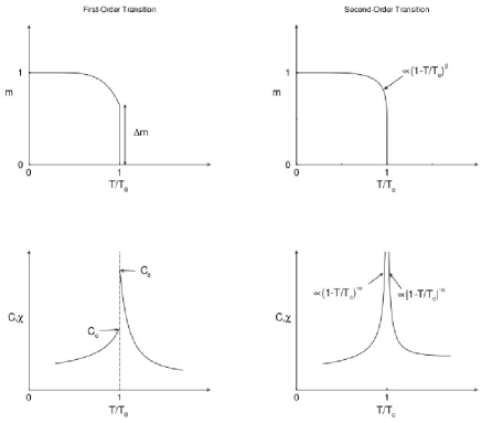
Figure 3.1: The characteristic behavior of the magnetization, $m$, specific heat $C$ and susceptibility, $\chi$ densities at first and second order phase transitions.

Of course in systems characterized by finite size, as in any numerical simulation, every statistical function like the correlation length cannot diverge and the divergences in all other quantities occurring in the infinite model are rounded and can be shifted. The example of the specific heat density for the two dimensional Ising model is illustrated in fig.3.2. The finiteness affects the scaling formulas and $\xi$ is then substituted by the linear size of the system $L$. If we write

$$t\propto\xi^{-1/\nu}\to L^{-1/\nu}$$ (3.37)

it easy to understood that the thermodynamic scaling laws $\chi\propto t^{-\gamma}$ , for finite models, has to be replaced by finite-size scaling (FFS) $\chi\propto L^{\gamma/\nu}$. In particular, [77] we obtain for the autocorrelation time a FSS of the form

$$\tau\propto L^{z}$$ (3.38)

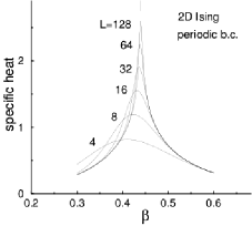
Figure 3.2: Finite size scaling behavior of the specific heat density of the $2D$ Ising model on $L\times L$ lattices close to the critical point $\beta_{c}$ .

Even for first order phase transition in a finite systems the singularities can be split in narrow peaks with height proportional to the characteristic volume $V$ and width proportional to $V^{-1}$. The system is now capable to exist in a mixed phase configurations and jump from one phase into the other, however the probability of the appearing of this mixed configurations is smoothed by the Boltzmann factor: $\textrm{exp}(2\sigma L^{n-1})$. The double-peak structure of the energy and magnetization densities that can occur for a first-order phase transition too and can be explained by the previous argumentations. For large system sizes it may require many Monte Carlo steps before the systems explore enough phase space. In fact, the autocorrelation time associated with this transitions is the inverse of the suppression factor:

$$\tau\propto\textrm{exp}(2\sigma L^{n-1})$$ (3.39)

Since in this case the autocorrelations grows exponentially with the system size, this behavior is usually called supercritical slowing down.

Chapter 4 Preparing for numerics

In this chapter will be set up all the ingredients required to implement a Monte Carlo simulation of the model treated in the chapter two. The first part will be devoted to the discretization scheme, introducing a Moyal base in which the model described by the action (2.96) on Moyal plane will be discretized. In the second part, in order to define the measurements of the conducted Monte Carlo simulation, will be applied some arguments treated in the third chapter outlining the expectation values, statistical quantities and some order parameters.

4.1 Discretization of the action

The first step across the numerical analysis is to apply a discretization scheme. Various schemes can be used like lattice approximation, but the nature of star product due to its oscillator exponential, makes the lattice approach not suitable without adaptations. We will use another discretization scheme in which our fields are approximated by finite matrices and the star product becomes the standard matrix multiplication. Our model is Euclidean, as remarked in chapter 3, the main advantage of working in this formalism is that we can establish a direct connection to statistical physic and the functional integral converges with a relatively modest statistic. The action to discretize is

$$S(\phi,\tilde{X}_{A},\tilde{X}_{B}) =\int d^{4}z\Bigg{\{}\left(\frac{\left(1-\Omega^{2}\right)^{2}}{2}-\frac{\left(1-\Omega^{2}\right)^{4}}{6\left(1+\Omega^{2}\right)^{2}}\right)\left(F^{A}_{\mu\nu}\star F^{\mu\nu}_{A}+F^{B}_{\mu\nu}\star F^{\mu\nu}_{B}\right)$$ (4.1)

$$+\left(\phi\star\bar{\phi}+\frac{4\Omega^{2}}{1+\Omega^{2}}\tilde{X}_{A}^{\mu}\star\tilde{X}_{A\mu}-\frac{\chi_{-1}}{\chi_{0}}\right)^{2}$$

$$+\left(\bar{\phi}\star\phi+\frac{4\Omega^{2}}{1+\Omega^{2}}\tilde{X}_{B}^{\mu}\star\tilde{X}_{B\mu}-\frac{\chi_{-1}}{\chi_{0}}\right)^{2}$$

$$+2(1+\Omega^{2})D_{\mu}\phi\star\overline{D_{\mu}\phi}\Bigg{\}}(z)+\mathcal{O}(\chi_{1})$$

Using the identity $D_{\mu}\phi=\phi\star\tilde{X}_{B\mu}-\tilde{X}_{A\mu}\star\phi$ we can recast the action in the following form:

$$S(\phi,\tilde{X}_{A},\tilde{X}_{B}) =\int d^{4}z\Bigg{\{}\left(\frac{\left(1-\Omega^{2}\right)^{2}}{2}-\frac{\left(1-\Omega^{2}\right)^{4}}{6\left(1+\Omega^{2}\right)^{2}}\right)\Big{(}\left[\tilde{X}_{A\mu},\tilde{X}_{A\nu}\right]_{\star}\left[\tilde{X}_{A}^{\mu},\tilde{X}_{A}^{\nu}\right]_{\star}$$ (4.2)

$$+\left[\tilde{X}_{B\mu},\tilde{X}_{B\nu}\right]_{\star}\left[\tilde{X}_{B}^{\mu},\tilde{X}_{B}^{\nu}\right]_{\star}\Big{)}+\left(\phi\star\bar{\phi}+\frac{4\Omega^{2}}{1+\Omega^{2}}\tilde{X}_{A}^{\mu}\star\tilde{X}_{A\mu}-\frac{\chi_{-1}}{\chi_{0}}\right)^{2}$$

$$+\left(\bar{\phi}\star\phi+\frac{4\Omega^{2}}{1+\Omega^{2}}\tilde{X}_{B}^{\mu}\star\tilde{X}_{B\mu}-\frac{\chi_{-1}}{\chi_{0}}\right)^{2}$$

$$+2(1+\Omega^{2})\left(\phi\star\tilde{X}_{B\mu}-\tilde{X}_{A\mu}\star\phi\right)\left(\bar{\phi}\star\tilde{X}_{A}^{\mu}-\tilde{X}_{B}^{\mu}\star\bar{\phi}\right)\Bigg{\}}(z)$$

$$+\mathcal{O}(\chi_{1})$$

As a first approach to the numerical simulation and forced by limited computation resource, we will consider the Monte Carlo simulation of the previous action around its minimum and the simulation will take $\sqrt{\frac{\chi_{-1}}{\chi_{0}}}$ as a positive parameter. In this setting the behavior of the simulations will be identical for the negative case and avoiding $\frac{\chi_{-1}}{\chi_{0}}$ to be negative we have not any problems about the thermalization. In order to define the previous action around the minimum we translate the fields $\phi$, $\tilde{X}_{A\mu}$, $\tilde{X}_{B\mu}$ using the following translated fields:

$$\phi = \psi+\sqrt{\frac{\chi_{-1}}{\chi_{0}}}\cos\alpha\textbf{I}\$$ (4.3)

$$\tilde{X}_{A\mu} = Y_{A\mu}+\frac{1}{2}\sqrt{\frac{\chi_{-1}}{\chi_{0}}}\sqrt{\frac{2\Omega^{2}}{(1+\Omega^{2})}}\textbf{I}_{\mu}\sin\alpha$$ (4.4)

$$\tilde{X}_{B\mu} = Y_{B\mu}+\frac{1}{2}\sqrt{\frac{\chi_{-1}}{\chi_{0}}}\sqrt{\frac{2\Omega^{2}}{(1+\Omega^{2})}}\textbf{I}_{\mu}\sin\alpha$$ (4.5)

Substituting the previous fields into (4.2) we get a positive action with minimum in zero:

$$S(\psi,Y_{A},Y_{B}) =\int d^{4}z\Bigg{\{}D\Big{(}\left[Y_{A\mu},Y_{A\nu}\right]_{\star}\left[Y_{A}^{\mu},Y_{A}^{\nu}\right]_{\star}+\left[Y_{B\mu},Y_{B\nu}\right]_{\star}\left[Y_{B}^{\mu},Y_{B}^{\nu}\right]_{\star}\Big{)}$$ (4.6)

$$+\left(\psi\star\bar{\psi}+\mu\cos\alpha(\psi+\bar{\psi})+CY_{A}^{\mu}\star Y_{A\mu}+\mu\textbf{I}^{\mu}Y_{A\mu}\sin\alpha\right)^{2}$$

$$+\left(\bar{\psi}\star\psi+\mu\cos\alpha(\psi+\bar{\psi})+CY_{B}^{\mu}\star Y_{B\mu}+\mu\textbf{I}^{\mu}Y_{B\mu}\sin\alpha\right)^{2}$$

$$+2(1+\Omega^{2})\left((Y_{B\mu}-Y_{A\mu})\mu\cos\alpha+\psi\star Y_{B\mu}-Y_{A\mu}\star\psi\right)$$

$$\star\left((Y_{A}^{\mu}-Y_{B}^{\mu})\mu\cos\alpha+\bar{\psi}\star Y_{A}^{\mu}-Y_{B}^{\mu}\star\bar{\psi}\right)\Bigg{\}}(z)+\mathcal{O}(\chi_{1})$$

Where for simplicity we put:

$$C=\frac{1+\Omega^{2}}{4\Omega^{2}}, D=\frac{\left(1-\Omega^{2}\right)^{2}}{2}-\frac{\left(1-\Omega^{2}\right)^{4}}{6\left(1+\Omega^{2}\right)^{2}}, \frac{\chi_{-1}}{\chi_{0}}=\mu^{2}$$ (4.7)

Recalling the first chapter we consider a Moyal base in which our fields became infinite matrices and the integral becomes a double trace, we will discretize the action introducing a cut off and then we will show how to simplify the discretization in order to conduct a feasible numerical simulations.

4.1.1 Discretization by Moyal base

The following treatment is mainly taken from [55, 29] as introduction to the Moyal base which will be used later. We can define on the algebra $\mathbb{R}_{\Theta}^{2}$ a natural basis of eigenfunctions $f_{mn}$ of the harmonic oscillator, where $m,n\in\mathbb{N}$. If we define the Hamiltonian

$$H=H_{1}+H_{2}+\cdots+H_{N},$$ (4.8)

with

$$H_{l}:=\frac{1}{2}(x^{2}_{l}+x^{2}_{l+N})\ \textrm{for}\ l=1,\cdots,N$$ (4.9)

then the $f_{mn}$ diagonalize these harmonic oscillator Hamiltonians:

$$H\star f_{mn}=\theta(m+\frac{1}{2})f_{mn},\ f_{mn}\star H_{l}=\theta(n+\frac{1}{2})f_{mn}$$ (4.10)

In order to derive $f_{mn}$ we note that the Gaussian function

$$f_{0}(x)=2e^{-\frac{1}{\theta}(x_{1}^{2}+x_{2}^{2})}$$ (4.11)

is an idempotent,

$$(f_{0}\star f_{0})(x)=4\int d^{2}y\int\frac{d^{2}k}{(2\pi)^{2}}e^{-\frac{1}{\theta}(2x^{2}+y^{2}+2x\cdot y+x\cdot\theta\cdot k+\frac{1}{4}\theta^{2}_{1}k^{2})+ik\cdot y}=f_{0}(x)$$ (4.12)

We can define the graded creation and annihilation operators

$$a=\frac{1}{\sqrt{2}}(x_{1}+ix_{2}), \frac{\partial}{\partial a}=\frac{1}{\sqrt{2}}(\partial_{1}-i\partial_{2})$$

$$\bar{a}=\frac{1}{\sqrt{2}}(x_{1}-ix_{2}), \frac{\partial}{\partial\bar{a}}=\frac{1}{\sqrt{2}}(\partial_{1}+i\partial_{2})$$ (4.13)

Computing the left and right star multiplication of this graded operator with any $f\in\mathbb{R}_{\Theta}^{2}$ we obtain

$$(a\star f)=a(x)f(x)+\frac{\theta}{2}\frac{\partial f}{\partial\bar{a}}(x), (f\star a)=a(x)f(x)-\frac{\theta}{2}\frac{\partial f}{\partial\bar{a}}(x)$$

$$(\bar{a}\star f)=\bar{a}(x)f(x)-\frac{\theta}{2}\frac{\partial f}{\partial a}(x), (f\star\bar{a})=\bar{a}(x)f(x)+\frac{\theta}{2}\frac{\partial f}{\partial a}(x)$$

The multiple application of the star multiplication for $a$ and $\bar{a}$ to $f_{0}$ leads to

$$\bar{a}^{\star n}\star f_{0}=2^{m}\bar{a}^{m}f_{0},\ f_{0}\star a^{\star n}=2^{n}a^{n}f_{0}$$ (4.15)

and

$$a\star\bar{a}^{\star m}\star f_{0} = \Bigg{\{}\begin{array}[]{cc}m\theta(\bar{a}^{\star(m-1)}\star f_{0})&\textrm{for}\ m\geq 1\\ 0&\textrm{for}\ m=0\end{array}$$ (4.18)

$$f_{0}\star a^{\star n}\star\bar{a} = \Bigg{\{}\begin{array}[]{cc}n\theta(f_{0}\star a^{\star(m-1)})&\textrm{for}\ m\geq 1\\ 0&\textrm{for}\ m=0\end{array}$$ (4.21)

with $a^{\star n}=a\star a\star\cdots\star a$ and similarly for $\bar{a}^{\star n}=\bar{a}\star\bar{a}\star\cdots\star\bar{a}$, where in the left side appear $n$ factors. Finally, can be proved by induction the following relation for $f_{mn}$:

$$f_{mn} = \frac{1}{\sqrt{n!m!\theta^{m+n}_{1}}}\bar{a}^{\star m}\star f_{0}\star a^{\star n}$$

$$= \frac{1}{\sqrt{n!m!\theta^{m+n}_{1}}}\sum^{\textrm{min}(m,n)}_{k=0}(-1)^{k}\binom{m}{k}\binom{n}{k}k!2^{m+n-2k}\theta^{k}_{1}\bar{a}^{m-k}a^{n-k}f_{0}$$

From the equations (4.12) and (4.21) we obtain the $\star$-multiplication rule:

$$(f_{mn}\star f_{kl})(x)=\delta_{nk}f_{ml}(x)$$ (4.23)

The previous multiplication rule associates the $\star$-product between $f_{ml}$ with the ordinary matrix product:

$$a(x)=\sum^{\infty}_{m,n=0}a_{mn}f_{mn}(x), b(x)=\sum^{\infty}_{m,n=0}b_{mn}f_{mn}(x)$$

$$(a\star b)(x)=\sum^{\infty}_{m,n=0}(ab)_{mn}f_{mn}(x), (ab)_{mn}=\sum^{\infty}_{k=0}a_{mk}b_{kn}$$ (4.24)

In this base we can write any elements of $\mathbb{R}_{\Theta}^{2}$ but we have to require the rapid decay [29] of the sequences of coefficients $\{a_{mn}\}$ appearing in the (4.24):

$$\sum^{\infty}_{m,n=0}a_{mn}f_{mn}(x)\in\mathbb{R}_{\Theta}^{2},\ \textrm{if},\ \sum^{\infty}_{m,n=0}\left((2m+1)^{2k}(2n+1)^{2k}|a_{mn}|^{2}\right)^{\frac{1}{2}}<\infty\ \textrm{for all}\ k.$$ (4.25)

Using again (4.12), the trace property of the integral and (4.21) we find this useful property:

$$\int d^{2}xf_{mn}(x) = \frac{1}{\sqrt{n!m!\theta^{m+n}_{1}}}\int d^{2}x(\bar{a}^{\star n}\star f_{0}\star f_{0}\star a^{\star n}(x))=\delta_{mn}\int d^{2}xf_{0}$$ (4.26)

$$= 2\pi\theta\delta_{mn}$$

The eigenfunctions $f_{nm}$ can be expressed with the help of Laguerre functions [29, 44, 72]:

$$f_{mn}(\rho,\varphi)=2(-1)^{m}\sqrt{\frac{m!}{n!}}e^{i\varphi(n-m)}\left(\sqrt{\frac{2}{\theta}}\rho\right)^{n-m}e^{-\frac{\rho^{2}}{\theta}}L_{m}^{n-m}\left(\frac{2}{\theta}\rho^{2}\right)$$ (4.27)

Our fields can be expanded in this base as:

$$X^{\mu}(x)=\sum_{m_{i},n_{i}\in\mathbb{N}}X^{\mu}_{\genfrac{}{}{0.0pt}{}{m_{1}n_{1}}{m_{2}n_{2}}}f_{m_{1}n_{1}}(x_{0},x_{1})f_{m_{2}n_{2}}(x_{2},x_{3})$$ (4.28)

and

$$\psi(x)=\sum_{m_{i},n_{i}\in\mathbb{N}}\psi_{\genfrac{}{}{0.0pt}{}{m_{1}n_{1}}{m_{2}n_{2}}}f_{m_{1}n_{1}}(x_{0},x_{1})f_{m_{2}n_{2}}(x_{2},x_{3})$$ (4.29)

Using this base we can forget the Moyal product in this way the model becomes to 9-matrix model. In view of (4.24) a $\star$-product between two fields using (4.23) can be written as

$$\Psi(x)\star\Phi(x) = \sum_{m_{i},n_{i},k_{1},l_{1}\in\mathbb{N}}\Psi_{\genfrac{}{}{0.0pt}{}{m_{1}n_{1}}{m_{2}n_{2}}}\Phi_{\genfrac{}{}{0.0pt}{}{k_{1}l_{1}}{k_{2}l_{2}}}f_{m_{1}n_{1}}(x_{0},x_{1})\star f_{k_{1}l_{1}}(x_{0},x_{1})$$ (4.30)

$$\times f_{m_{2}n_{2}}(x_{2},x_{3})\star f_{k_{2}l_{2}}(x_{2},x_{3})$$

$$= \sum_{m_{i},n_{i},k_{1},l_{1}\in\mathbb{N}}\Psi_{\genfrac{}{}{0.0pt}{}{m_{1}n_{1}}{m_{2}n_{2}}}\Phi_{\genfrac{}{}{0.0pt}{}{k_{1}l_{1}}{k_{2}l_{2}}}\delta_{n_{1}k_{1}}\delta_{n_{2}k_{2}}f_{m_{1}l_{1}}(x_{0},x_{1})f_{m_{2}l_{2}}(x_{2},x_{3})$$

$$= \sum_{m_{i},l_{1}\in\mathbb{N}}\Psi\Phi_{\genfrac{}{}{0.0pt}{}{m_{1}l_{1}}{m_{2}l_{2}}}f_{m_{1}l_{1}}(x_{0},x_{1})f_{m_{2}l_{2}}(x_{2},x_{3})$$

where

$$\Psi\Phi_{\genfrac{}{}{0.0pt}{}{m_{1}l_{1}}{m_{2}l_{2}}}=\sum_{n_{1},n_{2}\in\mathbb{N}}\Psi_{\genfrac{}{}{0.0pt}{}{m_{1}n_{1}}{m_{2}n_{2}}}\Phi_{\genfrac{}{}{0.0pt}{}{n_{1}l_{1}}{n_{2}l_{2}}}$$ (4.31)

So the star product became a ”double” matrix multiplication, the action, the equations of field and all treatments can be conducted on the infinite matrices instead directly on the continues fields. Beside, for finite matrices, the $\mathbb{N}^{2}$-indexed double sequences can be written as tensor products of ordinary matrices,

$$X_{\genfrac{}{}{0.0pt}{}{m_{1}n_{1}}{m_{2}n_{2}}}=\sum_{i=1}^{K}X^{i}_{m_{1}n_{1}}\otimes X^{i}_{m_{2}n_{2}}\;.$$ (4.32)

Since the matrix product and trace also factor into these independent components, the action factors into $S=\sum_{i=1}^{K}S(\psi^{1i},Y_{A}^{1i},Y_{B}^{1i})S(\psi^{2i},Y_{A}^{2i},Y_{B}^{2i})$. Then, regarding all $\psi^{1i},Y_{A}^{1i}$, $Y_{B}^{1i},\psi^{2i},Y_{A}^{2i},Y_{B}^{2i}$ as random variables over which to integrate in the partition function, the partition function factors, too:

$$\int\mathcal{D}(\psi^{11},Y_{A}^{11},Y_{B}^{11},\psi^{21},Y_{A}^{21},Y_{B}^{21})\cdots\mathcal{D}(\psi^{1K},Y_{A}^{1K},Y_{B}^{1K},\psi^{2K},Y_{A}^{2K},Y_{B}^{2K})\;e^{-S}$$

$$=\bigg{(}\int\mathcal{D}(\psi^{1i},Y_{A}^{1i},Y_{B}^{1i},\psi^{2i},Y_{A}^{2i},Y_{B}^{2i})\;e^{-S(\psi^{1i},Y_{A}^{1i},Y_{B}^{1i})\cdot S(\psi^{2i},Y_{A}^{2i},Y_{B}^{2i})}\bigg{)}^{K}\;.$$ (4.33)

We may therefore restrict ourselves to $K=1$ and we can split the model in 2+2 dimensions, in this way the calculus will be performed just on standard matrices. This decomposition makes the numerical treatment of 2 dimensional case simpler respect the complete one, indeed will be examined both cases. Using this base now our problem is reduced to a infinite matrix problem but is not enough to be handled numerically, we have to perform a truncation in order to obtain finite matrices, this truncation will consist in a maximum $m,n<N$ in the expansion (4.29)-(4.28). It is easy to verify that this kind of approximation corresponds in a cut in energy, in fact recalling the definition (4.10) of $f_{mn}$ we have:

$$\{H,f_{mn}\}_{\star}=\theta(m+n+\frac{1}{2})f_{mn}(\varphi,\rho)$$ (4.34)

Beside, the functions $f_{mn}$ with $m,n<N$ induce a cut-off in position space and momentum space, indeed the function

$$L_{m}^{\alpha}(z)z^{\alpha/2}e^{-z/2}$$ (4.35)

with $z=\frac{2}{\theta}\rho^{2}$, is rapidly decreasing beyond the last maximum $(z^{\alpha}_{m})_{max}$. Numerically can be found $(z^{\alpha}_{m})_{max}<2\alpha+4m$ and thus the radial cut-off

$$\rho_{max}\sim\sqrt{2\theta}\ ,\ \textrm{for}\ m,n<N$$ (4.36)

In addition, for $p_{1}=−p\sin\psi$, $p_{2}=p\cos\psi$ we obtain [59] using (4.27) ,

$$\tilde{f}_{mn}(p,\psi) = \int_{0}^{\infty}\rho d\rho\int_{0}^{2\pi}e^{ip\rho\sin(\varphi-\psi)}f_{mn}(\rho,\varphi)$$ (4.37)

$$= 4\pi(-1)^{n}\sqrt{\frac{m!}{n!}}e^{i\psi(n-m)}\int_{0}^{\infty}d\rho\left(\sqrt{\frac{\theta}{2}}p\right)^{n-m}L_{m}^{n-m}\Big{(}\frac{\theta}{2}p^{2}\Big{)}J_{n-m}(\rho p)e^{-\frac{\rho^{2}}{\theta}}$$

$$= 2\pi\theta\sqrt{\frac{m!}{n!}}e^{i(\phi+\pi)(n-m)}\left(\sqrt{\frac{\theta}{2}}p\right)^{n-m}L_{m}^{n-m}\Big{(}\frac{\theta}{2}p^{2}\Big{)}e^{-\frac{\theta}{4}p^{2}}$$

In the end we obtain

$$p_{max}\sim\sqrt{\frac{8N}{\theta}}\,\ \textrm{for}\ m,n<N$$ (4.38)

Summarizing, to operate the discretization we have the following correspondences:

$$\phi(x)\in\mathbb{R}_{\Theta}^{4} \rightarrow \hat{\phi}\in\mathbb{M}_{N}$$ (4.39)

$$Y^{A}_{\mu}(x)\in\mathbb{R}_{\Theta}^{4} \rightarrow \hat{Y}^{A}_{\mu}\in\mathbb{M}_{N}$$ (4.40)

$$Y^{B}_{\mu}(x)\in\mathbb{R}_{\Theta}^{4} \rightarrow \hat{Y}^{B}_{\mu}\in\mathbb{M}_{N}$$ (4.41)

$$\int a(x)dx \rightarrow \textrm{Tr}(\hat{a})$$ (4.42)

After truncating the representative matrices is convenient to operate another substitution [71]:

$$Z_{0}=\hat{Y}^{A}_{0}+i\hat{Y}^{A}_{1}, \bar{Z}_{0}=\hat{Y}^{A}_{0}-i\hat{Y}^{A}_{1}$$

$$Z_{1}=\hat{Y}^{B}_{0}+i\hat{Y}^{B}_{1}, \bar{Z}_{1}=\hat{Y}^{B}_{0}-i\hat{Y}^{B}_{1}$$

$$Z_{2}=\hat{Y}^{A}_{2}+i\hat{Y}^{A}_{2}, \bar{Z}_{2}=\hat{Y}^{A}_{2}-i\hat{Y}^{A}_{3}$$

$$Z_{3}=\hat{Y}^{B}_{2}+i\hat{Y}^{B}_{3}, \bar{Z}_{3}=\hat{Y}^{B}_{2}-i\hat{Y}^{B}_{3}$$ (4.43)

Implementing the previous replacements for the two dimensional model, thus using only $Z_{0}$, $Z_{1}$, in eq. (4.6) we arrive at

$$\\ S_{2}=\operatorname{Tr}\left(\mathcal{L}_{F}+\mathcal{L}_{V_{0}}+\mathcal{L}_{V_{1}}+\mathcal{L}_{D_{0}}\bar{\mathcal{L}}_{D_{0}}+\mathcal{L}_{D_{1}}\bar{\mathcal{L}}_{D_{1}}\right)$$ (4.44)

with

$$\mathcal{L}_{2F} = \frac{D}{2}\left(\left[\bar{Z}_{0},Z_{0}\right]^{2}+\left[\bar{Z}_{1},Z_{1}\right]^{2}\right)$$

$$\mathcal{L}_{2V_{0}} = \left(\psi\bar{\psi}+\mu\cos\alpha(\psi+\bar{\psi})+\frac{1}{2}\left\{\bar{Z}_{0},Z_{0}\right\}+\frac{\mu\sin\alpha}{\sqrt{2C}}((-1+i)Z_{0}+(1+i)\bar{Z}_{0})\right)^{2}$$

$$\mathcal{L}_{2V_{1}} = \left(\bar{\psi}\psi+\mu\cos\alpha(\psi+\bar{\psi})+\frac{1}{2}\left\{\bar{Z}_{1},Z_{1}\right\}+\frac{\mu\sin\alpha}{\sqrt{2C}}((-1+i)Z_{1}+(1+i)\bar{Z}_{1})\right)^{2}$$

$$\mathcal{L}_{2D_{0}} = \sqrt{2(1+\Omega^{2})}\left(\mu\cos\alpha(Z_{1}+\bar{Z}_{1}-Z_{0}-\bar{Z}_{0})+\psi(Z_{1}+\bar{Z}_{1})-(Z_{0}+\bar{Z}_{0})\psi\right)$$

$$\mathcal{L}_{2D_{1}} = \sqrt{2(1+\Omega^{2})}\left(\mu\cos\alpha(Z_{1}-\bar{Z}_{1}-Z_{0}+\bar{Z}_{0})+\psi(Z_{1}-\bar{Z}_{1})-(Z_{0}-\bar{Z}_{0})\psi\right)$$

Where for simplicity we have omitted the hat on the matrices and the bars stand for the hermitian conjugate. With this discretized action (4.44), the scalar $\psi$ and the gauge fields $Z_{0}$, $Z_{1}$ become 3-complex matrix instead to have one complex matrix for the scalar and four real matrices for the $Y_{A\mu}$, $Y_{B\mu}$ fields. In this setting the algorithm for Monte Carlo simulation becomes simpler especially with the update algorithm used here. In the four dimensional model it is convenient to use the (4.43) too, in this case there are some additional terms. In particular appear the crossed commutators between the $Z_{i}$ in the Y-M part:

$$S_{4}=\operatorname{Tr}\left(\mathcal{L}_{F}+\mathcal{L}_{V_{0}}+\mathcal{L}_{V_{1}}+\mathcal{L}_{D_{0}}\bar{\mathcal{L}}_{D_{0}}+\mathcal{L}_{D_{1}}\bar{\mathcal{L}}_{D_{1}}+\mathcal{L}_{D_{2}}\bar{\mathcal{L}}_{D_{2}}+\mathcal{L}_{D_{3}}\bar{\mathcal{L}}_{D_{3}}\right)$$ (4.45)

With

$$\mathcal{L}_{4F} = \frac{D}{2}\Big{(}\left[\bar{Z}_{0},Z_{0}\right]^{2}+\left[\bar{Z}_{1},Z_{1}\right]^{2}+\frac{1}{4}\Big{(}\left[Z_{0}+\bar{Z}_{0},Z_{2}-\bar{Z}_{2}\right]^{2}-\left[Z_{0}+\bar{Z}_{0},Z_{2}+\bar{Z}_{2}\right]^{2}$$

$$+ \left[Z_{0}-\bar{Z}_{0},Z_{2}+\bar{Z}_{2}\right]^{2}-\left[Z_{0}-\bar{Z}_{0},Z_{2}-\bar{Z}_{2}\right]^{2}-\left[Z_{1}+\bar{Z}_{1},Z_{3}+\bar{Z}_{3}\right]^{2}$$

$$+ \left[Z_{1}+\bar{Z}_{1},Z_{3}-\bar{Z}_{3}\right]^{2}+\left[Z_{1}-\bar{Z}_{1},Z_{3}+\bar{Z}_{3}\right]^{2}-\left[Z_{1}-\bar{Z}_{1},Z_{3}-\bar{Z}_{3}\right]^{2}\Big{)}\Big{)}$$

$$\mathcal{L}_{4V_{0}} = \big{(}\psi\bar{\psi}+\mu\cos\alpha(\psi+\bar{\psi})+\frac{1}{2}\left(\left\{\bar{Z}_{0},Z_{0}\right\}+\left\{\bar{Z}_{2},Z_{2}\right\}\right)$$

$$+ \frac{\mu\sin\alpha}{2\sqrt{C}}((-1+i)(Z_{0}+Z_{2})+(1+i)(\bar{Z}_{0}+\bar{Z}_{2}))\big{)}^{2}$$

$$\mathcal{L}_{4V_{1}} = \big{(}\bar{\psi}\psi+\mu\cos\alpha(\psi+\bar{\psi})+\frac{1}{2}\left(\left\{\bar{Z}_{1},Z_{1}\right\}+\left\{\bar{Z}_{3},Z_{3}\right\}\right)$$

$$+ \frac{\mu\sin\alpha}{2\sqrt{C}}((-1+i)(Z_{1}+Z_{3})+(1+i)(\bar{Z}_{1}+\bar{Z}_{3}))\big{)}^{2}$$

$$\mathcal{L}_{4D_{0}} = \sqrt{2(1+\Omega^{2})}\left(\mu\cos\alpha(Z_{1}+\bar{Z}_{1}-Z_{0}-\bar{Z}_{0})+\psi(Z_{1}+\bar{Z}_{1})-(Z_{0}+\bar{Z}_{0})\psi\right)$$

$$\mathcal{L}_{4D_{1}} = \sqrt{2(1+\Omega^{2})}\left(\mu\cos\alpha(Z_{1}-\bar{Z}_{1}-Z_{0}+\bar{Z}_{0})+\psi(Z_{1}-\bar{Z}_{1})-(Z_{0}-\bar{Z}_{0})\psi\right)$$

$$\mathcal{L}_{4D_{2}} = \sqrt{2(1+\Omega^{2})}\left(\mu\cos\alpha(Z_{3}+\bar{Z}_{3}-Z_{2}-\bar{Z}_{2})+\psi(Z_{3}+\bar{Z}_{3})-(Z_{2}+\bar{Z}_{2})\psi\right)$$

$$\mathcal{L}_{4D_{3}} = \sqrt{2(1+\Omega^{2})}\left(\mu\cos\alpha(Z_{3}-\bar{Z}_{1}-Z_{2}+\bar{Z}_{2})+\psi(Z_{3}-\bar{Z}_{3})-(Z_{2}-\bar{Z}_{2})\psi\right)$$

In this case the action (4.44) becomes 5 complex matrix model instead eight real matrices $Y_{A\mu}$, $Y_{B\mu}$ and one complex matrix $\psi$. This form may seem cumbersome but it still more comfortable for numerical simulations. The next step is to define the estimator for the average values of interest and to develop some numerical parameters in order to analyze the numerical results.

4.2 Definition of the observables

Calling $(\psi,Z_{i})$ a configuration of the fields (where $i=1,2$ for the two dimensional case and $i=1,\cdots,4$ for the four dimensional one), the probability to encounter this configuration is given by

$$P[(\psi,Z_{i})]=\frac{e^{-S[(\psi,Z_{i})]}}{\mathcal{Z}}$$ (4.46)

where $S[(\psi,Z_{i})]$ is the action (4.44) or (4.45) of the system evaluated in the particular configuration and $\mathcal{Z}$ is the partition function:

$$\mathcal{Z}=D[(\psi,Z_{i})]e^{-S[(\psi,Z_{i})]}$$ (4.47)

$D[(\psi,Z_{i})]$ denotes the integration over all field configurations. The expectation value of the observable $O$ is defined by the expression:

$$\langle O\rangle=\int D[(\psi,Z_{i})]\frac{e^{-S[(\psi,Z_{i})]}O[(\psi,Z_{i})]}{\mathcal{Z}}$$ (4.48)

Following Monte Carlo methods, will be produced a sequence of configurations $\{(\psi,Z_{i})_{j}\},j=1,2,\cdots,T_{MC}$ and evaluated the average of the observables over that set of configurations. The sequences of configurations obtained, a Monte Carlo chain, are representations of the configuration space at the given parameters. In this frame the expectation value is approximated as

$$\langle O\rangle\approx\frac{1}{T_{MC}}\sum_{j=1}^{T_{MC}}O_{j}$$ (4.49)

where $O_{j}$ is the value of the observable $O$ evaluated in the $j$-sampled configuration, $(\psi,Z_{i})_{j}$, $O_{i}=O[(\psi,Z_{i})_{j}]$.

4.2.1 Energy and specific heat

The internal energy is defined as:

$$E(\Omega,\mu,\alpha)=\langle S\rangle$$ (4.50)

and the specific heat takes the form

$$C(\Omega,\mu,\alpha)=\langle S^{2}\rangle-\langle S\rangle^{2}$$ (4.51)

These terms correspond to the usual definitions for energy

$$E(\Omega,\mu,\alpha)=-\frac{1}{\mathcal{Z}}\frac{\partial\mathcal{Z}}{\partial\beta}$$ (4.52)

and specific heat

$$C(\Omega,\mu,\alpha)=\frac{\partial E}{\partial\beta}$$ (4.53)

where $\mathcal{Z}$ is the partition function. It is very useful to compute separately the average values of the four contributions:

$$S_{F}(\psi,Z_{i}) = \operatorname{Tr}\mathcal{L}_{F}$$ (4.54)

$$S_{V_{0}}(\psi,Z_{i}) = \operatorname{Tr}\mathcal{L}_{V_{0}}$$ (4.55)

$$S_{V_{1}}(\psi,Z_{i}) = \operatorname{Tr}\mathcal{L}_{V_{1}}$$ (4.56)

$$S_{D}(\psi,Z_{i}) = \operatorname{Tr}\left(\mathcal{L}_{D_{j}}\bar{\mathcal{L}}_{D^{j}}\right)$$ (4.57)

Where $i,j=1,2$ or $i,j=1,\cdots,4$. The corresponding expectation values to (4.54)-(4.57) are

$$F(\Omega,\mu,\alpha) = \langle S_{F}\rangle$$ (4.58)

$$V_{0}(\Omega,\mu,\alpha) = \langle S_{V_{1}}\rangle$$ (4.59)

$$V_{1}(\Omega,\mu,\alpha) = \langle S_{V_{1}}\rangle$$ (4.60)

$$D(\Omega,\mu,\alpha) = \langle S_{D}\rangle$$ (4.61)

$$V = V_{0}+V_{1}$$ (4.62)

4.2.2 Order parameters

The previous quantities are not enough if we want to measure the various contributions of different modes of the fields to the configuration $\psi,Z_{i}$. Therefore we need some control parameters usually called order parameters. As a first idea we can think about a quantity related to the norms of the fields for example the sums $\sum_{nm}|\psi_{nm}|^{2}$, $\sum_{nm}|Z_{inm}|^{2}$ of all squared entries of our matrices, this quantity is called the full power of the field [81, 82] and it can be computed as the trace of the square:

$$\varphi^{2}_{a} = \operatorname{Tr}(|\psi|^{2})$$ (4.63)

$$Z^{2}_{ia} = \operatorname{Tr}(|Z_{i}|^{2})$$ (4.64)

This parameter turns to be very useful to find the region where the configurations are considered disordered for which we expect to have a random distribution of the modes $\langle\varphi^{2}_{a}\rangle\sim 0$, $\langle Z^{2}_{ia}\rangle\sim 0$ and the so called ordered phase in which we have $\langle\varphi^{2}_{a}\rangle>>0$, $\langle Z^{2}_{ia}\rangle>>0$. The full power of the field can be used to determine for which independent parameters there is a transition between the disordered and ordered regime. However $\langle\varphi_{a}\rangle$ alone is not a real order parameter because does not distinguish contributions from the different modes but we can use it as a reference to define the quantities:

$$\varphi^{2}_{0} = \sum^{N}_{n=0}|a_{nn}|^{2}$$

$$Z^{2}_{i0} = \sum^{N}_{n=0}|z_{inn}|^{2}$$ (4.65)

Referring to the base (4.27) it is easy to see that such parameters are connected to the pure spherical contribution. This quantity will be used to analyze the spherical contribution to the full power of the field. We can define the corresponding susceptibility as:

$$\chi_{\varphi_{0}} = \langle\varphi_{0}^{2}\rangle-\langle\varphi_{0}\rangle^{2}$$

$$\chi_{Z_{i0}} = \langle Z^{2}_{i0}\rangle-\langle Z_{i0}\rangle^{2}$$ (4.66)

We can generalize the previous quantity defining some parameters $\varphi_{l}$ in such a way they form a decomposition of the full power of the fields.

$$\varphi^{2}_{a}=\varphi^{2}_{0}+\sum_{l}\varphi^{2}_{l},\ Z_{ia}^{2}=Z_{i0}^{2}+\sum_{l}Z_{il}^{2}$$ (4.67)

Following this prescription the other quantity for $l>0$ can be defined as:

$$\varphi^{2}_{l}=\sum^{l}_{n,m=0}|a_{nm}(1-\delta_{nm})|^{2},\ Z_{il}^{2}=\sum^{l}_{n,m=0}|z_{lnm}(1-\delta_{nm})|^{2}$$ (4.68)

If the contribution is dominated from the spherical symmetric parameter we expect to have $\langle\varphi^{2}_{a}\rangle\sim\langle\varphi^{2}_{0}\rangle$, $\langle Z_{ia}^{2}\rangle\sim\langle Z^{2}_{i0}\rangle$. In this regime for the uniform ordered region we have $\langle\varphi^{2}_{0}\rangle\sim 0$, $\langle Z_{i0}^{2}\rangle\sim 0$ and in the disordered phase we expect $\langle\varphi^{2}_{l}\rangle\sim 0$, $\langle Z_{il}^{2}\rangle\sim 0$ for all $l$. With (4.68) we can define the order parameters $\varphi^{2}_{1}$, $Z_{i1}^{2}$ as a particular case $l=1$ we have

$$\varphi^{2}_{1}=|a_{10}|^{2}+|a_{01}|^{2},\ Z_{i1}^{2}=|z_{i10}|^{2}+|z_{i01}|^{2}$$ (4.69)

and its susceptibility,

$$\chi_{\varphi_{1}}=\langle\varphi_{1}^{2}\rangle-\langle\varphi_{1}\rangle^{2},\ \chi_{Z_{i1}}=\langle Z_{i1}^{2}\rangle-\langle Z_{i1}\rangle^{2}$$ (4.70)

In the next simulations we be evaluated the quantities related to $l=0$ and to $l=1$ as representative of those contribution where the rotational symmetry is broken. A region characterized by $\langle\varphi^{2}_{1}\rangle>>0$, $\langle Z_{i1}^{2}\rangle>>0$ is called [81] non-uniform, such region feature a large contributions in which the spherical symmetry is broken. Using higher $l$ in (4.68) we can analyze the contributions of the remaining modes, but turns out that the measurements of the first two modes are enough to characterize the behavior of the system.

Chapter 5 Numerical results

This last chapter is devoted to present the numerical results of the 4-dimensional and 2-dimensional model constructed and approximated in the previous chapters. In the first part will be discussed the behaviors of the defined observables of the full 4-dimensional model varying the parameters. Meanwhile in the second part will be showed the result for the 2-dimensional model for the same values of parameters and compared with the full model results.

5.1 Four dimensional case

Now we are ready to discuss the results of the Monte Carlo simulation on the approximated spectral model described in the chapter 2 and discretized in the previous chapter. As a first approach to Monte Carlo simulation of such kind of model, we use some restrictions on the parameters. Will be used the spectral action around its minimum (4.45) in order to simplify the calculation, in this frame in the action is symmetric under the transformation $\mu\to-\mu$ so will be used the condition $\mu\geq 0$ and $\mu^{2}\geq 0$. Will be explored the range $\mu\in[0,3]$, this interval was chosen in such a way to show a particular behavior of the system for fixed $\Omega$. The parameter $\Omega$ appears only with its square and is defined as a real parameter, therefore for the $\Omega$ too we require $\Omega\geq 0$. Beside, if we refer to the scalar model, is possible to prove [44] using the Langmann-Szabo duality [17], that the model can be fully described varying $\Omega$ in the range $[0,1]$, for higher $\Omega$ the system can be remap inside the previous interval. In the present model the L-S duality does not hold any more, but forced by limited resource, we conjecture that the interval $\Omega\in[0,1]$ still enough to describe the system. The last parameter to consider is $\alpha$, it is connected to the choice of the vacuum state, of course, the range of $\alpha$ is $[0,2\pi]$. The study of the system varying this parameter is quite important; from a theoretical point of view, because is related to the vacuum invariance and for numerical reasons too. In fact, in the action of both 4-dimensional and 2-dimensional model appear some contributions $\sim(\sin\alpha)/\Omega$ which seem to diverge for $\Omega=0$, numerically we have verified that is an eliminable divergence and the curves of the observables can be extended in zero by continuity. Nevertheless, this factor slow down the computations due to its high value close to $\Omega=0$. Studying the dependence on $\alpha$ we can conclude that in the limit $N\to\infty$ the observables are independent from $\alpha$, therefore for our purposes $\alpha$ will be fixed equal to zero avoiding the annoying terms. In general for each observable are computed the graphs for $N=$5, 10, 15, 20 matrix size.

5.1.1 Varying $\alpha$

We start looking at the variation of energy density and the full power of the fields density for fixed $\mu$ and $\Omega$, varying $\alpha\in[0,2\pi]$. As representative here will be presented the graphs for $\mu=1$, $\Omega=\{1,0.5\}$ but we obtain the same behaviors for any other choice of the parameters allowed in the range considered.

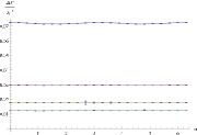
Figure 5.1: Total energy density and full power of the fields density for $\varphi^{2}_{a}$, $Z_{0a}^{2}$ (from the left to the right) fixing $\mu=1$, $\Omega=1$, varying $\alpha$ and $N$. $N=5$ (blue), $N=10$ (purple), $N=15$ (brown), $N=20$ (green).

All tree graphs show an oscillating behavior of the values, this oscillation is present in all other quantities measured. The amplitude of this oscillation becomes smaller and smaller increasing the size of the matrix and this is true for all the quantity measured. The same trend is described in fig.5.2 in which position of the maximum are different but the amplitudes become smaller increasing $N$

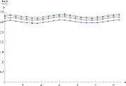
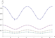
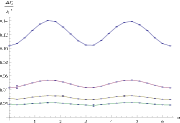
Figure 5.2: Total energy density and full power of the fields density for $\varphi^{2}_{a}$, $Z_{0a}^{2}$ (from the left to the right) fixing $\mu=1$, $\Omega=0.5$, varying $\alpha$ and $N$.

This results allow us to consider $\alpha=0$ for all next graphs, since we are interested in the behavior of the system for $N\to\infty$. This occurrence simplify all the next simulations thanks to the vanishing the of terms $\sim(\sin\alpha)/\Omega$ appearing in the discretized action. Beside, such results induce us to reckon the parameter $\alpha$ as connected to the remaining invariance of the vacuum state for the exact model.

5.1.2 Varying $\Omega$

Now we will analyze three cases in which $\mu$ is fixed to $0,1,3$, $\alpha$ is zero and we vary $\Omega\in[0,1]$. Will be showed the results of simulation for matrix size of 5, 10, 15, 20. In the rest of this chapter we ignore for the computation of $E,D,V,F$ the prefactor $(1+\Omega^{2})$. In this way we focus our attention to the integral as the source of possible phase transitions.

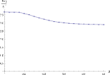
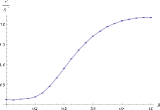
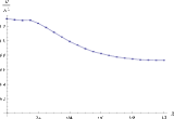
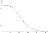
Figure 5.3: Total energy density and the various contributions for $\mu=1$. From the left to the right the density for: E, V, D, F.

The graphs in fig.5.3 show the total energy density $\langle S\rangle/N^{2}$ and the various contributions: the potential $V/N^{2}$, the Yang-Mills part $F/N^{2}$ and the covariant derivative part $D/N^{2}$, for $\mu=1$ $\alpha=0$ defined in the previous chapter. There is no evident discontinuity or peak, apart a small deviation visible in the origin, but we can interpret it as a finite volume effect. Increasing the size of the matrices the curves and the apparent discontinuity close to zero become smoother fig.5.4.

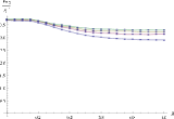
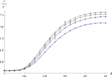
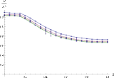
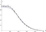
Figure 5.4: Total energy density and the various contributions for $\mu=1$, $\alpha=0$ varying $\Omega$ and $N$. From the left to the right $E$, $V$, $D$, $F$ with $N=5$ (blue), $N=10$ (purple), $N=15$ (brown), $N=20$ (green).

Comparing the energy density and the various contributions fig.5.5 we notice that the contributions between $F$ and $V$ balance each other and the total energy follows the slope of $D$, this behavior continues increasing the size of the matrices fig.5.5.

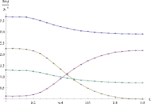
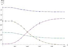
Figure 5.5: Comparison of the total energy density and the various contributions for $\mu=1$, $\alpha=0$. $E$ (blue), $F$ (brown), $D$ (green), $V$ (purple). With $N=5$ (left) and $N=20$ (right).

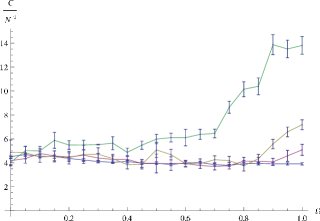
Figure 5.6: Specific heat for $\mu=1$.

The specific heat density defined as $(\langle S\rangle^{2}-\langle S^{2}\rangle)/N^{2}$ shows fig.5.6 a peak in $\Omega=1$, this peak increases as $N$ increase. This behavior is typical of a phase transition and the peak is not clear for small $N$ due to the finite volume effect. In order to gain some informations on the composition of the fields we look at the order parameters defined in the previous chapter. Starting from $\psi$ field, in the figure 5.6 it is showed the graphs for $\varphi_{a}^{2}$, $\varphi^{2}_{0}$ and $\varphi^{2}_{1}$ for $N=5$.

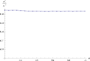
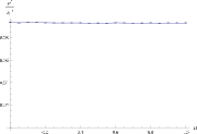
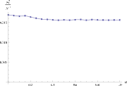
Figure 5.7: From the left to the right $\varphi_{a}^{2}$, $\varphi^{2}_{0}$ and $\varphi^{2}_{1}$ for $\mu=1$ varying $\Omega$

The three values $\varphi_{a}^{2}$, $\varphi^{2}_{0}$ and $\varphi^{2}_{1}$ seem essentially constant, comparing the three graphs fig.5.7 it is easy to see the dominance of the spherical contribution $\varphi^{2}_{0}$ to the full power of the field.

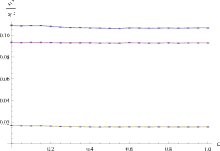
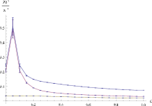
Figure 5.8: On the left comparison of $\varphi_{a}^{2}$ (blue), $\varphi^{2}_{0}$ (purple) and $\varphi^{2}_{1}$ (green) density. On the right comparison of $Z_{0a}^{2}$ (blue), $Z_{00}^{2}$ (purple) and $Z_{01}^{2}$ (green) density.

The behavior of the $Z_{0}$ fields is different, referring to figure 5.8 where are showed the quantity $Z_{0a}^{2}$, $Z_{00}^{2}$ and $Z_{01}^{2}$ over $N^{2}$, the spherical contribution becomes dominant approaching to $\Omega=0$ starting from a zone in which the contribution of $Z_{00}^{2}$ and $Z_{01}^{2}$ are comparable. For brevity will not be showed only the graphs for $Z_{0a}^{2}$, $Z_{00}^{2}$ and $Z_{01}^{2}$ but taking in account the statistical errors the other $Z_{i}$ related graphs appear compatible to the $Z_{0}$ case. The dependence of the previous quantities on $N$ are showed in the following graphs fig.5.9.

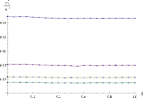
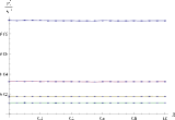
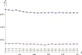
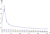
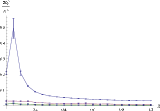
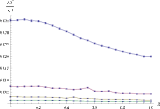
Figure 5.9: Starting from the up left corner and from the left to the right the densities for $\varphi_{a}^{2}$, $\varphi^{2}_{0}$, $\varphi^{2}_{1}$, $Z_{0a}^{2}$, $Z_{00}^{2}$ and $Z_{01}^{2}$ for $\mu=1$ varying $\Omega$ and $N$.

The values of the quantity of all the previous parameters decreases with $N$ but the dominance of the $\varphi_{0}$ on the total power of the field is independent by $N$. The peak related to $Z_{0}$ decrease, but if look at the single graph for $N=20$ the spherical contribution approaching the point $\Omega=0$ features a peak.

Now we will analyze the model for $\mu=0$; fig.5.10 shows the graphs for total energy density and the contributions $V$, $D$, $F$. The slope of the total energy density seems to be constant. The $D$ contribution and the $F$ do not balance each other like in the previous case, but all the three contributions balance among them self to produce a constant sum.

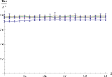
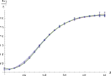
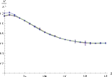
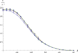
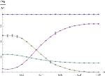
Figure 5.10: Total energy density, various contributions and the comparison among them for $\mu=0$ varying $\Omega$ and $N$. From the left to the right $E$, $V$, $D$, $F$ and comparison.

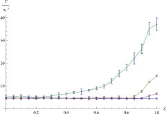
Figure 5.11: Specific heat density for $\mu=0$ varying $\Omega$ and $N$.

The specific heat density shows fig.5.11 again the peak in $\Omega=1$ as $N$ increase. For the other quantities $\varphi_{a}^{2}$, $\varphi^{2}_{0}$, $\varphi^{2}_{1}$ and $Z_{0a}^{2}$, $Z_{00}^{2}$, $Z_{01}^{2}$ we have the same behavior fig.5.14 of $\mu=1$ case, except for the oscillation appearing in the $Z_{0a}^{2}$, $Z_{00}^{2}$ graphs close to zero, anyway it appears only for $N=5$.

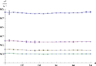
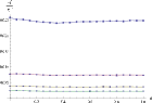
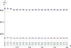
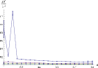
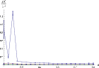
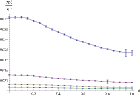
Figure 5.12: Starting from the up left corner and from the left to the right the densities for $\varphi_{a}^{2}$, $\varphi^{2}_{0}$, $\varphi^{2}_{1}$, $Z_{0a}^{2}$, $Z_{00}^{2}$ and $Z_{01}^{2}$ for $\mu=0$ varying $\Omega$ and $N$.

A complete different response of the system is described in the graphs for $\mu=3$, as we can see from fig.5.13. The slope of total energy density is very similar to the $F$ component instead $D$. Beside, appears a maximum around $\Omega=0.4$ for $N\to\infty$. This dramatic change of the graphs might be interpreted as consequence of a phase transition ruled by the parameter $\mu$, actually in the next section we will find a peak in the specific heat density for some fixed $\Omega$ and varying $\mu\in[0,3]$.

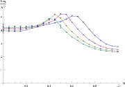
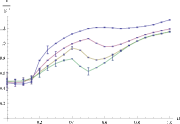
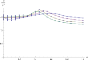
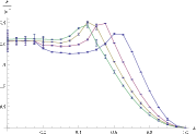
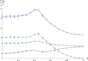
Figure 5.13: Total energy density, various contributions and the comparison among them for $\mu=3$ varying $\Omega$ and $N$. From the left to the right $E$, $V$, $D$, $F$ and comparison.

Specific heat density displays fig.5.14 this change too, in fact instead the peak in $\Omega=1$, it appears in the opposite side of the studied interval in $\Omega=0$. This peak too, due to its grows increasing $N$ indicates a phase transition.

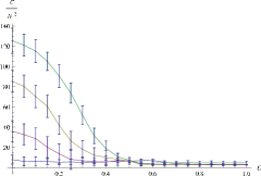
Figure 5.14: Specific heat density for $\mu=3$ varying $\Omega$ and $N$.

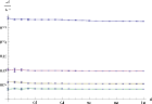
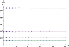
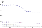
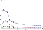
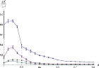
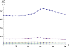
Figure 5.15: Starting from the up left corner and from the left to the right the densities for $\varphi_{a}^{2}$, $\varphi^{2}_{0}$, $\varphi^{2}_{1}$, $Z_{0a}^{2}$, $Z_{00}^{2}$ and $Z_{01}^{2}$ for $\mu=3$ varying $\Omega$ and $N$.

The fig.5.15 describes the behavior of the order parameters densities $\varphi_{a}^{2}$, $\varphi^{2}_{0}$, $\varphi^{2}_{1}$ and $Z_{0a}^{2}$, $Z_{00}^{2}$, $Z_{01}^{2}$, they have a similar aspect to the previous relative graphs. For the $\psi$ field the spherical contribution remains dominant, beside in the $\varphi^{2}_{1}$ graph appears a deviation from the constant slope this deviation is evident for $N=5$ but still there for higher $N$. The order parameters for $Z_{0}$ display a peak close to the origin without oscillations even for $N=5$. This maximum for higher $N$ does not move closer to the origin, in other words, this shift in not due to the finite volume effect. Even for $Z^{2}_{01}$ graph appears a deviation from the constant slope, a small peak which becomes shifted and smoother for higher $N$

5.1.3 Varying $\mu$

In this section is analyzed the response of the system varying $\mu\in[0,3]$ where $\Omega$ is fixed to $0,0.5,1$ and $\alpha$ is always zero. We start displaying the graphs fig.5.16 of the total energy density and of various contributions for $\Omega=0$. There is no evident discontinuity but appears a peak in the total energy density around $\mu\approx 2.5$ for $N=20$. Comparing all the contributions is easy to notice that the slope of the total energy is dictated by the curve $V$ of the potential part.

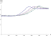
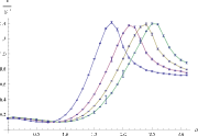
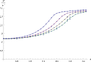
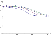
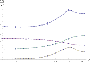
Figure 5.16: The total energy density and the various contributions for $\Omega=0$ varying $\mu$ and $N$. From the left to the right $E$, $V$, $D$, $F$ an comparison with $N=5$ (blue), $N=10$ (purple), $N=15$ (brown), $N=20$ (green). For the comparison: $E$ (blue), $V$ (purple), $D$ (brown), $F$ (green).

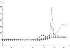
Figure 5.17: Specific heat density for $\Omega=0$ varying $\mu$ and $N$.

As mentioned before, the specific heat density fig.5.17 features a peak around $\mu\approx 2.5$ for $N=20$ and again, due to this behavior as $N$ increase, we could relate this peak to a phase transition. The plots for the quantities $\varphi_{a}^{2}$ and $\varphi^{2}_{0}$ denote a strong dependence on $\mu$, in particular the slope of $\varphi^{2}_{0}$ seems mostly linear, for $\varphi^{2}_{1}$ we notice a similar behavior but the slope is no longer linear. Comparing the three graphs fig.5.18 we deduce that close to the origin the non spherical contribution is bigger the spherical one, increasing $\mu$ this situation capsizes and $\varphi^{2}_{0}$ becomes dominant respect $\varphi^{2}_{1}$.

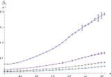
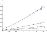
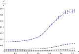
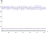
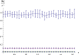
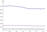
Figure 5.18: Starting from the up left corner and from the left to the right the densities for $\varphi_{a}^{2}$, $\varphi^{2}_{0}$, $\varphi^{2}_{1}$, $Z_{0a}^{2}$, $Z_{00}^{2}$ and $Z_{01}^{2}$ for $\Omega=0$ varying $\mu$ and $N$.

The behavior of the $Z_{0}$ fields is quite different, referring to figure 5.18, the spherical contribution is always dominant for the all interval $\mu\in[0,3]$. The curves for $Z_{0a}^{2}$, $Z_{00}^{2}$ are compatible to the constant slope, for $Z_{01}^{2}$ we have the same dependence on $\mu$ in particular there is a smooth descending step, however this step becomes smoother for bigger $N$. It is behooves to say that due to some cancellations effects the statistical errors are quite big and they can hide some dependence, anyway this results tell us about the dependence of the order parameter for $Z_{i}$ and in general of the system, on the two choice $\Omega=0$ or $\Omega\neq 0$.

Now we will analyze the model for $\Omega=0.5$; as fig.5.19 shows the graphs have a different slope comparing to the previous case, the maximum of total energy density follow the one of the $V$ component. If we focus ourself only on the total energy graph and we compare it with the one for $\Omega=0$, we notice a shift of the maximum for each $N$. In particular in fig.5.19 some maximum are moved outside the studied interval.

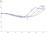
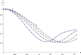
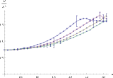
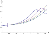
Figure 5.19: Total energy density and contributions for $\Omega=0.5$ varying $\mu$ and $N$. From the left to the right $E$, $V$, $D$, $F$.

We can find this shift very clearly looking at specific heat density graph fig.5.20, we find again the peak as $N$ increase but it is shifted around $\mu\approx 3.3$.

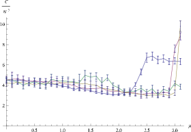
Figure 5.20: Specific heat density for $\Omega=0.5$ varying $\mu$ and $N$.

The graphs fig.5.23 for $\varphi_{a}^{2}$, $\varphi^{2}_{0}$ have the same behavior of $\Omega=0.5$ case, excluding some fluctuations close to the origin for $N=5$ due to the finite volume effect, $\varphi^{2}_{1}$ graph displays an almost constant curve. However, close to the origin, the spherical contribution and the first non spherical one are comparable.

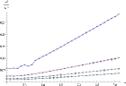
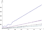
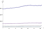
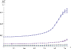
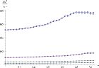
Figure 5.21: Starting from the up left corner and from the left to the right the densities for $\varphi_{a}^{2}$, $\varphi^{2}_{0}$, $\varphi^{2}_{1}$, $Z_{0a}^{2}$, $Z_{00}^{2}$ and $Z_{01}^{2}$ for $\Omega=0.5$ varying $\mu$ and $N$.

The introduction of $\Omega\neq 0$ creates, in the $Z_{0}$ fields order parameters fig.5.21, a dependence similar to the graphs for the $\psi$; the full power of the field density and the spherical contribution are no more constant and they grow increasing $\mu$. Even in this case the spherical contribution is always dominant excluding the region around $\mu=0$.

The last set of graphs for the 4-dimensional model are obtained fixing
$\Omega=1$, due to the vanishing of prefactor in front of the Yang-Mills part of the action the $F$ contribution is always zero. The following diagrams for the energy and contributions show the absence of the previous peak and comparing again them with former graphs they seem a sort dilatation.

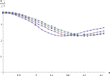
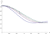
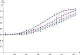
Figure 5.22: Total energy density and the various contributions for $\Omega=1$ varying $\mu$ and $N$. From the left to the right $E$, $V$, $D$.

The specific heat density does not show the peak in zero any more fig.5.23 and the curves does not show any particular point as $N$ increase, actually the peak can be found for higher $\mu$.

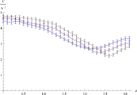
Figure 5.23: Specific heat density for $\Omega=1$ varying $\mu$ and $N$.

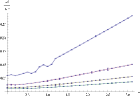
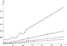
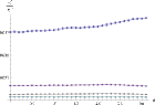
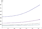
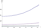
Figure 5.24: Starting from the up left corner and from the left to the right the densities for $\varphi_{a}^{2}$, $\varphi^{2}_{0}$, $\varphi^{2}_{1}$, $Z_{0a}^{2}$, $Z_{00}^{2}$ and $Z_{01}^{2}$ for $\Omega=1$ varying $\mu$ and $N$.

At last in fig.5.24 we found a behavior of the order parameters density for $Z_{0}$ and $\psi$ fields similar to the former graphs for $\Omega=0.5$ and they are compatible with a dilatation of the previous diagrams.

5.2 Two dimensional case

The main aim of this chapter was to show the numerical result for the 4-dimensional model, beside it is very interesting to analyze the 2-dimensional model (which was used as a first test of the program) described by the discretized action (4.44) and note the differences with the full model. Will be used the same set of parameters used for the full model and due to the same dependence on $\alpha$ all the simulation will be conducted with $\alpha=0$.

5.2.1 Varying $\Omega$

The behavior of the energy density for $\mu=\{1,0\}$ is the same of the full model, in the graphs fig 5.25 are plotted the total energy density and the comparison of the various contributions for $\mu=\{1,0\}$. As we can see there is no evident difference from the 4-dimensional case; even in this case the total energy for $\mu=1$ follows the slope of the $D$ contribution and the total energy for $\mu=0$ is constant. Even the various contributions have the same trend of the full model; for $\mu=1$ the $V$ and $F$ have an “opposite“ slope and for $\mu=0$ they balance each other in order to obtain a constant sum.

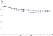
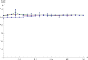
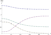
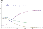
Figure 5.25: Total energy density and contributions for $\mu=1$ (left side) and $\mu=0$ (right side) varying $\Omega$ and $N$. Where $E$ (blue), $V$ (purple), $D$ (brown), $F$ (green).

The specific heat density shows fig.5.26 some differences: for $\mu=0$ the peak is no more located around $\Omega=1$ but it appears, not so clearly, around zero and the specific heat for $\mu=0$ does not show any particular point.

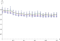
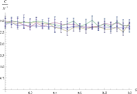
Figure 5.26: Specific heat densities for $\mu=1$ (left) and $\mu=0$ (right) varying $\Omega$ and $N$.

In the figure fig.5.27 are showed the graphs for $\varphi_{a}^{2}$, $\varphi^{2}_{0}$ and $\varphi^{2}_{1}$ and $Z_{0a}^{2}$, $Z_{00}^{2}$ and $Z_{01}^{2}$ for $\mu=1$. For brevity are showed the graphs only for $Z_{0}$, however even for the 2-dim model taking in account the statistical errors they are compatible with the $Z_{1}$ field related graphs.

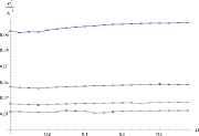
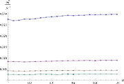
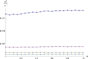
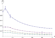
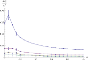
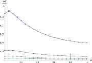
Figure 5.27: Starting from the up left corner and from the left to the right the densities for $\varphi_{a}^{2}$, $\varphi^{2}_{0}$, $\varphi^{2}_{1}$, $Z_{0a}^{2}$, $Z_{00}^{2}$ and $Z_{01}^{2}$ for $\mu=0.5$ varying $\Omega$ and $N$.

In this results there are no significant changes with the 4-dim model, indeed comparing the three graphs fig.5.27 it easy to see the dominance of the spherical contribution $\varphi^{2}_{0}$ to the full power of the field and for the $Z_{0}$ fields the spherical contribution becomes dominant approaching to $\Omega=0$ starting from a zone in which the contributions of $Z_{00}^{2}$ and $Z_{01}^{2}$ are comparable. Beside, we notice a decrease of values of the quantiles related to $\psi$ with $N$, nevertheless the dominance of the $\varphi_{0}$ on the total power of the field remains independently by $N$. The peak appearing in $Z_{0a}^{2}$ and $Z_{00}^{2}$ decrease, but if look at the single graph for fixed $N$ the spherical contribution approaching the point $\Omega=0$ still dominant. The graphs of the previous quantities for $\mu=0$ show the same slope as the full model so will be not presented here.

A radical change emerges for the case $\mu=3$ as in the full model, but the plots of the energy density are very different fig.5.28. From the comparison of the various contributions with the total energy density for $N=20$, we deduce that the total energy density seems to follow the $D$ contribution instead $F$ as in the 4-dim model. This can be justified by the presence of additional terms in the full model coming from the Y-M part.

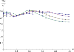
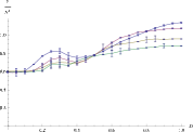
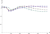
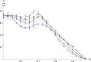
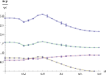
Figure 5.28: Total energy density and contributions for $\mu=1$ varying $\Omega$ and $N$. From the left to the right $E$, $V$, $D$, $F$ and comparison.

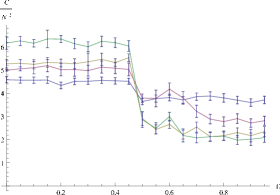
Figure 5.29: Specific heat density for $\mu=3$ varying $\Omega$ and $N$.

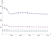
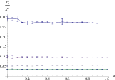
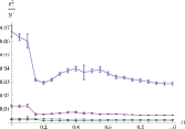
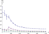
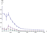
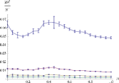
Figure 5.30: Starting from the up left corner and from the left to the right the densities for $\varphi_{a}^{2}$, $\varphi^{2}_{0}$, $\varphi^{2}_{1}$, $Z_{0a}^{2}$, $Z_{00}^{2}$ and $Z_{01}^{2}$ for $\mu=3$ varying $\Omega$ and $N$.

In this case the specific heat density does not shows fig.5.29 the peak for $\Omega=1$, but we discover a step around $\mu\approx 0.5$ this seems to becomes sharper as $N$ increase. Regarding the order parameters $\varphi_{a}^{2}$, $\varphi^{2}_{0}$, $\varphi^{2}_{1}$ and $Z_{0a}^{2}$ $Z_{00}^{2}$, $Z_{01}^{2}$ they have similar behavior of the full model with some more evident oscillations around the origin.

5.2.2 Varying $\mu$

The resemblance between the two models is more evident when we compare the plots obtained fixing $\Omega=\{0,0.5,1\}$ and varying $\mu$. The graphs in fig.5.31 show the total energy density and the various contributions for $\Omega=\{0,0.5,1\}$. It is very clear the similarity with the full model; for $\Omega=0$ appears a peak in the total energy density around $\mu\approx 2.3$ for $N=20$, for $\Omega=0.5$ and $\Omega=1$ the peaks are shifted. The various contributions follows the same behavior of the full model where, in the case $\Omega=1$, the $F$ component is absent due to the vanishing of the prefactor in front of the Y-M part of the action.

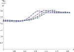
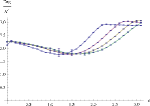
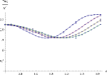
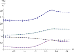
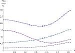
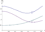
Figure 5.31: Total energy density and contributions for $\mu=1,\alpha=0$ varying $\Omega$ and $N$. From the left to the right $E$, $V$, $D$, $F$ and comparison with $N=5$ (blue), $N=10$ (purple), $N=15$ (brown), $N=20$ (green).

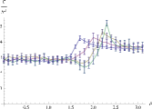
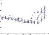
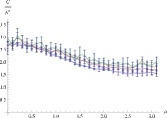
Figure 5.32: Specific heat density for $\Omega=0$ (left) and $\Omega=0.5$ (center), $\Omega=1$ (right) varying $\mu$ and $N$.

The resemblance persists in the specific heat density too, in fig.5.32 the peaks are located as the 4-dim model and for $\Omega=1$ does not appear any peak.

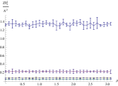
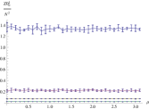
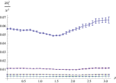
Figure 5.33: From the left to the right the densities for $Z_{0a}^{2}$, $Z_{00}^{2}$ and $Z_{01}^{2}$ for $\Omega=0$ varying $\mu$ and $N$.

At last in fig.5.33 is displayed the behavior of the order parameters density of $Z_{0}$ for $\Omega=0$, even in the 2-dimensional case the slopes of $Z_{0a}^{2}$, $Z_{00}^{2}$ densities are constant within the errors bars. The other orders parameters are identical to the full model related graphs and are compatible with a dilatation of the previous diagrams for $\Omega=0.5$.

Conclusions and prospectives

In this thesis we have presented a study of a spectral action model constructed in order to extend to the Yang-Mills theories the non-commutative Wulkenhaar-Grosse model. The main aim of this work was to test a first Monte Carlo approach based on a non-perturbative regularization method alternative to the standard lattice regularization, which in our case is not suitable due to the oscillator factor of the Moyal product. We have performed Monte Carlo simulations and obtained the values of the defined observables varying the parameters of the system. Despite the complexity of the approximated spectral action considered here we were able to obtain some reliable numerical results, we can conclude that a numerical approach of this kind of model using the matrix Moyal base seems feasible. The specific heat density shows various peaks indicating phase transitions, in particular studying the behaviors for some fixed $\mu$ we found a peak around $\Omega=0$ for $\mu=\{0,1\}$ and peak in $\Omega=1$ for $\mu=3$, beside we notice a huge change in the energy density and in its contributions between the cases $\mu=\{0,1\}$ and $\mu=3$. Others peaks in the specific heat density can be found varying $\mu$ and fixing $\Omega$, the graphs show that increasing $\Omega$ the peak in the specific heat, starting from $\mu\approx 2.4$ for $\Omega=0$, is moved towards higher $\mu$. The order parameters introduced show a strong dependence on the occurrence of $\Omega=0$ or $\Omega\neq 0$. Referring to the fixed $\mu$ graphs we found a peak in the spherical contribution for the gauge fields $Z_{i}$, we can interpreted this slope as a sort of symmetry breaking introduced by $\Omega\neq 0$. Additionally, varying $\mu$ and fixing $\Omega$ the other parameters display an increasing slope with $\mu$ for all fields and all situation but one; the graphs of the order parameters concerning $Z_{0a}$, $Z_{00}$ for $\Omega=0$ show a constant behavior. As an aside result we have ran the same computations on the simpler 2-dimensional model, from the comparison despite many similarities in the results varying $\mu$, we note a complete different trend of the specific heat varying $\Omega$, the peaks present in the full model does not appear any more in the 2-dimensions one. From this comparison we deduce that the dimension is a crucial parameter of the model. About the prospective, there is a lot of work to do; the natural next steps in the numerical study of this model, could be the computation of the transition curves in order to separate the phase regions and classify them using eventually some additional order parameters. Our treatment, forced by limited resource, was conducted conjecturing that the system can fully described varying $\Omega$ in the range $[0,1]$ but since the L-S duality does not hold any more in our case, will be very useful to extend this range. Actually, the computed graphs does not show any periodicity in $\Omega\in[0,1]$ so there are some hints to infer that the range $[0,1]$ is not enough, however only a direct computation will clarify this point. At last, in analogy with the matrix model will be very interesting to do not require any more the condition $\mu^{2}>0$, in order to implement this change we have to conduct the calculation no more around the minimum of the actions. The problems that can occur are related the thermalization process, which can be much more problematic due to the eventual emerging of local minimum. The expansion of the parameters space, together with the classification of the different phase regions allows us to compare our model with the results of the simulation conducted on the fuzzy spaces, looking in particular about the occurrence of the so called non-uniformly ordered phase which is connected with the UV/IR mixing. Since we have constructed our model starting from a renormalizable one this study is very desirable.

Appendix A Axioms non-compact geometries

In this appendix will be introduced the definition of non-compact spectral triple and the modified set of axioms required for such spectral triple. In the last part of the chapter will be hinted a more rigorous treatment of the spectral triple used in chapter 3, extending it in the setting of non-compact triple.

A.1 General remarks

A compact spectral triple is a collection $(\mathcal{A},\mathcal{D},\mathcal{H})$ where $\mathcal{A}$ is a unital pre-$C^{*}$-algebra, $\mathcal{H}$ is a Hilbert space on which $\mathcal{A}$ is represented by bounded operators and $\mathcal{D}$ is a Dirac selfadjoint operator on $\mathcal{A}$, with resolvent $R_{\mathcal{D}}(\lambda)=(\mathcal{D}-\lambda)^{-1}$ compact and the commutator $[\mathcal{D},a]$ is bounded on $\mathcal{H}$ for every $a\in\mathcal{A}$. In the non-compact case this definition is modified to allow $\mathcal{A}$ to be no longer unital. The usual way to construct a non-commutative spin manifolds, for the unital case, is to start from an operatorial version of ordinary spin geometry that can be generalized to a non-commutative manifold. This generalization is obtained using a reconstruction theorem in order to recover all of the structure from the abstract geometry over a suitable algebra [28, 35, 68]. However, there is no proper direct reconstruction theorem for non-compact Riemanian spin manifolds, so the question of axioms for non-unital spectral triples is guided by the resemblance to the compact case, requiring a collection of axioms for not necessarily compact non-commutative manifolds. Of course, such list of conditions should be compatible with the previous axiomatic framework and be fulfilled by non-compact commutative manifolds. Modified systems of axioms for non-compact spectral triples has been formulated by A. Rennie [69] for the commutative case and by Gayral et al. [55] in a fully non-commutative framework on the Moyal plane. A very important aspect for these formulations is the introduction of various different types of non-commutative dimension [70]. Indeed, the non-compact spectral triple analyzed will be characterized by different metric and KO-dimensions. When $\mathcal{A}$ is not unital, we need to choose a preferred unitization $\mathcal{B}$. For compact or unital spectral triples it is further required that the operator $\mathcal{D}$ has a compact resolvent, or in other words, $(\mathcal{D}-\lambda)^{-1}$ must belong to $K(\mathcal{H})$ for $\lambda\notin sp\mathcal{\mathcal{D}}$, where $K(\mathcal{H})$ denote the compact operators on $\mathcal{H}$. Consequently $\mathcal{D}$ must have discrete spectrum of finite multiplicity. Since this is clearly not the case of Dirac operator ${\not}\mathcal{D}$ on $\mathbb{R}^{d}$, in the nonunital case we only demand [35] that $a(\mathcal{D}-\lambda)^{-1}$ is compact for $a\in\mathcal{A}$. This condition ensures that the spectral triple $(\mathcal{A},\mathcal{D},\mathcal{H})$ corresponds to a well-defined $d$-homology class [73] for an, in general, non-compact non-commutative geometry. Now we analyze some modified conditions which spectral triples are required to satisfy. We use a regularity condition [57] in terms of the operator $\langle\mathcal{D}\rangle=(\mathcal{D}^{2}+1)^{\frac{1}{2}}$, in this way we avoid the hypothetical zero modes of the Dirac operator. Can be shown that the previous regularity condition coincides with the original definition of Connes and Moscovici [39]. The condition of finiteness, in the unital case, is that the smooth domain $\mathcal{H}^{\infty}$ of $\mathcal{D}$ in $\mathcal{H}$ can be finitely generated by a projective left module over the unital algebra $\mathcal{A}$, or $\mathcal{H}^{\infty}\sim\mathcal{A}^{m}p$ for some projector $p$ in $M_{m}(\mathcal{A})$ with a suitable $m$. In the case of $\mathbb{R}^{d}$, using the commutative or the Moyal product, the module of smooth spinors is free, since the triviality of the spinor bundle.

When $\mathcal{A}$ is nonunital, in order to obtain a projective $\mathcal{A}$-module, we have to find the projector $p$ in a matrix algebra over the preferred compactification $\mathcal{B}$, therefore this condition for the nonunital case should then require that $\mathcal{H}^{\infty}$ densely contains a pullback of a finite projective $\mathcal{B}$-module to $\mathcal{A}$. The reality axiom is the same as the compact case, thus is the existence of an antilinear conjugation operator $J$ on $\mathcal{H}$ such that a $\to Ja^{*}J^{-1}$, which define an another representation of $\mathcal{A}$ on $\mathcal{H}$ commuting with the previous one. The required algebraic properties of the real structure $J$ are the same as the compact case. Even for the first order condition, there is no need to modify the axiom in the non-compact case, we have:

$$[[\mathcal{D},a],Jb^{*}J^{-1}]=0,\ \textrm{for all}\ a,b\in\mathcal{A}.$$ (A.1)

It is convenient formulate the orientability condition in the compact case as the property that the spectral triple $(\mathcal{A},\mathcal{H},\mathcal{D})$ contains an algebraic version of a volume $d$-form. This algebraic version consists of an Hochschild $d$-cycle $c$, which is a sum of terms of the form $(a_{0}\otimes b^{o}_{0})\otimes a_{1}\otimes\cdots\otimes a_{d}$ satisfying the cycle property $bc=0$. Defining $b_{0}^{o}$ as an element of the opposite algebra $\mathcal{A}^{o}$ with $b_{0}\in\mathcal{A}$, we can represent the Hochschild $d$-cycle by bounded operators:

$$\pi_{\mathcal{D}}((a_{0}\otimes b^{o}_{0})\otimes a_{1}\otimes\cdots\otimes a_{d})=a_{0}Jb^{*}_{0}J^{-1}[\mathcal{D},a_{1}]\cdots[\mathcal{D},a_{d}].$$ (A.2)

on which we impose the orientation $\pi_{\mathcal{D}}(c)=\chi$, where $\chi$ is the given $\mathbb{Z}_{2}$-grading operator on $\mathcal{H}$. We just use $\chi=1$ if $d$ is odd and in the even case, for ordinary spinors, we use

$$\chi=(-i)^{m}\gamma^{1}\gamma^{2}\cdots\gamma^{2m}$$ (A.3)

For nonunital algebras, we ask the same condition taking the cycle over the unitization $\mathcal{B}$ rather than $\mathcal{A}$ itself.

A.2 Modified conditions for nonunital spectral triples

By a real non-compact spectral triple of dimension $k$ we connote the data
$(\mathcal{A},\mathcal{B},\mathcal{H},\mathcal{D},J,\chi),$ where $\mathcal{A}$ is an algebra, in general nonunital, acting faithfully via a representation denoted by $\pi$ on the Hilbert space $\mathcal{H}$, $\mathcal{B}$ is a preferred unitization of $\mathcal{A}$ acting on the same Hilbert space and $\mathcal{D}$ is an unbounded selfadjoint operator on $\mathcal{H}$ such that $[\mathcal{D},a]$ for each $a$ in $\mathcal{B}$ extends to a bounded operator on $\mathcal{H}$. In addition, $J$ and $\chi$ are respectively an antiunitary and a selfadjoint operator, such that $\chi=1$ when $k$ is odd and otherwise $\chi^{2}=1$, $\chi a=a\chi$ for $a\in\mathcal{A}$ and $\mathcal{D}\chi=-\chi\mathcal{D}$. This objects are asked to satisfy the conditions below.

0.Regularity

The bounded operator , $\pi(a)$ and $[\mathcal{D},\pi(a)]$ for all $a\in\mathcal{B}$ belongs to $\bigcap_{n=1}^{\infty}\textrm{Dom}(\delta^{n})$, with $\delta(T)=[\langle\mathcal{D}\rangle,T]$ and $\langle\mathcal{D}\rangle=(\mathcal{D}^{2}+1)^{\frac{1}{2}}$

1.Compactness

The operator $\pi(a)(\mathcal{D}-\lambda)^{-1}$ is compact for all $a\in\mathcal{A}$ and $\lambda\in sp(\mathcal{D})$, where $sp(\mathcal{D})$ is the spectrum of $\mathcal{\mathcal{D}}$.

2.Spectral dimension

For any element $b$ of the algebra $\Psi_{0}(\mathcal{A})$ generated by $\delta^{n}(\pi(\mathcal{A}))$ and $\delta^{n}([D,\pi(\mathcal{A})])$, the function $\zeta_{b}(z)=\textrm{Tr}(b\langle\mathcal{D}\rangle^{-z})$ is well defined, holomorphic for $\mathfrak{R}(z)$ large and analytically continues to $\mathbb{C}/\textrm{Sd}$, where $\textrm{Sd}\subset\mathbb{C}$ is a discrete set called dimension spectrum. The dimension spectrum is said simple if all the poles are simple, finite if there is a $k\in\mathbb{N}$ such that all the poles are of the order at most $k$ and if it is finite.

3. Metric dimension

The metric dimension is defined as $d=sup\{\mathfrak{R}(z),z\in\textrm{Sd}\}$, the operator $\pi(a)\langle\mathcal{D}\rangle^{-d}$ belongs to the Dixmier class $\mathcal{L}^{1}_{\omega}(\mathcal{H})$ for any $a\in\mathcal{A}$. For any Dixmier trace the map $a\in\mathcal{A}_{+}\to Tr_{\omega}(\pi(a)\langle\mathcal{D}\rangle^{-d})$ in non vanishing.

4.Finiteness

The algebra $\mathcal{A}$ and its preferred unitization $\mathcal{B}$ are pre-$C^{*}$-algebras. Each one is a $\star$-subalgebra of some $C^{*}$-algebra, stable under holomorphic functional calculus. The space of smooth spinors

$$\mathcal{H}^{\infty}=\bigcap_{n=0}^{\infty}\mathcal{H}^{n},\ \textrm{where}\ \mathcal{H}^{n}=\textrm{Dom}(\mathcal{D}^{n})$$ (A.4)

completed with the norm $||\xi||^{n}=||\xi||^{2}+||\mathcal{D}^{n}\xi||^{2}$, is a finitely generated projective $\mathcal{A}$-module $p\mathcal{A}^{m}$ for some $m\in\mathbb{N}$ and some projector $p=p^{2}=p^{*}\in M_{m}(\mathcal{B})$. The scalar product $(\cdot,\cdot)$ on $\mathcal{H}^{\infty}$ can be obtained composing the Dixmier trace and the induced structure $\langle\cdot,\cdot\rangle:\mathcal{H}^{\infty}\times\mathcal{H}^{\infty}\to\mathcal{A}$

$$\textrm{Tr}_{\omega}(\langle\xi,\eta\rangle\langle\mathcal{D}\rangle^{-d})=(\xi,\eta),\ \xi,\eta\in\mathcal{H}^{\infty}$$ (A.5)

5.Reality

There is an antiunitary operator $J$ on $\mathcal{H}$, such that:

$$[\pi(a),J\pi(b^{*})J^{-1}]=0,\ \textrm{for all}\ a,b\in\mathcal{B}$$ (A.6)

$b\to Jb^{*}J^{-1}$ is a commuting representation on $\mathcal{H}$ of the opposite algebra $\mathcal{A}^{o}$. Beside, the operator is required to satisfy $J=\epsilon$ and $J\mathcal{D}=\epsilon^{\prime}\mathcal{D}J$ and also for the even case $J\chi=\epsilon^{\prime\prime}\chi J$ , where $\epsilon,\epsilon^{\prime},\epsilon^{\prime\prime}\in\{-1,1\}$ given as a function of $k_{O}\in\mathbb{Z}_{8}$. This function is represented by the table:

$$\begin{array}[]{|c|c|c|c|c|c|c|c|c|}\hline\cr k_{O}\ \textrm{mod 8}&0&1&2&3&4&5&6&7\\ \hline\cr\epsilon&1&1&-1&-1&-1&-1&1&1\\ \hline\cr\epsilon^{\prime}&1&-1&1&1&1&-1&1&1\\ \hline\cr\epsilon^{\prime\prime}&1&&-1&&1&&-1&\\ \hline\cr\end{array}$$ (A.7)

This $k_{O}$ is usually referred as the KO dimension of the spectral triple.

6.First order

The bounded operators $[\mathcal{D},\pi(a)]$ also commute with the opposite algebra representation:

$$[[\mathcal{D},\pi(a)],J\pi(b^{*})J^{-1}]=0,\ \textrm{for all}\ a,b\in\mathcal{B}.$$ (A.8)

7.Orientation

There is an Hochschild $d$-cycle $c$ on $\mathcal{B}$, with values in $\mathcal{B}\otimes\mathcal{B}^{\prime o}$. Such $d$-cycle is a finite sum of terms like $(a\otimes b^{o})\otimes a_{1}\otimes\cdots\otimes a_{k}$, which can be naturally represented by operators on $\mathcal{H}$ using $\pi_{\mathcal{D}}(c)$ in formula (A.1). The volume form $\pi_{\mathcal{D}}(c)$ must solve the equations:

$$\pi_{\mathcal{D}}(c) = \chi\ \textrm{even case}$$ (A.9)

$$\pi_{\mathcal{D}}(c) = 1\ \textrm{odd case}$$ (A.10)

A geometry is called connected or irreducible if the only operators commuting with $\mathcal{A}$ and $\mathcal{D}$ are the scalars.

Poincaré duality, for a non-compact orientable manifold $M$, is usually expressed as the isomorphism between the compactly supported de Rham cohomology and the homology of $M$ mediated by the fundamental class [M]. We shall actually leave aside the final condition of Poincaré duality, since it is not central in the present work.

A.3 Non-compact harmonic Moyal case

Referring to the spectral triple $(\mathcal{A}_{4},\mathcal{D}_{4},\mathcal{H}_{4})$ defined in the chapter 3 it is possible to extend the previous triple to a non-compact spectral triple of metric dimension 4 and KO dimension 0. In this section will be just listed the theorems about compactness, boundness, regularity and dimension remanding to [57] for the complete proofs.

Compactness and Boundness

As first step we define a preferred unitisation $\mathcal{B}_{4}$ of $\mathcal{A}_{4}$ as the space of smooth bounded function on $\mathbb{R}^{4}$ with all partial derivatives bounded. The Moyal product extend to $\mathcal{B}_{4}$ and $\mathcal{A}_{4}\subset\mathcal{B}_{4}$ is not a dense two-side essential ideal [55]. The algebra $\mathcal{B}_{4}$ contains the plane waves $e^{ikx}$ and constant functions but no other non-constant polynomials. Can be proved [55] that $\mathcal{B}_{4}$ is contained in the $C^{*}$-algebra:

$$A_{4}=\{T\in S^{\prime}(\mathbb{R}^{4})\ :\ T\star f\in L^{2}(\mathbb{R}^{4})\ \textrm{for all}\ f\in L^{2}(\mathbb{R}^{4})\}$$ (A.11)

completed using operator norm. Defining the action $\pi=L_{\star}$ of $\mathcal{B}_{4}$ on $\mathcal{H}_{4}$ as the componentwise left star multiplication:

$$\star:\mathcal{A}_{4}\times\mathcal{H}_{4}\to\mathcal{H}_{4},\ \ (f,\psi)\to L_{\star}(f)\psi=f\star\psi$$ (A.12)

For $f\in\mathcal{B}_{4}$ the operator $\pi(f)$ is bounded. The commutator $[\mathcal{D}_{4},\pi(f)]$ is computed using the relation (2.25)

$$\mathcal{D}_{4}(f\star\psi)-f\star(\mathcal{D}_{4}\psi)=(i(\Gamma^{\mu}+\Omega\Gamma^{\mu+4})(\partial_{\mu}f))\star\psi$$ (A.13)

with $f\in B_{4}$ and $\psi\in\textrm{Dom}(\mathcal{D}_{4})\bigcap\textrm{Dom}(\mathcal{D}_{4})\pi(f)$. We deduce that for $\partial_{\mu}f\in\mathcal{B}_{4}$ the commutator is extended to a bounded operator. The compactness is verified taking in account that $(\mathcal{D}_{4}^{2}+1)^{-1}$ is already a compact operator on $\mathcal{H}_{4}$, as bounded operator $K$ is compact if and only if $KK^{*}$ is compact too. In particular, we have that the operator $(\mathcal{D}_{4}+i)^{-1}$ is compact, beside the definition resolvent equation implies that $(\mathcal{D}_{4}+\lambda)^{-1}$ is compact for any $\lambda$ in the resolvent set of $\mathcal{D}_{4}$. Whence $\pi(f)(\mathcal{D}_{4}+\lambda)^{-1}$ is compact for $f\in\mathcal{B}_{4}$.

Regularity and dimension

As in the compact case it is useful for the non-compact too, to define the unbounded operators $R$ and $L$ as

$$R(T)=[\mathcal{D}_{4}^{2},T]\langle\mathcal{D}_{4}\rangle^{-1},\ L(T)=\langle\mathcal{D}_{4}\rangle^{-1}[\mathcal{D}_{4}^{2},T]$$ (A.14)

Can be proved that they satisfy $\bigcap_{n=1}^{\infty}\textrm{Dom}\delta^{n}=\bigcap_{m,n=1}^{\infty}\textrm{Dom}R^{n}L^{m}$. Using this derivation can be demonstrated [57] the following proposition:

Proposition 1.

Both $\pi(f)$ and $[\mathcal{D}_{4},\pi(f)]$ belong for any $f\in\mathcal{B}_{4}$ to $\bigcap_{n=1}^{\infty}\textrm{Dom}\delta^{n}$, where $\delta^{n}$ are defined by the axiom 0.

For the dimension spectrum we have the following theorem:

Theorem 1.

The spectral triple $(\mathcal{A}_{4},\mathcal{D}_{4},\mathcal{H}_{4})$ has dimension spectrum Sd$=4-N$ and therefore metric dimension 4.

Appendix B Error estimation and update algorithm

In this appendix will be introduced the treatment of the statistical error in Monte Carlo simulation and will be discussed three methods to estimate the statistical errors. In the end of the section will be discussed some issues concerning the estimation of the autocorrelation time and the implemented update algorithm.

We start defining the mean $O$ over a subset of $\{O_{i}\}^{T_{MC}}_{i=1}$ of $T$ elements as a simple arithmetic mean over the Markov chain:

$$\bar{O}=\frac{1}{T}\sum_{i=1}^{T}O_{i}$$ (B.1)

where $T_{MC}$ are total number of measurements of the time series. The expectation value of $O$ is an ordinary number, meanwhile the estimator $\bar{O}$ is a random number fluctuating around the theoretically expected value. For numerical simulations the estimation would require to repeat the simulation several times, forced by the limit of computing power, the fluctuations of the mean value are not probed directly. The usual way is to estimates its variance:

$$\sigma^{2}_{\bar{O}}=\langle(\bar{O}-\langle\bar{O}\rangle)^{2}\rangle=\langle\bar{O}^{2}\rangle-\langle\bar{O}\rangle^{2}$$ (B.2)

using the distribution of the individual measurements of $O$. In case of uncorrelated subsequent $T_{MC}$ measurements the previous formula reduces to:

$$\sigma^{2}_{\bar{O}}=\frac{\sigma^{2}_{O}}{T_{MC}}$$ (B.3)

$\sigma^{2}_{O}$ is the variance of the individual measurements. Explicitly the (B.3) expression is:

$$\sigma_{\bar{O}}=\sqrt{\frac{\frac{1}{T}\Sigma_{i=1}^{T}(O_{i}-\bar{O})}{T-1}}=\sqrt{\frac{1}{T-1}\left(\overline{O^{2}}-(\bar{O})^{2}\right)}$$ (B.4)

To formulate the (B.2) we assume time-translation invariance over the Markov chain and the equilibrium of simulation (values taken after the thermalization) for any distribution $P(O)$ of the $O$. It is usual to refer to $\sigma_{\bar{O}}$ as the variance of the mean, it is the squared width of this distribution and is used as the squared error quoted together with the value $\bar{O}$. In the case of a Gaussian distribution we have a probability of about 68% that all identical simulations will produce a mean value in the interval $[\bar{O}-\sigma_{\bar{O}},\bar{O}+\sigma_{\bar{O}}]$. If we use $2\sigma$ as the error the percentage become about 95% and for $3\sigma$ interval the probability is higher than 99.7%.

If the samples are not statistically independent (B.3) becomes an under-estimation of the error. The correct expression for $\sigma_{\bar{O}}$ is [77]:

$$\sigma_{\bar{O}}=\sqrt{\frac{1+\frac{2\tau}{\Delta T}}{T-1}\left(\overline{O^{2}}-(\bar{O})^{2}\right)}$$ (B.5)

where $\Delta T$ is the Monte Carlo time interval ($T=T_{MC}/\Delta T$) and $\tau$ is called autocorrelation time. The autocorrelation time is defined as [79]:

$$\tau=\frac{1}{2}+\sum_{k=1}^{T}A(k)\left(1-\frac{k}{T}\right)$$ (B.6)

with

$$A(k)=\sum_{i=1}^{i+k\leq T}\frac{\langle O_{i}O_{i+k}\rangle-\langle O_{i}\rangle\langle O_{i}\rangle}{\langle O_{i}\rangle-\langle O_{i}\rangle\langle O_{i}\rangle}$$ (B.7)

For large $T$ and $2\tau$, equation (B.5) turns into:

$$\sigma_{\bar{O}}=\sqrt{\frac{2\tau}{T_{MC}}\left(\overline{O^{2}}-(\bar{O})^{2}\right)}$$ (B.8)

The equation (B.5) states that due to temporal correlations of the measurements the real statistical error $\sigma_{\bar{O}}$ of the Monte Carlo estimator $\bar{O}$ is multiplied by a factor of $\sqrt{2\tau}$. We can reformulate the correlated statistical error looking to the uncorrelated case as:

$$\sigma^{\prime}_{\bar{O}}=\sqrt{\frac{\sigma^{2}_{O}}{T_{eff}}}$$ (B.9)

but now with a effective statistic parameter

$$T_{eff}=\frac{T_{MC}}{2\tau}\leq T_{MC}$$ (B.10)

The effective statistic, for correlated data, is smaller of the number total number of measurements and are approximately uncorrelated for $2\tau$ iterations. To obtain an acceptable error estimation (especially for such quantity like specific heat and susceptibility) a simulation has to provide an estimation of autocorrelation times too.

B.1 Methods to estimate the error

B.1.1 Binning method

In many cases the absence of autocorrelations time factor on statistical errors bring an great underestimation, beside the calculus of autocorrelation time usually involves a big amount of computation time. The statistical error underestimation can occur even for completely uncorrelated data in time, in fact arises the problem of the error estimation for quantities that are not directly measured in the simulation but are derived as a general combination of direct measures, but in this case can be use the error propagation. An good balance, in some situation, can be found using some alternative methods to estimate the statistical errors; the binning analysis is much more easy to compute but is less accurate of the direct computation. This method consist to split the original correlated measurements vector $\{O_{i}\}^{T_{MC}}_{i=1}$ into smaller non-overlapping $T_{B}$ blocks of length $k$ such that $T_{MC}=T_{B}k$ and compute the block average $O_{B,n}$ of the $n$-th block

$$O_{B,n}=\frac{1}{k}\sum^{k}_{i=1}O_{(n-1)k+i}$$ (B.11)

with $n=1,\cdots,T_{B}$. The mean value over all block satisfies the identity $\bar{O}_{B}=\bar{O}$. For block length $k$ large enough $(k\ll\tau)$ the blocks become approximately uncorrelated, therefore the variance can be computed according to the uncorrelated estimator (B.4). Resuming, we have for the squared statistical error of the mean value:

$$\sigma^{2}_{\bar{O}}=\frac{\sigma^{2}_{B}}{T_{B}}=\frac{1}{T_{B}(T_{B}-1)}\sum^{T_{B}}_{n=1}(O_{B,n}-\bar{O}_{B})^{2}$$ (B.12)

To obtain an acceptable result we must probe various partition of $T_{B}$ and select the one which maximize the statistical error. The main disadvantage of this method is the strongly dependence of the error on the choice of the partition $T_{B}$

B.1.2 Jackknife estimation

This approach [84, 85] is a variation of the binning method and can be viewed as a re-sampling. This method too concerns to separate the vector of measurements into $T_{B}$ blocks but instead consider small blocks of length $k$, in the Jackknife method we build $T_{B}$ large Jackknife blocks $O_{J,n}$ containing all measurements but omitting the data contained in the previous $n$-th binning block:

$$O_{J,n}=\frac{T_{MC}\bar{O}-kO_{B,n}}{T_{MC}-K}$$ (B.13)

with $n=1,\cdots,T_{B}$. The Jackknife blocks consists of $T_{MC}-k$ data, in this way the $n$-th block contains almost every measurements of the complete vector. This allows to use this method even to estimate the errors in non-linear combinations of measured variables, the bias is comparable to that of the total data. This choice of the $T_{B}$ Jackknife blocks makes them trivially correlated due to the common data coming from the same original data in $T_{B}-1$ different Jackknife blocks. However, this correlation is a pure re-sampling and it is not connected to time correlation. As a consequence, it does not magnify the error but the Jackknife block variance $\sigma_{J}$ will be smaller than the variance computed using binning method. This reduction can be corrected by multiplying $\sigma^{2}_{J}$ with a factor $(T_{B}-1)^{2}$, obtaining:

$$\sigma^{2}_{\bar{O}}=\frac{T_{B}-1}{T_{B}}\sum^{T_{B}}_{n=1}(O_{J,n}-\bar{O}_{J})^{2}$$ (B.14)

B.2 Numerical estimation of autocorrelation time

A third option, the so called Sokal-Madras method [83], is an hybrid approach founded on the estimation of the autocorrelation time using (B.6)-(B.7). In the case that the autocorrelation time satisfies $\tau<0.5$ the samples are not correlated thus, to estimate the error, is used the standard uncorrelated error given by (B.4) otherwise error is given by (B.7).

An estimation of the autocorrelation time is important not only for the error estimation, but also for the computation of static quantities themselves. In general, it is very hard to have a priori estimation and a direct numerical analysis is usually too time consuming. An estimator $\hat{A}(k)$ for the autocorrelation function is obtained by replacing in (B.7) the expectation values by mean values. Can be shown that increasing $k$ the variance of $\hat{A}(k)$ grows quickly, to achieve an rough estimation of $\tau$ and thus a correct error estimate, it is useful to record the partial autocorrelation time estimator

$$\tau^{\prime}(k_{max})=\frac{1}{2}+\sum^{k_{max}}_{K=1}\hat{A}(k)$$ (B.15)

In the limit of large $k_{max}$ the previous sum tents to $\tau$, unfortunately its statistical error increases rapidly. An usual procedure, used to find a reasonable balance between systematic and statistical errors, is to determine a self-consistently upper limit $k_{max}$ by cutting off the summation for $k_{max}>6\tau^{\prime}(k_{max})$.

In this thesis were compared the errors obtained using the previous three methods. Referring to the basic observables like energy density $E$ and the order parameters like $\varphi_{i}$, $Z_{i\mu}$, we have found that the errors were compatible among the three methods. For quantities like the specific heat the errors were no more compatible, therefore was applied the more accurate Sokal-Madras method using the described cut for the estimation of the correlation time.

B.3 The update algorithm

The model considered in this works involves five complex independent matrices for the 4-dimensional case and 3 complex independent for the 2-dimensional one, beside the approximated actions are quite complex and contain terms up the fourth power. The usual update algorithm, used to generate a new configuration, expects to change all the entries of the independent matrices:

$$\psi_{ij}\longrightarrow\psi_{ij}+a_{0ij},\ \ Z_{kij}\longrightarrow Z_{kij}+a_{kij},\ \textrm{with}\ k=0,\cdots 4,\ i,j=1,\cdots N$$ (B.16)

where $N$ is the matrix size and $a_{kij}$ are random complex numbers in which the real and imaginary parts vary in $[-2,2]$. The amplitude of the random interval was numerically determined to obtain stable results for the observables for larger interval. The new proposed configurations are judged by the metropolis algorithm, which requires to recompute the action for the new proposed configuration. Using an optimized algorithm, this operation involves for each Metropolis check, about $16N^{3}$ or $6N^{3}$ (taking in account the cross products between the independent matrices present in the actions) as a leading order of number of operations respectively for the 4-dimensional and 2-dimensional case. In order to reduce the computation time, instead update all entries we have changed just one matrix coefficient for each Monte Carlo step, the coefficient to update is not chosen randomly but following an order used to vary all the coefficients after $5N^{2}$ or $3N^{2}$ steps. In this way to execute the Metropolis check we can compute the variation of the action respect the previous configuration with a leading order of operations proportional to $N$. The drawback of this approach are manly two: the complication of the code and the behavior of the correlation time in $N$. In fact two configurations will share at least one coefficient until $5N^{2}$ or $3N^{2}$ Monte Carlo steps, this correlations introduce an increasing of the correlation time increasing $N$ and presumably $\tau$ behaves like $5N^{2},\ 3N^{2}$. However, using this optimization, together with the already showed theoretical simplifications and the implementation of parallel computing, we were able to execute our simulation for $N=20$ with sufficient precision and in reasonable time despite our limited computation resource.

References

- [1] H. Weyl, The theory of Groups and Quantum Mechanics, Dover (1931) translation of Gruppentheorie und Quantemmechanik, Hirzel Verlag(1928).
- [2] E.P. Wigner, On the Quantum Correction For Thermodynamic Equilibrium, Phys. Rev. 40 (1932) 749.
- [3] P.Deligne, P. Etingof, D. S. Freed, L. C. Jeffrey, Quantum Fields and Strings: A Course for Mathematicians Vol.2, American Mathematical Society (1999).
- [4] J. Zinn-Justin, Quantum Field Theory and Critical Phenomena, Oxford University Press, Second edition (1993).
- [5] N. Seiberg and E. Witten, String Theory and Noncommutative Geometry, JHEP 9909 (1999) 032, [hep-th/9908142].
- [6] G. S. Agarwal and E. Wolf, Calculus For Functions Of Noncommuting Operators And General Phase-Space Methods In Quantum Mechanics. Mapping Theorems And Ordering Of Functions Of Non-commuting Operators, Phys. Rev. D 2 (1970) 2161.
- [7] J.C. Varilly, J.M. Gracia-Bondia, On the ultraviolet behaviour of quantum fields over noncommutative manifolds, Int.J.Mod.Phys. A14 (1999) 1305, [hep-th/9804001].
- [8] M. Chaichian, A. Demichev and P. Presnajder, Quantum Field Theory on Noncommutative Space-Times and the Persistence of Ultraviolet Divergences, [hep-th/9812180].
- [9] S. Doplicher, K. Fredenhagen, J.E. Roberts, The Quantum Structure of Space-Time at the Planck Scale and Quantum Fields, Phys.Lett.B331:39-44,(1994).
- [10] M.R. Douglas, D-Geometry and Noncommutative Geometry, [hep-th/9901146].
- [11] C.P. Martin and D. Sanchez-Ruiz, The One-loop UV Divergent Structure of U(1) Yang-Mills Theory on Noncommutative , Phys.Rev.Lett. 83 (1999) 476-479, [hep-th/9903077].
- [12] T. Filk, Divergencies in a field theory on quantum space, Phys.Lett. B376 (1996) 53-58.
- [13] T. Krajewski, R. Wulkenhaar,Perturbative quantum gauge fields on the noncommutative torus, [hep-th/9903187].
- [14] S. Minwalla, M. Van Raamsdonk, N. Seiberg, Noncommutative perturbative dynamics, JHEP 0002 (2000) 020 [arXiv:hep-th/9912072].
- [15] I. Chepelev, R. Roiban,Convergence theorem for non-commutative Feynman graphs and renormalization, JHEP 0103 (2001) 001 [arXiv:hep-th/0008090].
- [16] A. Matusis, L. Susskind and N. Toumbas, The IR/UV connection in the non-commutative gauge theories, JHEP 0012 (2000) 002 [arXiv:hep-th/0002075].
- [17] E. Langmann and R. J. Szabo, Duality in scalar field theory on noncommutative phase spaces, Phys. Lett. B533 (2002) 168–177, [hep-th/0202039].
- [18] V. Rivasseau, F. Vignes-Tourneret, R. Wulkenhaar, Renormalization of non-commutative -theory by multi-scale analysis, Phys. Lett. B533 (2002) 168–177, [hep-th/0202039].
- [19] V. Rivasseau, Constructive Matrix Theory, arXiv:0706.1224 [hep-th].
- [20] V. Rivasseau, F. Vignes-Tourneret and R. Wulkenhaar, Renormalization of noncommutative -theory by multi-scale analysis, Commun. Math. Phys. 262 (2006) 565 [arXiv:hep-th/0501036].
- [21] R. Gurau and V. Rivasseau, Parametric representation of noncommutative field theory,Commun. Math. Phys. 272 (2007) 811 [arXiv:math-ph/0606030].
- [22] J. Magnen and V. Rivasseau, Constructive field theory without tears, arXiv:0706.2457[math-ph].
- [23] J. Madore, S. Schraml, P. Schupp, J. Wess, Gauge theory on noncommutative spaces, Eur. Phys. J. C 16 (2000) 161 [arXiv:hep-th/0001203].
- [24] J. Madore, An Introduction to Noncommutative Differential Geometry and its Physical Applications, Cambridge University Press (1995).
- [25] J. C. T. Pool, Mathematical Aspects of the Weyl Correspondence, Phys. 7 (1), 66-76 (1996).
- [26] H. Grönewold, On principles of quantum mechanics, Physica 12, (1946) 405.
- [27] J.M. Gracia-Bondia, Generalized Moyal quantization on Homogeneous Aymplectic Spaces, Contemporary Mathematics, 134 (1992) 93.
- [28] J.M. Gracia-Bondia, J.C. Varilly, H. Figueroa, Elements of noncommutative geometry,Birkhäuser Advanced Texts, Birkhäuser, Boston, (2001).
- [29] J.M. Gracia-Bondia, J.C. Varilly, H. Figueroa, Algebras of distributions suitable for phase-space quantum mechanics, I, J. Math. Phys. 29, (1988).
- [30] K. Gottfried, Quantum mechanics Vol. I: FundamentalsBenjamin, New York (1966).
- [31] A. Connes, Noncommutative Geometry, Academic Press, Inc. (1994).
- [32] A. Connes, Geometry from the spectral point of view, Lett. Math. Phys. 34 (1995), no. 3, 203–238.
- [33] A. Connes, On the spectral characterization of manifolds, (2008) arXiv:0810.2088v1[math.OA].
- [34] A. Connes, Essay on Physics and Non-commutative Geometry, The Interface of Mathematics and Particle Physics, ed. D.G.Quillen et al. Clarendon press, Oxford, (1990).
- [35] A. Connes, Noncommutative geometry and reality, J. Math. Phys. 36 (1995) 6194.
- [36] A. Connes, Gravity coupled with matter and the foundation of noncommutative geometry, Comm. Math. Phys. 155 (1996) 109.
- [37] A. Connes and J. Lott, Particle models and noncommutative geometry (expanded version), Nucl. Phys. Proc. Suppl. 18B (1991) 29.
- [38] A. Connes and J. Lott, Particle Models and Noncommutative Geometry, Nucl.Phys.B (Proc.Suppl.)18B (1990) 29-47.
- [39] A. Connes, H. Moscovici, The local index formula in noncommutative geometry, GAFA 5 (1995) 174–243.
- [40] H. Chamseddine and A. Connes, The Spectral Action Principle, Math.Phys.186:731-750 (1997).
- [41] H. Chamseddine, Alain Connes, Matilde Marcolli, Gravity and the standard model with neutrino mixing, Adv.Theor.Math.Phys.11:991-1089, (2007) [arXiv:hep-th/0610241v1].
- [42] F. Lizzi, G. Mangano, G. Miele, and G. Sparano, Fermion Hilbert space and fermion doubling in the noncommutative geometry approach to gauge theories, Phys. Rev. D55:6357–6366, (1997).
- [43] H. Grosse and R. Wulkenhaar, Power-counting theorem for non-local matrix models and renormalisation, [arXiv:hep-th/0305066].
- [44] H. Grosse and R. Wulkenhaar, Renormalisation of -theory on noncommutative in the matrix base, Commun. Math. Phys. 256 (2005) 305 [arXiv:hep-th/0401128].
- [45] H. Grosse and R. Wulkenhaar, -spectral triple on -Moyal space and the vacuum of noncommutative gauge theory, arXiv:0709.0095[hep-ht].
- [46] R. Wulkenhaar, Renormalisation of noncommutative -theory to all orders, habilitation thesis, Vienna University of Technology (2005).
- [47] W. Rudin, Real and Complex Analysis, McGraw-Hill, (1987).
- [48] J. Dixmier, Existence de traces non normals, C.R. Acad. Sci. Paris, Ser. A-B, 262 (1966).
- [49] G. Landi, An Introduction to Noncommutative Spaces and Their Geometries, Springer, Berlin Eidelberg(1997).
- [50] T. Schücker, Forces from Connes’ geometry, Lect. Notes Phys. 659, 285–350 (2005).
- [51] T. Schücker, Spin group and almost commutative geometry, hep-th/0007047.
- [52] T. Schücker, Forces from noncommutative geometry, hep-th/0110068.
- [53] V. Gayral, B. Iochum, The spectral action for Moyal planes, J. Math. Phys. 46 (2005). 043503 [arXiv:hep-th/0402147].
- [54] V. Gayral, J. H. Jureit, T. Krajewski and R. Wulkenhaar, Quantum field theory on projectivemodules, CPT-P67-2006 [hep-th/0612048].
- [55] V. Gayral, J. M. Gracia-Bondia. Iochum, T. Schücker and J. C. Varilly, Moyal planes are spectral triples, Commun. Math. Phys. 246 (2004) 569 [arXiv:hep-th/0307241].
- [56] V. Gayral, J. M. Gracia-Bondia and F. Ruiz, Position-dependent noncommutative products: Classical construction and field theory, Nucl. Phys. B 727 (2005) 513 [arXiv:hep-th/0504022].
- [57] V. Gayral and R. Wulkenhaar In preparation.
- [58] B. De Witt, Dynamical Theory of Groups and Fields, New York, Gordon and Breach (1965).
- [59] I. Gradshteyn and I. M. Ryzhik, Table of integrals, series, and products, Academic Press, San Diego, 6th ed., (2000).
- [60] P. B. Gilkey, Invariance theory, the heat equation, and the Atiyah-Singer index theorem, volume 11 of Mathematics Lecture Series. Publish or Perish Inc., Wilmington, DE, (1984).
- [61] R. P. Feynman and A. R. Hibbs, Quantum mechanics and path integrals, McGraw-Hill (1965).
- [62] J. Zinn-Justin, Quantum Field Theory and Critical Phenomena, Oxford University Press, Second edition (1993).
- [63] J. Glimm and A. Jaffe, Quantum physics: A functional integral point of view, Springer-Verlag (1981).
- [64] K. Osterwalder and R. Schrader, Axioms for Euclidean Green’ Functions, Commun. Math. Phys. 31 (1973) 83; Commun. Math. Phys. 42 (1975) 281.
- [65] G. Roepstorff, Path Integral Approach to Quantum Physics, Springer (1994).
- [66] B. Simon, Functional integration and quantum physics, Academic Press, New York (1979).
- [67] A. Rennie Joseph and C. Varilly Reconstruction of manifolds in noncommutative geometry , (2006) arXiv:math/0610418v4[math.OA].
- [68] A. Rennie Commutative geometries are spin manifolds, Rev. Math. Phys. 13 (2001).
- [69] A. Rennie, Smoothness and locality for nonunital spectral triples , K-theory 28 (2003) 127.
- [70] A. Carey, V. Gayral, A. Rennie, F. Sukochev, Integration on locally compact noncommutative spaces, [arXiv:0912.2817].
- [71] A. de Goursac, J.-C. Wallet, and R. Wulkenhaar, On the vacuum states for noncommutative gauge theory, Eur. Phys. J. C56 (2008) 293–304,arXiv:0803.3035 [hep-th].
- [72] I. S. Gradshteyn and I. M. Ryzhik, Tables of Series, Produces, and Integrals. Sixth Edition, Academic Press, San Diego (2000).
- [73] N. Higson and J. Roe Analytic K-Homology, Oxford University Press, Oxford, (2000).
- [74] P. N. Saeta, The Metropolis Algorithm, Physics 170 course notes.
- [75] N. Metropolis, A. W. Rosenbluth, M. N. Rosenbluth. A. H. Teller and E. Teller, Equation of State Calculations by Fast Computing Machines, J. Chem. Phys. 21 (1953) 1087-1092.
- [76] I. Montvay and G. Münster, Quantum Field Theory on a Lattice, Cambridge University Press, (1997).
- [77] M. E. Newman and G. T. Barkema, Monte Carlo Methods in Statistical Physics Oxford University Press (2002).
- [78] Eric C. Anderson, Monte Carlo Methods and Importance Sampling Lecture Notes for Stat 578C Statistical Genetics.
- [79] W. Janke, Statistical Analysis of Simulations: Data Correlations and Error Estimation, published in Quantum Simulations of Complex Many-Body Systems: From Theory to Algorithms, Lecture Notes, John von Neumann Institute for Computing, Jülich, NIC Series, Vol. 10, ISBN 3-00-009057-6 (2002) 423-445.
- [80] D. P. Landau and K. Binde, A guide to Monte Carlo Simulations in statistical PhysicsCambridge University Press, (2000).
- [81] X. Martin, A matrix phase for the scalar field on the fuzzy sphere, JHEP 0404 (2004) 077 [hep-th/0402230].
- [82] J. Medina, Fuzzy Scalar Field Theories: Numerical and Analytical Investigations, arXiv:0801.1284v1 [hep-th].
- [83] N. Madras and A. D. Sokal, The pivot algorithm: a highly efficient Monte Carlo method for the self-avoiding walk, J. Stat. Phys. 50 (1988) 109.
- [84] B. Efron, The Jackknife, the Bootstrap and Other Resampling Plans, Society for Industrial and Applied Mathematics [SIAM], Philadelphia, (1982).
- [85] A.D. Sokal and L.E. Thomas, Exponential convergence to equilibrium for a class of random-walk models J. Stat. Phys. 54, 797 (1989).
- [86] J. Ambjorn, B. Durhuus, T. Jonsson, Quantum geometry: a statistical field theory approach, Cambridge University Press (1997).