The Star-formation Histories of $z\sim 2$ DOGs and SMGs

Abstract

The Spitzer Space Telescope has identified a population of ultra-luminous infrared galaxies (ULIRGs) at $z\sim 2$ that may play an important role in the evolution of massive galaxies. We measure the stellar masses ($M_{*}$) of two populations of Spitzer-selected ULIRGs that have extremely red $R-[24]$ colors (dust-obscured galaxies, or DOGs) and compare our results with sub-millimeter selected galaxies (SMGs). One set of 39 DOGs have a local maximum in their mid-infrared (mid-IR) spectral energy distribution (SED) at rest-frame 1.6$\mu$m associated with stellar emission (“bump DOGs”), while the other set of 51 DOGs have power-law mid-IR SEDs that are typical of obscured AGN (“power-law DOGs”). We measure $M_{*}$ by applying Charlot & Bruzual stellar population synthesis models to broad-band photometry in the rest-frame ultra-violet, optical, and near-infrared of each of these populations. Assuming a simple stellar population and a Chabrier initial mass function (IMF), we find that power-law DOGs and bump DOGs are on average a factor of 2 and 1.5 larger than SMGs, respectively (median and inter-quartile $M_{*}$ values for SMGs, bump DOGs and power-law DOGs are log$(M_{*}/M_{\sun})=10.42_{-0.36}^{+0.42},~{}10.62_{-0.32}^{+0.36},$ and $10.71_{-0.34}^{+0.40}$, respectively). More realistic star-formation histories drawn from two competing theories for the nature of ULIRGs at $z\sim 2$ (major merger vs. smooth accretion) can increase these mass estimates by up to 0.5 dex. A comparison of our stellar masses with the instantaneous star-formation rate (SFR) in these $z\sim 2$ ULIRGs provides a preliminary indication supporting high SFRs for a given $M_{*}$, a situation that arises more naturally in major mergers than in smooth accretion powered systems.

1. Introduction

Ultra-luminous infrared galaxies (ULIRGs) are defined to have extremely high infrared (IR) luminosities ($L_{\rm IR}>10^{12}~{}L_{\sun}$). These luminosities require significant dust heating, usually thought to arise from extreme episodes of star-formation ($\dot{M}>100~{}M_{\sun}~{}$yr^-1) or accretion onto super-massive black holes. These objects are rare in the local Universe, yet they have been associated with a critical phase of galaxy evolution linking mergers (e.g., Armus et al. 1987; Murphy et al. 1996) with quasars and red, dead elliptical galaxies (Sanders et al. 1988a, b). ULIRGs are more commonplace in the distant Universe, to the extent that they contribute a significant component of the bolometric luminosity density of the Universe at $z>1$ (e.g. Franceschini et al. 2001; Le Floc’h et al. 2005; Pérez-González et al. 2005). This realization implies that ULIRGs may represent an important evolutionary phase in the assembly history of massive galaxies and has inspired a host of new techniques for identifying ULIRGs at $z>1$.

The two most successful techniques for identifying high-redshift ULIRGs rely on selection at either mid-infrared or far-infrared wavelengths. Surveys at 24$\mu$m with the Multiband Imaging Photometer for Spitzer (MIPS; Rieke et al. 2004) instrument for the Spitzer Space Telescope have been remarkably successful for the mid-IR identification of ULIRGs (Yan et al. 2004; Houck et al. 2005; Weedman et al. 2006b; Fiore et al. 2008; Dey et al. 2008; Fiore et al. 2009). In particular, Dey et al. (2008) select sources from the 9 deg² NOAO Deep Wide-Field Survey (NDWFS) Boötes field that satisfy $R-[24]>14$ (Vega magnitudes; $\approx$$\,F_{\rm 24\mu m}/F_{R}>1000$) and $F_{\rm 24\mu m}>0.3~{}$mJy. These objects are called dust-obscured galaxies (DOGs), lie at $z\approx 2\pm 0.5$ (Houck et al. 2005; Weedman et al. 2006a; Desai et al. 2009, Soifer et al., in prep., 2011), have ULIRG luminosities (e.g. Bussmann et al. 2009b), have a space density of $(2.82\pm 0.05)\times 10^{-5}~{}h_{70}^{3}~{}$Mpc^-3 (Dey et al. 2008), and inhabit dark matter haloes of mass $M_{\rm DM}\sim 10^{12.3}~{}M_{\sun}$ (Brodwin et al. 2008). These results show that DOGs are undergoing a very luminous, likely short-lived phase of activity associated with the growth of the most massive galaxies.

In addition, DOGs can be divided into two groups according to the nature of their mid-IR spectral energy distribution (SED): those with a peak or bump at rest-frame 1.6$\mu$m, likely produced by the photospheres of old stars (“bump DOGs”), and those dominated by a power-law in the mid-IR (“power-law DOGs”). The SED shapes, as well as spectroscopy in the near-IR (Brand et al. 2007; Sajina et al. 2008) and mid-IR (Yan et al. 2007; Sajina et al. 2007; Farrah et al. 2008; Desai et al. 2009; Huang et al. 2009) indicate that the bolometric luminosities of bump DOGs are dominated by star-formation, while those of power-law DOGs are dominated by obscured active galactic nuclei (AGN). This implies that the phase of DOG activity is characterized by both vigorous stellar bulge and nuclear black hole growth.

Another method of selecting high redshift ULIRGs is imaging at sub-millimeter (sub-mm) wavelengths. The advent of the Sub-mm Common User Bolometer Array (SCUBA; Holland et al. 1999) has allowed wide-field surveys at 850$\mu$m which have identified hundreds of sub-millimeter selected galaxies (SMGs). These objects have similar redshifts ($z=2.2\pm 0.5$), number densities ($n\sim 9\times 10^{-6}~{}h_{70}^{3}~{}$Mpc^-3; Chapman et al. 2005), and clustering properties ($M_{\rm DM}\sim 10^{12.2}~{}M_{\sun}$; Blain et al. 2004) as DOGs.

The fact that SMGs and DOGs have similar properties suggests they might be related in an evolutionary sequence similar to that of ULIRGs in the local Universe (e.g. Sanders et al. 1988a). It has been hypothesized that such a sequence does indeed exist (Dey & The NDWFS/MIPS Collaboration 2009), and that DOGs function as an important intermediate stage between gas-rich major mergers and quasars at $z\sim 2$ (which have similar clustering properties as DOGs and SMGs; Hopkins et al. 2006; Brodwin et al. 2008; Shen et al. 2009). One intriguing potential piece of support for this idea comes from measurements of H$\alpha$ line strengths, which indicate that power-law DOGs have lower star-formation rates (SFRs) by an order of magnitude compared to SMGs (Melbourne et al. 2011).

A theoretical understanding of how this evolutionary sequence might occur has recently been advanced using $N$-body/smoothed particle hydrodynamic simulations combined with 3D polychromatic dust radiative transfer models (Narayanan et al. 2010). In these models, simulations are used to follow the evolution of the SED of both isolated disk galaxies and major mergers. These authors find that simulated systems with $F_{\rm 24\mu m}>0.3~{}$mJy are associated with gas-rich ($f_{\rm g}\approx 0.4$) major mergers with a minimum total baryonic mass of $M_{\rm b}\approx 3\times 10^{11}~{}M_{\sun}$. While there is significant variation associated with different viewing angles, initial orbital configurations, etc., the typical simulated major merger achieves peak SFRs of $\sim 1000~{}M_{\sun}~{}$yr^-1 at the beginning of final coalescence when tidal torques funnel large quantities of gas into the nucleus of the system (Mihos & Hernquist 1996). This period is also when the system is brightest at sub-mm wavelengths and thus can be selected as an SMG.

At the same time, central inflows begin to fuel the growth of a supermassive black hole. Approximately 100 Myr after the peak SFR, the black hole accretion rate peaks (at about 1-2 $M_{\sun}$ yr^-1). The simulations include a prescription for active galactic nucleus (AGN) feedback that helps terminate star-formation (along with consumption of the gas by star-formation). In these models, this period of AGN feedback coincides with the DOG phase ($F_{\rm 24\mu m}/F_{R}>1000$). As the gas and dust are consumed by star-formation, optical sightlines open up and the system can be optically visible as a quasar. The evolutionary progression in the simulations is driven by major mergers and proceeds from SMG to DOG to quasar to red, dead, elliptical galaxy (illustrated qualitatively in the top panel of Figure 1).

Alternative theories for the formation of SMGs which do not involve major mergers have also been advanced recently (Davé et al. 2010). These studies rely on numerical simulations of cosmological volumes and select SMGs as the most actively star-forming systems that match the observed number densities of SMGs. The objects in the simulations that are designated as SMGs have stellar masses in the range $M_{*}=(1-5)\times 10^{11}~{}M_{\sun}$ and SFRs in the range 200-500 $M_{\sun}$ yr^-1. These SFRs are a factor of 3 lower than what is inferred observationally in SMGs, which Davé et al. (2010) attribute primarily to systematic effects in the SFR calibration (in particular, a “bottom-light” initial mass function requires lower SFRs to produce the observed IR luminosities of SMGs). Because the star-formation histories (SFHs) which produce these simulated SMGs do not involve major mergers, they are referred to here as “smooth accretion” SFHs (a qualitative illustration of this SFH is given in the bottom panel of Figure 1).

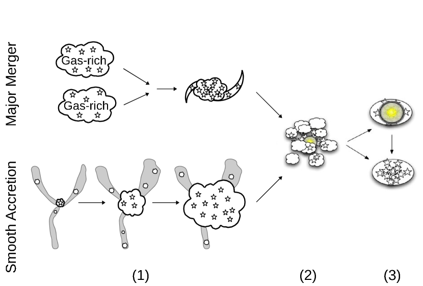
Figure 1.— Cartoon picture illustrating two possible evolutionary paths for massive galaxies at $z\sim 2$ (adapted from Dey & The NDWFS/MIPS Collaboration 2009). Top: (1) A gas rich major merger leads to an intense, dust-enshrouded phase of star-formation. (2) Energetic feedback, possibly from the growth of a central super-massive black hole, heats the dust and gas, cutting off star-formation. (3) Depending on the relative timescales of AGN fuelling, dust dissipation, and star formation, the system may be briefly visible as a quasar before settling on the red sequence. Bottom: An alternative scenario in which massive galaxies are assembled via smooth accretion of gas and small satellites along filamentary structures (some mechanism is still needed to quench star-formation; in this cartoon picture, steps (2) and (3) are assumed to be the same as in the major merger driven scenario). One goal of this paper is to test the two different possibilities illustrated in step (1) of this diagram using the stellar masses and star-formation rates of high redshift ULIRGs.

Studies attempting to connect the mid-IR and far-IR selected ULIRG population at high redshift have so far focused on their basic properties such as bolometric luminosities (Sajina et al. 2008; Coppin et al. 2008; Lonsdale et al. 2009; Bussmann et al. 2009b; Fiolet et al. 2009), clustering strengths (Blain et al. 2004; Brodwin et al. 2008), and morphologies. In particular, high-spatial resolution imaging (Dasyra et al. 2008; Melbourne et al. 2008, 2009; Bussmann et al. 2009a; Swinbank et al. 2010) and dynamics (Tacconi et al. 2006, 2008; Melbourne et al. 2011) have shown no distinction in axial ratio that might be suggestive of orientation effects; instead, these studies have identified morphological trends which are consistent with an evolutionary scenario driven by major mergers in which sources that show a bump in their mid-IR SED (i.e., bump DOGs and most SMGs) evolve into those with a power-law dominated mid-IR SED (i.e., power-law DOGs Bussmann et al. 2011). To test the origins of these sources further, it is imperative to use alternative, complementary methods of constraining the SFHs of DOGs and SMGs at $z\sim 2$.

This paper is focused on one such technique: stellar population synthesis (SPS) modeling of broad band photometry of DOGs and SMGs with known spectroscopic redshifts. The primary goal of this study is to place the tightest constraints possible given the existing data on the stellar masses ($M_{*}$) and SFHs of bump DOGs, power-law DOGs, and SMGs using a uniform SPS modeling analysis with common model assumptions and fitting techniques for each ULIRG population. There are several reasons to pursue this goal.

First, constraints on the $M_{*}$ values and SFHs of Spitzer-selected ULIRGs are limited to a few studies that have focused on bump sources (Berta et al. 2007; Lonsdale et al. 2009). In contrast, the constraints on $M_{*}$ and SFHs presented here for power-law DOGs are the first such results for this potentially very important population of galaxies. If power-law DOGs do not have significantly different masses than SMGs or bump DOGs, this might imply that the power-law phase occurs during the same time that most of the mass in stars is being built up. If the power-law is a signature of black hole growth, then this would mean that the stellar mass and black hole mass are likely being assembled during the same period of dust-obscured, intense star-formation. A uniform analysis of all three populations is necessary to test this hypothesis.

Second, while SPS modeling methods have become more sophisticated, stellar mass results for a given population have not necessarily converged. For example, Borys et al. (2005) use Spitzer/Infrared Array Camera (IRAC; Fazio et al. 2004) data to infer average SMG stellar masses of $M_{*}\approx 2.5\times 10^{11}~{}M_{\sun}$. More recently, Dye et al. (2008) and Michałowski et al. (2010) have found median stellar masses for SMGs of $M_{*}=6.3\times 10^{11}~{}M_{\sun}$ and $3.5\times 10^{11}~{}M_{\sun}$, respectively. A new study by Hainline et al. (2011) using essentially the same data set as Michałowski et al. (2010) finds significantly lower median SMG stellar masses of $M_{*}=(7\pm 3)\times 10^{10}~{}M_{\sun}$. Finally, measurements of the width of CO emission lines in 12 ULIRGs at $z\sim 2$ have provided a median dynamical mass estimate of $M_{\rm dyn}\sim 2\times 10^{11}\>M_{\sun}$ (Engel et al. 2010). These sources typically have high gas fractions of $\approx 0.5$, implying that the stellar masses should be $M_{*}\leq 10^{11}\>M_{\sun}$. This emphasizes the significant systematics that affect stellar mass estimates based on SPS modeling and underscores the need for a uniform analysis when comparing different ULIRG populations.

Third, the disagreement in observed stellar masses has significant bearing on theoretical models for the formation of high redshift ULIRGs. As outlined earlier, the cosmological hydrodynamical simulations of Davé et al. (2010) predict that SMGs have large stellar masses that are roughly consistent with the estimates of Borys et al. (2005) and Michałowski et al. (2010), but a factor of $\approx 4$ larger than the estimates of Hainline et al. (2011). The Hainline et al. (2011) mass estimates are also somewhat lower than what is expectated from merger simulations (Narayanan et al. 2010), with the caveat that such expectations are highly dependent on the stage of the merger, viewing angle, etc. A systematic, uniform comparison of the relative stellar mass distributions of DOGs and SMGs with simulated SFHs from theoretical models for the evolution of massive galaxies represents a significant component of this paper.

In section 2, we present the data used in this analysis, including DOG SEDs from rest-frame ultra-violet (UV) to near-IR. Section 3 outlines the general methodology and describes the SPS libraries, initial mass functions (IMFs), and SFHs that are used in the analysis. We present our results in section 4, including constraints on stellar masses, visual extinctions, and stellar population ages. In section 5, we compare our results with similar studies of SMGs and other Spitzer-selected ULIRGs and explain the implications of the results for models of galaxy evolution. Conclusions are presented in section 6.

Throughout this paper we assume a cosmology in which $H_{0}=$70 km s^-1 Mpc^-1, $\Omega_{\rm m}=0.3$, and $\Omega_{\Lambda}=0.7$. All magnitudes are in the AB system.

2. Data

The goal of this paper is to study the relative mass distributions of samples of high-$z$ ULIRGs, specifically DOGs and SMGs, via population synthesis modeling of their rest-frame UV through near-IR SEDs. To minimize degeneracies in the models, it is important to limit the analysis to sources with spectroscopic redshifts. Thus, the present sample consists of ULIRGs with spectroscopic redshifts at $z>1.4$ and broad-band photometry from the rest-frame UV through near-IR. The sample comprises three main sub-groups: two selected with Spitzer at 24$\mu$m (DOGs), and one selected with the Sub-mm Common User Bolometer Array (SCUBA) at 850$\mu$m (SMGs).

2.1. DOGs

2.1.1 Sample Selection

For the Spitzer-selected ULIRGs, a total of 2603 DOGs satisfying $R-[24]>14$ (Vega mag) and $F_{\rm 24\mu m}>0.3\>$mJy were identified in the 8.6 deg² NDWFS Boötes field with deep Spitzer/MIPS 24$\mu$m coverage (Dey et al. 2008). This paper focuses on the subset of 90 of these objects that have known spectroscopic redshifts at $z>1.4$ either from observations with the Keck telescope ($\approx 60\%$, Soifer et al., in prep., 2011) or with the InfraRed Spectrometer (IRS Houck et al. 2004) onboard Spitzer (Houck et al. 2005; Weedman et al. 2006b). Spectroscopic redshifts for our sample of DOGs are given in Table 1.

Figure 2 shows the $R-[24]$ color as a function of 24$\mu$m magnitude for the subsample studied here (the “spectroscopic sample”) in comparison to the overall sample of DOGs in Boötes. To optimize the spectroscopic detection rate, the spectroscopic sample is biased towards bright 24$\mu$m sources, although the full range of $R-[24]$ colors is sampled. The spectroscopic sample consists of 39 star-formation dominated “bump” sources (those that show a peak at rest-frame 1.6$\mu$m) and 51 active galactic nucleus (AGN) dominated “power-law” sources. Bump and power-law DOGs are separated according to the statistical criteria given in section 3.1.2 of Dey et al. (2008). Also shown in this diagram are 53 sub-millimeter galaxies (SMGs) with spectroscopic redshifts from Chapman et al. (2005) (see section 2.2). The redshift distributions of these groups of galaxies are shown in Figure 3. The positions, $R-[24]$ colors, and nature of mid-IR SED for each DOG in the sample are given in Table 1.

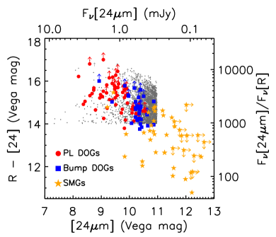
Figure 2.— $R-[24]$ color vs. 24$\mu$m magnitude distribution for DOGs in the NDWFS Boötes field. Gray dots and upward arrows show the full sample of DOGs, with and without an $R$-band detection (2$\sigma$ limits), respectively. Highlighted are the subsamples with spectroscopic redshifts and either a mid-IR power-law SED (PL DOGs, red circles) or a mid-IR bump SED (Bump DOGs, blue squares). Also shown are SMGs (orange stars) with spectroscopic redshifts from Chapman et al. (2005) and 24$\mu$m photometry from Hainline et al. (2009).

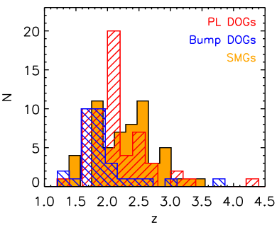
Figure 3.— Redshift distribution of DOGs in the Boötes Field with spectroscopic redshifts. The redshift distribution of bump DOGs (blue hatched) is relatively narrow due to selection effects (for details see Desai et al. 2009), while power-law DOGs (red hatched) are weighted towards slightly larger redshifts. Also shown is the redshift distribution of SMGs (orange filled region) from Chapman et al. (2005).

2.1.2 Optical Photometry

The NOAO Deep Wide Field Survey (NDWFS; Jannuzi & Dey 1999) is a ground-based optical and near-IR imaging survey of two 9.3 deg² fields, one in Boötes and one in Cetus. In this paper, we utilize the optical imaging of the Boötes field, conducted using the NOAO 4m telescope on Kitt Peak. The survey reaches 5$\sigma$ point-source depths in $B_{W}$, $R$, and $I$ of 27.1, 26.1, and 25.4 (Vega mag), respectively. The NDWFS astrometry is tied to the reference frame defined by stars from the United States Naval Observatory A-2 catalog. NDWFS data products are publicly available via the NOAO science archive .

Photometry for each DOG was measured in 4$\arcsec$ diameter apertures, centered on the 3.6$\mu$m centroid position measured from the Spitzer Deep Wide-field Survey (SDWFS; Ashby et al. 2009) imaging data (Ashby et al. 2009). Foreground and background objects were removed using SExtractor segmentation maps, and the sky level was determined using an annulus with an inner diameter of 6$\arcsec$ and a width of 5$\arcsec$. The background level and photometric uncertainty were computed by measuring the sigma-clipped mean and RMS of fluxes measured in roughly fifty 4$\arcsec$ diameter apertures within 1$\arcmin$ of the target. Aperture corrections were derived using bright, non-saturated stars for each of the 27 sub-fields that comprise the NDWFS.

2.1.3 Near-Infrared Photometry

The NOAO Extremely Wide Field InfraRed iMager (NEWFIRM) has conducted a survey at near-IR wavelengths of the full 9.3 deg² Boötes field using the NOAO 4m telescope on Kitt Peak during the spring semesters of 2008 and 2009. The nominal 5$\sigma$ limits of the survey within a 3$\arcsec$ diameter aperture in $J$, $H$, and $Ks$ are 22.05, 21.3, and 19.8 (Vega mag), respectively. All of the survey data are publicly available (Gonzalez et al., in prep.).

Photometry was computed in the same manner as with the NDWFS images (see section 2.1.2). Aperture corrections were computed using bright, non-saturated stars for each of the 52 sub-fields that comprise the NEWFIRM survey of Boötes. Photometry in the optical and near-IR is presented in Table 2.

2.1.4 Mid-Infrared Photometry

The SDWFS is a four-epoch survey of roughly 8.5 deg² of the Boötes field of the NDWFS. The first epoch of the survey took place in 2004 January as part of the IRAC Shallow Survey (Eisenhardt et al. 2004). Subsequent visits to the field as part of the SDWFS program reimaged the same area three times to the same depth each time. The final co-added images have 5$\sigma$ depths (aperture-corrected from a 4$\arcsec$ diameter aperture) of 19.77, 18.83, 16.50, and 15.85 (Vega mag) at 3.6$\mu$m, 4.5$\mu$m, 5.8$\mu$m, and 8.0$\mu$m, respectively. All SDWFS data are publicly available.

Part of the SDWFS Data Release 1.1 includes band-matched catalogs created with Source Extractor (SExtractor, Bertin & Arnouts 1996). Astrometry in these catalogs is tied to 2MASS positions within 0$\farcs$2. We identify DOGs in these catalogs using a 3$\arcsec$ search radius, and use the values in these catalogs for our flux density measurements of DOGs. SExtractor underestimates the true magnitude uncertainties because it assumes a Gaussian noise distribution where noise is uncorrelated. In place of the SExtractor-derived values, we determine our own estimates of the uncertainty on each flux density measurement using 4$\arcsec$ diameter apertures randomly placed within 1$\arcmin$ of each object of interest. Photometry in the mid-IR is presented in Table 2.

2.2. SMGs

2.2.1 Sample Selection

For the SCUBA-selected SMGs, we use the sample of 53 objects with spectroscopic redshifts at $z>1.4$ (we have removed from the sample three sources with extremely blue rest-frame ultra-violet colors as well as two sources which were subsequently shown to be spurious detections by Hainline et al. (2011)) from Chapman et al. (2005). These are sources with precise positional information derived from Very Large Array 1.4 GHz imaging and redshifts obtained with optical ground-based spectroscopy with the Keck I telescope. Their clustering properties indicate they inhabit very massive dark matter haloes ($M_{\rm DM}\approx 10^{12}\>M_{\sun}$; Blain et al. 2004), comparable to the dark matter halo masses of DOGs (Brodwin et al. 2008).

2.2.2 SMG Photometry

The broad-band photometry of SMGs used in this paper has been collected from a variety of sources. $B$- and $R$-band photometry were obtained with several telescopes and were presented in Chapman et al. (2005). $I$-, $J$-, and $K$-band photometry also were obtained with several telescopes and were presented in Smail et al. (2004). These photometry values were derived with 4$\arcsec$ diameter apertures and have been aperture-corrected. Mid-IR photometry of SMGs was obtained from Hainline et al. (2009), who compute aperture-corrected 4$\arcsec$ diameter aperture photometry using SExtractor.

3. Stellar Population Synthesis Models

Stellar population synthesis (SPS) modeling offers a means of constraining the mass and star-formation history of a galaxy’s stellar population. This section contains a description of the technique adopted here to apply the SPS models to the high-$z$ ULIRG photometry outlined in section 2. Additionally, details are provided regarding three SFHs and three initial mass functions (IMFs) that are used in this paper for testing theories for the formation of massive galaxies at high redshift. Results from this analysis are presented in section 4. A detailed analysis of the differences in $M_{*}$ measurements obtained with four SPS libraries may be found in Appendix A.

3.1. General Methodology

SPS models are parameterized at minimum by their luminosity-weighted age and their stellar mass, $M_{*}$. The attenuation of stellar light by dust adds a third parameter, $A_{V}$. In all models used here, the simplifying assumption of a uniform dust screen ($A_{V}$ ranging from 0 to 3) is adopted which obscures the intrinsic stellar light according to the reddening law for starbursts from Calzetti et al. (2000) for wavelengths between $0.12-2.2\>\mu$m and that of Draine (2003) for longer wavelengths. The available data do not allow constraints to be placed on more complex models in which younger stars have different dust obscuration prescriptions than older stars (e.g., Charlot & Fall 2000).

The broad band photometry used here is not sufficient to break the degeneracy between age and $A_{V}$ (except under special assumptions). For this reason, the main goal here is to measure the relative $M_{*}$ values of three distinct populations of high redshift ULIRGs (power-law DOGs, bump DOGs, and SMGs) using a uniform, self-consistent analysis. This will allow the stellar masses of these objects to be measured in a relative sense and therefore minimize many of the uncertainties discussed above (however, note that the masses of the power-law DOGs in general are upper limits since the AGN contribution to the 3.6$\mu$m and 4.5$\mu$m IRAC channels is unknown). Furthermore, competing models of galaxy formation and evolution make different predictions about the stellar mass properties of the most luminous galaxies at $z\sim 2$. The distribution of stellar masses of populations of power-law DOGs, bump DOGs, and SMGs is therefore (in principle) a viable tool with which to test these competing models.

The approach used here is to apply SPS models of varying $A_{V}$ and age values to generate a probility density function for the stellar mass of each galaxy, $\phi(M_{*},{\rm age},A_{V})$. $\phi(M_{*},{\rm age},A_{V})$ is computed directly from the best-fit $\chi^{2}$ value for the given number of degrees of freedom, $N_{\rm DOF}$. Since we have 7 data points and 3 model parameters, $N_{\rm DOF}=4$. For a few sources (SST24J 142648.9+332927, SMMJ030227.73+000653.5, SMMJ123600.15+621047.2, SMMJ123606.85+621021.4, SMMJ131239.14+424155.7, SMMJ163631.47+405546.9, SMMJ221735.15+001537.2, SMMJ221804.42+002154.4), no models achieved statistically acceptable fits. These systems are assumed to have a uniform stellar mass probability density function between $10^{10}-10^{12}~{}M_{\sun}$. This has the effect of broadening the resulting stellar mass constraints for a given galaxy population. Each individual galaxy’s $\phi(M_{*},{\rm age},A_{V})$ is normalized such that it contributes equally to the final stellar mass probability density function for that population of galaxies ($\phi_{\rm PLDOG}$, $\phi_{\rm BumpDOG}$, and $\phi_{\rm SMG}$).

The use of SPS models to determine intrinsic properties of galaxies assumes that all of the observed flux is emitted by stars. In fact, many of the sources in this study have a significant contribution in the rest-frame near-IR from obscured AGN (this is especially true for the power-law DOGs). Some authors add this component (in the form of a variable slope power-law) to their SPS modelling efforts (e.g., Hainline et al. 2011). Alternatively, it is possible to minimize the AGN contribution by considering only the first two IRAC channels (i.e., up to observed-frame 4.5$\mu$m). We adopt the latter approach in this study. For bump DOGs and most SMGs, this should provide a reasonably reliable measurement of the stellar light from these objects. For power-law DOGs and those SMGs with power-law tails in the near-IR, there still exists a significant possibility that the observed-frame 4.5$\mu$m light is contaminated by AGN, though it should be noted that high-spatial resolution imaging with HST/NICMOS indicates that only 10-20% of the rest-frame optical light is emitted by a point source in power-law DOGs (Bussmann et al. 2009a). For this reason, the stellar mass estimates of power-law DOGs should be regarded as upper limits on the true stellar mass.

The observed-frame $B_{W}$ photometry have been excluded from the fitting process. These data typically probe rest-frame 1500 Å and as such are highly sensitive to the youngest stellar populations and the detailed geometry of the dust distribution surrounding them. The most robust model fits were obtained when the $B_{W}$ photometry were not used.

Only solar metallicity models are tested in this study. This is a reasonable assumption, since high-redshift (median redshift of 2.4) dusty galaxies have been found to have near-solar metallicities (Swinbank et al. 2004). Moreover, our broad-band SED data do not provide the ability to constrain metallicity. The adoption of a single metallicity in SPS modeling typically introduces uncertainties at the level of 10-20% (Conroy et al. 2009; Muzzin et al. 2009), which are insignificant compared to systematic uncertainties related to the IMF, SFH, and age of the stellar population.

3.2. SPS Star-formation Histories

One of the most critical adjustable parameters in SPS modeling is the star-formation history (SFH). Michałowski et al. (2011) suggest that the use of multiple component SFHs, in which different stellar populations are allowed to have distinct ages and obscuration, can lead to factors of 2-4 difference in best-fit stellar mass. The focus in this paper is placed on three distinct SFHs that broadly encompass a reasonable range of parameter space while maintaining a level of simplicity in accordance with the quality of the available data.

The first SFH adopted here is the simplest one possible: an infinitely short burst of star-formation at time $t=0$ during which all the stars of the galaxy are formed, followed thereafter by passive evolution. This is called a simple stellar population (SSP), and is used commonly in SPS modeling in the literature. If the objects under study here have recently had star-formation shut off by some process (e.g., AGN feedback), then the SSP model provides constraints on how long ago such an event ocurred. Models used here have ages spaced logarithmically from 10 Myr up to 1 Gyr.

The second SFH used in this paper is borrowed from a representative simulation of a major merger which undergoes a very luminous sub-mm phase (SMG) as well as a highly dust-obscured phase (DOG) before star-formation is shut off by AGN feedback effects (Narayanan et al. 2010). This SFH traces the star-formation rate from the beginning of the simulation — before the two gas-rich ($f_{g}\sim 0.8$) disks begin to interact — through the period of final coalescence when the SFR peaks near 1000 $M_{\sun}\>$yr^-1, to the end of the simulation and a red, dead, elliptical galaxy. Models used here have ages spaced roughly linearly from 10 Myr to 0.8 Gyr.

The third SFH adopted in this study comes from cosmological hydrodynamical simulations in which SMGs are posited to correspond to the most rapidly star-forming systems that match the observed number density of SMGs (Davé et al. 2010). In particular, the SFH and metallicity history of the highest SFR simulated SMG are used. This object has a SFR of $\approx 150~{}M_{\sun}\>$yr^-1 for most of the simulation but is boosted to $\approx 500~{}M_{\sun}\>$yr^-1 at $z=2$ and reaches a mass of $M_{*}=2.8\times 10^{11}~{}M_{\sun}$ by the same redshift. As nearly all of the mass is assembled in a quiescent mode, this SFH is nearly opposite to a SSP, in which all stars are formed in a single infinitely short burst. Models used here have ages spaced roughly linearly over the full range of the SFH, from 10 Myr to 3 Gyr. Figure 4 shows the SFHs from Narayanan et al. (2010) and Davé et al. (2010) that are used in this analysis.

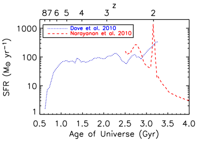
Figure 4.— Star-formation histories used in stellar population synthesis models. Dotted line represents high-$z$ ULIRGs identified in cosmological hydrodynamical simulations formed via smooth gas inflow and accretion of small satellites (Galaxy A from Figure 4 of Davé et al. 2010). Dashed line represents high-$z$ ULIRGs formed via major mergers of two gas-rich disks (Narayanan et al. 2010) and has been shifted in time so that the peak star-formation rate occurs at $z\approx 2$.

3.3. Initial Mass Functions

Another critical adjustable parameter involved in SPS modeling is the IMF. Despite its importance, the detailed nature of the IMF in galaxies at high redshift is poorly constrained. The relevant parameter space is characterized here by three different forms: a Salpeter IMF (Salpeter 1955), a Chabrier IMF (Chabrier 2003), and a bottom-light IMF (e.g., van Dokkum 2008; Davé 2008). All of these have a lower mass cutoff of 0.1 $M_{\sun}$ and an upper mass cutoff of 100 $M_{\sun}$. The Chabrier IMF has fewer low mass stars compared to a Salpeter IMF (and hence a lower mass-to-light ratio), while a bottom-light IMF has even fewer low-mass stars (and a correspondingly lower mass-to-light ratio).

The contribution of low mass stars to the bottom-light IMF is governed by the characteristic mass, $m_{c}$, which controls both the cutoff mass at which the lognormal form dominates as well as the shape of the lognormal part of the IMF itself. In particular, van Dokkum (2008) use the color and luminosity evolution of cluster ellipticals to infer $m_{c}\sim 2~{}M_{\sun}$ at $z>4$ (however, see van Dokkum & Conroy 2010, which argues instead for a steeper-than-Salpeter IMF slope based upon spectral features that are strong in stars with $M_{*}<0.3\>M_{\sun}$ found in elliptical galaxies in the local Universe). In this study, a characteristic mass of $m_{c}=0.4~{}M_{\sun}$ has been adopted, as this value matches both the (very rough) estimates for SMGs at $z\sim 2$ as well as theoretical expectations based on a model in which the characteristic mass is a function of the CMB temperature: $m_{c}\propto T_{\rm CMB}^{3.35}$. The effect of such a change in the characteristic mass is to produce a Salpeter-like slope at $M>1~{}M_{\sun}$ and a turnover at $M\approx 1~{}M_{\sun}$. This reduces the number of low-mass stars relative to the high-mass ones, thereby lowering the mass-to-light ratio relative to the Chabrier IMF (for intermediate age stars or younger).

Since observational constraints on the IMF are not readily available, each IMF has been tested with each SFH (see section 3.2). In the case of the simple stellar population (SSP), this provides a measure of the uncertainty resulting from the unknown IMF. However, for the purposes of testing the self-consistency of more complicated SFHs of ULIRGs at high redshift, it is necessary to select certain IMFs for each model. The simulations of major mergers tested here (Narayanan et al. 2010) adopt a Kroupa IMF for their radiative transfer, so a Chabrier IMF (which is very similar to a Kroupa IMF) is what is focused on here. Meanwhile, the IMF is a free parameter in the smooth accretion SFH (Davé et al. 2010). A Chabrier IMF is adopted in this paper for this SFH (with an accompanying thorough discussion of the implications of a more “bottom-light” IMF), since a Salpeter IMF overpredicts the sub-mm fluxes of SMGs.

4. Results

This section presents measurements of the stellar masses ($M_{*}$) of bump DOGs, power-law DOGs, and SMGs. SEDs for each source may be found in Appendix B. The nominal fiducial model chosen in this paper is the CB07 SPS library with a SSP SFH and Chabrier IMF (meaning that we have chosen this as the standard by which the other models will be compared), and is presented in section 4.1. In later sections, alternative SFHs and IMFs are explored. Although differences exist between various SPS libraries in the treatment of aspects of stellar atmospheres and evolution, these details are sub-dominant to the choice of SFH and IMF (for an explanation of this, see Appendix A). For this reason, our modeling process does not include marginalization over SPS library.

4.1. Simple Stellar Population

The SSP represents a SFH in which all stars form in an infinitely short burst of star-formation and evolve passively thereafter. While this is an idealized scenario for the formation of massive galaxies, it is worth studying since SSPs form the building blocks of more complex SFHs and can be used more directly to compare the effect of different SPS libraries and IMFs (see section 4.4 for more details on this last point).

Figure 5 shows the stellar mass probability density function resulting from fitting a SSP (computed with the CB07 SPS library and a Chabrier IMF) to each power-law DOG, bump DOG, and SMG. All three populations have a similar range of acceptable $M_{*}$ values. Power-law DOGs tend to be the most massive systems, followed by bump DOGs and then SMGs. However, their median stellar masses are separated by $\approx 0.1$ to 0.2 dex, while the spread in their distributions are $\approx 0.3$ dex. This implies that the differences in stellar mass between the populations are suggestive rather than conclusive. Perhaps the most interesting feature of this result is that the masses of all three populations are not significantly different. This may imply that that the power-law phase occurs during the same time that most of the mass in stars is being built up. If the mid-IR power-law is a signature of black hole growth, then this implies that the stellar mass and black hole mass are being assembled during the same period of dust-obscured, intense star-formation. A low mass tail is present in each population which is in fact a reflection of the fact that the constraints on the stellar mass of a small percentage of each group are weak. The median and inter-quartile range of stellar masses for this SPS model are given in Table 3.

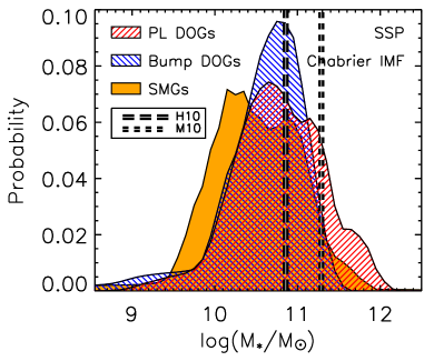
Figure 5.— Stellar mass probability density function of power-law DOGs (red), bump DOGs (blue), and SMGs (orange) derived using using the CB07 library, a Chabrier IMF, and a simple stellar population SFH. The median $M_{*}$ value (corrected to a Chabrier IMF) from studies by Hainline et al. (2011) and Michałowski et al. (2010) are given by the long and short dashed lines, respectively. The mass estimates presented here indicate both types of DOGs have masses similar to SMGs and are closer to the Hainline et al. (2011) values than those of Michałowski et al. (2010).

One feature of the fitting process that is not shown in Figure 5 is the well-known significant degeneracy between $A_{V}$ and stellar age – the broad-band photometry of these high-$z$ ULIRGs can be fit either by young (10 Myr) and dusty ($A_{V}\sim 1.5-2$) stellar populations or intermediate age (500 Myr) and less dusty ($A_{V}\sim 0.0-0.5$) stellar populations. Given the large quantities of dust that are known to exist in these systems based on observations at longer wavelengths (e.g., Kovács et al. 2006; Coppin et al. 2008; Bussmann et al. 2009a; Lonsdale et al. 2009; Kovács et al. 2010), it is unlikely that $A_{V}<1$ solutions are acceptable. Indeed, mid-IR spectra of Spitzer-selected ULIRGs generally show strong silicate absorption features indicative of highly obscured sources (Sajina et al. 2007). Furthermore, measurements of H$\alpha$ and H$\beta$ in a handful of sources find strong Balmer decrements implying $A_{V}>1$ (Brand et al. 2007).

Assuming $A_{V}=E(B-V)/R_{V}$ (where $R_{V}=3.1$) and the relation between $E(B-V)$ and the hydrogen column density ($N_{\rm H}$) from Bohlin et al. (1978), $A_{V}\sim 1$ implies $N_{\rm H}\sim 2\times 10^{21}~{}$cm^-2. Under the assumption of a spherical shell around the source with radius equal to the effective radius ($R_{\rm eff}$), the dust mass can be estimated from $N_{\rm H}$ using:

$$M_{\rm d}=\frac{1}{f_{\rm gd}}\mu_{\rm p}N_{\rm H}4\pi R_{\rm eff}^{2},$$ (1)

where $f_{\rm gd}$ is the gas-to-dust mass ratio (assumed to be 60, the value found appropriate for SMGs; Kovács et al. 2006) and $\mu_{\rm p}$ is the mean molecular weight of the gas (assumed to be 1.6 times the mass of a proton). Morphological measurements indicate these objects have typical effective radii of 3-8 kpc (Dasyra et al. 2008; Bussmann et al. 2009a; Donley et al. 2010). All together this implies $M_{\rm d}\sim(0.5-3)\times 10^{8}~{}M_{\sun}$, depending on the size of $R_{\rm eff}$. In fact, based on 350$\mu$m observations, Kovács et al. (2010) find dust masses of $M_{\rm d}\approx(5-10)\times 10^{8}~{}M_{\sun}$ for Spitzer-selected ULIRGs with a mid-IR bump feature. This suggests that $A_{V}>1$ and hence age $<200$ Myr models should be preferred. Note however that for any given galaxy, we do not have independent constraints on $A_{V}$ and hence have applied no priors on this quantity in the fitting process.

4.2. Merger-Driven Star-Formation History

One of the major goals of this paper is to go beyond instantaneous burst SFHs (SSPs) and test the self-consistency of more complicated SFHs. Two in particular that are tested here are a SFH driven by a major merger (Narayanan et al. 2010) and a SFH driven mainly by smooth accretion of gas and nearby small satellites (Davé et al. 2010). The merger-driven SFH is described here, while the smooth accretion SFH is described in section 4.3.

Figure 6 (left panel) shows the stellar mass probability density function for power-law DOGs, bump DOGs, and SMGs derived using a merger-driven SFH (from Narayanan et al. 2010) with the CB07 SPS library and a Chabrier IMF. The median and inter-quartile range of $M_{*}$ values are given for this SFH in Table 3 and are about 0.1-0.2 dex larger than the same values derived using a SSP and a Chabrier IMF (again the trend in masses is that power-law DOGs are the most massive and SMGs the least massive, with bump DOGs falling in between). Multi-component SFHs in general produce higher mass-to-light ratios than SSPs because even a modest amount of rest-frame UV emission will strongly constrain the age of the SSP to be less than a few hundred million years. Such a young stellar population will have a low mass-to-light ratio. In contrast, a multi-component SFH can have a low mass young stellar component (which reproduces the rest-frame UV emission) as well as an old stellar component which boosts the mass-to-light ratio.

This point is made more clearly in the right panel of Figure 6, which shows the stellar mass probability density function for power-law DOGs, bump DOGs, and SMGs derived from the merger-driven SFH but focusing on the portion of the SFH when the system is expected to be in its ULIRG phase (i.e., maximum SFR). By this stage (about 0.7 Gyr into the SFH), the presence of a significant amount of low mass stars increases the inferred stellar masses by 0.1-0.3 dex (relative to the masses derived from the SSP SFH). These mass estimates are also reported in Table 3. The increase in our estimates of $M_{*}$ is actually mitigated somewhat because the SFR is so high that the fraction of very massive stars relative to all other stars is higher than at other times in the SFH and because we have made the simplest possible assumption for the dust geometry of a uniform dust screen. In reality, the youngest stars should experience greater extinction than the older stars. This effect is likely to be amplified by the merger, in which the peak SFR occurs when all the gas and dust have been dumped into the central, most obscured regions. For this reason, we expect that our measurements of $M_{*}$ for the merger SFH during this period are likely to underestimate the true stellar masses.

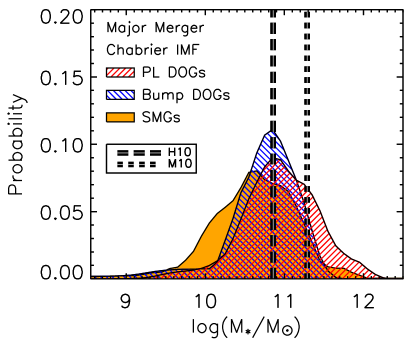
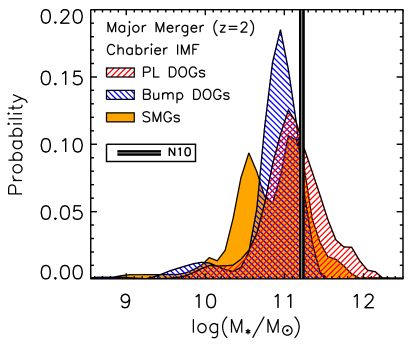
Figure 6.— Similar to Figure 5, but assuming a major merger SFH (see Figure 4 of this paper and Narayanan et al. 2010). Left: Stellar masses obtained when marginalizing over the full age range of the model. Mass estimates from Hainline et al. (2011) and Michałowski et al. (2010) (dashed and dotted lines, respectively) have been corrected to a Chabrier IMF. Right: Stellar masses obtained when marginalizing over only the $z=2$ period of the model (i.e., the timestep during which the SFR peaks). When only the $z=2$ period is considered, the inferred stellar masses increase by 0.1-0.3 dex (see Table 3) thanks to the increased contribution from old stars with high mass-to-light ratios. The median stellar masses of these $z\sim 2$ ULIRGs are still about 0.2-0.3 dex lower than expected from the Narayanan et al. (2010) models (solid line).

It is somewhat interesting that a bimodal distribution in SMG stellar masses appears when one focuses on the period of peak SFR in the merger simulation. This bimodality is smoothed out in the left panel of Figure 6, which shows the superposition of all ages during the SFH. The origin of the bimodality is not entirely clear, but is likely due to the presence of a significant number of SMGs that are rest-frame UV-bright and therefore are found to have relatively low stellar masses. In contrast, DOGs are selected to be rest-frame UV-faint and do not show this bimodality in stellar masses.

4.3. Smooth Accretion Star-Formation History

In the cosmological hydrodynamical simulations of Davé et al. (2010), SMGs are posited to be the maximally star-forming galaxies whose number densities match the observed number density of SMGs. This results in the typical simulated SMG having a SFH described by a relatively constant SFR of 100-200 $M_{\sun}~{}$yr^-1 over a period of 3 Gyr and leads to a stellar mass in these systems in the range $M_{\sun}\approx(1-5)\times 10^{11}~{}M_{\sun}$. Davé et al. (2010) note that their simulated SFRs are a factor of $\sim 3$ lower than the typical values observationally inferred for SMGs, and hypothesize that a “bottom-light” IMF such as that proposed by van Dokkum (2008) and Davé (2008) could explain this discrepancy. This type of IMF would also have the consequence of modifying the $M_{*}/L_{V}$ of the galaxy, meaning that at a given $L_{V}$, the inferred stellar mass will be lower than for other IMFs such as Chabrier or Salpeter. It is for this reason that the constraints on the stellar masses of the high-$z$ ULIRGs with this SFH are of particular interest.

Figure 7 (left panel) shows the stellar mass probability density function for power-law DOGs, bump DOGs, and SMGs derived using a SFH driven mainly by smooth accretion of gas and nearby satellites (with the CB07 SPS library and a Chabrier IMF). The median and inter-quartile range of $M_{*}$ estimates are provided in Table 3. In this case, the median stellar masses of the three populations are separated by $\approx 0.15$ dex, with power-law DOGs being the most massive and SMGs being the least massive (note that this is still well below the typical inter-quartile range in the stellar mass estimates of $\approx 0.3$ dex). In comparison to the SSP SFH, the smooth accretion mass estimates are $\approx 0.2$ dex larger, for similar reasons as those outlined at the end of section 4.2.

Restricting the age range of the SFH for the smooth accretion model to coincide with the period during which the simulated systems are expected to be ULIRGs (i.e., at $z\sim 2-3$) leads to inferred stellar masses that are larger by 0.3-0.4 dex compared to the SSP SFH (Table 3 and Figure 7, right panel). As described in section 4.2, this is a result of a greater contribution from older stars that have higher mass-to-light ratios than younger stars.

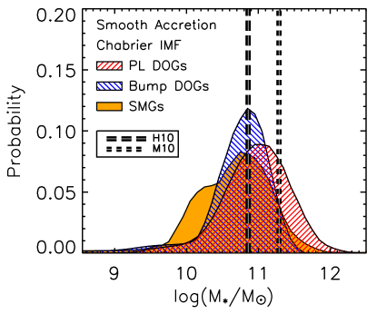
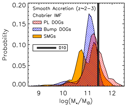
Figure 7.— Similar to Figure 5, but assuming a smooth accretion SFH (see Figure 4 of this paper and Davé et al. 2010). Left: Stellar masses obtained when marginalizing over the full age range of the model. Right: Stellar masses obtained when marginalizing over only the $z\sim 2-3$ period of the model. Here, the stellar mass values increase by 0.3-0.4 dex when only the $z\sim 2$ epoch of the SFH is considered due to the increased contribution of low-mass stars which have high mass-to-light ratios. The median stellar masses of these $z\sim 2$ ULIRGs are still about 0.3-0.4 dex lower than expected from the Davé et al. (2010) models (solid line).

4.4. Variation with IMF

In SPS modeling, the IMF affects primarily the mass-to-light ratio of the synthesized stellar population. Bruzual & Charlot (2003) showed that the $B-V$ and $V-K$ colors of SPS models distinguished only by their IMFs (Chabrier vs. Salpeter) are very similar. On the other hand, the Salpeter IMF gives mass-to-light ratios that are $\approx 0.2$ dex larger than the Chabrier IMF. Bottom-light IMFs (such as that advocated by van Dokkum 2008) have more complicated mass-to-light ratios that depend on both the characteristic mass ($m_{c}$) and the age of the stellar population. van Dokkum (2008) find that for $m_{c}=0.4~{}M_{\sun}$ (as adopted here) and ages $<1~{}$Gyr, the mass-to-light ratio is lower by 0.2-0.3 dex compared to a Chabrier IMF. The results of this study are consistent with this finding: assuming a SSP SFH and this bottom-light IMF, the stellar masses of bump DOGs are in the range $M_{*}=(0.1-0.6)\times 10^{11}~{}M_{\sun}$, or about 0.3-0.4 dex lower than those inferred using a Chabrier IMF. A similar reduction in $M_{*}$ occurs when using the bottom-light IMF in conjunction with more complicated SFHs such as the merger-driven SFH and the smooth accretion SFH detailed in sections 4.2 and 4.3.

5. Discussion

The focus of this section is to build upon the constraints on the stellar masses and star-formation histories of bump DOGs, power-law DOGs, and SMGs presented in section 4. Estimates of $M_{*}$ presented here are compared with estimates of other dust-obscured high-redshift ULIRGs. In addition, implications for models of galaxy evolution are presented based upon a comparison of the two theoretical SFHs considered in this study (major merger and smooth accretion).

5.1. Comparing Stellar Mass Estimates of ULIRGs at $z\sim 2$

Studies of other Spitzer-selected ULIRGs with a bump in the observed-frame mid-IR SED have found median stellar masses of $M_{*}\approx 10^{11}~{}M_{\sun}$ (for a Chabrier IMF; Berta et al. 2007; Lonsdale et al. 2009; Huang et al. 2009). This is a little more than $1\sigma$ higher than the median stellar mass found for bump DOGs here. The small difference in stellar mass estimates can be fully accounted for by the choice of star-formation history as well as the use in this study of the new CB07 SPS libraries, which have redder near-IR colors and hence tend towards lower inferred stellar masses (see section 4.4 and also Muzzin et al. 2009).

Two recent studies of SMGs using stellar population synthesis modeling have come to differing conclusions regarding their median $M_{*}$. While Michałowski et al. (2010) find a median stellar mass of $M_{*}\approx 2\times 10^{11}~{}M_{\sun}$ (using SEDs from Iglesias-Páramo et al. 2007, and after converting to a Chabrier IMF), Hainline et al. (2011) find $M_{*}=7\times 10^{10}~{}M_{\sun}$ (assuming a Chabrier IMF and models from Maraston 2005). Hainline et al. (2011) argue that models which do not consider the contribution of an obscured AGN in the mid-IR (particularly in the 5.8$\mu$m and 8.0$\mu$m channels of IRAC) can bias stellar mass estimates of SMGs upwards by a factor of $\approx 2$. Our analysis (which excludes these two IRAC channels to minimize the contribution from an obscured AGN) indicates stellar masses that are closer to those of Hainline et al. (2011), with median $M_{*}=4.4\times 10^{10}~{}M_{\sun}$ (for a smooth accretion SFH without constraints on the age of the stellar population, which most closely resembles the SSP and constant star formation histories adopted by Hainline et al. (2011)). Inclusion of the additional two IRAC channels increases our stellar mass estimates by 50% (median $M_{*}=6\times 10^{10}~{}M_{\sun}$). A similar increase is seen when including the 5.8$\mu$m and 8.0$\mu$m channels of IRAC to models which focus on the age of the smooth accretion SFH corresponding to the ULIRG phase (i.e., $z\sim 2$). This is somewhat of a smaller effect than found by Hainline et al. (2011), possibly suggesting that there may be some contamination from AGN in the 3.6$\mu$m and 4.5$\mu$m IRAC channels that we are not accounting for as well.

5.2. Implications for Galaxy Evolution at $z\sim 2$

Observational evidence indicates that ULIRGs in the local Universe are the product of major mergers (Armus et al. 1987) and that they are connected in an evolutionary sense with quasars (Sanders et al. 1988a, b). It is tempting to postulate a similar major-merger origin for high-redshift ULIRGs. However, conclusive evidence linking variously selected ULIRG populations to each other and to quasars at high redshift requires measurements that challenge current observational capabilities. Nevertheless, some tantalizing hints exist that suggest these diverse populations are indeed linked. First, the clustering strength of DOGs is comparable to that of both the SMGs and QSOs at similar redshifts (Brodwin et al. 2008). Second, the quantitative morphologies of DOGs and SMGs are consistent with an evolutionary picture in which the SMG phase precedes the bump DOG phase, which in turn precedes the PL DOG phase (Bussmann et al. 2011). However, such morphological studies are challenging because of surface brightness dimming and dust-obscuration effects, which prevent a straightforward merger identification based on imaging (Dasyra et al. 2008; Melbourne et al. 2008; Bussmann et al. 2009a; Melbourne et al. 2009; Zamojski et al. 2011; Bussmann et al. 2011).

This study offers an independent means of testing both the evolutionary hypothesis as well as the merger hypothesis via SPS modeling of broad-band imaging in the rest-frame UV through near-IR. The approach followed in this paper is to test the self-consistency of two distinct SFHs. One is characterized by a gas-rich major merger which reaches a peak SFR of $\approx 1000~{}M_{\sun}\;$yr^-1 (Narayanan et al. 2010). The other is characterized by smooth accretion of gas and small satellites that typically reaches SFRs of $\approx 200-300~{}M_{\sun}\;$yr^-1 at $z\sim 2$ (Davé et al. 2010).

First, it is worth noting that in the model of Narayanan et al. (2010), an evolutionary progression exists in which SMGs evolve into bump DOGs which evolve into power-law DOGs. This process occurs on a short time-scale ($\sim 50-100$ years), but if it is true then we should expect the SMGs to have the youngest stellar population, followed by bump DOGs and then power-law DOGs. In this case, the relative differences in the inferred stellar masses for the three populations become more significant and in the expected direction for the evolutionary scenario outlined above. In comparison, the model of Davé et al. (2010) does not yet include radiative transfer calculations and so cannot make a prediction for an evolutionary scenario between these three populations. Because of the short timescales involved in the merger simulations and the nature of our seven filter broadband photometry dataset, we do not pursue this point in a more quantitative manner, but we nevertheless believe that it deserves mentioning.

Second, the stellar masses reported here are factors of 2-2.5 lower than expected from the both the merger and smooth accretion models tested in this paper. This reflects the large uncertainties inherent in absolute measurements of stellar mass and indicates that stellar masses alone are unlikely to provide a definitive reason to favor either model over the other. Michałowski et al. (2011) show that the use of multi-component SFHs (i.e., multiple stellar populations with varying ages, extinctions, and masses) in SPS modeling can lead to higher inferred total stellar masses by virtue of using the young stellar component to match the rest-frame UV flux and the old stellar component to match the rest-frame near-IR flux. We do not believe the data we have in hand (broad-band photometry in seven filters) is sufficient to warrant such complex models, but it is nevertheless important to recognize that such models are indeed capable of implying larger stellar masses than the models we have adopted in this paper.

In addition, the unknown form of the IMF can potentially insert another factor of 2-4 uncertainty in the absolute stellar mass measurements. However, it must be emphasized that modifications in the assumed IMF will affect not only the inferred stellar masses, but also the inferred instantaneous SFRs. Thus, the effect of the IMF can be minimized by comparing the stellar masses of $z\sim 2$ ULIRGs to their star-formation rates. Although SFRs are not yet well known in Spitzer-selected ULIRGs, early evidence indicates that bump sources may have similar SFRs as SMGs ($\sim 1000~{}M_{\sun}~{}$yr^-1 Lonsdale et al. 2009; Kovács et al. 2010), whereas power-law sources may have much lower SFRs (e.g. $\sim 100~{}M_{\sun}~{}$yr^-1; Melbourne et al. 2011).

A galaxy with a mass of $M_{*}=1\times 10^{11}\>M_{\sun}$ and a SFR of $1000~{}M_{\sun}~{}$yr^-1 has a specific SFR of ${\rm sSFR}=1\times 10^{-8}~{}{\rm yr}^{-1}$. A galaxy with a SFR lower by a factor 10 will have a sSFR that is also lower by a factor of 10. Thus the range for DOGs and SMGs in sSFR is likely to be of order $1-10~{}{\rm Gyr}^{-1}$. In comparison, simulations of major mergers that produce DOG and SMG behavior tend to have ${\rm sSFR}=6~{}{\rm Gyr}^{-1}$. On the other hand, in smooth accretion driven simulations, SMGs have ${\rm sSFR}=0.7~{}{\rm Gyr}^{-1}$. Even if we adopted assumptions regarding the SFHs and dust geometry that led to stellar masses that were a factor of 2-4 larger and were thus consistent with those found by e.g. Michałowski et al. (2010), the range in sSFR values for DOGs and SMGs would still be higher than the expectation from the smooth accretion model. This is merely a consequence of the fact that mergers provide a more ready mechanism to obtain high sSFR values than smooth accretion models.

6. Conclusions

In this paper, we analyze the broad-band SEDs of a large sample of mid-IR selected (bump and power-law DOGs) and far-IR selected (SMGs) ULIRG populations with known spectroscopic redshifts and use stellar population synthesis models to estimate self-consistently the stellar masses of these three populations. We compare our mass estimates with predictions from two competing theories for the formation of these systems and examine the implications for galaxy evolution. We list our findings below.

• The median and inter-quartile range of stellar masses for SMGs, bump DOGs and power-law DOGs are log$(M_{*}/M_{\sun})=10.71^{+0.40}_{-0.34}$, $10.62^{+0.26}_{-0.32}$, and $10.42^{+0.42}_{-0.36}$, respectively, assuming a simple stellar population SFH, a Chabrier IMF, and the CB07 stellar libraries. The overlap in $M_{*}$ values between all three populations is consistent with the picture in which they represent a brief but important phase in massive galaxy evolution, with tentative evidence supporting a scenario in which SMGs evolve into bump DOGs which evolve into power-law DOGs.

• The use of more realistic SFHs in the SPS modeling in which both old and young stars contribute to the observed broad-band photometry can increase mass estimates significantly. We show that using a major merger driven SFH during its peak SFR period (when it is expected to be identified as a ULIRG at $z\sim 2$) leads to median and inter-quartile stellar mass estimates for power-law DOGs, bump DOGs, and SMGs of log$(M_{*}/M_{\sun})=11.06^{+0.24}_{-0.21}$, $10.88^{+0.14}_{-0.13}$, and $10.86^{+0.24}_{-0.37}$, respectively. Using a smooth accretion driven SFH (focusing on the predictions at $z\sim 2$) these values become log$(M_{*}/M_{\sun})=11.20^{+0.23}_{-0.20}$, $11.03^{+0.15}_{-0.14}$, and $11.02^{+0.25}_{-0.37}$, respectively.

• The stellar masses we measure are inconsistent with those predicted by both numerical simulations we have tested (being lower by a factor of 2-2.5). This indicates that either the simulations over-predict the stellar masses of high-$z$ ULIRGs, or that one (or more) of the assumptions in our SPS models is incorrect. In either case, the stellar mass data presented here are by themselves insufficient to favor one model over another. However, we note that the use of a bottom-light rather than a Chabrier IMF may be needed for the SFRs of the smooth accretion model to match those that are observed. Such a change would decrease our mass estimates by a factor of roughly 2 (depending on the exact shape of the bottom-light IMF). This line of reasoning suggests that, at least for the most luminous sources, the smooth accretion model has difficulty reproducing the observed far-IR emission (i.e., instantaneous SFR) without overestimating the observed optical and near-IR emission (i.e., stellar mass).

Estimates of the stellar masses of dust-obscured galaxies at high-redshift are highly dependent on the age of the stellar populations within those galaxies. The use of multiple component SFHs with different ages can lead to significant variations in the inferred stellar mass (e.g., Michałowski et al. 2011). We do not consider the broad-band photometry in seven filters used here to be sufficient to explore such complex SFHs. However, in the near future, wide-field medium-band photometry surveys in the near-IR (e.g., the NEWFIRM Medium-Band Survey, NMBS; van Dokkum et al. 2009) will provide a finer sampling of the rest-frame Balmer and 4000 Å break and significantly improve constraints on the stellar population age in DOGs and SMGs. Further in the future, the advent of the James Webb Space Telescope will provide high-spatial resolution imaging in the mid-IR and provide improved constraints on the amount of stellar emission vs. AGN emission in ULIRGs at high redshift. This is critical information especially for power-law DOGs, but holds significance for bump DOGs and SMGs as well.

This work is based in part on observations made with the Spitzer Space Telescope, which is operated by the Jet Propulsion Laboratory, California Institute of Technology under NASA contract 1407. Spitzer/MIPS guaranteed time observing was used to image the Boötes field at 24$\mu$m and is critical for the selection of DOGs.

We wish to acknowledge our referee, Laura Hainline, whose comments have helped greatly to improve the clarity of the paper. We thank the SDWFS team (particularly Daniel Stern and Matt Ashby) for making the IRAC Legacy data products available to us. We are grateful to the expert assistance of the staff of Kitt Peak National Observatory where the Boötes field observations of the NDWFS were obtained. The authors thank NOAO for supporting the NOAO Deep Wide-Field Survey. In particular, we thank Ed Ajhar, Jenna Claver, Alyson Ford, Tod Lauer, Lissa Miller, Glenn Tiede and Frank Valdes and the rest of the NDWFS survey team, for their assistance with the execution of the NDWFS. We also thank the staff of the W. M. Keck Observatory, where many of the galaxy redshifts were obtained.

RSB gratefully acknowledges financial assistance from HST grants GO10890 and GO11195, without which this research would not have been possible. Support for Programs HST-GO10890 and HST-GO11195 was provided by NASA through a grant from the Space Telescope Science Institute, which is operated by the Association of Universities for Research in Astronomy, Incorporated, under NASA contract NAS5-26555. The research activities of AD and BTJ are supported by NOAO, which is operated by the Association of Universities for Research in Astronomy (AURA, inc.) under a cooperative agreement with the National Science Foundation.

Facilities used: Spitzer Space Telescope; Kitt Peak National Observatory Mayall 4m telescope; W. M. Keck Observatory; Gemini-North Observatory.

Appendix A SPS Libraries

Four SPS libraries have been tested in this analysis of the SEDs of DOGs and SMGs. The first SPS library used in this paper is from the Bruzual & Charlot (2003) population synthesis library. It uses the isochrone synthesis technique (Charlot & Bruzual 1991) and the Padova 1994 evolutionary tracks (Girardi et al. 1996) to compute the spectral evolution of stellar populations at ages between 10⁵ and $2\times 10^{10}$ yr. The STEllar LIBrary (STELIB Le Borgne et al. 2003) of stellar spectra offer a median resolving power of 2000 over the wavelength range 3200 to 9500 Å. Outside this wavelength range, the BaSeL 3.1 libraries (Westera et al. 2002) are used and offer a median resolving power of 300 from 91 Å to 160$\mu$m.

The second SPS library used here is an updated version of the Bruzual & Charlot (2003) population synthesis library (Charlot & Bruzual, private communication, hereafter CB07). The primary improvement included in these models is a new prescription for the thermally pulsing asymptotic giant branch (TP-AGB) evolution of low- and intermediate-mass stars Marigo & Girardi (2007) and Marigo et al. (2008). This has the effect of producing significantly redder near-IR colors for young and intermediate-age stellar populations, which leads to younger inferred ages and lower inferred masses for a given observed near-IR color. These new models otherwise still rely on the Padova 1994 evolutionary tracks and the combination of BaSeL 3.1 and STELIB spectral libraries.

The third SPS library employed in this paper is called a Flexible Stellar Population Synthesis library (FSPS; Conroy et al. 2009, 2010; Conroy & Gunn 2010). This library uses the isochrone synthesis technique as well, but with updated evolutionary tracks (Padova 2008 Marigo & Girardi 2007; Marigo et al. 2008). FSPS adopts the BaSeL 3.1 spectral library (Westera et al. 2002) but includes TP-AGB spectra from a compilation of more than 100 optical/near-IR spectra spanning the wavelength range 0.5 – 2.5$\mu$m (Lançon & Wood 2000; Lançon & Mouhcine 2002). One feature of this library that is not available in the others is the ability to input a custom IMF (e.g., a “bottom-light” IMF).

The fourth and final SPS library used here is from Maraston (2005). This library adopts the “fuel-consumption” approach, in which the integration variable is the amount of hydrogen or helium consumed by nuclear burning during a given post-main-sequence phase (unlike the isochrone synthesis approach, in which the integration variable is the stellar mass). This library features a strong contribution from TP-AGB stars ($\approx 40\%$ of the bolometric light) for age ranges of 0.2 - 2 Gyr. A comparison between this library and that of Bruzual & Charlot (2003) found that the near-IR colors of $z\sim 2$ galaxies were better fit by the former (Maraston et al. 2006), highlighting the importance of a proper treatment of the TP-AGB phase for intermediate age stellar populations.

Appendix B SEDs

Since every source in this study has a known spectroscopic redshift, it is possible to construct SEDs for each source showing the luminosity per unit frequency ($L_{\nu}$) as a function of rest-frame wavelength ($\lambda_{\rm rest}$). Figures 8, 9, 10 show the SEDs for power-law DOGs, bump DOGs, and SMGs, respectively. Also shown in this diagram is the best-fit synthesized stellar population model (CB07, simple stellar population, Chabrier IMF). Inset in each diagram is the stellar mass probability density function. In a few cases (SST24J 142648.9+332927, SMMJ030227.73+000653.5, SMMJ123600.15+621047.2, SMMJ123606.85+621021.4, SMMJ131239.14+424155.7, SMMJ163631.47+405546.9, SMMJ221735.15+001537.2, SMMJ221804.42+002154.4), no acceptable model was found within the probed region of parameter space. In the subsequent analysis, these systems are assumed to have a uniform stellar mass probability density function between $10^{10}-10^{12}~{}M_{\sun}$.

Power-law DOGs have the brightest rest-frame near-IR luminosities, with luminosities at 3$\mu$m approaching $\nu L_{\nu}=10^{12}~{}L_{\sun}$. This represents a near-IR excess of a factor of 3-5 compared to bump DOGs and SMGs. Such an excess is an indicator of thermal emission from an obscured nuclear source (i.e., obscured AGN; Rieke 1978). Meanwhile, bump DOGs and SMGs have rest-frame optical and near-IR SEDs that qualitatively match the shape of the synthezied stellar population shown in Figures 9 and 10. This is consistent with the notion that this part of the SED of these objects is dominated by stellar light.

Relative to their rest-frame near-IR luminosities, SMGs show a rest-frame UV excess compared to bump DOGs and power-law DOGs. This is likely the result of a selection effect, but the physical implications are unclear. Possible explanations include a difference in dust obscuration or in the luminosity weighted-age of the stellar population. Resolving this issue may require deep, high spatial resolution imaging of SMGs in the rest-frame UV, optical, and near-IR (currently, only UV and optical imaging is available and only for a handful of sources; e.g. Conselice et al. 2003; Swinbank et al. 2010).

Table 1Basic DOG Spectroscopic Sample Properties

ID	R.A. (J2000)	Dec. (J2000)	$z$	Bump/Power-law	$R-[24]$
SST24 J142538.2+351855	216.4089050	35.3156586	2.26	Power-law	$>$ 15.6
SST24 J142541.3+342420	216.4219513	34.4056931	2.194	Power-law	14.7
SST24 J142554.9+341820	216.4792328	34.3057480	4.412	Power-law	15.5
SST24 J142607.8+330425	216.5326385	33.0739212	2.092	Power-law	14.4
SST24 J142622.0+345249	216.5918884	34.8804398	2.00	Bump	15.0
SST24 J142626.4+344731	216.6102295	34.7919617	2.13	Power-law	$>$ 15.7
SST24 J142637.3+333025	216.6558075	33.5071220	3.200	Power-law	$>$ 14.7
SST24 J142644.3+333051	216.6846313	33.5143967	3.312	Power-law	14.9
SST24 J142645.7+351901	216.6904144	35.3169899	1.75	Power-law	$>$ 16.3
SST24 J142648.9+332927	216.7039337	33.4908333	2.00	Power-law	15.7
SST24 J142652.5+345506	216.7188568	34.9181824	1.91	Bump	15.0
SST24 J142653.2+330221	216.7218781	33.0391388	1.86	Power-law	15.8
SST24 J142724.9+350824	216.8541260	35.1399765	1.70	Bump	$>$ 14.8
SST24 J142748.4+344851	216.9518738	34.8142471	2.200	Power-law	14.6
SST24 J142759.8+351243	216.9991150	35.2118530	2.100	Power-law	$>$ 15.4
SST24 J142800.6+350455	217.0028992	35.0819473	2.223	Power-law	14.7
SST24 J142804.1+332135	217.0172119	33.3596916	2.34	Bump	$>$ 15.8
SST24 J142810.5+352509	217.0439453	35.4192238	1.845	Power-law	14.8
SST24 J142814.2+352245	217.0593109	35.3795052	2.387	Power-law	14.2
SST24 J142815.4+324720	217.0640869	32.7887993	2.021	Power-law	15.1
SST24 J142827.9+334550	217.1163635	33.7639198	2.772	Power-law	15.4
SST24 J142832.4+340849	217.1351166	34.1473694	1.84	Bump	13.8
SST24 J142842.9+342409	217.1790771	34.4030418	2.180	Power-law	15.1
SST24 J142846.6+352701	217.1942139	35.4504471	1.727	Bump	$>$ 15.3
SST24 J142901.5+353016	217.2565460	35.5044174	1.789	Power-law	$>$ 14.7
SST24 J142920.1+333023	217.3341827	33.5063858	2.02	Bump	14.0
SST24 J142924.8+353320	217.3533783	35.5559425	2.73	Power-law	$>$ 15.9
SST24 J142928.5+350841	217.3685455	35.1448898	1.855	Bump	$>$ 14.4
SST24 J142931.3+321828	217.3808136	32.3076057	2.20	Power-law	$>$ 15.7
SST24 J142934.2+322213	217.3932343	32.3701096	2.278	Power-law	15.2
SST24 J142941.0+340915	217.4209595	34.1542397	1.90	Bump	$>$ 14.7
SST24 J142951.1+342042	217.4629822	34.3447685	1.77	Bump	$>$ 14.7
SST24 J142958.3+322615	217.4930878	32.4376068	2.64	Power-law	15.6
SST24 J143001.9+334538	217.5076904	33.7603149	2.46	Power-law	16.2
SST24 J143020.4+330344	217.5855865	33.0622444	1.482	Bump	$>$ 15.2
SST24 J143022.5+330029	217.5941925	33.0080185	3.15	Power-law	$>$ 15.7
SST24 J143025.7+342957	217.6072998	34.4992828	2.545	Power-law	15.4
SST24 J143028.5+343221	217.6188049	34.5392456	2.178	Power-law	15.1
SST24 J143102.2+325152	217.7593689	32.8645210	2.00	Power-law	$>$ 15.8
SST24 J143109.7+342802	217.7908020	34.4673615	2.10	Power-law	15.7
SST24 J143135.2+325456	217.8971863	32.9158325	1.48	Power-law	14.7
SST24 J143137.1+334501	217.9042053	33.7503319	1.77	Bump	14.8
SST24 J143152.3+350030	217.9683838	35.0082169	1.52	Bump	14.6
SST24 J143201.8+340408	218.0076141	34.0688477	1.857	Power-law	14.5
SST24 J143216.8+335231	218.0702515	33.8754730	1.76	Bump	$>$ 14.8
SST24 J143225.3+334716	218.1057739	33.7878914	2.00	Power-law	$>$ 15.9
SST24 J143242.5+342232	218.1771698	34.3757019	2.16	Power-law	$>$ 15.5
SST24 J143251.8+333536	218.2159729	33.5932732	1.78	Power-law	$>$ 15.3
SST24 J143312.7+342011	218.3028564	34.3364716	2.119	Power-law	15.3
SST24 J143315.1+335628	218.3133240	33.9411583	1.766	Power-law	14.2
SST24 J143318.8+332203	218.3284149	33.3674889	2.175	Power-law	14.6
SST24 J143321.8+342502	218.3410492	34.4173508	2.09	Bump	14.2
SST24 J143324.3+334239	218.3508911	33.7109337	1.93	Bump	14.3
SST24 J143325.8+333736	218.3575897	33.6268959	1.90	Power-law	15.4
SST24 J143330.0+342234	218.3752289	34.3762436	2.082	Power-law	15.2
SST24 J143331.9+352027	218.3831787	35.3409195	1.92	Bump	14.3
SST24 J143332.5+332230	218.3855133	33.3750801	2.778	Bump	$>$ 15.3
SST24 J143335.9+334716	218.3996735	33.7877769	2.355	Power-law	14.5
SST24 J143349.5+334601	218.4567871	33.7671394	1.87	Bump	$>$ 14.7
SST24 J143353.7+343155	218.4738007	34.5321503	1.406	Bump	14.0
SST24 J143358.0+332607	218.4916382	33.4355431	2.414	Power-law	$>$ 16.5
SST24 J143407.4+343242	218.5311125	34.5451361	3.791	Bump	$>$ 15.7
SST24 J143410.6+332641	218.5445557	33.4447975	2.263	Power-law	14.1
SST24 J143411.0+331733	218.5457833	33.2924194	2.656	Power-law	13.8
SST24 J143424.4+334543	218.6019135	33.7619972	2.263	Power-law	$>$ 15.2
SST24 J143447.7+330230	218.6988373	33.0417976	1.78	Power-law	$>$ 17.0
SST24 J143458.9+333437	218.7454834	33.5770416	2.150	Bump	14.2
SST24 J143502.9+342658	218.7622208	34.4496611	2.10	Bump	14.2
SST24 J143503.2+340243	218.7635042	34.0454417	1.97	Bump	15.3
SST24 J143504.1+354743	218.7672272	35.7955055	2.13	Power-law	16.2
SST24 J143508.4+334739	218.7854614	33.7942467	2.10	Power-law	15.3
SST24 J143509.7+340137	218.7904500	34.0269583	2.080	Power-law	14.6
SST24 J143518.8+340427	218.8285065	34.0741196	1.996	Bump	13.9
SST24 J143520.7+340602	218.8361969	34.1007767	1.730	Bump	13.8
SST24 J143520.7+340418	218.8364868	34.0716324	1.790	Power-law	15.8
SST24 J143523.9+330706	218.8497772	33.1186829	2.59	Power-law	15.3
SST24 J143539.3+334159	218.9140167	33.6998062	2.62	Power-law	$>$ 16.8
SST24 J143545.1+342831	218.9378204	34.4752998	2.50	Bump	$>$ 16.0
SST24 J143631.8+350210	219.1326141	35.0360146	1.689	Bump	15.0
SST24 J143632.7+350515	219.1362610	35.0877495	1.743	Power-law	14.3
SST24 J143634.3+334854	219.1430206	33.8151054	2.267	Power-law	14.9
SST24 J143641.0+350207	219.1708542	35.0353083	1.948	Bump	14.0
SST24 J143641.6+342752	219.1735382	34.4644394	2.752	Power-law	14.9
SST24 J143644.2+350627	219.1842804	35.1075211	1.95	Power-law	15.6
SST24 J143701.9+344630	219.2582875	34.7751167	3.04	Bump	$>$ 15.6
SST24 J143725.1+341502	219.3548889	34.2506104	2.50	Power-law	$>$ 16.2
SST24 J143740.1+341102	219.4176636	34.1841354	2.197	Power-law	14.5
SST24 J143742.5+341424	219.4276276	34.2403145	1.901	Power-law	15.0
SST24 J143808.3+341016	219.5347443	34.1708908	2.50	Power-law	15.5
SST24 J143816.6+333700	219.5695038	33.6167984	1.84	Bump	14.5

Table 2Optical, Near-IR, and Mid-IR Photometry of DOGs. All flux densities given in units of $\mu$Jy. Note that all measurements and their uncertainties are reported, regardless of whether the measurement is statistically significant.

ID	$F_{B_{W}}$	$F_{R}$	$F_{I}$	$F_{J}$	$F_{H}$	$F_{Ks}$	$F_{3.6\mu{\rm m}}$	$F_{4.5\mu{\rm m}}$	$F_{5.8\mu{\rm m}}$	$F_{8.0\mu{\rm m}}$	$F_{24\mu{\rm m}}$
SST24 J142538.2+351855	-0.05$\pm$0.04	0.05$\pm$0.10	-0.01$\pm$0.11	1.4$\pm$ 0.8	2.3$\pm$ 1.3	9.2$\pm$ 2.5	19.4$\pm$2.4	26.7$\pm$ 3.4	30.9$\pm$10.2	44.0$\pm$ 8.0	850$\pm$ 85
SST24 J142541.3+342420	0.19$\pm$0.06	0.37$\pm$0.15	0.46$\pm$0.09	0.9$\pm$ 0.8	1.7$\pm$ 1.4	2.1$\pm$ 2.5	15.0$\pm$2.3	30.5$\pm$ 3.7	80.9$\pm$14.6	164.5$\pm$13.0	670$\pm$ 67
SST24 J142554.9+341820	0.19$\pm$0.04	0.30$\pm$0.13	0.54$\pm$0.12	1.2$\pm$ 0.8	2.2$\pm$ 1.3	3.8$\pm$ 3.0	9.4$\pm$1.9	13.7$\pm$ 2.6	11.2$\pm$ 7.9	51.2$\pm$ 9.2	1140$\pm$114
SST24 J142607.8+330425	0.12$\pm$0.05	0.38$\pm$0.05	0.73$\pm$0.12	3.9$\pm$ 0.7	10.7$\pm$ 1.6	14.8$\pm$ 2.8	32.0$\pm$3.3	44.3$\pm$ 4.5	75.8$\pm$13.8	131.1$\pm$12.3	540$\pm$ 54
SST24 J142622.0+345249	0.44$\pm$0.05	0.52$\pm$0.12	0.63$\pm$0.16	0.8$\pm$ 1.0	-4.3$\pm$ 3.2	5.2$\pm$ 2.6	4.3$\pm$1.4	4.1$\pm$ 1.7	0.0$\pm$ 5.6	37.0$\pm$ 7.7	1290$\pm$129
SST24 J142626.4+344731	0.04$\pm$0.05	0.00$\pm$0.13	-0.15$\pm$0.21	-0.5$\pm$ 0.9	2.3$\pm$ 1.3	7.0$\pm$ 2.8	18.3$\pm$2.7	25.2$\pm$ 3.4	39.8$\pm$12.1	39.3$\pm$ 8.3	1170$\pm$117
SST24 J142637.3+333025	0.10$\pm$0.05	0.14$\pm$0.18	0.28$\pm$0.11	-0.9$\pm$ 0.6	2.0$\pm$ 1.5	2.1$\pm$ 4.3	4.4$\pm$1.4	11.9$\pm$ 2.5	34.8$\pm$11.3	89.1$\pm$11.1	640$\pm$ 64
SST24 J142644.3+333051	0.08$\pm$0.06	0.52$\pm$0.19	0.91$\pm$0.10	3.2$\pm$ 0.8	4.2$\pm$ 2.1	21.8$\pm$ 5.4	62.3$\pm$4.6	93.1$\pm$ 6.3	164.4$\pm$19.8	384.9$\pm$18.7	1140$\pm$114
SST24 J142645.7+351901	0.04$\pm$0.03	0.07$\pm$0.07	0.30$\pm$0.13	2.2$\pm$ 0.7	5.0$\pm$ 1.1	5.3$\pm$ 1.5	32.5$\pm$3.4	52.7$\pm$ 4.8	84.3$\pm$14.7	156.5$\pm$12.5	1140$\pm$114
SST24 J142648.9+332927	0.34$\pm$0.06	0.52$\pm$0.21	0.83$\pm$0.11	2.2$\pm$ 0.6	4.1$\pm$ 1.8	3.2$\pm$ 5.0	57.4$\pm$4.5	180.4$\pm$ 8.8	497.8$\pm$33.1	952.7$\pm$28.6	2330$\pm$233
SST24 J142652.5+345506	0.09$\pm$0.04	0.24$\pm$0.11	0.30$\pm$0.18	1.0$\pm$ 0.7	4.5$\pm$ 1.6	2.3$\pm$ 1.6	22.0$\pm$0.7	30.0$\pm$ 1.1	28.0$\pm$ 5.9	22.9$\pm$ 6.8	598$\pm$ 50
SST24 J142653.2+330221	0.10$\pm$0.04	0.18$\pm$0.08	0.42$\pm$0.16	0.8$\pm$ 0.8	5.3$\pm$ 1.4	1.7$\pm$ 2.9	19.2$\pm$2.6	29.6$\pm$ 3.7	34.5$\pm$11.2	64.5$\pm$ 9.2	880$\pm$ 88
SST24 J142724.9+350824	0.09$\pm$0.04	0.15$\pm$0.13	0.52$\pm$0.23	3.7$\pm$ 1.1	8.7$\pm$ 3.0	4.3$\pm$ 2.5	43.6$\pm$3.6	57.4$\pm$ 4.6	72.3$\pm$12.9	65.1$\pm$ 9.1	510$\pm$ 51
SST24 J142748.4+344851	1.66$\pm$0.06	1.26$\pm$0.13	0.80$\pm$0.27	2.7$\pm$ 0.8	5.7$\pm$ 1.3	5.9$\pm$ 2.7	15.4$\pm$2.4	50.5$\pm$ 4.8	162.6$\pm$20.2	473.0$\pm$20.8	2210$\pm$221
SST24 J142759.8+351243	0.34$\pm$0.04	0.40$\pm$0.21	0.47$\pm$0.32	2.9$\pm$ 0.6	5.9$\pm$ 1.0	6.5$\pm$ 1.4	48.5$\pm$4.7	78.6$\pm$ 6.9	181.1$\pm$23.6	333.9$\pm$21.0	1540$\pm$154
SST24 J142800.6+350455	0.40$\pm$0.05	0.51$\pm$0.14	0.70$\pm$0.26	4.7$\pm$ 0.8	12.6$\pm$ 1.1	12.4$\pm$ 1.7	57.2$\pm$4.4	85.9$\pm$ 6.1	163.8$\pm$19.4	300.2$\pm$16.5	920$\pm$ 92
SST24 J142804.1+332135	0.00$\pm$0.05	-0.01$\pm$0.09	-0.14$\pm$0.14	-1.1$\pm$ 0.6	2.6$\pm$ 2.0	1.5$\pm$ 4.7	5.6$\pm$1.5	8.5$\pm$ 2.1	0.0$\pm$ 7.0	9.0$\pm$ 7.1	850$\pm$ 85
SST24 J142810.5+352509	0.14$\pm$0.03	0.32$\pm$0.11	0.73$\pm$0.09	3.3$\pm$ 1.0	6.6$\pm$ 1.4	9.9$\pm$ 2.6	27.3$\pm$3.1	39.7$\pm$ 4.1	66.4$\pm$12.9	125.2$\pm$11.8	650$\pm$ 65
SST24 J142814.2+352245	0.20$\pm$0.03	0.50$\pm$0.11	0.87$\pm$0.10	3.3$\pm$ 0.9	6.3$\pm$ 1.5	9.0$\pm$ 2.2	30.1$\pm$3.2	57.4$\pm$ 4.9	107.1$\pm$16.3	182.1$\pm$13.4	570$\pm$ 57
SST24 J142815.4+324720	0.33$\pm$0.04	0.51$\pm$0.07	0.85$\pm$0.14	2.0$\pm$ 1.5	4.1$\pm$ 2.0	8.5$\pm$ 3.0	19.6$\pm$2.5	24.5$\pm$ 3.2	47.0$\pm$10.8	86.3$\pm$11.5	1400$\pm$140
SST24 J142827.9+334550	0.20$\pm$0.04	0.22$\pm$0.09	0.37$\pm$0.14	2.4$\pm$ 1.2	10.2$\pm$ 1.6	18.7$\pm$ 2.7	51.0$\pm$4.2	79.8$\pm$ 5.9	153.0$\pm$19.1	292.0$\pm$17.1	770$\pm$ 77
SST24 J142832.4+340849	0.29$\pm$0.02	0.68$\pm$0.15	1.17$\pm$0.14	4.3$\pm$ 1.1	5.7$\pm$ 1.3	8.5$\pm$ 2.3	35.9$\pm$3.5	43.7$\pm$ 4.3	49.8$\pm$11.6	34.5$\pm$ 7.8	520$\pm$ 52
SST24 J142842.9+342409	1.12$\pm$0.06	1.23$\pm$0.17	2.66$\pm$0.15	13.3$\pm$ 1.6	16.4$\pm$ 1.5	24.4$\pm$ 2.9	126.2$\pm$5.2	200.7$\pm$ 7.8	393.4$\pm$26.6	695.7$\pm$23.8	3110$\pm$311
SST24 J142846.6+352701	0.10$\pm$0.05	0.18$\pm$0.12	0.31$\pm$0.15	3.3$\pm$ 1.6	7.1$\pm$ 1.4	10.9$\pm$ 1.7	42.1$\pm$3.8	68.6$\pm$ 5.4	120.0$\pm$17.1	169.9$\pm$13.2	750$\pm$ 75
SST24 J142901.5+353016	0.39$\pm$0.04	0.24$\pm$0.12	0.70$\pm$0.13	2.8$\pm$ 1.5	3.4$\pm$ 1.5	7.0$\pm$ 1.6	25.3$\pm$3.0	50.5$\pm$ 4.7	94.1$\pm$15.4	194.9$\pm$13.9	440$\pm$ 44
SST24 J142920.1+333023	0.22$\pm$0.06	0.53$\pm$0.09	0.68$\pm$0.10	3.3$\pm$ 0.7	3.3$\pm$ 1.4	8.1$\pm$ 2.8	19.1$\pm$2.7	24.8$\pm$ 3.5	36.6$\pm$11.6	16.2$\pm$ 8.7	510$\pm$ 51
SST24 J142924.8+353320	0.08$\pm$0.04	0.09$\pm$0.10	0.15$\pm$0.08	-0.2$\pm$ 1.8	0.4$\pm$ 2.5	-0.2$\pm$ 2.1	6.1$\pm$1.6	10.7$\pm$ 2.3	21.5$\pm$ 8.7	71.1$\pm$10.6	1040$\pm$104
SST24 J142928.5+350841	-0.01$\pm$0.07	0.14$\pm$0.14	-0.02$\pm$0.29	2.3$\pm$ 0.8	2.9$\pm$ 2.3	3.5$\pm$ 2.1	27.2$\pm$2.9	32.6$\pm$ 3.6	29.6$\pm$10.7	30.0$\pm$ 8.2	410$\pm$ 41
SST24 J142931.3+321828	-0.13$\pm$0.07	-0.09$\pm$0.12	0.39$\pm$0.24	0.0$\pm$ 0.0	0.0$\pm$ 0.0	0.0$\pm$ 0.0	9.8$\pm$1.9	12.7$\pm$ 2.5	23.0$\pm$10.1	65.3$\pm$ 8.9	1060$\pm$106
SST24 J142934.2+322213	0.61$\pm$0.04	0.39$\pm$0.06	0.57$\pm$0.12	0.9$\pm$ 0.8	6.5$\pm$ 1.9	11.2$\pm$ 3.9	18.3$\pm$2.5	29.6$\pm$ 3.8	75.5$\pm$14.8	152.5$\pm$14.2	1160$\pm$116
SST24 J142941.0+340915	0.05$\pm$0.04	-0.07$\pm$0.16	0.29$\pm$0.11	2.1$\pm$ 1.2	3.7$\pm$ 1.6	11.2$\pm$ 2.6	31.4$\pm$3.2	42.1$\pm$ 4.2	47.9$\pm$11.5	41.5$\pm$ 8.4	590$\pm$ 59
SST24 J142951.1+342042	0.24$\pm$0.04	0.26$\pm$0.16	0.82$\pm$0.11	1.6$\pm$ 1.0	4.8$\pm$ 1.1	9.5$\pm$ 2.6	42.6$\pm$3.4	54.9$\pm$ 4.3	60.4$\pm$12.3	42.8$\pm$ 7.5	600$\pm$ 60
SST24 J142958.3+322615	0.20$\pm$0.04	0.27$\pm$0.09	0.31$\pm$0.13	1.3$\pm$ 0.9	0.1$\pm$ 1.5	10.2$\pm$ 3.4	28.9$\pm$3.2	48.0$\pm$ 4.6	111.2$\pm$16.5	219.0$\pm$14.4	1180$\pm$118
SST24 J143001.9+334538	0.28$\pm$0.06	0.52$\pm$0.12	0.28$\pm$0.17	1.0$\pm$ 1.1	1.9$\pm$ 1.3	3.9$\pm$ 3.0	13.1$\pm$2.5	26.0$\pm$ 3.6	113.4$\pm$18.7	459.8$\pm$21.7	3840$\pm$384
SST24 J143020.4+330344	0.06$\pm$0.05	0.17$\pm$0.09	0.57$\pm$0.15	3.7$\pm$ 0.5	9.8$\pm$ 1.4	7.9$\pm$ 2.5	34.9$\pm$3.6	44.1$\pm$ 4.5	54.2$\pm$12.6	47.1$\pm$ 9.1	540$\pm$ 54
SST24 J143022.5+330029	0.01$\pm$0.05	0.16$\pm$0.09	0.05$\pm$0.11	1.2$\pm$ 0.8	6.5$\pm$ 1.8	8.1$\pm$ 3.2	39.3$\pm$3.7	48.0$\pm$ 4.5	89.1$\pm$14.8	196.8$\pm$13.9	800$\pm$ 80
SST24 J143025.7+342957	0.46$\pm$0.04	0.70$\pm$0.12	1.15$\pm$0.13	-0.9$\pm$ 2.0	3.9$\pm$ 1.5	6.0$\pm$ 3.0	21.1$\pm$2.8	53.5$\pm$ 4.9	164.0$\pm$20.0	527.8$\pm$21.8	2470$\pm$247
SST24 J143028.5+343221	0.35$\pm$0.06	0.47$\pm$0.10	0.66$\pm$0.14	3.6$\pm$ 1.1	6.4$\pm$ 1.5	7.9$\pm$ 2.5	28.0$\pm$3.2	47.6$\pm$ 4.7	120.9$\pm$17.0	288.4$\pm$16.4	1270$\pm$127
SST24 J143102.2+325152	-0.04$\pm$0.04	0.16$\pm$0.12	0.69$\pm$0.17	-2.0$\pm$ 1.1	0.7$\pm$ 2.2	-3.2$\pm$ 3.0	3.9$\pm$1.4	5.9$\pm$ 1.8	0.0$\pm$ 7.7	53.2$\pm$ 8.3	1190$\pm$119
SST24 J143109.7+342802	0.02$\pm$0.05	0.24$\pm$0.09	0.23$\pm$0.17	2.5$\pm$ 0.9	3.0$\pm$ 1.3	15.4$\pm$ 5.5	7.5$\pm$1.7	10.1$\pm$ 2.4	27.4$\pm$ 9.1	62.6$\pm$ 9.7	1110$\pm$111
SST24 J143135.2+325456	0.41$\pm$0.04	0.80$\pm$0.10	1.55$\pm$0.21	6.3$\pm$ 1.4	9.1$\pm$ 3.3	23.4$\pm$ 5.0	70.9$\pm$4.9	137.4$\pm$ 7.6	268.4$\pm$24.6	494.9$\pm$21.2	1510$\pm$151
SST24 J143137.1+334501	0.17$\pm$0.06	0.28$\pm$0.12	0.80$\pm$0.15	1.5$\pm$ 1.2	4.7$\pm$ 1.9	8.2$\pm$ 3.3	29.4$\pm$3.0	40.4$\pm$ 3.9	43.2$\pm$11.1	35.6$\pm$ 8.2	570$\pm$ 57
SST24 J143152.3+350030	0.14$\pm$0.03	0.30$\pm$0.09	0.66$\pm$0.10	4.8$\pm$ 0.8	10.0$\pm$ 1.2	14.3$\pm$ 2.9	49.0$\pm$4.0	63.1$\pm$ 5.1	63.3$\pm$12.7	51.7$\pm$ 8.9	520$\pm$ 52
SST24 J143201.8+340408	0.43$\pm$0.05	0.43$\pm$0.18	1.26$\pm$0.17	4.8$\pm$ 1.0	12.6$\pm$ 1.6	17.5$\pm$ 2.5	44.8$\pm$3.9	72.3$\pm$ 5.5	121.2$\pm$16.8	230.3$\pm$14.7	670$\pm$ 67
SST24 J143216.8+335231	0.11$\pm$0.05	0.23$\pm$0.12	0.39$\pm$0.12	3.4$\pm$ 0.8	5.6$\pm$ 1.5	11.9$\pm$ 2.6	32.4$\pm$0.7	41.4$\pm$ 1.1	46.6$\pm$ 5.7	42.1$\pm$ 6.5	502$\pm$ 44
SST24 J143225.3+334716	0.07$\pm$0.04	0.13$\pm$0.12	0.14$\pm$0.13	-0.1$\pm$ 1.1	3.0$\pm$ 1.6	5.3$\pm$ 3.0	39.1$\pm$3.7	76.2$\pm$ 5.8	167.9$\pm$19.7	350.0$\pm$18.0	1280$\pm$128
SST24 J143242.5+342232	0.05$\pm$0.04	0.20$\pm$0.12	0.30$\pm$0.18	3.4$\pm$ 1.1	3.9$\pm$ 1.7	12.4$\pm$ 2.9	36.6$\pm$3.6	59.3$\pm$ 5.2	127.8$\pm$18.0	225.0$\pm$15.1	910$\pm$ 91
SST24 J143251.8+333536	0.06$\pm$0.05	0.13$\pm$0.13	0.34$\pm$0.14	3.3$\pm$ 0.6	4.2$\pm$ 1.4	10.9$\pm$ 2.1	41.5$\pm$3.7	55.2$\pm$ 4.8	69.3$\pm$13.1	110.4$\pm$10.9	820$\pm$ 82
SST24 J143312.7+342011	0.53$\pm$0.04	0.57$\pm$0.13	0.85$\pm$0.12	2.9$\pm$ 1.0	4.7$\pm$ 1.5	10.6$\pm$ 2.7	27.9$\pm$3.2	35.1$\pm$ 4.0	65.5$\pm$13.4	106.3$\pm$11.5	1760$\pm$176
SST24 J143315.1+335628	0.42$\pm$0.07	0.73$\pm$0.08	0.86$\pm$0.12	3.2$\pm$ 0.8	7.2$\pm$ 1.4	12.6$\pm$ 2.5	35.3$\pm$3.6	55.8$\pm$ 5.0	102.7$\pm$16.2	164.4$\pm$13.5	830$\pm$ 83
SST24 J143318.8+332203	0.28$\pm$0.05	0.27$\pm$0.06	0.15$\pm$0.10	0.6$\pm$ 0.7	5.0$\pm$ 1.5	-1.4$\pm$ 2.3	11.5$\pm$2.0	18.6$\pm$ 2.8	31.0$\pm$ 9.4	56.1$\pm$ 9.1	430$\pm$ 43
SST24 J143321.8+342502	0.18$\pm$0.07	0.50$\pm$0.09	0.91$\pm$0.11	5.0$\pm$ 0.8	9.1$\pm$ 1.4	14.4$\pm$ 2.6	32.8$\pm$3.3	41.3$\pm$ 4.2	56.2$\pm$12.7	48.5$\pm$ 9.2	560$\pm$ 56
SST24 J143324.3+334239	0.24$\pm$0.06	0.44$\pm$0.12	1.04$\pm$0.10	4.5$\pm$ 1.2	7.3$\pm$ 1.4	13.8$\pm$ 2.5	41.5$\pm$3.5	54.0$\pm$ 4.7	50.4$\pm$11.2	52.9$\pm$ 8.8	530$\pm$ 53
SST24 J143325.8+333736	0.20$\pm$0.06	0.55$\pm$0.10	0.92$\pm$0.13	7.8$\pm$ 0.7	11.2$\pm$ 1.4	20.7$\pm$ 2.0	62.0$\pm$4.6	81.3$\pm$ 6.0	118.0$\pm$16.5	141.3$\pm$12.1	1870$\pm$187
SST24 J143330.0+342234	0.43$\pm$0.05	0.66$\pm$0.12	0.59$\pm$0.18	0.8$\pm$ 1.0	1.7$\pm$ 1.4	3.5$\pm$ 3.0	7.0$\pm$1.7	12.3$\pm$ 2.6	17.7$\pm$ 8.2	64.7$\pm$ 9.8	1920$\pm$192
SST24 J143331.9+352027	0.18$\pm$0.03	0.47$\pm$0.06	0.78$\pm$0.10	3.0$\pm$ 1.5	5.1$\pm$ 1.6	8.0$\pm$ 3.9	26.5$\pm$3.1	35.4$\pm$ 4.0	41.4$\pm$11.0	26.0$\pm$ 7.7	600$\pm$ 60
SST24 J143332.5+332230	0.09$\pm$0.05	0.14$\pm$0.07	0.17$\pm$0.13	1.0$\pm$ 0.8	-2.3$\pm$ 2.0	-1.0$\pm$ 3.4	4.6$\pm$1.4	2.4$\pm$ 1.5	0.0$\pm$ 7.1	13.5$\pm$ 7.2	460$\pm$ 46
SST24 J143335.9+334716	0.36$\pm$0.06	0.39$\pm$0.14	0.49$\pm$0.12	1.5$\pm$ 1.1	1.3$\pm$ 2.7	14.5$\pm$ 3.9	30.1$\pm$3.2	41.6$\pm$ 4.2	64.5$\pm$12.7	0.0$\pm$ 9.2	590$\pm$ 59
SST24 J143349.5+334601	0.12$\pm$0.06	0.26$\pm$0.14	0.50$\pm$0.15	4.5$\pm$ 1.1	9.2$\pm$ 1.5	12.0$\pm$ 3.2	37.2$\pm$3.8	42.0$\pm$ 4.9	62.2$\pm$13.6	32.0$\pm$ 8.1	530$\pm$ 53
SST24 J143353.7+343155	0.33$\pm$0.04	0.69$\pm$0.13	1.10$\pm$0.17	8.6$\pm$ 0.8	9.0$\pm$ 1.5	14.3$\pm$ 2.5	32.2$\pm$3.2	37.6$\pm$ 4.1	43.6$\pm$11.7	100.5$\pm$10.6	680$\pm$ 68
SST24 J143358.0+332607	0.05$\pm$0.04	0.03$\pm$0.06	0.04$\pm$0.09	1.1$\pm$ 0.7	5.0$\pm$ 1.6	4.8$\pm$ 2.3	13.4$\pm$2.4	19.2$\pm$ 3.2	42.2$\pm$10.9	88.8$\pm$10.7	1070$\pm$107
SST24 J143407.4+343242	0.07$\pm$0.04	0.12$\pm$0.07	0.28$\pm$0.15	0.1$\pm$ 1.0	-0.7$\pm$ 1.8	-1.6$\pm$ 2.8	0.0$\pm$1.2	0.0$\pm$ 1.5	0.0$\pm$ 6.4	0.0$\pm$ 7.6	620$\pm$ 62
SST24 J143410.6+332641	0.72$\pm$0.06	0.58$\pm$0.06	0.93$\pm$0.10	4.1$\pm$ 0.8	10.5$\pm$ 1.4	23.2$\pm$ 2.6	50.9$\pm$4.2	80.7$\pm$ 5.9	148.9$\pm$18.9	271.3$\pm$15.7	630$\pm$ 63
SST24 J143411.0+331733	0.84$\pm$0.04	1.08$\pm$0.05	1.20$\pm$0.13	2.5$\pm$ 1.0	6.2$\pm$ 1.5	3.7$\pm$ 2.8	20.4$\pm$2.6	26.3$\pm$ 3.4	49.7$\pm$16.9	76.9$\pm$15.0	860$\pm$ 51
SST24 J143424.4+334543	0.09$\pm$0.06	0.04$\pm$0.14	0.31$\pm$0.31	2.0$\pm$ 1.1	3.4$\pm$ 1.5	5.8$\pm$ 2.5	14.8$\pm$2.3	23.5$\pm$ 3.3	73.0$\pm$14.2	156.4$\pm$13.9	860$\pm$ 86
SST24 J143447.7+330230	0.00$\pm$0.05	0.03$\pm$0.06	-0.01$\pm$0.11	1.2$\pm$ 0.7	1.5$\pm$ 1.7	3.8$\pm$ 3.1	21.2$\pm$2.7	32.3$\pm$ 3.8	42.9$\pm$11.9	87.8$\pm$10.7	1710$\pm$171
SST24 J143458.9+333437	0.20$\pm$0.04	0.49$\pm$0.12	0.66$\pm$0.11	4.2$\pm$ 0.8	5.5$\pm$ 1.4	13.2$\pm$ 2.3	40.0$\pm$3.7	48.6$\pm$ 4.6	60.5$\pm$13.0	53.9$\pm$ 8.4	570$\pm$ 57
SST24 J143502.9+342658	0.28$\pm$0.04	0.43$\pm$0.13	0.46$\pm$0.15	2.5$\pm$ 1.1	2.9$\pm$ 1.6	11.6$\pm$ 2.4	44.7$\pm$3.4	47.2$\pm$ 4.3	46.2$\pm$12.5	44.0$\pm$ 8.4	500$\pm$ 50
SST24 J143503.2+340243	0.03$\pm$0.06	0.23$\pm$0.11	0.38$\pm$0.12	2.6$\pm$ 1.1	6.5$\pm$ 1.6	11.3$\pm$ 2.8	34.3$\pm$3.5	46.2$\pm$ 4.6	54.5$\pm$13.0	45.1$\pm$ 9.0	760$\pm$ 76
SST24 J143504.1+354743	0.01$\pm$0.04	0.17$\pm$0.07	0.02$\pm$0.10	0.0$\pm$ 0.0	0.0$\pm$ 0.0	0.0$\pm$ 0.0	21.0$\pm$2.7	33.8$\pm$ 4.0	50.8$\pm$12.1	86.6$\pm$10.8	1260$\pm$126
SST24 J143508.4+334739	0.45$\pm$0.05	0.82$\pm$0.11	0.83$\pm$0.11	3.2$\pm$ 0.9	5.1$\pm$ 1.6	11.0$\pm$ 4.1	14.4$\pm$2.4	16.6$\pm$ 2.9	34.9$\pm$10.4	175.3$\pm$14.0	2650$\pm$265
SST24 J143509.7+340137	0.07$\pm$0.06	0.28$\pm$0.11	0.55$\pm$0.15	1.2$\pm$ 0.8	2.5$\pm$ 1.4	8.4$\pm$ 2.9	13.1$\pm$1.9	15.8$\pm$ 2.5	32.6$\pm$ 8.8	53.0$\pm$ 9.9	470$\pm$ 47
SST24 J143518.8+340427	0.13$\pm$0.05	0.45$\pm$0.11	0.81$\pm$0.19	0.9$\pm$ 1.3	6.0$\pm$ 1.5	7.5$\pm$ 2.0	23.4$\pm$2.8	31.8$\pm$ 3.8	53.9$\pm$12.2	48.2$\pm$ 8.9	400$\pm$ 40
SST24 J143520.7+340602	0.40$\pm$0.04	0.59$\pm$0.09	1.03$\pm$0.13	2.8$\pm$ 1.2	8.3$\pm$ 1.8	11.3$\pm$ 2.1	29.8$\pm$3.2	35.1$\pm$ 4.0	40.5$\pm$11.1	25.2$\pm$ 8.2	490$\pm$ 49
SST24 J143520.7+340418	0.37$\pm$0.06	0.30$\pm$0.13	0.67$\pm$0.22	0.0$\pm$ 1.0	2.0$\pm$ 1.5	5.7$\pm$ 2.1	5.8$\pm$1.5	7.1$\pm$ 2.0	15.1$\pm$ 8.5	7.4$\pm$ 7.5	1530$\pm$153
SST24 J143523.9+330706	0.03$\pm$0.03	0.33$\pm$0.08	0.53$\pm$0.14	2.1$\pm$ 0.9	4.9$\pm$ 1.7	3.7$\pm$ 3.5	17.7$\pm$2.6	34.1$\pm$ 4.1	93.5$\pm$16.0	250.3$\pm$16.4	1090$\pm$109
SST24 J143539.3+334159	0.10$\pm$0.07	0.16$\pm$0.10	0.39$\pm$0.16	1.0$\pm$ 1.1	0.6$\pm$ 2.4	3.7$\pm$ 3.8	14.1$\pm$2.3	23.9$\pm$ 3.4	65.8$\pm$13.6	249.5$\pm$15.7	2670$\pm$267
SST24 J143545.1+342831	0.22$\pm$0.06	0.13$\pm$0.16	0.40$\pm$0.12	2.6$\pm$ 1.2	6.1$\pm$ 2.0	7.1$\pm$ 2.3	16.4$\pm$2.5	18.1$\pm$ 3.0	27.0$\pm$ 9.4	95.0$\pm$10.4	1960$\pm$196
SST24 J143631.8+350210	0.00$\pm$0.05	0.13$\pm$0.06	-0.16$\pm$0.14	1.3$\pm$ 0.8	2.8$\pm$ 1.2	7.8$\pm$ 4.3	25.4$\pm$2.8	31.5$\pm$ 3.4	33.0$\pm$10.0	20.7$\pm$ 6.6	330$\pm$ 33
SST24 J143632.7+350515	1.31$\pm$0.03	1.39$\pm$0.08	1.71$\pm$0.15	6.9$\pm$ 0.9	10.5$\pm$ 1.5	16.7$\pm$ 3.9	53.2$\pm$4.2	92.2$\pm$ 6.2	172.8$\pm$20.1	348.1$\pm$17.9	1690$\pm$169
SST24 J143634.3+334854	1.02$\pm$0.05	1.47$\pm$0.06	2.27$\pm$0.14	10.9$\pm$ 1.0	23.4$\pm$ 2.4	49.0$\pm$ 2.9	91.9$\pm$5.6	170.1$\pm$ 8.4	350.5$\pm$27.9	680.3$\pm$24.2	3280$\pm$328
SST24 J143641.0+350207	0.29$\pm$0.04	0.36$\pm$0.05	1.56$\pm$0.18	2.0$\pm$ 0.9	7.0$\pm$ 1.4	15.6$\pm$ 4.5	20.6$\pm$2.4	26.0$\pm$ 3.2	30.6$\pm$ 9.4	43.4$\pm$ 8.2	330$\pm$ 33
SST24 J143641.6+342752	0.30$\pm$0.03	0.23$\pm$0.12	0.44$\pm$0.11	1.8$\pm$ 1.4	5.3$\pm$ 1.6	8.5$\pm$ 2.5	23.8$\pm$2.9	38.8$\pm$ 4.1	77.9$\pm$14.0	162.1$\pm$13.2	530$\pm$ 53
SST24 J143644.2+350627	0.39$\pm$0.04	0.57$\pm$0.06	0.79$\pm$0.16	3.4$\pm$ 1.0	6.4$\pm$ 1.5	10.5$\pm$ 2.5	37.9$\pm$3.6	103.3$\pm$ 6.6	308.7$\pm$26.4	734.2$\pm$25.1	2340$\pm$234
SST24 J143701.9+344630	-0.00$\pm$0.06	0.09$\pm$0.06	-0.12$\pm$0.19	-0.1$\pm$ 0.9	-2.5$\pm$ 1.5	6.4$\pm$ 2.7	18.0$\pm$0.8	17.9$\pm$ 1.3	13.2$\pm$ 8.8	37.0$\pm$ 7.7	508$\pm$ 60
SST24 J143725.1+341502	0.10$\pm$0.03	0.08$\pm$0.10	0.06$\pm$0.10	1.9$\pm$ 1.0	6.3$\pm$ 1.7	12.9$\pm$ 4.5	52.9$\pm$4.3	87.9$\pm$ 6.1	167.5$\pm$19.6	283.4$\pm$16.3	1410$\pm$141
SST24 J143740.1+341102	0.43$\pm$0.04	0.62$\pm$0.12	0.50$\pm$0.12	5.1$\pm$ 1.0	13.4$\pm$ 1.7	21.6$\pm$ 3.9	52.3$\pm$4.2	79.8$\pm$ 5.8	148.0$\pm$18.9	236.9$\pm$15.1	950$\pm$ 95
SST24 J143742.5+341424	0.31$\pm$0.05	0.33$\pm$0.12	0.61$\pm$0.14	3.9$\pm$ 1.0	8.0$\pm$ 1.8	17.7$\pm$ 3.8	32.7$\pm$3.4	54.2$\pm$ 4.8	98.0$\pm$15.8	172.9$\pm$13.4	780$\pm$ 78
SST24 J143808.3+341016	0.30$\pm$0.04	0.44$\pm$0.12	0.72$\pm$0.17	2.6$\pm$ 0.9	7.3$\pm$ 1.8	13.0$\pm$ 2.6	35.9$\pm$3.5	73.2$\pm$ 5.6	193.7$\pm$21.1	411.9$\pm$19.5	1710$\pm$171
SST24 J143816.6+333700	0.18$\pm$0.04	0.36$\pm$0.10	0.71$\pm$0.14	1.6$\pm$ 1.5	4.2$\pm$ 1.1	7.0$\pm$ 2.5	24.1$\pm$0.7	29.4$\pm$ 1.1	31.2$\pm$ 6.1	19.8$\pm$ 6.4	530$\pm$ 36

Table 3Median and inter-quartile $M_{*}$ values for PL DOGs, bump DOGs, and SMGs using the CB07 library and Chabrier IMF. SFH as noted.

	PL DOGs	Bump DOGs	SMGs
SFH	log$(M_{*}/M_{\sun})$	log$(M_{*}/M_{\sun})$	log$(M_{*}/M_{\sun})$
Instantaneous Burst	10.71${}^{+0.40}_{-0.34}$	10.62${}^{+0.26}_{-0.32}$	10.42${}^{+0.42}_{-0.36}$
Major Merger	10.90${}^{+0.32}_{-0.30}$	10.74${}^{+0.23}_{-0.26}$	10.59${}^{+0.34}_{-0.36}$
Major Merger	11.06${}^{+0.24}_{-0.21}$	10.88${}^{+0.14}_{-0.13}$	10.86${}^{+0.24}_{-0.37}$
Smooth Accretion	10.94${}^{+0.29}_{-0.30}$	10.75${}^{+0.20}_{-0.25}$	10.64${}^{+0.31}_{-0.39}$
Smooth Accretion	11.20${}^{+0.23}_{-0.20}$	11.03${}^{+0.15}_{-0.14}$	11.02${}^{+0.25}_{-0.37}$

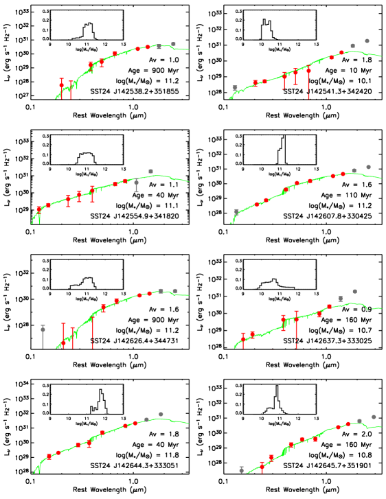
Figure 8.— Luminosity per unit frequency as a function of rest-frame wavelength for power-law DOGs (red circles). Gray circles indicate that $B_{W}$ and IRAC 5.8$\mu$m and 8.0$\mu$m data are not used to constrain the SPS models (see section 3.1). The best-fit CB07 synthesized stellar population (assuming a Chabrier IMF and a simple stellar population SFH) is shown in green with the best-fit parameters printed in the bottom right of each panel. The inset shows the stellar mass probability density function (marginalizing over model age and $A_{V}$) for each source.

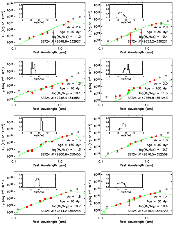
Figure 8.— Continued.

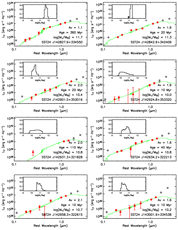
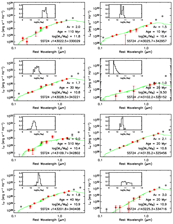
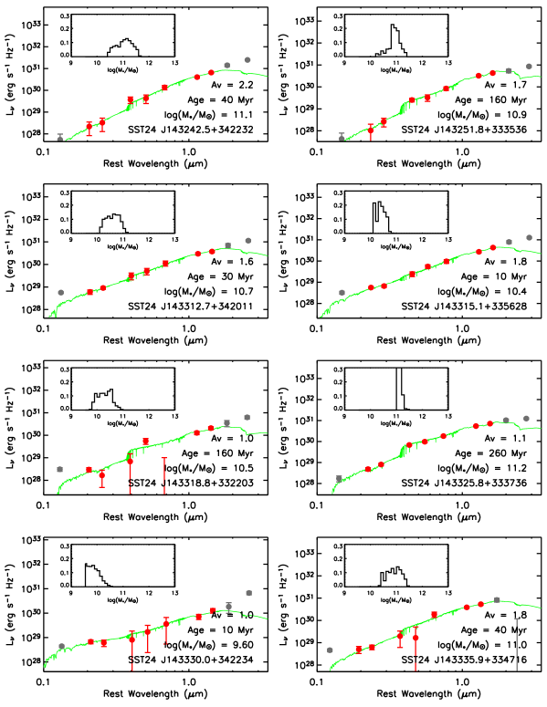
Figure 8.— Continued.

Figure 8.— Continued.

Figure 8.— Continued.

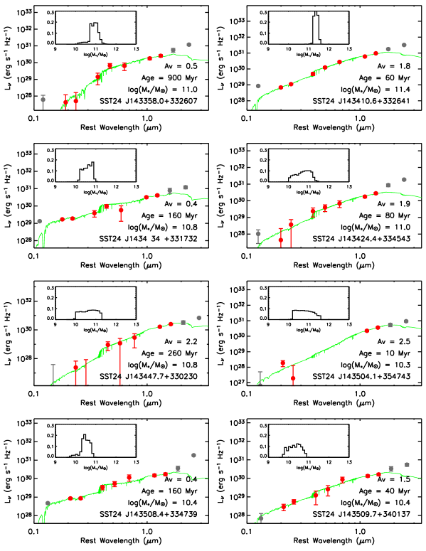
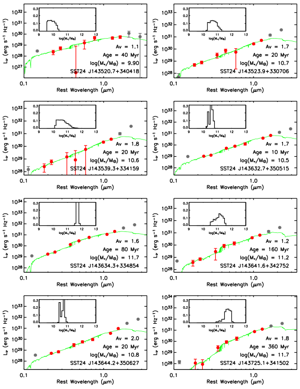
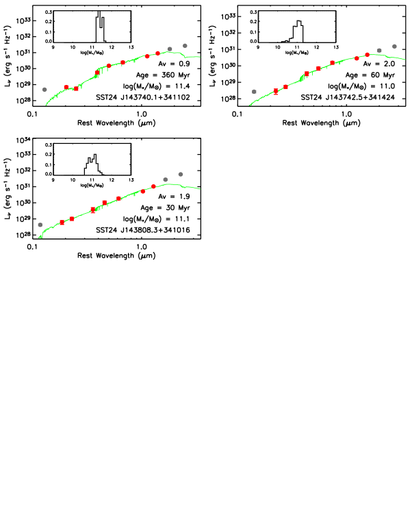
Figure 8.— Continued.

Figure 8.— Continued.

Figure 8.— Continued.

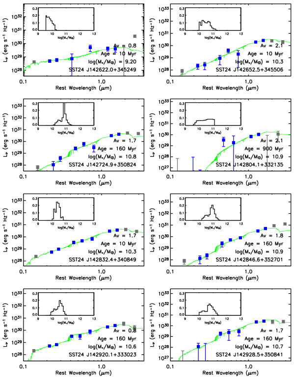
Figure 9.— Same as Figure 8, but for bump DOGs.

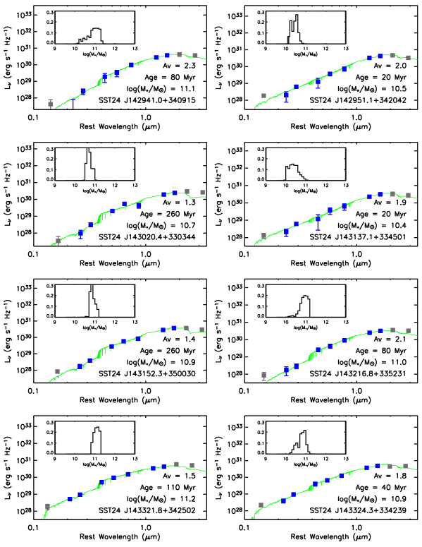
Figure 9.— Continued.

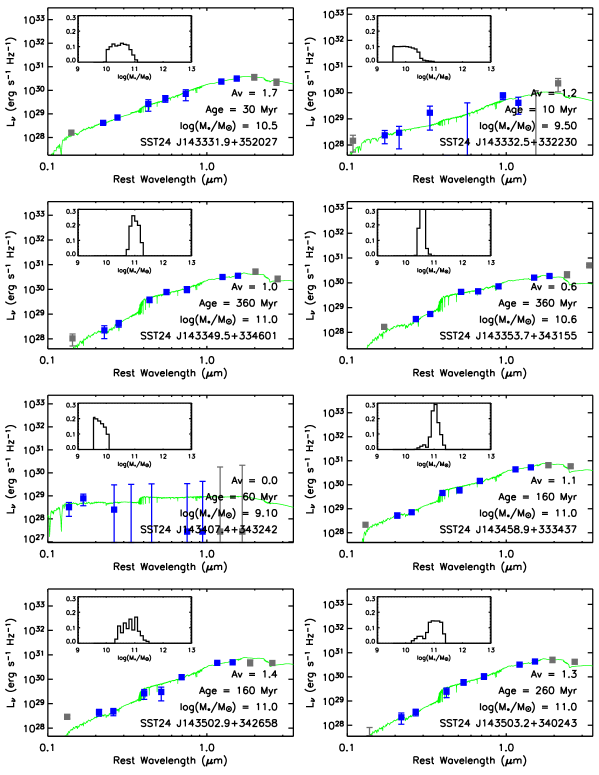
Figure 9.— Continued.

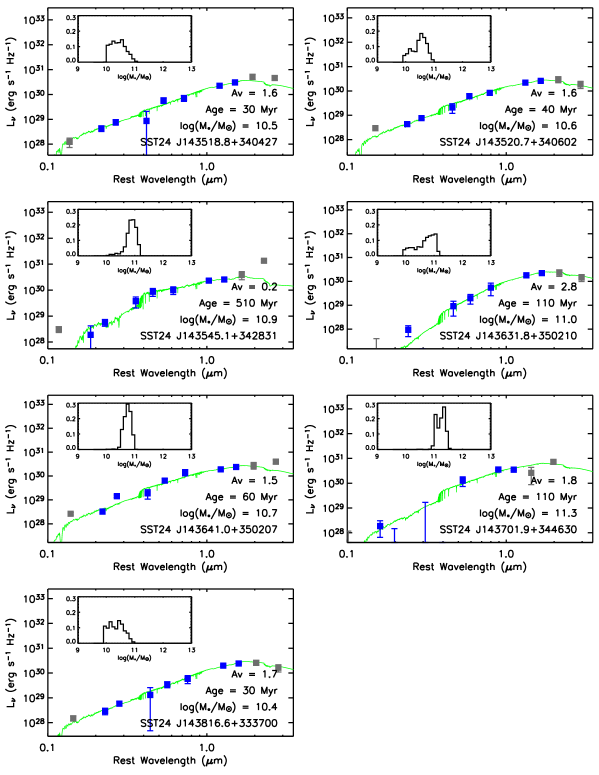
Figure 9.— Continued.

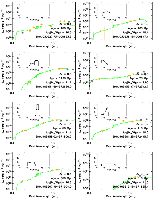
Figure 10.— Same as Figure 8, but for SMGs.

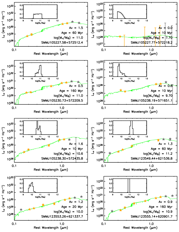
Figure 10.— Continued.

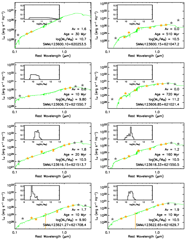
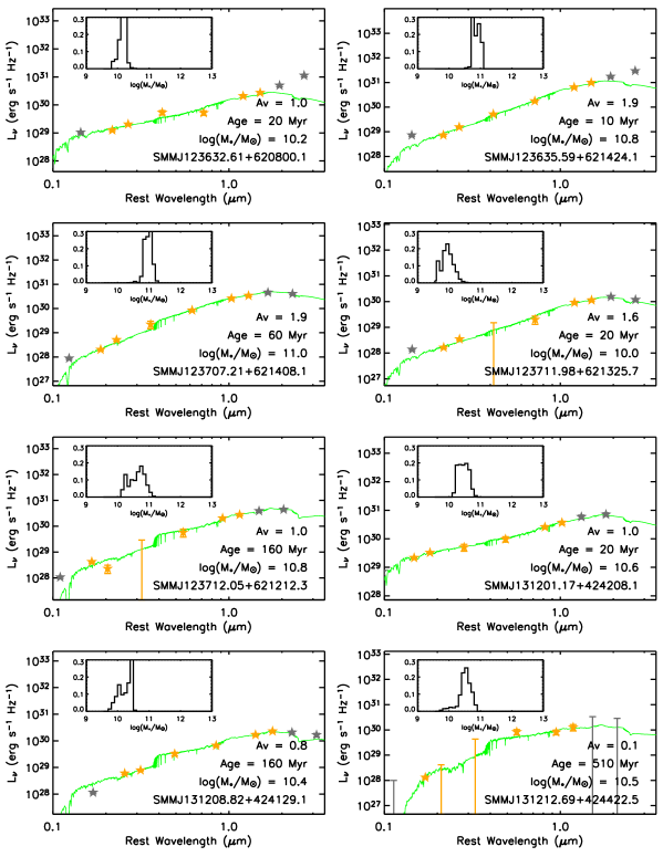
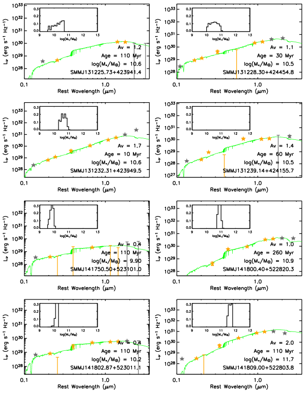
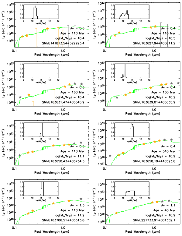
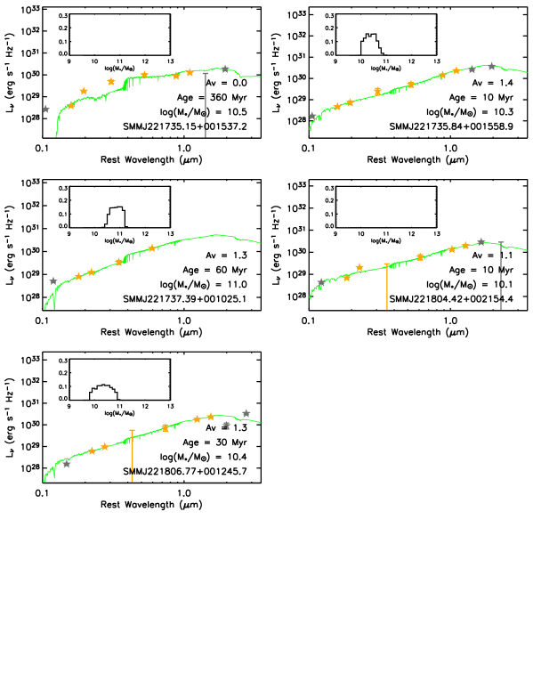
Figure 10.— Continued.

Figure 10.— Continued.

Figure 10.— Continued.

Figure 10.— Continued.

Figure 10.— Continued.

References

- Armus et al. (1987) Armus, L., Heckman, T., & Miley, G. 1987, AJ, 94, 831
- Ashby et al. (2009) Ashby, M. L. N. et al. 2009, ApJ, 701, 428
- Berta et al. (2007) Berta, S. et al. 2007, A&A, 476, 151
- Bertin & Arnouts (1996) Bertin, E. & Arnouts, S. 1996, A&AS, 117, 393
- Blain et al. (2004) Blain, A. W., Chapman, S. C., Smail, I., & Ivison, R. 2004, ApJ, 611, 725
- Bohlin et al. (1978) Bohlin, R. C., Savage, B. D., & Drake, J. F. 1978, ApJ, 224, 132
- Borys et al. (2005) Borys, C., Smail, I., Chapman, S. C., Blain, A. W., Alexander, D. M., & Ivison, R. J. 2005, ApJ, 635, 853
- Brand et al. (2007) Brand, K. et al. 2007, ApJ, 663, 204
- Brodwin et al. (2008) Brodwin, M., Dey, A., Brown, M. J. I., Pope, A., Armus, L., Bussmann, S., Desai, V., Jannuzi, B. T., & Le Floc’h, E. 2008, ApJ, 687, L65
- Bruzual & Charlot (2003) Bruzual, G. & Charlot, S. 2003, MNRAS, 344, 1000
- Bussmann et al. (2009a) Bussmann, R. S. et al. 2009a, ApJ, 693, 750
- Bussmann et al. (2009b) —. 2009b, ApJ, 705, 184
- Bussmann et al. (2011) —. 2011, ApJ, 733, 21
- Calzetti et al. (2000) Calzetti, D., Armus, L., Bohlin, R. C., Kinney, A. L., Koornneef, J., & Storchi-Bergmann, T. 2000, ApJ, 533, 682
- Chabrier (2003) Chabrier, G. 2003, PASP, 115, 763
- Chapman et al. (2005) Chapman, S. C., Blain, A. W., Smail, I., & Ivison, R. J. 2005, ApJ, 622, 772
- Charlot & Bruzual (1991) Charlot, S. & Bruzual, A. G. 1991, ApJ, 367, 126
- Charlot & Fall (2000) Charlot, S. & Fall, S. M. 2000, ApJ, 539, 718
- Conroy & Gunn (2010) Conroy, C. & Gunn, J. E. 2010, ApJ, 712, 833
- Conroy et al. (2009) Conroy, C., Gunn, J. E., & White, M. 2009, ApJ, 699, 486
- Conroy et al. (2010) Conroy, C., White, M., & Gunn, J. E. 2010, ApJ, 708, 58
- Conselice et al. (2003) Conselice, C. J., Chapman, S. C., & Windhorst, R. A. 2003, ApJ, 596, L5
- Coppin et al. (2008) Coppin, K. et al. 2008, MNRAS, 384, 1597
- Dasyra et al. (2008) Dasyra, K. M., Yan, L., Helou, G., Surace, J., Sajina, A., & Colbert, J. 2008, ApJ, 680, 232
- Davé (2008) Davé, R. 2008, MNRAS, 385, 147
- Davé et al. (2010) Davé, R., Finlator, K., Oppenheimer, B. D., Fardal, M., Katz, N., Kereš, D., & Weinberg, D. H. 2010, MNRAS, 404, 1355
- Desai et al. (2009) Desai, V. et al. 2009, ApJ, 700, 1190
- Dey & The NDWFS/MIPS Collaboration (2009) Dey, A. & The NDWFS/MIPS Collaboration. 2009, in Astronomical Society of the Pacific Conference Series, Vol. 408, Astronomical Society of the Pacific Conference Series, ed. W. Wang, Z. Yang, Z. Luo, & Z. Chen, 411–+
- Dey et al. (2008) Dey, A. et al. 2008, ApJ, 677, 943
- Donley et al. (2010) Donley, J. L., Rieke, G. H., Alexander, D. M., Egami, E., & Pérez-González, P. G. 2010, ApJ, 719, 1393
- Draine (2003) Draine, B. T. 2003, ARA&A, 41, 241
- Dye et al. (2008) Dye, S. et al. 2008, MNRAS, 386, 1107
- Eisenhardt et al. (2004) Eisenhardt, P. R. et al. 2004, ApJS, 154, 48
- Engel et al. (2010) Engel, H., Tacconi, L. J., Davies, R. I., Neri, R., Smail, I., Chapman, S. C., Genzel, R., Cox, P., Greve, T. R., Ivison, R. J., Blain, A., Bertoldi, F., & Omont, A. 2010, ApJ, 724, 233
- Farrah et al. (2008) Farrah, D., Lonsdale, C. J., Weedman, D. W., Spoon, H. W. W., Rowan-Robinson, M., Polletta, M., Oliver, S., Houck, J. R., & Smith, H. E. 2008, ApJ, 677, 957
- Fazio et al. (2004) Fazio, G. G. et al. 2004, ApJS, 154, 10
- Fiolet et al. (2009) Fiolet, N. et al. 2009, A&A, 508, 117
- Fiore et al. (2008) Fiore, F. et al. 2008, ApJ, 672, 94
- Fiore et al. (2009) —. 2009, ApJ, 693, 447
- Franceschini et al. (2001) Franceschini, A., Aussel, H., Cesarsky, C. J., Elbaz, D., & Fadda, D. 2001, A&A, 378, 1
- Girardi et al. (1996) Girardi, L., Bressan, A., Chiosi, C., Bertelli, G., & Nasi, E. 1996, A&AS, 117, 113
- Hainline et al. (2011) Hainline, L. J., Blain, A. W., Smail, I., Alexander, D. M., Armus, L., Chapman, S. C., & Ivison, R. J. 2011, ApJ, 740, 96
- Hainline et al. (2009) Hainline, L. J., Blain, A. W., Smail, I., Frayer, D. T., Chapman, S. C., Ivison, R. J., & Alexander, D. M. 2009, ApJ, 699, 1610
- Holland et al. (1999) Holland, W. S. et al. 1999, MNRAS, 303, 659
- Hopkins et al. (2006) Hopkins, P. F., Hernquist, L., Cox, T. J., Di Matteo, T., Robertson, B., & Springel, V. 2006, ApJS, 163, 1
- Houck et al. (2004) Houck, J. R. et al. 2004, ApJS, 154, 18
- Houck et al. (2005) —. 2005, ApJ, 622, L105
- Huang et al. (2009) Huang, J. et al. 2009, ApJ, 700, 183
- Iglesias-Páramo et al. (2007) Iglesias-Páramo, J. et al. 2007, ApJ, 670, 279
- Jannuzi & Dey (1999) Jannuzi, B. T. & Dey, A. 1999, in Astronomical Society of the Pacific Conference Series, Vol. 191, Photometric Redshifts and the Detection of High Redshift Galaxies, ed. R. Weymann, L. Storrie-Lombardi, M. Sawicki, & R. Brunner, 111–+
- Kovács et al. (2006) Kovács, A., Chapman, S. C., Dowell, C. D., Blain, A. W., Ivison, R. J., Smail, I., & Phillips, T. G. 2006, ApJ, 650, 592
- Kovács et al. (2010) Kovács, A. et al. 2010, ApJ, 717, 29
- Lançon & Mouhcine (2002) Lançon, A. & Mouhcine, M. 2002, A&A, 393, 167
- Lançon & Wood (2000) Lançon, A. & Wood, P. R. 2000, A&AS, 146, 217
- Le Borgne et al. (2003) Le Borgne, J., Bruzual, G., Pelló, R., Lançon, A., Rocca-Volmerange, B., Sanahuja, B., Schaerer, D., Soubiran, C., & Vílchez-Gómez, R. 2003, A&A, 402, 433
- Le Floc’h et al. (2005) Le Floc’h, E. et al. 2005, ApJ, 632, 169
- Lonsdale et al. (2009) Lonsdale, C. J. et al. 2009, ApJ, 692, 422
- Maraston (2005) Maraston, C. 2005, MNRAS, 362, 799
- Maraston et al. (2006) Maraston, C., Daddi, E., Renzini, A., Cimatti, A., Dickinson, M., Papovich, C., Pasquali, A., & Pirzkal, N. 2006, ApJ, 652, 85
- Marigo & Girardi (2007) Marigo, P. & Girardi, L. 2007, A&A, 469, 239
- Marigo et al. (2008) Marigo, P., Girardi, L., Bressan, A., Groenewegen, M. A. T., Silva, L., & Granato, G. L. 2008, A&A, 482, 883
- Melbourne et al. (2008) Melbourne, J. et al. 2008, AJ, 136, 1110
- Melbourne et al. (2009) —. 2009, AJ, 137, 4854
- Melbourne et al. (2011) —. 2011, AJ, 141, 141
- Michałowski et al. (2010) Michałowski, M., Hjorth, J., & Watson, D. 2010, A&A, 514, A67+
- Michałowski et al. (2011) Michałowski, M. J., Dunlop, J. S., Cirasuolo, M., Hjorth, J., Hayward, C. C., & Watson, D. 2011, ArXiv e-prints
- Mihos & Hernquist (1996) Mihos, J. C. & Hernquist, L. 1996, ApJ, 464, 641
- Murphy et al. (1996) Murphy, Jr., T. W., Armus, L., Matthews, K., Soifer, B. T., Mazzarella, J. M., Shupe, D. L., Strauss, M. A., & Neugebauer, G. 1996, AJ, 111, 1025
- Muzzin et al. (2009) Muzzin, A., Marchesini, D., van Dokkum, P. G., Labbé, I., Kriek, M., & Franx, M. 2009, ApJ, 701, 1839
- Narayanan et al. (2010) Narayanan, D. et al. 2010, MNRAS, 407, 1701
- Pérez-González et al. (2005) Pérez-González, P. G. et al. 2005, ApJ, 630, 82
- Rieke (1978) Rieke, G. H. 1978, ApJ, 226, 550
- Rieke et al. (2004) Rieke, G. H. et al. 2004, ApJS, 154, 25
- Sajina et al. (2007) Sajina, A., Yan, L., Armus, L., Choi, P., Fadda, D., Helou, G., & Spoon, H. 2007, ApJ, 664, 713
- Sajina et al. (2008) Sajina, A. et al. 2008, ApJ, 683, 659
- Salpeter (1955) Salpeter, E. E. 1955, ApJ, 121, 161
- Sanders et al. (1988a) Sanders, D. B., Soifer, B. T., Elias, J. H., Madore, B. F., Matthews, K., Neugebauer, G., & Scoville, N. Z. 1988a, ApJ, 325, 74
- Sanders et al. (1988b) Sanders, D. B., Soifer, B. T., Elias, J. H., Neugebauer, G., & Matthews, K. 1988b, ApJ, 328, L35
- Shen et al. (2009) Shen, Y. et al. 2009, ApJ, 697, 1656
- Smail et al. (2004) Smail, I., Chapman, S. C., Blain, A. W., & Ivison, R. J. 2004, ApJ, 616, 71
- Swinbank et al. (2004) Swinbank, A. M., Smail, I., Chapman, S. C., Blain, A. W., Ivison, R. J., & Keel, W. C. 2004, ApJ, 617, 64
- Swinbank et al. (2010) Swinbank, A. M. et al. 2010, MNRAS, 405, 234
- Tacconi et al. (2006) Tacconi, L. J. et al. 2006, ApJ, 640, 228
- Tacconi et al. (2008) —. 2008, ApJ, 680, 246
- van Dokkum (2008) van Dokkum, P. G. 2008, ApJ, 674, 29
- van Dokkum & Conroy (2010) van Dokkum, P. G. & Conroy, C. 2010, Nature, 468, 940
- van Dokkum et al. (2009) van Dokkum, P. G. et al. 2009, PASP, 121, 2
- Weedman et al. (2006a) Weedman, D. et al. 2006a, ApJ, 653, 101
- Weedman et al. (2006b) Weedman, D. W. et al. 2006b, ApJ, 651, 101
- Westera et al. (2002) Westera, P., Lejeune, T., Buser, R., Cuisinier, F., & Bruzual, G. 2002, A&A, 381, 524
- Yan et al. (2004) Yan, L. et al. 2004, ApJS, 154, 60
- Yan et al. (2007) —. 2007, ApJ, 658, 778
- Zamojski et al. (2011) Zamojski, M., Yan, L., Dasyra, K., Sajina, A., Surace, J., Heckman, T., & Helou, G. 2011, ApJ, 730, 125