An Excursion-Set Model for the Structure of GMCs and the ISM

Abstract

The ISM is governed by supersonic turbulence on a range of scales. We use this simple fact to develop a rigorous excursion-set model for the formation, structure, and time evolution of dense gas structures (e.g. GMCs, massive clumps and cores). Supersonic turbulence drives the density distribution in non-self gravitating regions to a lognormal with dispersion increasing with Mach number. We generalize this to include scales $\gtrsim h$ (the disk scale height), and use it to construct the statistical properties of the density field smoothed on a scale $R$. We then compare conditions for self-gravitating collapse including thermal, turbulent, and rotational (disk shear) support (reducing to the Jeans/Toomre criterion on small/large scales). We show that this becomes a well-defined barrier crossing problem. As such, an exact “bound object mass function” can be derived, from scales of the sonic length to well above the disk Jeans mass. This agrees remarkably well with observed GMC mass functions in the MW and other galaxies, with the only inputs being the total mass and size of the galaxies (to normalize the model). This explains the cutoff of the mass function and its power-law slope (close to, but slightly shallower than, $-2$). The model also predicts the linewidth-size and size-mass relations of clouds and the dependence of residuals from these relations on mean surface density/pressure, in excellent agreement with observations. We use this to predict the spatial correlation function/clustering of clouds and, by extension, star clusters; these also agree well with observations. We predict the size/mass function of “bubbles” or “holes” in the ISM, and show this can account for the observed HI hole distribution without requiring any local feedback/heating sources. We generalize the model to construct time-dependent “merger/fragmentation trees” which can be used to follow cloud evolution and construct semi-analytic models for the ISM, GMCs, and star-forming populations. We provide explicit recipes to construct these trees. We use a simple example to show that, if clouds are not destroyed in $\sim 1-5$ crossing times, then all the ISM mass would be trapped in collapsing objects even if the large-scale turbulent cascade were maintained.

1 Introduction

The origins and nature of structure in the interstellar medium (ISM) and giant molecular clouds (GMCs) represents one of the most important unresolved topics in both the study of star formation and galaxy formation. In recent years, there have been several major advances in our understanding of the relevant processes. It is clear that a large fraction of the mass in the ISM is supersonically turbulent over a wide range of scales, from the sonic length ($\sim 0.1\,$pc) through and above the disk scale height ($\sim$kpc). A generic consequence of this super-sonic turbulence – so long as it can be maintained – is that the density distribution converges towards a lognormal PDF, with a dispersion that scales weakly with mach number (e.g. Vazquez-Semadeni, 1994; Padoan et al., 1997; Scalo et al., 1998; Ostriker et al., 1999).

Without continuous energy injection, this turbulence would dissipate in a single crossing time, and the processes that “pump” turbulence (generally assumed to be related to feedback from massive stars) remain poorly understood (see e.g. Mac Low & Klessen, 2004; McKee & Ostriker, 2007; Hopkins et al., 2012, and references therein). However, provided this turbulence can be maintained, it is able to explain the relatively small fraction of mass which collapses under the runaway effects of self-gravity and cooling (Vázquez-Semadeni et al., 2003; Li et al., 2004; Li & Nakamura, 2006; Padoan & Nordlund, 2011). In this picture, star formation occurs within dense cores, themselves typically embedded inside giant molecular clouds (GMCs), which represent regions where turbulent density fluctuations become sufficiently overdense so as to be marginally self-gravitating and collapse (Evans, 1999; Gao & Solomon, 2004; Bussmann et al., 2008). Some other process such as stellar feedback is believed to be responsible for disrupting the clouds, after a few crossing times (e.g. Evans et al., 2009). The turbulent cascade has also been invoked to explain GMC scaling relations, such as the size-mass and linewidth-size relations (Larson, 1981; Scoville et al., 1987).

However, despite this progress, there remains no rigorous analytic theory that can simultaneously predict these properties, as well as other key observables such as the GMC mass function, and the spatial distribution of gas over and under-densities in the ISM.

The approximately Gaussian distribution of the logarithmic density field, though, suggests that considerable progress might be made by adapting the excursion set or “extended Press-Schechter” formalism. This has proven to be an extremely powerful tool in the study of cosmology and galaxy evolution. The seminal work by Press & Schechter (1974) derived the form of the halo mass function via a simple (albeit somewhat ad hoc) calculation of the mass fraction expected to be above a given threshold for collapse, expected in a Gaussian overdensity distribution with the variance as a function of scale derived from the density power spectrum. Bond et al. (1991) developed a rigorous analytic (and statistical Monte Carlo) formulation of this, defining the excursion set formalism for dark matter halos. Famously, this resolved the “cloud in cloud” problem, providing a means to calculate whether structures were embedded in larger collapsing regions. Since then, excursion set models of dark matter have been studied extensively: they have been generalized and used to predict – in addition to the halo mass function – the spatial distribution/correlation function of halos (Mo & White, 1996), the distribution of voids (Sheth & van de Weygaert, 2004), the evolution and structure of HII regions in re-ionization (Haiman et al., 2000; Furlanetto et al., 2004), and many higher-order properties used as cosmological probes. By incorporating the time-dependence of the field, they have been used to study the growth and merger histories of halos and to construct Monte Carlo “merger trees” (Bower, 1991; Lacey & Cole, 1993). These trees formed the basis for the extensive field of semi-analytic models for galaxy formation, in which analytic physical prescriptions for galaxy evolution are “painted onto” the background halo evolution (e.g. Somerville & Kolatt, 1999; Cole et al., 2000). It is not an exaggeration to say that it has proven to be one of the most powerful theoretical tools in the study of large scale structure and galaxy formation.

There have been other, growing suggestions of similarities between the mathematical structure of the ISM and that invoked in excursion set theory. The mass function of GMCs, for example, has a faint-end slope quite similar to that of galaxy halos (both close to ${\rm d}n/{\rm d}M\propto M^{-2}$), suggestive of hierarchical collapse. Vazquez-Semadeni (1994) attempted to rigorously examine whether the structure of the ISM should be “hierarchical,” although they strictly define this as the probability of many independent fluctuations dominating the “peaks” in the density distribution (which does not technically need to be satisfied in excursion set theory). This is related to (but not equivalent to) the large body of work on the quasi-fractal structure of the ISM (see e.g. Elmegreen, 2002, and references therein). On smaller scales, Krumholz & McKee (2005) suggested that the fraction of a lognormal PDF above a “collapse threshold” at the sonic length could explain the fractional mass forming stars per free-fall time, inside of GMCs. Padoan et al. (1997); Padoan & Nordlund (2002) suggested that the distribution of lognormal density fluctuations above a threshold overdensity could explain the shape of the stellar initial mass function (IMF). Scalo et al. (1998) explicitly discuss the analogy between this and cosmological density fluctuations, and Hennebelle & Chabrier (2008) expanded upon the Padoan et al. (1997) argument using a derivation almost exactly analogous to the original Press & Schechter (1974) derivation, and showed that it agreed well with the standard IMF.

But despite these suggestions, and the enormous successes of the excursion set model in cosmological applications, there has been no attempt to translate the excursion set formalism to the problem of the ISM and GMC evolution. At first glance, it is obvious why. The cosmological excursion set theory is applied to small fluctuations of the linear density field, in the linear regime, to dark matter (collisionless) systems, with Gaussian, nearly scale-free fluctuations seeded by inflation, and to Lagrangian “halos” which (modulo mergers) are conserved in time. The Gaussian distribution of ISM densities represent large fluctuations in the logarithmic density field, which are a product of a fully non-linear, turbulent, gaseous (collisional) medium, and evolve both rapidly and stochastically in time.

However, in this paper, we will show that although the physics involved are very different, none of these differences fundamentally invalidates the underlying mathematical formalism of the excursion set theory.

Here, we develop a rigorous excursion-set model for the formation, structure, and time evolution of structures in the ISM and within GMCs. We show that this is possible, and that it allows us to develop statistical predictions of ISM properties in a manner analogous to the predictions for the halo mass function. In § 2 we describe the model. First (§ 2.1), we derive the conditions for self-gravitating collapse in a turbulent medium (the “collapse threshold”), in a manner generalized to both small (sonic length) and large (above the disk scale height) scales. Next (§ 2.2), we discuss the density field, and, assuming it has a lognormal character, construct the statistical properties of the field smoothed on a physical scale $R$, which allows us to define the excursion set “barrier crossing” problem. In § 3, we use this to derive an exact “self-gravitating object” mass function, over the entire range of masses (from the sonic length to disk mass), and show that it agrees remarkably well with observed GMC mass functions and depends only very weakly on the exact turbulent properties of the medium (including deviations from a lognormal PDF). In § 4, we show that the model also predicts the linewidth-size and size-mass relations of GMCs, and their dependence on external galaxy properties. We also examine how this depends on the exact properties of the turbulent cascade. In § 5, we extend the model to predict the spatial correlation function and clustering properties of clouds (and, by extension, young star clusters), and compare this to observations. In § 6, we predict the size and mass distributions of underdense “bubbles” or “holes” in the ISM which result simply from the same normal turbulent motions. We show that this can explain most or all of the distribution of HI “holes” observed in nearby galaxies, without explicitly requiring any feedback mechanism to power the hole expansion. In § 7, we generalize the model to construct time-dependent “GMC merger/fragmentation trees” which follow the time evolution, growth histories, fragmentation, and mergers of clouds. In § 7.2 we provide simple recipes to construct these trees, and discuss how they can be used to build semi-analytic models for GMC and ISM evolution and star formation, in direct analogy to semi-analytic models for galaxy formation. We use a very simple example of this to predict the rate at which the gas in the ISM collapses (absent feedback) into bound structures, show that this agrees well with the results of fully non-linear turbulent box simulations, and argue that feedback must destroy clouds on a short timescale (a few crossing times) to prevent runaway gas consumption. Finally, in § 8, we summarize our results and conclusions and discuss a number of possibilities for future work, both to improve the accuracy of these models and to enable predictions for additional properties of the ISM.

2 The Model

The fundamental assumption of our model is that non-rotational velocities are dominated by super-sonic turbulence (down to some sonic length), with some power spectrum $P(k)$ or $E(k)$ which is maintained by any process (presumably stellar feedback) in approximate statistical steady-state. As we discuss in § 8, all other assumptions we make are convenient approximations to simplify our calculations, but it is possible to generalize the model.

The two key quantities we need to calculate the cloud mass function and other properties are the conditions for “collapse” of a cloud (i.e. conditions under which self-gravity can overcome turbulent forcing) and the power spectrum of density fluctuations. Below, we show how these can be calculated for a turbulent medium from the velocity power spectrum; however, in principle they can be completely arbitrary (for example, specified ad hoc from numerical simulations or observations). So long as they are known, the rest of our model proceeds identically.

2.1 Collapse in a Turbulent Medium

First, for simplicity, consider gas in a galaxy whose average properties are evaluated on a scale $R$ where the velocity dispersion is highly supersonic ($R\gg\ell_{\rm sonic}$, where $\ell_{\rm sonic}$ is the sonic length), but where shear from the disk rotation and large-scale density gradients can be neglected ($R\ll h$, where $h$ is the disk scale-height). The turbulent dispersion on these scales is $\langle v_{t}(R)^{2}\rangle\sim k\,E(k)$. If the turbulence has a power-law cascade over this interval then $E(k)\propto k^{-p}$. If the region has some mean density $\rho$ (on the same scale $R$), then the potential from self-gravity is $|U|\approx\beta\,GM/R\approx\beta G\rho(4\pi/3)\,R^{2}$ while the kinetic energy in turbulence is $(1/2)\,\langle v_{t}(R)^{2}\rangle$; the region will be gravitationally bound and “trapped” when $\rho\gtrsim\rho_{c}=(3/8\pi\beta)\,\langle v_{t}(R)^{2}\rangle/G\,R^{2}$, where $\beta\sim 1$ depends on the shape (internal structure) of the density perturbation. Formally, we also need to check whether the momentum “input” rate from the turbulent cascade (equal to the dissipation rate in steady-state) is less than the gravitational force, and whether the energy input rate is less than the rate at which a gravitationally collapsing object will dissipate. However, because for super-sonic turbulence, the timescale for energy or momentum dissipation on a scale $R$ just scales with the crossing time $t_{\rm cross}=R/v_{t}(R)$, we obtain the identical dimensional scaling for all of these criteria.

These are simply a restatement of the Jeans criterion, for wavenumber $k\sim 1/R$, but with the sound speed $c_{s}$ replaced by the turbulent velocity dispersion $v_{t}$. For an individual $k$-mode (sinusoidal density perturbation), the criteria becomes

$$\rho(R)\geq\frac{k^{2}\langle v_{t}^{2}(k)\rangle}{4\pi\,G}\propto k^{3-p}\propto R^{p-3}$$ (1)

where the latter equalities assume a power-law spectrum (Vazquez-Semadeni & Gazol, 1995). If the system is marginally stable with density $\rho_{0}$ on scale $R_{0}$, then this simply becomes $\rho(R)\geq\rho_{0}\,(R/R_{0})^{p-3}$. If we are in the super-sonic regime, then we expect something like Burgers turbulence (Burgers, 1973), with $p\approx 2$; but we will discuss this further below.

Now generalize this to a more broad range of radii. On small scales, we need to include the effects of thermal pressure: this amounts to a straightforward modification of the Jeans criterion with $v_{t}^{2}\rightarrow c_{s}^{2}+v_{t}^{2}$ (Chandrasekhar, 1951; Bonazzola et al., 1987). On large scales, we need to include the effects of rotation stabilizing perturbations. If we focused only on very large ($R\gg h$) scales, where we can neglect the disk thickness, then we simply re-derive the (Toomre, 1977) dispersion relation and collapse conditions, with the gas “dispersion” $\sigma_{g}^{2}=v_{t}^{2}+c_{s}^{2}$. More generally, Begelman & Shlosman (2009) note that the dispersion relation for growth of density perturbations in a turbulent disk (with finite thickness $h$) can be written:

$$\omega^{2} =\kappa^{2}+\sigma_{g}(k)^{2}\,k^{2}-\frac{2\pi\,G\,\Sigma\,|k|}{1+|k|\,h}$$ (2)

$$=\kappa^{2}+\sigma_{g}(k)^{2}\,k^{2}-\frac{4\pi\,G\,\rho\,|k|\,h}{1+|k|\,h}$$ (3)

where $\Sigma\equiv 2\,h\,\rho$ is the disk surface density, $\rho$ the average density on scale $k$, and $h$ the disk scale-height, $v_{t}$ the turbulent velocity dispersion, and $\kappa$ the usual epicyclic frequency. This differs from the infinitely thin-disk dispersion relation by the term $(1+|k|\,h)^{-1}$, which accounts for the finite scale height for modes with scales $\lambda\lesssim h$ (Vandervoort, 1970; Elmegreen, 1987; Romeo, 1992). Note that this relation nicely interpolates between the Jeans criterion which we derived above on small scales ($k\gg h^{-1}$), and the Toomre (thin-disk) dispersion relation on large scales ($k\ll h^{-1}$).

If the average density is $\rho_{0}$, and corresponding average surface density $\Sigma_{0}$, then we can define the usual Toomre $Q$ at the scale $h$

$$Q_{0}(h)\equiv\frac{\kappa\,\sigma_{g}(h)}{\pi\,G\,\Sigma_{0}}=\frac{h\,\tilde{\kappa}\,\Omega^{2}}{\pi\,G\,\Sigma_{0}}$$ (4)

where the second equality follows from $\sigma_{g}(h)=h\,\Omega$, which is be true for any disk in vertical equilibrium, and we define $\tilde{\kappa}\equiv\kappa/\Omega$ ($=\sqrt{2}$ for a constant-$V_{c}$ disk). If we define the convenient dimensionless form of $k$, $\tilde{k}\equiv|k|\,h$, we can write the criterion for instability ($\omega^{2}<0$) as

$$\frac{\rho}{\rho_{0}} \geq\frac{\rho_{c}}{\rho_{0}}\equiv\frac{Q_{0}(h)}{2\,\tilde{\kappa}}\,(1+\tilde{k}){\Bigl{[}}\frac{\sigma_{g}(k)^{2}}{\sigma_{g}(h)^{2}}\,\tilde{k}+\tilde{\kappa}^{2}\,\tilde{k}^{-1}{\Bigr{]}}$$ (5)

Note that the assumption of a finite $Q_{0}$ ensures that so long as there is any non-gaseous component of the potential, the gas alone is not self-gravitating on arbitrarily large scales (this is important below, to un-ambiguously define the largest self-gravitating scales of clouds). Again, on small scales $kh\gg 1$, this reduces to the Jeans criterion $\rho_{c}=k^{2}\,\sigma_{g}(k)^{2}/(4\pi\,G)\propto R^{p-3}$, and on large scales $kh\ll 1$ it becomes $\rho_{c}=\Sigma_{c}/2h=(k\,h)^{-1}\kappa^{2}/(4\pi G)\propto R$.

Kim et al. (2002) note that is straightforward to further generalize this criterion to include the effects of magnetic fields by taking $\sigma_{g}^{2}=v_{t}^{2}+c_{s}^{2}+v_{\rm A}^{2}$, where $v_{\rm A}^{2}$ is the Alfvèn speed. If we follow the usual convention in the literature and assume $\beta\equiv c_{s}^{2}/v_{\rm A}^{2}$ is constant, then changing the strength of magnetic fields is identically equivalent to changing the sound speed/mach number (which we explicitly consider below). Even if we allow $\beta$ to have an arbitrary power spectrum, the results are quite similar to this renormalization – for any power spectrum where the magnetic energy density is peaked on large scales, it is nearly equivalent to renormalizing the turbulent velocities; for a power spectrum peaked on small scales, equivalent to renormalizing the sound speed. We therefore will not explicitly consider magnetic fields in what follows, but emphasize that they are straightforward to include if their power spectrum is known.

Formally, the turbulent velocity power spectrum $E(k)$ must eventually flatten/turn over on large scales $R\gtrsim h$, both by definition (since $h$ itself traces the maximal three-dimensional dispersions) and to avoid energy divergences. If it did not, we would recover $v_{t}\gtrsim V_{c}$ on large scales in gas-rich systems! Constancy of energy transfer and energy conservation require that the slope become at least as shallow as $E(k)\propto k^{-1}$. A good approximation to the behavior seen in simulations is obtained by generalizing the exact correction for $k$ near the lowest wavenumbers in the inertial scale in Kolmogorov turbulence (Bowman, 1996), taking $E(k)\rightarrow E(k)\,(1+|k\,h|^{-2})^{(1-p)/2}$, which interpolates between these regimes. This may not be exact. Fortunately however, even if we ignored this correction entirely, we can see immediately from Equation 5 that for any reasonable power spectrum ($p<3$), the dominant velocity/pressure term on scales $\gtrsim h$ is the disk shear ($\sim\kappa\,R$), not $v_{t}$. We therefore include this turnover, but stress that it is not necessary to our derivation and has only weak effects on our conclusions.

2.2 The Density Distribution

The other required ingredient for our model is an estimate of the density PDF/power spectrum. We emphasize that the our methodology is robust to the choice of an arbitrary PDF and/or power spectrum in $\rho$. We could, for example, simply extract a density power spectrum (or fit to it) from simulations or observations. This is, however, less predictive – so in this paper, we chose to focus on the case of supersonic turbulence in which case it is possible to (at least approximately) construct the density PDF knowing only the velocity power spectrum information.

As discussed in § 1, in idealized simulations of supersonic turbulence with a well-defined mean density $\rho_{0}$ and mach number $\mathcal{M}$ on a scale $k\sim 1/R$, the distribution of densities tends towards a lognormal distribution

$${\rm d}p(\delta\,|\,k) =\frac{1}{\sigma_{k}\sqrt{2\pi}}\,\exp{{\Bigl{(}}-\frac{\delta^{2}}{2\,\sigma_{k}^{2}}{\Bigr{)}}}\,{\rm d}{\delta}$$ (6)

$$\delta \equiv\ln{{\Bigl{(}}\frac{\rho}{\rho_{0}}{\Bigr{)}}}-{\Bigl{\langle}}{\ln{{\Bigl{(}}\frac{\rho}{\rho_{0}}{\Bigr{)}}}}{\Bigr{\rangle}}$$ (7)

where because $\rho_{0}$ is the mean density,

$${\Bigl{\langle}}{\ln{{\Bigl{(}}\frac{\rho}{\rho_{0}}{\Bigr{)}}}}{\Bigr{\rangle}}=-\frac{\sigma_{k}^{2}}{2}$$ (8)

This form of the PDF and our results are identical whether we define all quantities as volume-weighted or mass-weighted, so long as we are consistent throughout: here it is convenient to define all properties as volume-weighted (otherwise $\rho_{0}$ is scale-dependent).

The dispersion in these simulations is a function of the rms (one-dimensional) Mach number averaged on the same scale $\mathcal{M}(k)$,

$$\sigma_{k}\approx{\Bigl{(}}\ln{{\Bigl{[}}1+\frac{3}{4}\,{\mathcal{M}(k)^{2}}{\Bigr{]}}}{\Bigr{)}}^{1/2}$$ (9)

which is naturally expected for supersonic turbulence with efficient cooling (because the variance in $\ln{(\rho)}$ in “events” – namely strong shocks – scales as $\ln{(\mathcal{M}^{2})}$).

If the turbulence obeys locality – i.e. if the density distribution averaged on some small scale $R_{1}$ depends only on the local gas properties on that scale as opposed to e.g. the structure on much larger scales $R_{2}\gg R_{1}$ – then the distribution of densities $\delta({\bf x},\,R)$ averaged over any spatial scale $R$ with some window function $W({\bf x},\,R)$ is also a lognormal in $\delta$, with variance

$$\sigma^{2}(R)=\int{\rm d}\ln{(k)}\,\sigma_{k}^{2}(\mathcal{M}[k])\,|W(k,\,R)|^{2}$$ (10)

where $W(k,\,R)$ is the Fourier transform of $W(x,\,R)$. This is easy to see if we recursively divide an initially large volume (e.g. the entire disk) into sub-regions with different mean $\rho_{0}$ and $\mathcal{M}$ on scale $R$; each of these sub-regions is a “box” that should obey the density distributions above, and so on. Because it greatly simplifies the algebra, we will generally follow the standard practice in the excursion set literature and choose $W(k,\,R)$ to be a Fourier-space top-hat: $W(k\,|\,R_{w})=1$ if $k\leq R_{w}^{-1}$ and $W(k\,|\,R_{w})=0$ if $k>R_{w}^{-1}$. This choice is arbitrary, but so long as it is treated consistently, our subsequent results are essentially identical (we will show, for example, that using a Gaussian window function makes a small difference in all predicted quantities).

It should immediately be clear, however, that if we simply extrapolated $\mathcal{M}^{2}=v_{t}^{2}/c_{s}^{2}\propto R^{(p-1)/2}$, the dispersion would be divergent! Physically, this would imply ever larger fluctuations in $\log{\rho}$ on arbitrarily large scales; but this cannot be true once the scale $R$ approaches that of the entire disk. As $kh\rightarrow 0$, the fact that the disk has finite mass means that $\sigma_{k}\rightarrow 0$. The resolution of this apparent dilemma is evident in Equation 2: what matters in $\mathcal{M}$ in the dispersion is the effective “pressure” from $c_{s}^{2}$; on sufficiently large scales $kh\ll 1$, the differential rotation $\kappa/k$ plays an identical physical role. We can therefore generalize Equation 9 as

$$\sigma_{k} \approx{\Bigl{(}}\ln{{\Bigl{[}}1+\frac{3}{4}\,\frac{v_{t}^{2}(k)}{c_{s}^{2}+\kappa^{2}\,k^{-2}}{\Bigr{]}}}{\Bigr{)}}^{1/2}$$ (11)

$$={\Bigl{(}}\ln{{\Bigl{[}}1+\frac{3}{4}\,\frac{\mathcal{M}^{2}(k)}{1+\mathcal{M}_{h}^{2}\tilde{\kappa}^{2}/|kh|^{2}}{\Bigr{]}}}{\Bigr{)}}^{1/2}$$ (12)

where $\mathcal{M}_{h}\equiv\sigma_{g}(h)/c_{s}$. This ensures the correct physical behavior, $\sigma_{k}\rightarrow 0$ as $k\rightarrow 0$ for all plausible turbulent $E(k)$.

At some level, our assumptions must break down. And although it is well-established that the density PDF at the resolution limit in numerical simulations (in a “box-averaged” sense) approaches the behavior of Eqns. 6-9, it is less clear whether we can assume this on a $k$-by-$k$ basis and so derive Eqns. 10-11. The lognormal character of the density distribution holding on various smoothing scales as we assume is, however, supported in the investigations of Lemaster & Stone (2009) and Passot & Vazquez-Semadeni (1998); Scalo et al. (1998). And any distribution which is lognormal in either real space or $k$ space must be lognormal in both. Moreover, the robustness of this assumption is supported by the conservation of lognormality in resolution studies, since all simulations essentially measure the PDF smoothed over a window function corresponding to their resolution limits. To the extent that there is some violation of these assumptions in e.g. the higher-order-structure functions (although they are largely consistent with locality when $\mathcal{M}_{h}$ is large; see Boldyrev et al., 2002; Padoan et al., 2004; Schmidt et al., 2008), this is really a question of the degree to which the density PDF globally departs from a lognormal, which we discuss below.

What is somewhat less clear is how Eq. 9 generalizes on a scale-by-scale basis. Analytically, the same arguments that prove the density distribution of isothermal turbulence should converge to a lognormal with real-space variance $\sigma^{2}=\ln{(1+(3/4)\langle\mathcal{M}^{2}\rangle)}$ trivially generalize to a $k$-by-$k$ basis (Eq. 9; see Passot & Vazquez-Semadeni, 1998; Nordlund & Padoan, 1999). If locality also holds, Eq. 10 must follow. This is the origin of the expectation for analytic models of the density power spectrum. Note that, as defined, $\sigma_{k}^{2}$ is equivalent to the logarithmic density power spectrum, $\sigma_{k}^{2}=k\,E_{\ln{\rho}}(k)$. When $\mathcal{M}$ is not large, $\sigma_{k}^{2}$ in Eq. 9 scales $\propto\mathcal{M}(k)^{2}\propto v_{t}^{2}\sim k\,E(k)$, so $E_{\ln{\rho}}(k)\propto E(k)$. This is just the well-known expectation that in the weakly compressible regime, the log density power spectrum should have the same shape as the velocity power spectrum. Kowal et al. (2007) and Schmidt et al. (2009) show that this is a good approximation for the $\ln{(\rho)}$ field in simulations of supersonic turbulence. At higher $\mathcal{M}$, this should flatten logarithmically, and this is seen in numerical simulations in Kowal et al. (2007), in excellent agreement with Eq. 9. These behaviors, and the approximate normality of $\ln{(\rho)}$, appear to hold even in simulations which include explicitly non-local effects such as magnetic fields, self-gravity (excluding the collapsing regions), radiation pressure, photoionization, and non-isothermal gas with realistic heating/cooling (see e.g. Ostriker et al., 1999; Klessen, 2000; Lemaster & Stone, 2009; Hopkins et al., 2012).

Even if our analytic derivation is not exact, we can think of the resulting $\sigma^{2}(R)$ and implied log density power spectrum ($E_{\ln{\rho}}(k)\sim k^{-1}\sigma^{2}_{k}$) as a convenient approximation for the power spectrum measured in hydrodynamic simulations and observations. At sufficiently large $k$, where $\mathcal{M}$ is small, $E_{\ln{\rho}}(k)\propto k^{-1}\mathcal{M}^{2}\propto k^{-p}$; a steep falloff with $k$ for typical $p\approx 2$; at smaller $k$ (but still smaller scales than the disk scale-height) $\mathcal{M}$ is large and this flattens to $E_{\ln{\rho}}(k)\propto k^{-1}\ln{\mathcal{M}^{2}}\propto k^{-1}$ with a small logarithmic correction. This is exactly the behavior directly measured in numerical simulations (Kowal et al., 2007; Schmidt et al., 2009). Qualitatively similar behavior is seen in the linear density spectrum, but it is important to distinguish the two, since it is well known that large fluctuations at higher $\mathcal{M}$ will further flatten the linear spectrum (see Scalo et al., 1998; Vázquez-Semadeni & García, 2001; Kim & Ryu, 2005; Kritsuk et al., 2007; Bournaud et al., 2010). It is also consistent with observations of the projected surface density power spectrum in local galaxies and star-forming regions (Stanimirovic et al., 1999; Padoan et al., 2006; Block et al., 2010). If we integrate to get $\sigma(R)$ we obtain $\sigma\rightarrow$constant as $R\rightarrow 0$, with an absolute value of $\sigma(R)\approx 1.25-1.9$ dex for a range $p=5/3-2$ and $\mathcal{M}_{h}=10-50$. This range is quite similar to the range measured in $\sigma(R)$ on the smallest resolved scales in a wide range of simulations that have a sufficiently large dynamic range in scales to probe the typical Mach numbers in GMCs and disk scale heights (see Vazquez-Semadeni, 1994; Nordlund & Padoan, 1999; Ostriker et al., 2001; Mac Low & Klessen, 2004; Slyz et al., 2005; Hopkins et al., 2012). It also agrees well with measured values of the dispersion in the real ISM (Wong et al., 2008; Goodman et al., 2009a; Federrath et al., 2010).

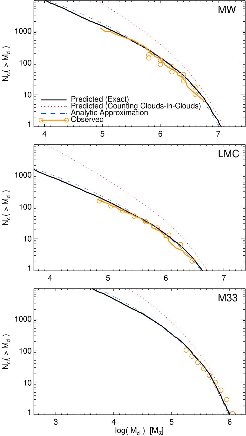
Figure 1: Predicted & observed (orange) GMC mass functions. The generally predicted mass function is dimensionless; we normalize it to the observed surface density $\Sigma_{\rm gas}$, gas density (or scale height) $n_{0}$, and total gas mass $M_{\rm gas}$. Together with the assumption that $Q\sim 1$, this completely specifies the model. For each case, we show the exact (Monte Carlo) mass function (solid black), and the mass function if we ignore the “cloud in cloud” problem by counting bound mass on all scales (dotted red); and the analytic fit to the mass function in Eq. 23 (dashed blue). Top: Milky Way. The observed MFs are taken from Williams & McKee (1997) (solid line) and Rosolowsky (2005) (orange points in each panel), & model normalized to $(\Sigma_{\rm gas},\,n_{0},\,M_{\rm gas})=(10\,M_{\sun}\,{\rm pc^{-2}},\,1\,{\rm cm^{-3}},\,3\times 10^{9}\,M_{\sun})$. Middle: LMC. Observed MF from Fukui et al. (2008) (line), normalized to $(8\,M_{\sun}\,{\rm pc^{-2}},\,0.8\,{\rm cm^{-3}},\,3\times 10^{8}\,M_{\sun})$ (see Wong et al., 2009). Bottom: M33. Normalized to $(5\,M_{\sun}\,{\rm pc^{-2}},\,1.5\,{\rm cm^{-3}},\,1\times 10^{9}\,M_{\sun})$ (see Engargiola et al., 2003).

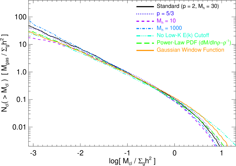
Figure 2: Variation in the predicted GMC mass function with model assumptions. The MFs are plotted in dimensionless units. We compare the standard model (from Fig. 1), which assumes a turbulent spectral index $p=2$, and Mach number at scale $\sim h$ of $\mathcal{M}_{h}=30$. Assuming $p=5/3$ instead slightly flattens the slope at intermediate masses. Changing $\mathcal{M}_{h}=10,\,1000$ increases/decreases the sonic length, below which the MF flattens, but near the MF break, the assumption of $Q\sim 1$ means that $\mathcal{M}_{h}$ factors out. Removing the assumed cutoff in the turbulent power spectrum at scales $\gg h$ makes the cutoff in the MF shallower at large masses. Using a Gaussian window function to smooth the density field (instead of the usual $k$-space tophat) makes the MF slightly more shallow, because for the same window volume (same mass definition), the radii which contribute fluctuations are shifted. In all these models, the density PDF is assumed to be lognormal; if we instead assume it is a pure power-law distribution (Eq. 34), but assume the same variance in $\ln{\rho}$, the result is nearly identical. In all cases, the variations in the MF are very small – the marginal stability assumption, and weak (logarithmic) running of density variance with scale mean the MF shape is largely independent of even substantial model assumptions.

3 The Mass Function

The question of the mass collapsed on different scales is now a well-posed barrier crossing problem. The quantity $\delta(R)$ – the logarithm of the density smoothed on the scale $R$ – is distributed as a Gaussian random field with variance $\sigma^{2}(R)$ and zero mean, with a well-defined barrier

$$\delta_{c}(R)\equiv\delta(\rho_{c},\,R)=\ln{{\Bigl{(}}\frac{\rho_{c}}{\rho_{0}}{\Bigr{)}}}-{\Bigl{\langle}}{\ln{{\Bigl{(}}\frac{\rho}{\rho_{0}}{\Bigr{)}}}}{\Bigr{\rangle}}$$ (13)

which, upon crossing, leads to collapse. The mass of a collapsed object is simply the integral of the density over the effective volume of a window of effective radius $R_{w}$ in real space. If the medium were infinite and homogenous, this would just be $M(R_{w})\equiv(4\pi/3)\,\rho_{c}(R_{w})\,R_{w}^{3}$; however, we need to account for the finite vertical thickness of the disk. For the same vertical exponential profile that gives rise to the dispersion relation in Equation 2, the total mass inside $R_{w}$ is

$$M(\rho\,|\,R_{w})\equiv 4\,\pi\,\rho(R_{w})\,h^{3}\,{\Bigl{[}}\frac{R_{w}^{2}}{2\,h^{2}}+{\Bigl{(}}1+\frac{R_{w}}{h}{\Bigr{)}}\,\exp{{\Bigl{(}}-\frac{R_{w}}{h}{\Bigr{)}}}-1{\Bigr{]}}$$ (14)

where $\rho(R_{w})$ is the midplane density (chosen for consistency with the dispersion relation). This formula simply interpolates between $M=(4\pi/3)\,\rho\,R^{3}$ for $R\lesssim h$ and $M=\pi\,(2\rho\,h)\,R^{2}=\pi\,\Sigma\,R^{2}$ for $R\gtrsim h$, as it should.

The fraction of the total mass which is in collapsed objects, averaged over a given smoothing scale $R_{w}$, is then just

$$F_{\rm coll}(R_{w})=\frac{1}{M_{\rm tot}}\int_{\delta_{c}}^{\infty}\,M(\rho\,|\,R_{w})\,p(\delta\,|\,R_{w})\,{\rm d}\,\delta$$ (15)

where $\rho(\delta)=\rho_{0}\,\exp{(\delta-\sigma[R_{w}]^{2}/2)}$. Naively, we would equate this to the mass function of such objects with the relation $M_{\rm tot}\,{\rm d}\,F_{\rm coll}/{\rm d}\,M=M\,{\rm d}N(M)/{\rm d}M$. Indeed, up to a normalization factor, that is exactly the original approach of Press & Schechter (1974). However, this neglects the “cloud in cloud” problem: namely, it does not resolve whether or not a collapsed region on a scale $R_{1}$ is independent, or is simply a random sub-region of a larger object collapsed on a scale $R_{0}>R_{1}$. For the case of a constant $\delta_{c}$, accounting for this amounts to a simple re-normalization; but there is no simple closed-form analytic solution for the complicated $\delta_{c}$ here, and we will show that accounting for this behavior is critical.

3.1 Exact Solution

To derive the exact mass function solution we turn to the standard Monte Carlo excursion-set approach. Consider the density field at some arbitrary location ${\bf x}$, smoothed over some window corresponding to the radius $R$ (and mass $M$) $\delta({\bf x}\,|\,R_{w})$. This is the convolution $\delta{({\bf x}\,|\,R_{w})}\equiv\int{{\rm d}^{3}x^{\prime}\,W(|{\bf x}^{\prime}-{\bf x}|,\,R_{w})\,\delta{({\bf x}^{\prime})}}$; so if we Fourier transform, we obtain $\delta{({\bf k}\,|\,R_{w})}\equiv W({\bf k}\,|\,R_{w})\,\delta({\bf k})$. In other words, the amplitude $\delta{({\bf x}\,|\,R_{w})}$ is simply the integral of the contribution from all Fourier modes $\delta({\bf k})$, weighted by the Fourier-space window function.

In this sense, we can think of the (statistical) evaluation of the density field as the results of a “random walk” through Fourier space. Bond et al. (1991) show that this integration becomes particularly simple for the case of a Gaussian field with a Fourier-space tophat window, in which case the probability of a transition from $\delta_{1}$ to $\delta_{2}\equiv\delta_{1}+\Delta\delta$ as we step from a scale $k_{1}$ to $k_{2}$ is given by

$$p(\delta_{1}+\Delta\,\delta)\,{\rm d}\,\Delta\,\delta =\frac{1}{\sqrt{2\pi\,\Delta\,S}}\,\exp{{\Bigl{(}}-\frac{(\Delta\,\delta)^{2}}{2\,\Delta\,S}{\Bigr{)}}}{\rm d}(\Delta\,\delta)$$ (16)

$$\Delta\,S \equiv S_{2}-S_{1}\equiv\sigma^{2}(R_{2})-\sigma^{2}(R_{1})$$ (17)

where we define the variance

$$S(R)\equiv\sigma^{2}(R)$$ (18)

i.e. the increment $\Delta\,\delta$ is a Gaussian random variable with standard deviation $\sqrt{\Delta\,S}$.

If we begin on some sufficiently large initial scale $k\rightarrow 0$ ($R\rightarrow\infty$), then the overdensity $\delta$ and density variations $\sigma(R)$ must go to zero. We then have the well-defined initial conditions for the walk, $\delta(R_{\rm max}\rightarrow\infty)=0$, $S(R_{\rm max}\rightarrow\infty)=0$. Starting at some arbitrarily large $R_{\rm max}$, and moving to progressively smaller scales with increments in $R$ or $S$ ($\Delta\,R_{i}$ or $\Delta\,S_{i}$) we can then compute the trajectory $\delta(R)$ or $\delta(S)$,

$$\delta(R_{i})\equiv\sum_{j}^{R_{j}>R_{i}}\Delta\,\delta_{j}\ .$$ (19)

At each scale $R_{i}$, we then evaluate whether or not the barrier has been crossed,

$$\delta(R_{i})\geq\delta_{c}(R_{i})\ .$$ (20)

If this is satisfied, we then associate that trajectory with a collapse on the scale $R_{i}$ and mass $M(\rho_{c}[R_{i}]\,|\,R_{i})\equiv M(R_{i})$.

Recall, we are sampling the field $\delta({\bf x}\,|\,R_{w})$, so the fraction of trajectories that cross the barrier in some interval $\Delta R_{i}$ or (equivalently) $\Delta M(R_{i})$ represents the probability of an Eulerian volume element being collapsed on that scale. This corresponds to a differential mass $df_{\rm mass}=\rho(\delta\,|\,R_{w})\,df_{\rm vol}=\rho_{c}[R_{i}]\,df_{\rm Vol}$. Since the total mass associated with the mass function is $M_{\rm tot}\,{\rm d}N(M)/{\rm d}M$, we have the predicted mass function or “first-crossing distribution”:

$$\frac{{\rm d}n}{{\rm d}M}=\frac{\rho_{c}(M)}{M}\,\frac{{\rm d}f}{{\rm d}M}$$ (21)

where ${\rm d}f/{{\rm d}M}$ is the differential fraction of trajectories that cross $\delta_{c}$ between $M$ and $M+{\rm d}M$.

This formalism has several advantages. It provides an exact solution that also allows us to rigorously calculate the normalization and shape of the mass function. It also allows us to explicitly resolve the “cloud-in-cloud” problem, i.e. to address the situation where a trajectory crosses the barrier $\delta_{c}$ multiple times. Figure 1 plots the resulting mass function (for a few choices of parameters, which just determine the normalization of the mass function and will be discussed below). We also compare the mass function if we were to ignore the “cloud in cloud” problem – i.e. where we treat every crossing above $\rho_{c}$ on a smoothing scale $R$ as a separate cloud. At the highest masses, the difference is small – this is because the variance is small and $\delta_{c}$ is large, so the probability of being inside a “yet larger” cloud vanishes. However, at lower masses, the difference rapidly becomes quite large (order-of-magnitude) – much larger than the factor $=2$ of the Press-Schechter mass function. This owes to the complicated behavior of $\delta_{c}$, which increases again on small scales. Failure to properly account for the cloud-in-cloud problem and moving barrier will clearly lead to large inaccuracies.

3.2 Key Behaviors

If the barrier $\delta_{c}$ were constant, the mass function of collapsed objects would then simply follow the Press-Schechter formula;

$$\frac{{\rm d}n_{\rm PS}}{{\rm d}M}=\frac{\rho_{0}}{M^{2}}\,\sqrt{\frac{2}{\pi}}\,\frac{\delta_{c}}{\sigma}\,{\Bigl{|}}\frac{{\rm d}\ln{\sigma}}{{\rm d}\ln{M}}{\Bigr{|}}\,\exp{{\Bigl{(}}-\frac{\nu^{2}}{2}{\Bigr{)}}}$$ (22)

where $\nu\equiv\delta_{c}/\sigma(M)$ is the collapse threshold in units of the standard deviation ($\sigma(M)$) of the smoothed density field on the scale $R$ corresponding to $M(R)$.

However, the barrier here is not constant (it depends on $R$). A reasonable approximation to the first-crossing distribution, however, is given by

$$\frac{{\rm d}n}{{\rm d}M} \approx\frac{\rho_{c}}{M^{2}}\,\sqrt{\frac{2}{\pi}}\,\frac{\tilde{B}}{\sigma}\,{\Bigl{|}}\frac{{\rm d}\ln{\sigma}}{{\rm d}\ln{M}}{\Bigr{|}}\,\exp{{\Bigl{(}}-\frac{\nu^{2}}{2}{\Bigr{)}}}$$ (23)

$$\tilde{B} \equiv\left\{\begin{array}[]{ll}\ln{(\rho_{c,\,{\rm min}}/\rho_{0})}&M<M(\rho_{c,\,{\rm min}})\\ \ln{(\rho_{c}/\rho_{0})}&M\geq M(\rho_{c,\,{\rm min}})\end{array}\right.$$ (26)

where $\rho_{c,\,{\rm min}}\equiv{\rm MIN}(\rho_{c}[M])$ is the critical density at the most-unstable scale. This is motivated by the exact solution for the first-crossing distribution for a linear barrier with $\delta_{c}=\delta_{1}+\sigma^{2}/2$, but with $\tilde{B}=\delta_{1}$ held constant below $M(\rho_{c})$. Because the deviation from a constant barrier is only logarithmic, these formulae do not differ too severely, and we can gain considerable insight from their functional forms.

Consider the behavior of both $\delta_{c}$ and $\nu$, which define three primary regimes. On scales above the sonic length but below $\sim h$, most of the dynamic range for GMCs, $\mathcal{M}^{2}\propto v_{t}^{2}\propto R^{p-1}$ (for power-law turbulent cascades) is large, so $\sigma$ is a very weak function of $R$ (most of the contribution comes from the largest scales, since $p-1>0$) while $\rho_{c}$ decreases with $R$ $\propto R^{p-3}$ so $\delta_{c}=\ln{\rho_{c}/\rho_{0}}\rightarrow-(3-p)\,\ln{R}$. Therefore $\nu\propto\delta_{c}\propto-(3-p)\,\ln{R}\propto-((3-p)/p)\,\ln{M}$ is a (logarithmically) decreasing function of mass. So we expect an approximately power-law mass function ${\rm d}n/{\rm d}M\propto M^{\alpha}$ with slope $\alpha\sim-2$. This implies similar mass per logarithmic interval in mass and simply follows from gravity – which is self-similar – being the dominant force (since the turbulence is super-sonic). To the extent that the slope deviates from $-2$, it is because the barrier $\nu$ gets larger towards lower $M$. From the above equation, $M^{-2}\,\exp{(-\nu^{2}/2)}\propto M^{-2}\,\exp{[-(3-p)^{2}\,[\ln{(M/M_{0})}]^{2}\,/2p^{2}\sigma^{2}]}\propto M^{\alpha}$ with

$$\alpha \approx-2+\ln{(M_{0}/M)}\,(3-p)^{2}/2\,p^{2}\,\sigma^{2}$$ (30)

$$\approx-2+0.1\,\log{(M_{0}/M)}$$ (31)

(where $M_{0}$ is approximately the location of the mass function “break”; formally $(4\pi/3)\rho_{0}\,h^{3}\approx 10^{6}\,M_{\sun}$ for MW-like systems). In other words, we expect a slope $\alpha$ which is shallower than $-2$ by a small logarithmic correction, $\alpha\sim 1.7-1.9$, as observed.

At very small scales we approach the sonic length, $\mathcal{M}\rightarrow 1$; the growth in $\sigma(R)$ becomes vanishingly small ($\sim\sqrt{3}\mathcal{M}/4\propto R^{(p-1)/2}$) while $\rho_{c}$ continues to increase logarithmically as before. The mass function must therefore flatten or turn over, with a rapidly decreasing mass in clouds below the sonic length (although the absolute number may still rise weakly).

At large scales above $\sim h$, $\sigma(R)$ decreases rapidly with increasing $R$ – the contribution from large scales goes as $\sim\sqrt{\ln{(1+(3/4)\,v_{t}^{2}/\kappa\,^{2}\,R^{2})}}\propto R^{-4+p}$ as $R\rightarrow\infty$, while now $\rho_{c}$ also increases $\propto R$ (so $\delta_{c}\propto\ln{R}$), so the mass function is exponentially cut off as $\propto\exp{(-c\,M^{1-p/4})}$. We caution that at the largest size/mass scales, global gradients in galaxy properties – which are currently neglected in our derivation of the collapse criterion – may become significant. However, the number of clouds in this limit is small.

3.3 Comparison with Observations

Figure 1 plots the predicted mass function: we show the exact solution, both excluding and including “clouds in clouds,” and the approximations in Equation 23 & 29. For our “standard” model, we will assume the disk is marginally stable ($Q_{0}(h)=1$), and that the turbulence, being supersonic and rapidly cooling, should have $p\approx 2$ (see the discussion in § 1). Motivated by observations, we normalize the turbulent spectrum by assuming a Mach number on large scales $\mathcal{M}_{h}\approx 30$ (though we will show this exact choice has very weak effects, provided $\mathcal{M}_{h}\gg 1$). With these choices, the model is completely fixed in dimensionless terms. To predict an absolute number and mass scale of the mass function, we require some normalization for the galaxy properties: some measure of the local gas properties (mean density, velocity dispersion, surface density, etc, to set the mass and spatial scales) and total galaxy mass or size (to know the gas mass available). Because of our assumption of marginal stability, many of these properties are implicitly related – we need only specify e.g. a total disk mass, gas fraction, and spatial size. Or equivalently, a mean density, velocity dispersion, and total mass.

Taking typical observed values for the total gas mass, mean density, and velocity dispersion in the Milky Way, we plot the resulting predicted GMC mass function and compare to that observed. Because we are considering the total gas mass of the inner MW, we need to compare with a GMC mass function corrected to the same effective volume – we therefore compare with the values in Williams & McKee (1997) (who attempt to construct a “galaxy-wide” GMC mass function for the same total volume). We then repeat the experiment with the average properties observed in the LMC and M33, and compare with the mass function compilations in Rosolowsky (2005); Fukui et al. (2008), corrected to the appropriate survey area.

In each case, the predicted mass functions agree remarkably well with the observations. We emphasize that although the observed densities and masses enter into the normalization of the mass function, the shape, which agrees extremely well, is entirely an a priori prediction. Moreover, the assumed densities do not entirely determine the normalization – because the barrier and variance are finite at all radii, the models here specifically predict that not all mass is in bound units. In fact, only $\sim 20-30\%$ of the total mass is predicted to be in such units – for the MW, the total bound GMC mass is predicted to be $\approx 10^{9}\,M_{\sun}$, in good agreement with that observed (Williams & McKee, 1997). Likewise, the details of our stability and collapse conditions determine where, relative to the Jeans mass, the “break” in the mass function occurs.

We should caution that it is not entirely obvious that our predicted mass function is the same as that observed. The mass function here is well-defined because we restrict to self-gravitating objects and resolve the cloud-in-cloud problem, knowing the three-dimensional field behavior (and assuming spherical collapse). In the observations, the methods used to distinguish substructures and the choice of how to average densities (in spherical or arbitrarily shaped apertures) can make non-trivial differences to the mass function (Pineda et al., 2009). This may be considerably improved by the use of more sophisticated observational techniques that attempt to statistically identify only self-gravitating structures (see e.g. Rosolowsky et al., 2008); preliminary comparison of these methods in hydrodynamic simulations and observations suggests that most of the identified GMCs are indeed self-gravitating structures so the key characteristics of the GMC MFs in our comparison should be robust, although details of individual clouds may change significantly (Goodman et al., 2009b).

3.4 Effects of Varying Assumptions

Of course, it is important to check how sensitive the predicted mass functions are to the assumptions in our model. Figure 2 shows the results of varying these assumptions. We plot the mass function in dimensionless units ($\rho_{0}=h=1$, with the absolute mass being an arbitrary normalization).

If we assume Kolmogorov turbulence ($p=5/3$ instead of $p=2$), the predicted mass function is nearly identical at intermediate and high masses, but flattens more rapidly at low masses, because the velocity drops more slowly at small scales so $\rho_{c}\propto R^{p-3}$ rises more steeply. The difference agrees well with the scaling in Equation 30, which predicts a faint end slope $\alpha\approx-2+0.3\,\log{(M_{0}/M)}$ for $p=5/3$ instead of $\alpha\approx-2+0.1\,\log{(M_{0}/M)}$ for $p=2$.

If we vary the Mach number on large scales $\mathcal{M}_{h}$ (or, equivalently, the assumed sound speed or magnetic field strength), the differences are very small at almost all masses, because the assumption that the disk as a whole is marginally stable effectively scales out the absolute value of $\mathcal{M}_{h}$. What $\mathcal{M}_{h}$ does determine is the (dimensionless) scale of the sonic length ($R_{\rm sonic}\sim h\,\mathcal{M}_{h}^{-2/(p-1)}$), below which the mass function will flatten. With lower $\mathcal{M}_{h}=10$, this happens at higher masses – but still quite low in absolute terms ($R\sim 0.01\,h$, or $\gtrsim 3$ dex below the maximum GMC masses).

As noted above, the exact manner in which the velocity power spectrum $E(k)$ should flatten at large scales $kh\lesssim 1$ is uncertain. We therefore re-calculate the mass function ignoring such flattening entirely – i.e. assuming $E(k)\propto k^{-p}$ for all $k$. This makes the very high-mass end of the mass function slightly more shallow, but has a negligible effect at all other masses. Since the only difference will be in the regime where the number of clouds is $\sim 1$ (so subject to large Poisson fluctuations) it is difficult to constrain this from observations.

Re-calculating our results with a different window function makes little difference. We test this with a Gaussian window function (convenient as it remains a Gaussian in real and Fourier space). As discussed in Zentner (2007), this makes the calculation more complex because we can no longer treat the Fourier-space trajectory as having uncorrelated steps; following Bond et al. (1991) the first-crossing distribution is computed by numerically integrating a Langevin equation. However, we hold our mass definition fixed; with this choice, for fixed $R_{w}$, the exact choice of window shape about $k_{w}\sim 1/R_{w}$ introduces only small ($\sim 10\%$) corrections (we refer to the discussion therein and Maggiore & Riotto 2010a for more detailed discussion of the effects of different window functions).

What if the density distribution is not a lognormal? It has been suggested, for example, that for systems which have significant gas pressure and whose equations of state are non-isothermal, or which have large magnetic fields, the density distribution may more closely resemble a power-law (see e.g. Passot & Vazquez-Semadeni, 1998; Scalo et al., 1998; Ballesteros-Paredes et al., 2011b). This is certainly still treatable with the excursion set formalism: there has been considerable discussion in the literature regarding the halo mass function and bias with non-Gaussian primordial fluctuations (see Matarrese et al., 2000; Afshordi & Tolley, 2008; Maggiore & Riotto, 2010b, and references therein). However most of these rigorous approaches assume the non-Gaussianity is small and can be treated in perturbation theory. For large deviations from Gaussianity it is not trivial to construct a fully self-consistent theory. For example, if $P(\rho\,|\,R_{w})$ were locally power-law at each “step” in $k$-space in a random walk, the resulting $P(\rho)$ evaluated on each scale would no longer be a power-law; some violation of locality would be required so the distribution could “self-correct.” In any case, if we simply assume some pre-specified $P(\rho\,|\,R_{w})$ at all scales, it is still straightforward to evaluate the first-crossing distribution. The distribution $f(S)$ in $({\rm d}f/{\rm d}M)\,{\rm d}M=f(S)\,{\rm d}S$ is given by the solution to the integro-differential equation:

$$f(S) =-P^{\prime}(\delta_{c}\,|\,S)\,\frac{{\rm d}\delta_{c}(S)}{{\rm d}S}-\int_{-\infty}^{\delta_{c}(S)}\,\frac{\partial P^{\prime}(\delta\,|\,S)}{\partial S}\,{\rm d}\delta$$ (32)

$$P^{\prime}(\delta\,|\,S) \equiv P(\delta\,|\,S)-\int_{0}^{S}\,{\rm d}S^{\prime}\,f(S^{\prime})\,P(\delta-\delta_{c}[S^{\prime}]\,|\,S-S^{\prime})$$ (33)

where ${\rm d}p(\delta)=P(\delta)\,{\rm d}\delta$. This is essentially just the collapsed mass given by $P(\delta>\delta_{c}\,|\,S)$, corrected by the probability that the collapse occurred on a larger scale (smaller $S$), and can be solved numerically for any specified $P$.

Consider the following form for the density PDF:

$$\frac{{\rm d}p(\rho)}{{\rm d}\ln{\rho}}\propto\exp{{(}-\gamma\,|\ln{[\rho/\bar{\rho}]}|{)}}=\left\{\begin{array}[]{ll}(\rho/\bar{\rho})^{\gamma}&\rho<\bar{\rho}\\ (\rho/\bar{\rho})^{-\gamma}&\rho\geq\bar{\rho}\end{array}\right.$$ (34)

where $\bar{\rho}=(1-\gamma^{-2})\,\rho_{0}$. The exact functional form is arbitrary, of course, but convenient because it is a pure power-law symmetric in $\ln{\rho}$, and has a well-defined variance: $\langle(\ln{\rho})^{2}\rangle=2\gamma^{-2}+(\ln{[1-\gamma^{-2}]})^{2}$ We can therefore map this one-to-one to our assumed density power spectrum by assuming $\gamma=\gamma(R)$, with $2\gamma^{-2}+(\ln{[1-\gamma^{-2}]})^{2}=\sigma^{2}(R)=S$. Note that this gives $\gamma\sim 1$ over much of the dynamic range of interest, quite similar to the best-fit distributions in the references above. At low and high masses, the predicted mass function is slightly more shallow than our standard model. At high masses this is because of the more extended power-law tail to high $\delta$; at low masses this is both an effect of more first-crossings at larger scales and a result of some of the mass being moved from the “core” of the distribution to those tails. However, the differences are quite small. This is because a lognormal (unlike a pure normal distribution) is very similar to a single power law over a wide dynamic range. Moreover, the collapsed mass fraction is not extremely small, so it is not sampling some extreme tail of the distribution. So, for the same variance $S$, deviations from lognormal behavior have only small effects.

3.5 The Core Mass Function

In this paper, we choose to focus on the mass function of GMCs and other large-scale structures in the ISM. Part of the reason for this is that we can focus on the first-crossing distribution (the largest scales on which structures are self-gravitating) and so have a well-defined mass function. Although there are certain similarities, this is not the same as the mass function of self-gravitating dense cores within GMCs, as calculated using qualitatively similar arguments in e.g. Padoan & Nordlund (2002) and Hennebelle & Chabrier (2008).

In principle, our model can be extended iteratively to smaller scales to investigate the mass function of cores and make a direct comparison with these previous predictions as well as observations, and in a companion paper (Hopkins, 2012) we attempt to do so. This is not trivial, however. The difficulty is that, because cores are substructures, the mass function definition (the resolution to the “cloud in cloud” problem) is somewhat ambiguous: we cannot simply isolate first-crossing. Even in simulations where the full three-dimensional properties are known, it is not trivial to find a unique mass function of such substructure in a turbulent medium (see e.g. Ballesteros-Paredes et al., 2006; Anathpindika, 2011). The approach of Hennebelle & Chabrier (2008) is to treat this ambiguity as an effective normalization term (and to truncate the problem at larger scales – treating the properties of the “parent” GMC as assumed/given and restricting to much smaller spatial scales); as such their derivation is similar to the original Press & Schechter (1974) derivation as discussed in § 1. That in Padoan & Nordlund 2002 more simply makes some general scaling arguments. But as we show in Fig. 1, this is not necessarily a good approximation. We therefore require some more detailed criteria to inform our definition of cores, for example some estimate of the scales on which fragmentation below the core scale will not occur (defining the “last-crossing,” as opposed to “first-crossing” distribution). This is a topic of considerable interest, but is outside the scope of our comparisons here.

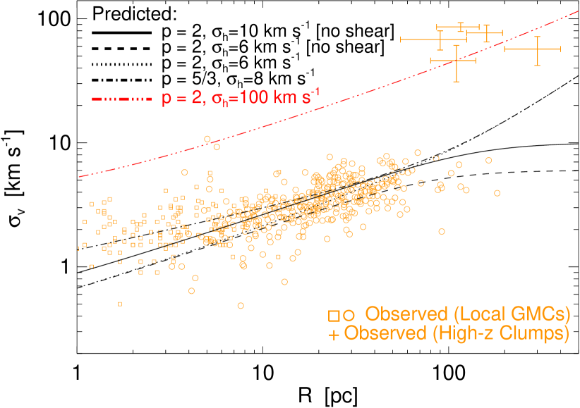
Figure 3: Predicted GMC linewidth-size relation. Different lines correspond to different model assumptions: specifically we vary the turbulent spectral index ($p$), the absolute normalization of the system (amounting to the velocity dispersion $\sigma_{h}^{2}$ at scale $=h$), and whether or not we include disk shear in the “velocity” $\sigma_{v}$. Note that in the models here, $\sigma_{h}$ is not freely varied, it is predicted from the global parameters of the system via our marginal stability assumption. The velocity $\sigma_{v}$ is the one-dimensional linewidth (using $\sigma^{2}=c_{s}^{2}+v_{t}^{2}$) for each cloud at the time of collapse, $R$ is the three-dimensional collapse radius. On scales below $\sim h$, the Monte Carlo results are approximately a power-law with slope $\sigma_{v}\propto R^{0.5}$ (Eq. 35). We compare observations of clouds in the MW and local galaxies, compiled in Bolatto et al. (2008, circles) and Heyer et al. (2009, squares), appropriately corrected to the same quantities. The agreement is good – even for $p=5/3$, for which large-scale effects make the relation slightly steeper than the naive expectation $\sigma_{v}\propto R^{(p-1)/2}$; moreover the marginal stability assumption predicts the normalization accurately. We also compare individual high-redshift molecular “clumps” in extremely gas-rich, rapidly star-forming lensed galaxies in Swinbank et al. (2011, crosses with error bars), which form in much more dense disks (much larger $\Sigma_{\rm disk}$); these lie well above the extrapolation of the relation for MW-like properties. However, if we compare the predictions for a model with the observed $\sigma_{h}\approx 100\,{\rm km\,s^{-1}}$ of their host disks, the agreement is good. Clouds in the MW center, which has intermediate $\Sigma_{\rm disk}$ between these extremes, lie correspondingly between these curves (see Oka et al., 2001).

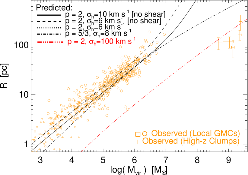
Figure 4: Size-mass relation of clouds, in the same style as Figure 3. The observations from Bolatto et al. (2008) use the virial mass estimator $M_{\rm vir}\equiv 5\,\sigma_{v}^{2}\,R/G$; those from Heyer et al. (2009) and Swinbank et al. (2011) are derived from the CO luminosity. The agreement with observations is good, and the scaling is an approximate power-law with slope $R\propto M^{0.5}$ (approximately constant $\Sigma_{\rm cloud}\sim 100\,M_{\sun}\,{\rm pc^{-2}}$; Eq. 36). Again, the high-redshift clumps lie off the “typical” local galaxy relations; however a model of a more dense disk with $\sigma_{h}\approx 100$ agrees well. Similarly, MW-center clumps lie between the extremes shown (Oka et al., 2001).

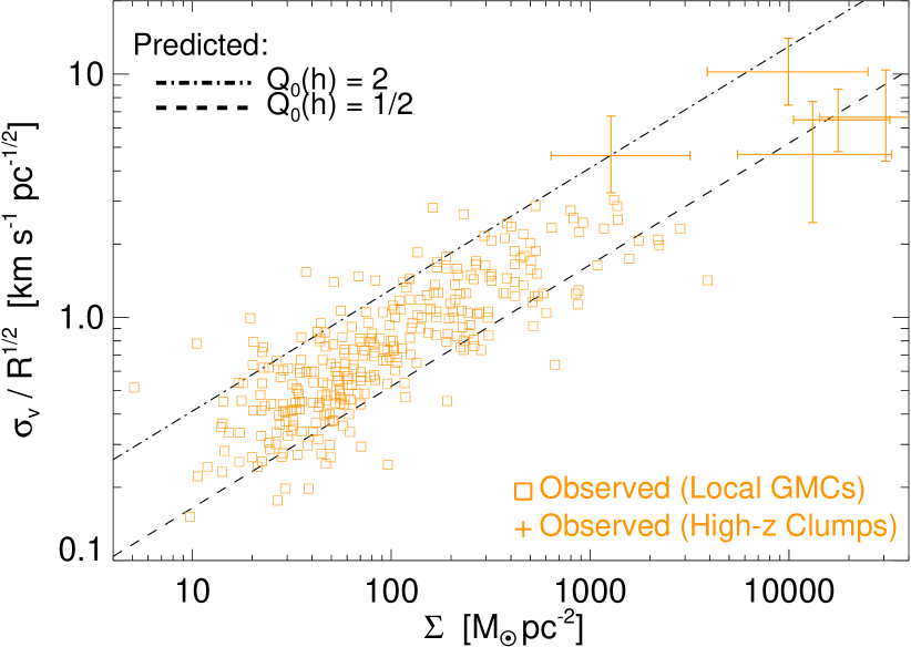
Figure 5: Residuals from the linewidth-size relation for bound clouds as a function of disk/region surface density $\Sigma$, in the style of Figure 3. Because we define clouds as self-gravitating, the different predicted lines (from different turbulent spectra) in Figs. 3-4 collapse to a single line in this plot. So we instead plot the predicted lines for an assumed global stability parameter $Q_{0}\approx 0.5-2.0$. Unbound clouds/overdensities will have higher $\sigma_{v}$, but are not the collapsed objects followed here.

4 Size-Mass & Linewidth-Size Relations

We can also use our model to predict the scaling laws obeyed by GMCs “at collapse.”

The linewidth-size relation follows trivially from our assumed turbulent power spectrum. The exact $\sigma_{v}(R)$ relation is plotted in Figure 3 for power-law turbulent slopes of $p=5/3$ and $p=2$, with the normalization set by requiring a marginally stable disk with MW-like surface density. We can define the line width either as just the turbulent width, or the turbulent width plus the contribution from disk shear $\sigma_{v}^{2}(R)=v_{t}^{2}+\kappa^{2}\,R^{2}$; the distinction is unimportant for typical observed scales, but shear is predicted to contribute significantly to the velocities of the largest GMCs when $R\gtrsim h$. We compare with observations compiled from the MW and other local group galaxies from Bolatto et al. (2008) and Heyer et al. (2009).

In the regime above the sonic length and below the scale height, this is just a simple power law with $\sigma_{v}(R)\propto R^{(p-1)/2}$, i.e. $\approx 0.5$ for $p=2$ or $\approx 0.33$ for $p=5/3$. This is essentially an assumption of our model (although it follows from basic turbulent conditions); more interesting is that the normalization can be predicted from the assumption of marginal stability ($Q\approx 1$), giving

$$\sigma_{v}(R)\approx 0.4\,{\rm km\,s^{-1}}\,{\Bigl{(}}\frac{\langle\Sigma_{\rm disk}\rangle}{10\,M_{\sun}\,{\rm pc}^{-2}}{\Bigr{)}}^{0.5}{\Bigl{(}}\frac{R}{{\rm pc}}{\Bigr{)}}^{0.5}$$ (35)

This agrees well with the observed relation. In the full solution, because of the change in dimensionality above the scale $h$, the relationship flattens if we consider only turbulent velocities; it becomes steeper, however, with the inclusion of the shear term.

This model also specifically predicts a residual dependence in the normalization of the linewidth-size relation that scales as $\langle\Sigma_{\rm disk}\rangle^{1/2}$, where $\langle\Sigma_{\rm disk}\rangle$ is the large-scale mean disk surface density. We stress that this is not necessarily the same as a dependence on the local cloud $\Sigma_{\rm cloud}$ (over a wide dynamic range, in fact, $\Sigma_{\rm disk}$, hence $\Sigma_{\rm cloud}$, is similar). This is also, by definition, for bound objects, not for un-bound overdensities on small scales. The predicted dependence is shown indirectly in Figure 3, and directly in Figure 5, where we compare with the observations compiled in Heyer et al. (2009) in local galaxies and in Swinbank et al. (2011) for massive star-forming molecular complexes in lensed, high-redshift galaxies. These sample extremely different environments, and are indeed offset in the linewidth-size relation. However, the magnitude of their offsets is in good agreement with that predicted here. The galaxies in Swinbank et al. (2011) have an average surface density of $\sim 10^{3}\,M_{\sun}\,{\rm pc^{-2}}$, and a correspondingly very large measured $\sigma_{h}\approx 100\,{\rm km\,s^{-1}}$ (as expected for $Q_{0}(h)\approx 1$); normalizing the predicted linewidth-size relation for these properties, we expect an order of magnitude larger $\sigma_{v}$ at fixed size. Clouds observed in the MW center (Oka et al., 2001), which has a higher mean surface density than the local neighborhood but generally lower than estimated for the high-redshift systems, lie neatly between the predicted curves for the local and high-redshift cases (a mean offset of $\sim 3-5$ relative to the local clouds, corresponding to a factor of $\sim 10-30$ higher $\Sigma_{\rm disk}$, about what is expected for the observed exponential profile). Similar offsets are known in other local galaxies with high surface densities, such as mergers and starburst galaxies (Wilson et al., 2003; Rosolowsky & Blitz, 2005).

As discussed in Hopkins et al. (2012), a dependence of exactly this sort is seen in high-resolution hydrodynamic simulations as well. In the observations, this normalization dependence has sometimes been interpreted as a consequence of magnetic support or confining external pressure (see the discussion in Blitz & Rosolowsky, 2006; Bolatto et al., 2008; Heyer et al., 2009), but in this context magnetic fields and pressure confinement are not explicitly present – such a scaling is a much more broad consequence of the simple Jeans requirements for collapse in any marginally stable environment.

The size-mass relation follows from the critical density $\rho_{c}$ derived in § 2.1, by simply inverting Eqn 14. We plot the exact prediction in Figure 4. In the regime above the sonic length but below the disk scale-height, recall that a power-law turbulent cascade gives the simple condition $\rho_{c}=k^{2}\,v_{t}(k)^{2}/(4\pi G)\propto R^{p-3}$, so $R\propto M^{1/p}$, i.e. $R\propto M^{1/2}$ for $p\approx 2$, very similar to the observed power-law scaling. The normalization also follows – for MW-like global conditions

$$R_{\rm cloud}(R\gg{\ell}_{\rm sonic},\,R\ll h)\approx 1.4\,\sigma_{0.4}^{-1}\,{\rm pc}\,{\Bigl{(}}\frac{M_{\rm cloud}}{300\,M_{\rm sun}}{\Bigr{)}}^{0.5}$$ (36)

where $\sigma_{0.4}$ is the normalization of the turbulent velocities $v_{t}=\sigma_{0.4}\times{0.4\,{\rm km\,s^{-1}}}\,(R/{\rm pc})^{1/2}$. This corresponds to an approximately constant cloud surface density in agreement with Larson’s laws: in projection $\Sigma_{\rm cloud}\approx 100\,M_{\sun}\,{\rm pc^{-2}}$ at the time of collapse. Note that re-calculating this for $p=5/3$ only changes the slope from $0.5$ to $0.6$, well within the observational uncertainty. This will also alter behavior at the highest masses, but this is not significant until well above the mass function break. There does however appear to be tentative evidence for such a transition in the observations shown in Figure 4. As expected from the behavior of the linewidth-size relation, clouds in high density environments – which will have a higher $\sigma_{0.4}$ in Eqn. 36 above – are offset to lower $R$ at fixed $M_{\rm cloud}$; we show the same model prediction for the high-redshift systems in good agreement with the observations. Once again, MW center clouds and other local systems in environments with higher densities are similarly offset.

As discussed in § 3.5, fully extending the models here to the scales of dense cores is beyond the scope of this paper. However, we expect these cores, if self-gravitating, to obey the scaling in Figure 5. This means that if they form inside of high-density GMCs, we can (approximately) think of the “parent” GMC surface density as similar to the background $\langle\Sigma_{\rm disk}\rangle$ term in Eqn. 35, and might expect them to have higher dispersions at fixed sizes. This has been seen in suggested from observations (Ballesteros-Paredes et al., 2011a), as part of a quasi-hierarchical gravitational collapse, similar to the predictions here. Of course, some regions can have much higher $\sigma_{v}$ at fixed $R$ and be simply not self-gravitating; these will not lie on the relation in Figure 5 (they will be offset to higher $\sigma_{v}/R^{1/2}$). This may, in turn, give rise to a dependence of the linewidth-size relation on the tracers and extinction threshold adopted, as observed (Goodman et al., 1998; Lombardi et al., 2010)

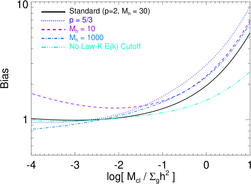
Figure 6: Predicted linear bias $b$ – i.e. the amplitude of spatial clustering – as a function of GMC mass (allowing for clouds inside of bound over densities). We plot this for our standard model and model variations in Figure 2, in dimensionless units. Low-mass GMCs are weakly biased or anti-biased – they simply trace the dense gas. The highest-mass GMCs are strongly clustered – they preferentially trace global overdensities (e.g. spiral arms, galaxy nuclei, etc.).

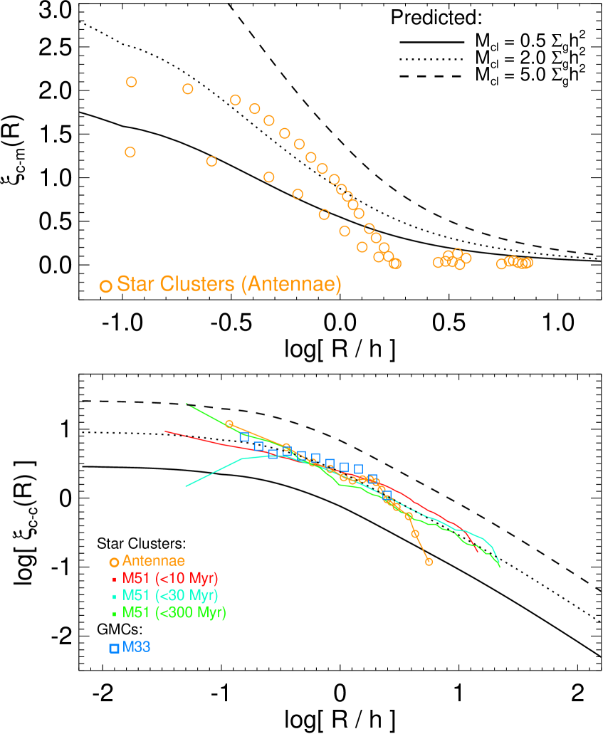
Figure 7: Comparison of the predicted correlation function $\xi(R)$ of bound gas objects/GMCs (lines) with the observed correlation functions of young star clusters. We show the predicted values for three different masses (essentially a normalization difference in the correlation function, corresponding to the bias $b$ in Fig. 6). For lower masses, $b$ changes weakly, and for higher masses the MF is exponentially suppressed, so this covers the interesting range. We plot radii in units of the scale height $h$, in which the correlation function is dimensionless. Top: $\xi_{\rm cm}$, the cross-correlation between bound objects and gas mass (defined in Eq. 42). We compare the observed cross-correlation between young star clusters (which should trace the locations – regardless of how efficiently they form – of their “parent” GMCs) and CO gas maps measured in the Antennae by Zhang et al. (2001). We compare the two youngest $\sim 100$ cluster samples (sampling two different regions and mass ranges), with ages $\lesssim 5\,$Myr and $\sim 3-16$ Myr. We do not know the masses of the progenitor GMCs, but they are likely to be in this range, since these are the most massive young star clusters in the galaxy (the more massive sample has the higher $|\xi_{\rm cm}|$). Despite this being a disturbed system, the agreement is reasonable. Bottom: $\xi_{\rm mm}$, the auto-correlation function of bound objects. We again compare this measured for the young star clusters in the Antennae (orange circles). We also compare the young $\sim 1000$ star cluster autocorrelation function in M51 (which is not disturbed), measured by Scheepmaker et al. (2009) for age intervals $2.5-10$, $10-30$, and $30-300$ Myr (red, cyan, green, respectively). Especially in the youngest samples, the agreement is good. We compare the same, measured directly for GMCs with mass $\sim 2\,\Sigma_{g}\,h^{2}$ in M33 from Engargiola et al. (2003); again the agreement is good.

5 Spatial Clustering of GMCs

In analogy to dark matter halos, we can use the excursion set formalism to also determine the spatial clustering and correlation function strength of these bound sub-units. Following Mo & White (1996), the excess abundance of collapsing objects (relative to the mean abundance) in a sphere of radius $R_{0}$ with mean density $\delta_{0}$ is

$$\delta_{\rm coll}(R_{1},\,\delta_{c,\,1}\,|\,R_{0},\,\delta_{0})\equiv\frac{\mathcal{N}(1|0)}{n(M_{1})\,V_{0}}-1$$ (37)

where $n(M_{1})$ is the average abundance of objects of mass $M_{1}$ (from the mass function) and $\mathcal{N}(1|0)$ is the number of collapsing objects in a region of radius $R_{0}$ (variance $S_{0}$) with fixed overdensity $\delta_{0}$.

5.1 Linear Bias

If $\delta_{c}$ were constant, $\mathcal{N}(1|0)$ can be determined analytically and is simply

$$\mathcal{N}(1|0)=\frac{\rho_{c,\,1}\,V_{0}}{M_{1}}\,\frac{\delta_{c,\,1}-\delta_{0}}{\sqrt{2\pi}\,(S_{1}-S_{0})^{3/2}}\,\exp{{\Bigl{[}}-\frac{(\delta_{c,\,1}-\delta_{0})^{2}}{2\,(S_{1}-S_{0})}{\Bigr{]}}}\,\frac{{\rm d}\,S_{1}}{{\rm d}M_{1}}$$ (38)

(Bond et al., 1991). In the regime where $R_{0}\gg R_{1}$, so $\Delta_{0}\ll\Delta_{1}$, this simplifies to

$$\delta_{\rm coll}\approx{\Bigl{(}}\frac{\nu_{1}^{2}-1}{\delta_{c,\,1}}{\Bigr{)}}\,\delta_{0}=b(M_{1})\,\delta_{0}$$ (39)

where $b(M_{1})$ is defined as the linear bias of objects of mass $M_{1}$.

The barrier $\delta_{c}$ here is not constant. However, for arbitrary $\delta_{c}(M)$, we can calculate $\mathcal{N}(1|0)$ exactly by repeating our Monte Carlo excursion from § 3.1, but instead of beginning with initial conditions $S=0$, $\delta=0$ for each walk, we begin at scale $S=S_{0}$ with density $\delta=\delta_{0}$. The bias $b(M_{1})$ is then just the ratio of $\delta_{\rm coll}/\delta_{0}$ for small $\delta_{0}$.

Figure 6 plots the bias as a function of cloud mass. A couple of key properties are clear. At high masses above the exponential cutoff in the mass function, the bias increases rapidly. This is qualitatively similar to what is seen for dark matter halos: because such systems are exponentially rare, they will tend to be strongly biased towards the few regions with substantial large-scale over densities. Physically, this corresponds to gas overdensities in the disk on scales larger than the scale-height $h$, i.e. a preferential concentration of the most massive GMCs in global instabilities such as spiral arms, bars, and $\sim$kpc-scale massive star-forming complexes, rather than their being randomly distributed across the gas. At intermediate masses below the mass function break, where most of the cloud mass lies, the bias is weak (order unity), so most of the mass in clouds simply traces most of the gas mass in general. We stress that this does not necessarily mean clouds are randomly distributed over the disk as a whole; it means they are unbiased relative to the gas mass distribution. But at low masses, the bias again rises (weakly). This is related to the anti-hierarchical nature of cloud formation: the bias here is driven by clouds which form via fragmentation from other clouds.

We can approximate these exact results using our previous approximate fitting functions for the mass function (Equation 23 & 29) modified (as with the case of a linear barrier) so $S\rightarrow S_{1}-S_{0}$ and $\nu^{2}\rightarrow(\delta_{c}-\delta_{0})^{2}/(S_{1}-S_{0})$. Neglecting the clouds-in-clouds problem (i.e. including those clouds), we obtain the approximate

$$b_{\rm cic}(M_{1})\approx\frac{\nu_{1}^{2}-1+\nu_{1}\,{\rm d}\ln\rho_{1}/{\rm d}\sigma_{1}}{\delta_{c,\,1}\,(1+\nu_{1}^{-1}{\rm d}\ln\rho_{1}/{\rm d}\sigma_{1})}$$ (40)

Which in practice is a small ($\sim 10-20\%$) correction to Equation 39. If we exclude clouds-in-clouds,

$$b(M_{1})\approx\frac{1}{\delta_{c,\,1}}\,{\Bigl{[}}\nu_{1}^{2}-\frac{\delta_{c,\,1}}{\tilde{B}}{\Bigr{]}}$$ (41)

(where $\tilde{B}$ is defined in Equation 23). This is identical to Eqn. 39 at high masses, but it allows for negative bias at low masses, if $B_{\rm min}\equiv\ln{(\rho_{c,\,{\rm min}}/\rho_{0})}<2$ and $\delta_{c}<\sigma^{2}\,(B_{\rm min}^{-1}-1/2)$. Physically, the fact that Equation 40 is always positive means that the number of bound regions of mass $M_{1}$ inside a large-scale overdensity always increases with $\delta_{0}$. However, for some values of $M_{1}$ and $\delta_{0}$, increasing $\delta_{0}$ more rapidly increases the probability that these regions are themselves inside a larger collapsed region. For a more detailed discussion of the leading-order corrections when considering a moving as opposed to constant barrier $\delta_{c}$, we refer to Sheth et al. (2001).

5.2 The Correlation Function: Theory

Recall, the physical over-density is $\rho/\rho_{0}=\exp{(\delta-\sigma(R)^{2}/2)}$. The correlation function $\xi_{\rm cm}$ between collapsed objects of mass $M_{1}$ and background mass, as a function of radius $R_{0}$, is defined by

$$1+\xi_{\rm cm}(R_{0},\,M_{1}) \equiv\frac{\langle\mathcal{N}(1\,|\,R_{0})\,|\,\rho\rangle}{n(M_{1})\,V_{0}\,\rho_{0}}$$ (42)

$$=\langle(1+\delta_{\rm coll})\,|\,\exp{(\delta_{0}-S[R_{0}]/2)}\rangle_{R_{0}}$$ (43)

$$=\int\,\frac{\mathcal{N}(1|0)}{n(M_{1})\,V_{0}}\,e^{(\delta_{0}-S_{0}/2)}\,q(\delta_{0}\,|\,S_{0})\,{\rm d}\delta_{0}$$ (44)

where the integral is over all $\delta_{0}<\delta_{c}(R_{0})$, and $q(\delta_{0}\,|\,S_{0})$ is a weighting factor defined in Bond et al. (1991) as the probability that the overdensity at a random point, smoothed on a scale $R_{0}$, is $\delta_{0}$ and does not exceed $\delta_{c}(R_{0})$ on any larger smoothing scale.

Equation 44 can be evaluated numerically with the Monte Carlo solution for $\mathcal{N}(1|0)$ and $q(\delta_{0}\,|\,S_{0})$. But at large $R_{0}\gg R_{1}$ (provided $S_{0}\rightarrow 0$ as $R\rightarrow\infty$), it simplifies to just

$$1+\xi_{\rm cm}(R_{0},\,M_{1}) \approx 1+b(M_{1})\,\sigma^{2}(R_{0})\ \ \ \ \ (R_{0}\gg R_{1})$$ (45)

$$=1+b(M_{1})\,\xi_{\rm mm}(R_{0})$$ (46)

This can be shown for any first-crossing distribution by first taking $q\rightarrow p(\delta_{0}\,|\,S_{0})$ since the probability of collapse on larger scales is negligible, and then noting $\exp{(\delta_{0}-S_{0}/2)}\,p(\delta_{0}\,|\,S_{0})=1/\sqrt{2\pi\,S_{0}}\,\exp{(-(\delta_{0}-S_{0})^{2}/2\,S_{0})}$, which becomes a delta function centered at $\delta_{0}=S_{0}$ as $S_{0}\rightarrow 0$.

The auto-correlation function of the mass $\xi_{\rm mm}$ is given by $1+\xi_{\rm mm}\equiv\langle\rho^{2}\rangle/\rho_{0}^{2}=\exp{(S_{0})}$, so $\xi_{\rm mm}=\exp{(S_{0})}-1\approx S_{0}=\sigma^{2}(R_{0})$ at large $R_{0}$ is just the variance in the mass field. So the collapsed object-mass correlation function on large scales is then just the bias times the mass autocorrelation function. It is straightforward to verify that the auto-correlation function of collapsed objects is just given by

$$\xi_{\rm cc}\approx b^{2}(M_{1})\,\xi_{\rm mm}\ \ \ \ (R_{0}\gg R_{1})$$ (47)

The correlation functions discussed above are the three-dimensional correlation functions. However, with rare exceptions, it is in general much easier to determine the projected correlation function $\xi_{2d}(R_{p})$, defined so the probability of finding another object in a 2-d annulus $d^{2}{\bf r}$ around a given object is $\langle{\rm d}N/{\rm d}A\rangle\,(1+\xi_{2d})\,d^{2}{\bf r}$. This is straightforward to calculate

$$w_{p}\equiv\xi_{2d}(R_{p})=\frac{\int_{-\infty}^{\infty}\,n_{0}(z)\,\xi_{3d}(\sqrt{R_{p}^{2}+z^{2}})\,{\rm d}z}{\int_{-\infty}^{\infty}n_{0}(z)\,{\rm d}z}$$ (48)

where $z$ is the line-of-sight direction and $n_{0}(z)=n(M)$ is the average abundance. For the typical case of an approximately face-on disk with the exponential vertical profile we have adopted, $n_{0}(z)\propto\exp{(-z/h)}$; however, accounting for this, we should also slightly modify our calculation of $\xi_{3d}$, integrating over $\rho_{0}$ at all central positions with $\mathcal{N}(1\,|\,0\,|\,{\bf x})$ a function of $\rho_{0}({\bf x})$ (since our derivation up to this point implicitly assumed a homogenous background). In either case, at large radii this is just $w_{p}\propto(R/h)\,\xi_{\rm 3d}$.

5.3 Observed GMC & Star Cluster Correlation Functions

In Figure 7, we compare the predicted (two-dimensional) correlation functions to observations. Unfortunately, at present there are no published observations of the GMC-GMC correlation function. However, various groups have measured the correlation functions of young, massive star clusters in nearby systems. Statistically, the positions of such star clusters should trace those of their “parent” GMCs (with greater fidelity as we consider younger star clusters). And although clusters will disperse or be destroyed with time, the correlation function should not be affected so long as this “infant mortality” is not strongly position-dependent (though that is uncertain, if it depends on e.g. tidal fields). This also has the advantage that star clusters can be much longer-lived than GMCs, so allow better statistics. The major uncertainty is that, without knowing the (uncertain) star formation efficiency, the exact mass of the progenitor GMCs is undetermined. However, since the observed systems sample the brightest clusters, we can safely assume that their progenitors were the most massive GMCs (and since the mass function cuts off exponentially, should reflect masses $\sim 1-10$ times the “break” in the mass function).

Scheepmaker et al. (2009) measure the star cluster-star cluster auto-correlation function (which we should compare to the GMC autocorrelation $\xi_{\rm cc}$) in M51 for the brightest $\sim 1000$ star clusters, in three age intervals ($2.5-10$, $10-30$, and $30-300$ Myr). The cluster masses range from $10^{3.5-5}\,M_{\sun}$, which for a few percent star formation efficiency indeed corresponds to the most massive GMCs. The mass scale only affects the bias (normalization) – it is more important to compare the shape of $\xi_{\rm cc}$ – this is invariant in units of $R/h$. With a large number of clusters and a nearly face-on projection, this is the most robust probe over large dynamic range. Zhang et al. (2001) measure in the Antennae the star cluster-star cluster autocorrelation function and the star cluster-gas cross correlation function (tracing the gas in CO maps, which – since the system is quite dense – account for most of the gas mass). Here the geometry is obviously much more complex so the results should be interpreted with additional caution, but the authors do attempt to account for the global structure of the system, and separately measure the correlation functions in different regions. We specifically consider their youngest cluster samples (R and B1), with the brightest $\sim 100$ and $\sim 1000$ objects at ages $\lesssim 5\,$Myr and $\sim 3-16\,$Myr, respectively (masses $\sim 10^{4-6}\,M_{\sun}$). Finally, we attempt to follow the procedure in Scheepmaker et al. (2009) to construct the auto-correlation function for GMCs in M33, using the catalogue in Engargiola et al. (2003), which is both face-on and has a well-defined survey area and completeness limit. Since we cannot properly account for survey edge effects or the global density profile, we simply truncate the correlation function at half the radius inside of which $75\%$ of the identified GMCs are found. Here, we can determine the mean mass in the distribution, which is approximately $\sim 2\,\Sigma_{h}\,h^{2}$ estimated using the parameters from Figure 1 – this is almost exactly the value in the model which gives the best-fit predicted normalization of $\xi(R)$. Given the uncertainties in both observations and the cluster-GMC mapping, the agreement is striking.

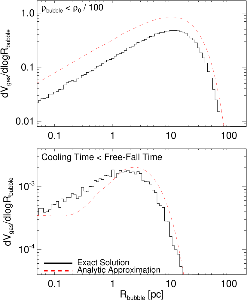
Figure 8: Predicted differential volume fraction in underdense “bubbles” as a function of bubble radius $R$. For illustrative purposes we assume $h=200\,$pc but the scale $R_{\rm bubble}$ scales $\propto h$. Top: Bubbles defined as a proportional under-density $\rho\leq\rho_{0}/100$. Bottom: Bubbles defined as regions where the post-shock cooling time at velocities $\sim v_{t}(R)$ exceeds the free-fall time $\sim 1/\sqrt{G\rho}$. Because determining the cooling time requires absolute units, we normalize the model by assuming $\Sigma=10\,{M_{\sun}\,{\rm pc^{-2}}}$. The exact solution (black solid lines) is compared to the approximate analytic solution (red dashed) from Eq. 49. A broad distribution of underdense regions should be present simply from turbulent velocity divergences, which can have sizes $\sim h$ and contain a large fraction of the disk mass. However, only a small fraction will “self-heat” to temperatures where they cannot cool – “hot” bubbles require energy input from some source (e.g. stellar feedback).

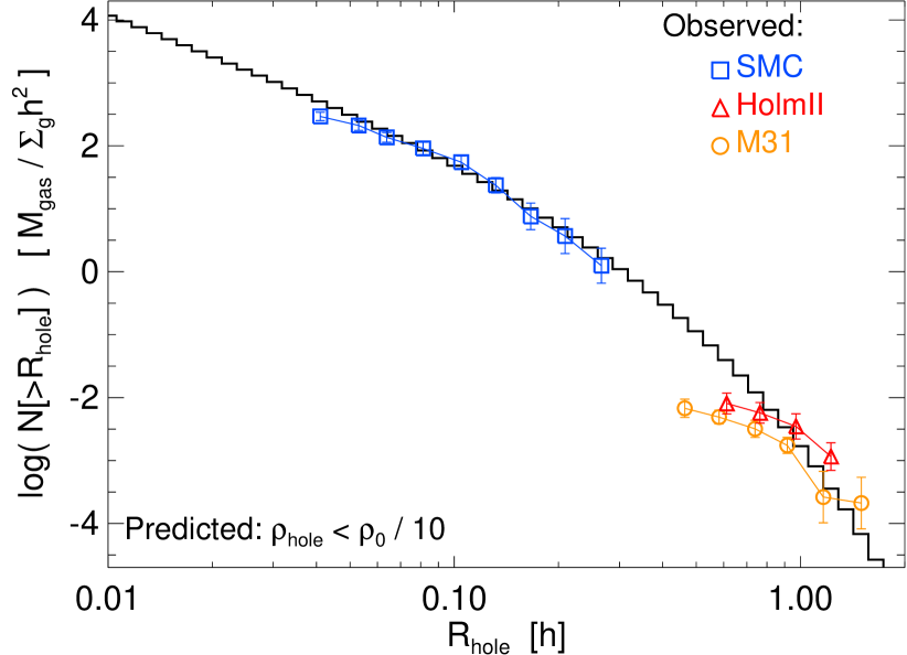
Figure 9: Comparison of predicted and observed hole/bubble radii. We plot the predicted cumulative number of bubbles as a function of bubble size for our standard model, in dimensionless units (bubble size in units of $h$). Here, we assume a simple order-of-magnitude proportional bubble under-density $\rho\leq\rho_{0}/10$. For typical galaxy properties, this also corresponds to densities at which the diffuse galactic UV background will fully ionize the bubble. This allows us to plot all observed systems on the same Figure. We compare the observed HI hole radius functions from radius functions from the SMC (Staveley-Smith et al., 1997), Holmberg II (Puche et al., 1992), and M31 (Brinks & Bajaja, 1986), and normalize them with the observed $M_{\rm gas}$, $\rho_{0}$, $h$ from the same sources. The agreement is good – most, if not all, of the HI “holes” are a natural consequence of turbulent density fluctuations and require no input energy source to “clear them out.”

6 The Distribution of Underdense Bubbles

Just as we used the excursion set formalism to predict the mass function of clouds by identifying objects above a critical over-density $\delta_{c}$, we can also use it to predict the abundance of under-dense regions (“bubbles”) by identifying regions below a critical under-density $\delta_{b}$. We will follow Sheth & van de Weygaert (2004), who apply this formalism to the dark matter halo context to study the distribution of voids.

Generally, the procedure is the same, but considering the mass/radii below $\delta_{b}$ instead of above $\delta_{c}$. However, some additional complications arise. First, unlike the case of collapsing objects where the counting of “clouds in clouds” was potentially valid, here we should clearly count “voids in voids” as simply part of the larger, parent void/bubble. So we again need to specify to the first crossing distribution (the distribution of the largest radii on which trajectories cross $\delta_{b}$). Second, we must also ensure that the void/bubble region is not itself contained inside of a collapsing region (i.e. that $\delta<\delta_{c}$ on all scales above the $\delta_{b}$ crossing), since that would “overwhelm” or “squeeze” the bubble. Third, and most critical for our purposes, a “void” or “bubble” is not obviously well-defined in this context. Because there is no linear expansion here, we cannot derive the equivalent of the shell crossing criterion used for dark matter halo voids, and there is no obvious threshold which is physically as robust as the self-gravity criterion for collapse. We will return to this question and consider different plausible, but ultimately somewhat arbitrary choices of under-density criterion.

If the “bubble” barrier $\delta_{b}$ and the collapse barrier (which must be avoided on scales above the bubble) $\delta_{c}$ were constant, then Sheth & van de Weygaert (2004) show that the first crossing distribution can be analytically re-derived subject to these boundary conditions, to give the fraction of trajectories in bubbles per logarithmic interval ${\rm d}\ln{\nu_{b}}$

$$\nu_{b}\,f_{b}(\nu_{b}) =\sum_{n=1}^{\infty}\,\frac{2n\pi\mathcal{D}^{2}}{\nu_{b}^{2}}\,\sin{(n\pi\mathcal{D})}\,\exp{{\Bigl{(}}-\frac{n^{2}\pi^{2}\mathcal{D}^{2}}{2\nu_{b}^{2}}{\Bigr{)}}}$$ (49)

$$\mathcal{D} \equiv\frac{|\delta_{b}|}{\delta_{c}+|\delta_{b}|}\ ,\ \ \ \ \nu_{b}\equiv\frac{|\delta_{b}|}{S(R)^{1/2}}$$ (50)

Recalling that we are sampling the Eulerian space, we can then trivially translate this to the number density of bubbles per unit radius or mass, e.g.

$$\frac{{\rm d}n}{{\rm d}\ln{R}}=\frac{1}{V_{b}}\,\frac{{\rm d}f}{{\rm d}\ln{R}}=\nu_{b}\,f_{b}(\nu_{b})\,\frac{1}{V_{b}}\,\frac{{\rm d}\ln{\nu_{b}}}{{\rm d}\ln{R}}$$ (51)

where $V_{b}$ is the effective volume of the bubble.

Again, we stress that the barrier is not constant, so we do not know that this will be an accurate approximation. More rigorously, it is straightforward to derive the same first-crossing distribution using the Monte Carlo approach in § 3.1. We follow the identical procedure, but simply record the first crossing of $\delta_{b}(R)$ for those trajectories that cross $\delta(R)<\delta_{b}(R)$ and have not crossed $\delta_{c}(R)$ at any larger scale.

The results of this exact calculation, and the analytic approximation from Equation 49, are shown in Figure 2, for two different choices of $\delta_{b}$. First, we consider a simple under-density criterion: here $\rho_{b}\leq\rho_{0}/100$. There is a very broad distribution of bubbles which satisfy this criterion: it includes several tens of percent of the total mass. The characteristic spatial “bubble scale” is at a factor of $\sim 0.1\,h$, which (for the definitions used here) corresponds very closely to the scale at which the local contributions to density fluctuations ($\Delta S$) are maximized. A large population of such fluctuations must arise for a density distribution similar to Equation 6: because the distribution is lognormal, the median density is $\ln{(\rho_{\rm med}/\rho_{0})}=-\sigma^{2}/2$; i.e. for $\sigma\sim 1.3\,$dex fluctuations, $\rho_{\rm med}\approx 0.01\,\rho_{0}$ so of order half the volume should be in underdense regions. For any fixed (fractional) density threshold $\rho_{b}/\rho_{0}$, the behavior is qualitatively similar, but shifts systematically to smaller scales $R$ and smaller normalization (the total mass in such regions scaling as $\sim\exp{(-\nu_{b}^{2}/2}$) as $\rho_{b}/\rho_{0}$ decreases.

There is nothing physically “special” about such regions – they are simply the low-$\rho$ portion of the density PDF. A more meaningful threshold might be to define “bubbles” as regions where the cooling time becomes longer than the free-fall time. The isothermal temperature $c_{s}$ is however quite low, so this will not be satisfied unless the temperature suddenly increases; for this, consider the shocks occurring in the turbulent medium at $v_{s}\sim v_{t}(R)$. Knowing $E(k)$, we can estimate the distribution of post-shock temperatures and densities for a random Lagrangian parcel, and compare the resulting cooling time to the free-fall time $t_{\rm ff}\approx 0.54/{\sqrt{G\,\rho}}$. Since we are interested in the regime where the cooling time will be long, we can simplify the problem by assuming a strong adiabatic shock and that thermal Brehmsstrahlung dominates the cooling. In this regime, $t_{\rm cool}\equiv n\,k_{B}\,T/\Lambda\,n^{2}\leq t_{\rm ff}$ at densities

$$n_{b}(R)\lesssim 10^{-4}\,{\rm cm^{-3}}\,{\Bigl{(}}\frac{v_{t}(R)}{10\,{\rm km\,s^{-1}}}{\Bigr{)}}^{2}$$ (52)

If we normalize our model to MW-like conditions by assuming $\sigma_{g}(h)\approx 10\,{\rm km\,s^{-1}}$ and $n_{0}=\rho_{0}/\mu m_{p}\approx 1\,{\rm cm^{-3}}$, then this defines $\delta_{b}$. The resulting distribution of bubbles is shown in Figure 8. Qualitatively, the shape of the distribution is similar – it truncates more rapidly at low $R$ because the decrease of turbulent velocities $\langle v_{t}(R)\rangle$ with decreasing $R$ means that the barrier becomes more difficult to cross. The normalization is also significantly lower, corresponding to the lower absolute densities ($\rho_{b}/\rho_{0}\sim 10^{-4}$) needed near scales $\sim h$ to reach this “hot gas” threshold.

In both cases, the analytic approximation of Equation 49 works well for the largest voids (albeit with a factor $\sim 1-1.5$ normalization offset), but is systematically offset for low-mass voids. This is directly a consequence of the moving barriers $\delta_{c}$ and $\delta_{b}$.

In Figure 9, we compare the predicted size function of bubbles (in dimensionless units) to observations of HI “holes.” We compile the observed HI hole size distributions in the SMC (Staveley-Smith et al., 1997), Holmberg II (Puche et al., 1992), and M31 (Brinks & Bajaja, 1986), and scale the normalization of each according to the observed global galaxy properties measured at the radii enclosing half the “holes.” Observations of the LMC (Kim et al., 1999), IC2574 (Walter & Brinks, 1999), and M33 (Deul & den Hartog, 1990) give similar results.

There is no well-defined criterion for selection of “holes” and the density contrasts involved are typically modest, so we simply compare with the prediction for a constant density contrast $\rho_{b}\leq\rho_{0}/10$. This is approximately consistent with the direct estimates of the interior bubble densities/density contrast, and also (for the global properties of these systems) corresponds to densities where even the largest (few hundred pc) holes would become fully ionized either from the diffuse galactic background or a single O/B star inside the “hole.” The agreement is good – if anything, the model predicts more small “holes,” but this may be a question of observational selection/completeness (or a deficit of sources to ionize them). The characteristic hole size is predicted to scale with $h$ (the characteristic radius), giving larger holes in thicker galaxies – a well-observed phenomenon (see Oey & Clarke, 1997; Walter & Brinks, 1999, and references therein).

7 Construction of GMC “Merger Trees” from This Formalism

7.1 General Considerations

One of the most powerful applications of the excursion set approach in galaxy formation is the construction of the extended Press-Schecter “merger trees,” conditional mass functions, and formation histories for dark matter halo populations, which form the foundation of semi-analytic models. This provides a means to statistically link populations in time and self-consistently model their evolution, with whatever additional physics are desired. We now show that the same “merger tree” approach can be applied here, to derive the time evolution of the systems we have thus far considered static.

Before we describe the mechanics of constructing these trees, there are a couple of important physical distinctions that will necessitate a somewhat different treatment from the typical methodology in the dark matter halo EPS formalism.

First, unlike with dark matter halos, there is no reason to believe that bound clouds are “conserved” (modulo their mergers into more massive clouds). In fact we expect from observations that they only live a short time, then are disrupted (Zuckerman & Evans, 1974; Williams & McKee, 1997; Evans, 1999; Evans et al., 2009). So it makes no sense to begin from a present population of clouds and work backwards in time to construct the tree (as is typically done for halo merger trees). Instead, we need to forward-model the time evolution, to allow whatever model physics the user desires to determine whether or not such clouds survive.

Second, we cannot assume that all the mass is in collapsing objects. We must therefore track un-collapsed elements as well, allowing for their possible collapse at later times.

Third, density fluctuations in a turbulent medium clearly do not evolve according to simple linear growth, in the manner of cosmological density perturbations. How, then, can we link a fluctuation at any one time to that at another time? To do this, we will assume that the turbulence is globally steady-state: i.e. that – excepting the behavior of collapsing regions – the turbulent velocity cascade is (statistically) maintained and, as a result, so is the global density PDF. We stress that we are not attempting to model how the turbulence is maintained. In this regime, the density PDF for independent modes on different scales obeys a generalized Fokker-Planck equation, with a diffusion term giving the effectively “random walk” behavior of each Lagrangian density parcel (from small-scale encounters/shocks/accelerations) and a drift term corresponding to damping/relaxation (from viscosity, pressure forces, mixing, and the energetic cost associated with large velocity deviations). Under these conditions, if we know the stationary behavior of the PDF for some variable $x$ is a Gaussian distribution with standard deviation $\sigma_{x}$ and zero mean, then the probability distribution to find the system with value $x$ at time $t$ given an initial distribution with (delta-function) value $x_{0}$ at time $t_{0}=t-\Delta\,t$ is

$$p(x,\,t)\,{\rm d}x =\frac{1}{\sqrt{2\pi\,\tilde{\sigma}_{x}^{2}}}\,\exp{{\Bigl{(}}-\frac{(x-\tilde{x}_{0})^{2}}{2\,\tilde{\sigma}_{x}^{2}}{\Bigr{)}}}$$ (53)

$$\tilde{\sigma}_{x} \equiv\sigma_{x}\,\sqrt{1-\exp{(-2\,[t-t_{0}]/\tau)}}\approx\sigma_{x}\,\sqrt{2\,\Delta t/\tau}$$ (54)

$$\tilde{x}_{0} \equiv x_{0}\,\exp{(-[t-t_{0}/\tau])}\approx x_{0}\,(1-\Delta t/\tau)$$ (55)

where the latter equalities are the series expansion for $\Delta\,t/\tau\ll 1$.

The timescale $\tau$ here is the timescale on which the variance of $x(t)$ with respect to $x_{0}$ grows, normalized by the steady-state variance $\sigma_{x}$, i.e. the timescale of “mixing” in the distribution. More formally the amplitude of the correlation between values in time declines with exponential timescale $\tau$. In supersonic turbulence, this is simply the crossing time

$$\tau=\eta\,t_{\rm cross}=\eta\,R/\langle v_{t}^{2}(R)\rangle^{1/2}$$ (56)

Where $\eta\approx 1$ is a constant which can be calibrated from numerical simulations (Pan & Scannapieco 2010 find $\eta\approx 0.90-1.05$ over the range $\mathcal{M}\sim 1.2-10$).

7.2 The Mechanism of Tree Construction

With these points resolved, it is straightforward to generalize our approach to construct a time-dependent “fragmentation tree.” We outline the methodology below.

(0) Define the variance $S\equiv\sigma^{2}(R)$ and collapse threshold $\delta_{c}(R)$ either directly or from the turbulent power spectrum $E(k)$.

(1) Begin by constructing the initial conditions. Consider a Monte Carlo ensemble of “trajectories,” as in § 3.1. Each trajectory $\delta(R)$ is defined by the values $\Delta\delta_{j}$ on each scale $R_{j}\rightarrow R_{j}-\Delta R$. We are free to choose whatever values of $\Delta\delta_{j}$ define an appropriate initial condition. For example, we can assume that the medium has a density PDF corresponding to “fully developed” turbulence and generate the $\Delta\delta_{j}$ exactly in § 3.1. Or we can begin with a perfectly smooth medium, setting all $\Delta\delta_{j}=0$, and treat all structures self-consistently as they develop. Critically, save the full trajectories $\Delta\delta_{j}$ (full $\delta(R)$) for each member of the Monte Carlo population, including those for which the region is “uncollapsed” ($\delta(R)$ never crosses $\delta_{c}(R)$).

(2) Evolve the system forward by one time step $\Delta t$. For a Fourier-space tophat window, we can evolve the system by perturbing each $\Delta\delta_{j}$ independently according to Equation 53 (obtaining a new, perturbed trajectory $\delta(R,\,t+\Delta t)$). The probability distribution for the perturbed $\Delta\delta_{j}(R,\,t+\Delta t)$ is given by Equation 53 with the appropriate substitutions:

$$\frac{{\rm d}p(\Delta\delta_{j}[t+\Delta t])}{{\rm d}(\Delta\delta_{j}[t+\Delta t])} =$$ (57)

$$\frac{1}{\sqrt{2\pi\psi\,\Delta S}}\, \exp{{\Bigl{(}}-\frac{(\Delta\delta_{j}[t+\Delta t]-\Delta\delta_{j}[t]\sqrt{1-\psi})^{2}}{2\psi\,\Delta S}{\Bigr{)}}}$$

$$\psi \equiv 1-\exp{(-2\,\Delta t/\tau)}$$ (58)

$$\tau \equiv{R}/{\langle v_{t}(R)^{2}\rangle^{1/2}}$$ (59)

This is equivalent to taking

$$\Delta\delta_{j}(t+\Delta t) =\Delta\delta_{j}(t)\,\exp{(-\Delta t/\tau)}$$ (60)

$$+\mathcal{R}\,\sqrt{\Delta S\,(1-\exp{(-2\,\Delta t/\tau)})}$$ (61)

$$\approx\Delta\delta_{j}(t)\,(1-\Delta t/\tau)+\mathcal{R}\,\sqrt{2\,\Delta S\,\Delta t/\tau}$$ (62)

where $\mathcal{R}$ is a Gaussian random number with unity variance. This is done for all $\Delta\delta_{j}$ in the trajectory, giving a new trajectory

$$\delta(R,\,t+\Delta t)\equiv\sum_{j}^{R_{j}>R}\,\Delta\delta_{j}(R_{j},\,t+\Delta t)$$ (63)

which can now be evaluated.

(3) After each timestep, evaluate all trajectories $\delta(R)$ in the Monte Carlo ensemble. If the trajectory did not cross $\delta_{c}(R)$ at any $R$ in the previous time steps – i.e. it represented an uncollapsed region – then either it will remain uncollapsed ($\delta(R)<\delta_{c}(R)$ at all $R$) in the new time step, or it will now cross the barrier at some $R_{\rm c}$. The largest such $R_{\rm c}$ corresponds to the collapse scale, defining a new self-gravitating object with mass $M\equiv 4\pi/3\,\rho_{c}(R_{\rm c})\,R_{\rm c}^{3}$. Physically, this event corresponds to the random density fluctuations from e.g. shocks and other processes pushing this previously “diffuse” gas parcel to densities at which it becomes self-gravitating, and collapses. The trajectory should still be saved, but the mass is now in a self-gravitating object, and the first-crossing scale on which it became self-gravitating should be recorded.

If the trajectory already crossed the barrier at some $R_{\rm c}$, then there are two possibilities. If the trajectory no longer crosses the barrier (or crosses at some smaller radius $R<R_{\rm c}$), it has no effect (continue to save the trajectory, but do not modify the properties of the object). This corresponds to a decline in the “background” density field – however, because the object is self-gravitating, this cannot simply “random walk” the collapsed region back into being uncollapsed. By definition, gravity will prevent such expansion modulo some stronger forces applied in the model (discussed below). However, if the trajectory now crosses the barrier $\delta_{c}(R)$ at some larger $R_{\rm c,\,new}>R_{\rm c}$, this corresponds to a mass growth event for the collapsed object. The mass of the cloud should be updated to $M_{\rm c,\,new}\rightarrow(4\pi/3)\,\rho_{c}(R_{\rm c,\,new})\,R_{\rm c,\,new}^{3}>M_{\rm c}$, and the first-crossing/collapse radius updated to $R_{\rm c}\rightarrow R_{\rm c,\,new}$. Unlike the case with dark matter halos (where all mass is locked into halos, so every growth event is a halo-halo merger), the fact that there is un-collapsed mass means that some of these events correspond to cloud-cloud mergers, while others correspond to previously “diffuse” gas reaching a self-gravitating threshold. If this distinction is needed, the method in Somerville & Kolatt (1999) can easily be generalized to decompose the mass growth $\Delta\,M=M_{\rm c,\,new}-M_{\rm c}$ into a “progenitor cloud” and “diffuse” mass function.

(4) Apply whatever cloud-specific physics are desired, in the timestep $\Delta t$, for the population of identified bound objects. This is where the essence of any semi-analytic model enters. One could assume clouds continue to collapse under gravity, that they form stars (either instantaneously, or with some efficiency in time, or with some association with clump-clump mergers), that they form molecules (based on e.g. their local column densities and SFRs), that they disrupt on some timescale or as some function of star formation/feedback properties, that they accrete “diffuse” material (e.g. Bondi-Hoyle accretion, which as a non-local effect is not included in the “growth events” in step (3)). There are obviously a huge range of model physics than can be included.

One particularly interesting application of this model to bound clouds is to consider recursively applying the same analysis within each cloud, to determine the bound sub-units into which it will fragment. For a given bound cloud, if the model defines some average density and turbulent power spectrum (for example, assuming they maintain their properties at collapse, virialize and contract by dissipation, etc), then the procedure to determine the mass function and other properties of these “sub-clumps” is exactly identical to the procedure for the “parent” clumps, but with the revised or re-normalized density/mass/velocity properties of the “parent” clump.

(5) Repeat steps (2)-(4), to continue to evolve the system in time as desired.

We also note that despite our stated assumption of steady-state turbulence, it is perfectly possible to make the global parameters of the model (e.g. densities, masses, assumed structural properties, turbulent power spectrum) arbitrary functions of time and/or consequences of the explicit “cloud physics” put into the model. For example, allowing for continuous accretion and/or gas exhaustion to systematically change the normalization of the density with time, or allowing turbulent velocities to damp in the absence of some feedback from clouds to “pump” them. Likewise, it is possible to repeat or rescale these experiments in different “intervals” corresponding to the average properties at different radii in a galaxy disk (corresponding to e.g. an exponential profile) so that together, the Monte-Carlo ensemble can represent the properties of the entire galaxy disk. The only implicit assumption in the above is that these properties evolve slowly, relative to the local mixing/equilibration time for the turbulence (a crossing time).

Figure 10: Fraction of the total ISM gas mass and volume in bound clouds, as a function of the cloud lifetime (in units of the cloud crossing time). We follow a full population of clouds through a time-dependent “merger/fragmentation tree” constructed as described in § 7.2. When a bound region collapses, we allow it to remain collapsed for a time $t_{\rm lifetime}=L\,t_{\rm dyn}=L/(R_{\rm c}/v_{t}[R_{\rm c}])$ ($t_{\rm dyn}$ is the crossing time at the moment of becoming bound); when this time expires the mass is returned to the “diffuse” (non-bound) ISM. A lifetime $\sim 1-5\,t_{\rm dyn}$ gives a fraction in bound units consistent with the observed ISM; larger values lock all mass into bound units (and will over-predict the GMC MF), smaller values the opposite.

Figure 11: Mass fraction which collapses into bound sub-units per free-fall time (defined as $t_{\rm ff}=0.54/\sqrt{G\,\rho_{0}}\approx h/\sigma(h)=\Omega^{-1}$, if $Q=1$), for systems which are marginally stable on large scales, as a function of Mach number (normalized at large scales, $\mathcal{M}_{h}=\mathcal{M}(h)$). Solid line is the analytic prediction from running a suite of models as in Figure 10, in which clouds remain bound (are removed from the “diffuse” medium). Given the same global stability, systems with higher $\mathcal{M}$ have larger dispersions and more rapidly cross the collapse barrier, but the scaling is weak. Without some additional physics to disrupt bound objects, mass collapses at $\sim M_{\rm gas}/t_{\rm dyn}$ independent of the maintenance of the large-scale cascade. We compare with the results of high-resolution simulations of turbulence. First, idealized forced turbulent box simulations with collapse into sink particles from Vázquez-Semadeni et al. (2003) (hydro) and Padoan & Nordlund (2011) (hydro and MHD). For each, we select the runs which most closely match the “marginally stable” assumption ($\alpha_{\rm vir}\approx 1$ for the box). Second, full disk galaxy simulations with no stellar feedback from Hopkins et al. (2011) with “collapse rates” defined as the modeled star formation rate (which occurs in bound gas at densities $n>1000\,{\rm cm^{-3}}$, on $\sim 1\,$pc scales). As shown therein, these all maintain $Q\approx 1$ via gravitational instabilities; $\mathcal{M}_{h}$ is taken as the mass-weighted average $\mathcal{M}$ for the disk gas averaged over a spatial scale $=h$. Error bars show the scatter in both quantities. The excursion-set model successfully predicts the results of fully nonlinear hydrodynamic simulations, within the scatter between different simulations/realizations.

7.3 Example: The Rate of Collapse into Bound Units and Constraints on Cloud Lifetimes

It is not our intention here to present a full semi-analytic model for clouds. However, we briefly illustrate how such a model might be used with a highly simplified implementation.

We follow steps (0)-(5) above, with the standard (dimensionless) parameters and $p=2$ power spectrum adopted throughout this paper. The specification of the power spectrum and assumption of marginal stability completely specify the model, except for the physics applied to bound objects, step (4).

For these bound objects, we apply a toy “zero physics” model, with the only goal being to see the effects of different “cloud lifetimes” on the distribution of the ISM. When an object has collapsed, we allow it to remain collapsed for a “lifetime” $L\,t_{\rm cross}$ where $t_{\rm cross}$ is the crossing time of the cloud at the time of collapse $R_{\rm c}/v_{t}(R_{\rm c})\approx 1/\sqrt{G\rho_{c}}$. When this time has elapsed, we “destroy” the cloud and recycle its material, in practice by “resetting” the associated path (setting all $\Delta\delta_{j}=0$ for the designated path). The trajectory then re-grows with time according to Equation 53, essentially randomizing the density in a crossing time.

For any choice of $L$, the mass function and mass fraction in bound objects will eventually converge to a steady state value (in practice, this requires only a couple of disk crossing times). Figure 10 shows the resulting steady-state mass fraction in collapsed and bound objects, as a function of $L$ from $L\ll 1$ to $L\gg 1$. When $L\ll 1$, the mass fraction in collapsed objects is negligible, and declines $\propto L$ at lower $L$ (as expected for systems with a constant formation rate). When $L\gg 1$, the mass in collapsed objects quickly saturates near unity (with an exponentially suppressed residual non-collapsed mass). In this regime, because clouds live much longer then the typical cloud-cloud merger time, the mass function also shifts to higher and higher masses (roughly shifting the break/maximum GMC mass $M_{\rm break}\propto L$).

Only choices with $L\sim 1-5$ yield reasonable total collapsed masses in steady state (of order tens of percent, but with order tens of percent of the mass also in the inter-clump medium), and agreement with the observed GMC mass function. This is easy to understand: because the density distribution evolves on a crossing time, the rate of addition of mass to the GMC population is $\sim\exp{(-\nu(h_{\rm max})^{2}/2)}\,M_{\rm gas}/t_{\rm dyn}(h_{\rm max})$ where $h_{\rm max}\sim h$ represents the most unstable wavelength, where $\nu(h_{\rm max})$ is order unity. So the lifetime for an appropriate steady-state should be $L\sim\exp{(\nu_{\rm max}^{2}/2)}\sim$ a few.

This relates directly to idealized hydrodynamic simulations of turbulent boxes with self-gravity. These experiments have found that even when a forcing term is included to maintain the turbulent cascade at all times (for a box which is globally stable against collapse), a large fraction (tens of percent) of the mass in the box will reach densities where it becomes self-gravitating (presumably turning into stars, if there is no feedback) in a free-fall time (see e.g. the discussion in Padoan & Nordlund, 2011). Here, we have calculated the exact same quantity analytically (on a galaxy-wide scale).

We can estimate the rate of collapse, in the absence of feedback, by simply assuming clouds are arbitrarily long-lived and then calculating the time for some fraction of the mass to be bound into clouds. If we perform this exercise as a function of the dimensionless Mach number $\mathcal{M}_{h}$ (for a $p=2$ spectrum), we obtain

$$\frac{t_{\rm consumption}}{t_{\rm dyn}(h)}\approx 1.5-0.34\sqrt{\ln{(1+3\mathcal{M}_{h}/8)}}$$ (64)

Where we define $t_{\rm consumption}$ as the time to $1/2$ of gas consumed and $t_{\rm dyn}(h)\equiv h/\langle v_{t}^{2}(h)\rangle^{1/2}\approx\Omega^{-1}$. Note the weak and positive dependence of the collapse rate on $\mathcal{M}_{h}$ – this comes from our assumption of marginal stability for the disk as a whole – at a fixed stability level, larger $\mathcal{M}$ means a broader density PDF, and so increases the collapse rate. We compare the resulting collapse rate as a function of $\mathcal{M}$ to full numerical hydrodynamic simulations: both simulations of small-scale, idealized turbulent boxes (in which self-gravitating regions at the resolution limit are identified as sink particles), and large-scale simulations of galaxy disks (without stellar feedback) in which self-gravitating regions become “star particles.” In all cases we compare models with marginal stability on the largest scales. Our analytic calculation is in good agreement with the full numerical calculation.

8 Discussion

We have used the fact that the ISM is super-sonically turbulent on a wide range of scales to develop a rigorous excursion-set model for the formation, structure, and time evolution of gas structures (e.g. GMCs, massive clumps/cores, and voids) in the ISM. We derive the conditions for self-gravitating collapse in a turbulent medium applicable on both small scales (the Jeans condition) and large scales (the Toomre criterion); together with the assumption that the density distribution in super-sonic turbulence is approximately lognormal, we use this to derive the statistical properties of the smoothed density field on all scales as a function of smoothing scale $R$. We show, then, that (with some appropriate modifications from the standard cosmological case) this becomes a well-defined barrier crossing problem (albeit one with a complicated barrier structure), for which the full methodology of excursion set theory can be applied.

We use this model to calculate the mass function of bound gas structures (over the entire dynamic range from near the sonic length to masses well above the Jeans mass). We do so in a rigorous manner that explicitly resolves the “cloud in cloud” problem. We show that this agrees extremely well with observed GMC mass functions in the MW and other nearby galaxies. This prediction is nearly independent of any free parameters, with the only input being the mass and size of the galaxies. Even galaxies such as M33, which has been extensively discussed as apparently exhibiting a deviant GMC mass function slope, are accurately predicted. The generic properties of the mass function are rigorously derived: an exponential cutoff above the Jeans mass (because large-scale density fluctuations are suppressed by disk shear) and a faint-end power-law slope close to, but slightly shallower than, $-2$ (which deviates logarithmically with mass). It is near $-2$ (equal mass on all scales) generically because the collapse threshold (being relative to $\ln{\rho}$) is only a logarithmic function of scale and gravity is scale free; but slightly shallower because collapse is more difficult on small scales for any realistic turbulent power spectrum. We show this is robust to large variations in mach number and velocity power spectrum shape, and even to large deviations from exact log-normality in the density PDF.

The same model also predicts the linewidth-size and size-mass relations of these clouds, in good agreement with observations. The linewidth-size relation slope is a generic result of the assumed turbulent power spectrum, but its normalization is predicted by the assumption that the disk must be globally stable; the size-mass relation follows from the collapse criteria. Second-order corrections (from e.g. disk shear) make both less sensitive to the turbulent index in the range $p\sim 5/3-2$. Residuals from these relations naturally emerge as a function of the galaxy surface density, in good agreement with recent comparisons of GMC properties in the MW outskirts and center and in high-redshift galaxies.

The excursion set theory also allows us to rigorously predict the spatial correlation function and clustering properties of these clouds; we predict that most of the mass in clouds should be weakly biased (i.e. trace the overall gas density), but the most massive clouds will preferentially be biased towards large-scale overdensities (e.g. spiral arms). We construct the auto-correlation function of GMCs from the catalogue of clouds in M33 and show this agrees extremely well with that predicted for clouds of the same mass. If we assume that young star clusters should more or less trace the positions of their “parent” clouds, then we can also compare their clustering. We show that both the star cluster-gas mass cross-correlation function, and the star cluster auto-correlation function observed in the youngest clusters in the Antennae and M51 agrees well with that predicted, over the observed range of scales $R<0.1\,h$ to $R>10\,h$.

Using similar logic as applied to the GMC mass function, we can predict the size and mass distributions of under-dense “bubbles” in the ISM. We show that a large fraction of the ISM should be in highly under-dense “bubbles” with $\rho\lesssim 0.01-0.1\,\rho_{0}$, and that the characteristic size should scale with scale height $h$, as a natural consequence of turbulent fluctuations. These require no additional “power source” other than whatever maintains the turbulence. If we consider the distribution of bubble/hole sizes below a density threshold such that they should be easily ionized by the galactic background, we show that this agrees very well with the HI “hole” size distribution observed in nearby galaxies such as the SMC, M31, and Holmberg II. The energetic cost of “creating” these bubbles is negligible, as compared to the nominally large $PdV$ work required if they were excavated by e.g. SNe explosions, and they do not require any internal stars/star clusters to power their expansion. Even if some are powered in this manner, it is clear that many are not. This resolves a long-standing problem, as follow-up observations of these “holes” have consistently failed to observe SNe remnants or other evidence of young stellar populations “powering” the hole expansion (see e.g. Rhode et al., 1999; Weisz et al., 2009). We stress that turbulence alone will not explain the gas in bubbles being hot: the fraction of holes predicted to have a cooling time much longer than a dynamical time from turbulent shocks alone is small. But it will explain their sizes, expansion, and densities. Where they are heated, it requires a much smaller amount of energy, at that point, to simply “leak into” the bubble.

We generalize the excursion-set model of the ISM to allow the construction of time-dependent “merger/fragmentation trees” which can be used to follow the evolution of clouds and construct semi-analytic models for GMC and star-forming populations. We provide explicit recipes to construct these trees. We use a simple example to show that, if clouds were not destroyed by some feedback process in a timescale $\sim 1-5$ crossing times, then all the ISM mass would be “consumed” (collapsing to arbitrarily high densities in bound objects) even if the large scale turbulent cascade were maintained. Absent such feedback, we show that our analytic calculation can predict with reasonable accuracy the collapse rates seen in full nonlinear hydrodynamic (and MHD) simulations of both turbulent boxes and galaxies over a wide range of characteristic Mach numbers.

It is striking that we can predict so many properties of a highly complex, chaotic, and – unlike the cosmological case – fully nonlinear system with a single model. This suggests that a wealth of properties of the ISM and GMC populations are generic consequences of collapse in a supersonically turbulent medium with a characteristic “scale” set by gravitational instability in a gaseous disk. This explains why different simulations (Ostriker et al., 2001; Dobbs, 2008; Bournaud et al., 2007; Tasker & Tan, 2009; Tasker, 2011) have been able to reproduce various aspects of these observations, despite including very different physics for cooling/feedback/star formation/magnetic fields, and in some cases clearly failing to reproduce other (probably feedback-dependent) properties such as the observed star formation rates and galactic winds (see e.g. the discussion in Hopkins et al., 2012, and references therein). What is remarkable is that our theory allows us to calculate these nonlinear properties analytically, over a large dynamic range, and in quantitative agreement with the observations.

We should also stress that this model does not necessarily imply or require that the ISM structure be rigorously self-similar or fractal: that may be true, but it is a much stronger statement about the structure of $S(R)$ and $B(R)$ (compared to our assumptions). In our default model those happen to be approximately scale free over some range, but there are at least two scales – the sonic length and disk scale height – above/below which behavior changes. The application of this model also does not necessarily imply the ISM is “hierarchical” either in the cosmological sense or the sense of Vazquez-Semadeni (1994) (see § 1). In fact in the cosmological sense of the term, the predicted structure is more appropriately “anti-hierarchical,” in that collapse tends to proceed “top-down.” Large scales $\sim h$ are most unstable and contain most of the turbulent power, and we have shown that most self-gravitating objects on small scales are formed by “fragmenting out” of larger structures (i.e. form within parent GMCs; these are the low-mass GMCs predicted if we ignore the cloud-in-cloud problem, which are much more abundant than isolated counterparts). In contrast, in the cosmological case, small structures form first, and “subhalos” are only a small fraction of the population at most masses.

There are many interesting potential future directions for these models. Many of our assumptions can be made more general, and the model made more accurate. For example, if the gas is not isothermal, or when magnetic fields and global gravitational forces are strong, some deviations from lognormality are expected. We have argued that should not qualitatively change our conclusions, but it is possible to rigorously treat this regime, by extending the excursion set formalism to non-Gaussian fields (as developed in e.g. Matarrese et al., 2000; Afshordi & Tolley, 2008; Maggiore & Riotto, 2010b). The Monte Carlo excursion set approach is also completely generalizeable to treat correlated random walks, so that arbitrary higher-order structure functions (i.e. correlations between fluctuations on different scales) can be incorporated – it is only a convenient simplifying assumption to assume strict locality (see the review in Zentner, 2007). Near and below the sonic length (or in the warm/diffuse ISM), when the turbulence is sub/transsonic, additional corrections to the power spectrum could be included. Magnetic fields can also be included as more than just a correction to the effective sound speed, if their power spectrum is well determined (see e.g. Kim et al., 2002). We have also assumed that the density and velocity field are not directly coupled, but it is in principle straightforward to allow for a direct correlation between the local density and velocity fluctuations, to follow both with a higher-dimensional random walk, and to incorporate this in the collapse criterion (see e.g. Sheth & Tormen, 2002). We have neglected large-scale gradients in e.g. the disk surface density profile; this should not be important for most GMCs since their sizes are $\lesssim h$, but a more rigorous calculation of global properties (e.g. the large-scale spatial distribution of clouds) could consider each radial annulus in turn with some global mass profile. Our derivation of the collapse barrier also assumes spherical collapse, when in fact most GMCs are ellipsoidal or triaxial. In the cosmological context, ellipsoidal collapse is a well-studied problem (Sheth et al., 2001), and can be incorporated via an appropriate change of the barrier shape (although the appropriate parameters are usually determined by reference to numerical simulations); however, if the cosmological case is any guide, the differences should be small (tens of percent level).

The lack of dependence of many of the predicted observables on the detailed properties of turbulence is, in one sense, reassuring (and explains agreement between previous models with different physics). On the other hand, unfortunately, it means that observations have a limited ability to discriminate between these different physical scenarios. Of course, the ISM is not all highly supersonic, and there will be some regimes in which the model here is not appropriate. Implicitly, our model assumes that the ISM can cool efficiently (cooling time short relative to the dynamical time), so that the turbulence remains super-sonic. This is easily satisfied inside the radii that include most star formation in galactic disks. However, at sufficiently large radii and very low gas densities, the galactic and cosmological ionizing backgrounds maintain gas disks as fully ionized with $Q>1$. Even in the star-forming disk, there are bubbles of hot gas that may escape before cooling. And a significant fraction of the mass in the “warm” ISM medium is turbulent and bound, but has comparable thermal sound speeds and turbulent velocities (i.e. is transsonic rather than super-sonic). In this regime, it is necessary to account explicitly for the effects of heating and cooling, for example as in the model of Ostriker et al. (2010), since only regions pushed to a critical density where cooling becomes efficient will behave as we assume. Even in this regime, however, the internal structure of those cooling regions/GMCs should be treatable with the model here, but it should be emphasized that this model is most applicable to the cold/rapidly cooling gas rather than the extended low-density gas.

There is also a huge space of physical predictions which can be explored with this model that we have not yet addressed, some of which may be more sensitive tests of the properties of turbulence and ISM structure formation. Using the time-dependent formulation, the growth of of GMCs via turbulent density fluctuations, mergers, and accretion can be rigorously analytically calculated. By allowing for global evolution of self-gravitating regions, it is possible to self-consistently follow features that nominally appear to contradict the model – for example, following a simple model whereby, once “detached” from the background, a cloud collapses spherically will naturally predict a power-law tail to high densities (in collapsing regions), even though we can continue to use the same treatment for each cloud internally. Together with a semi-analytic model for star formation in such units, their destruction via feedback can also be followed analytically in a self-consistent statistical model for the population. Global feedback effects can also be predicted – for example, many authors have used the cosmological formulation of the problem to study the reionization history of the Universe and evolving size distribution of HII regions (e.g. Haiman et al., 2000; Furlanetto et al., 2004). It is straightforward to adapt their approach to the problem here to predict the properties of galactic HII regions, SNe blastwaves, and ionizing photon escape fractions. The model can be extended iteratively (downwards in scale) within GMCs, to calculate the properties of dense collapsing subregions (cores). Extended sufficiently in scale, the model can even be used to predict the stellar IMF in each subregion, following Hennebelle & Chabrier (2008) – with a model determined on galactic scales. These scales, being closer to the sonic length, should exhibit much stronger dependence on the actual turbulent structure than the galactic-scale quantities we calculate here (as seen in other analytic calculations and simulations; see Ballesteros-Paredes et al., 2006; Hennebelle & Chabrier, 2009), and might be used to break degeneracies between different models for the ISM microphysics.

References

- Afshordi & Tolley (2008) Afshordi, N., & Tolley, A. J. 2008, PhRvD, 78, 123507
- Anathpindika (2011) Anathpindika, S. 2011, New Astronomy, 16, 323
- Ballesteros-Paredes et al. (2006) Ballesteros-Paredes, J., Gazol, A., Kim, J., Klessen, R. S., Jappsen, A.-K., & Tejero, E. 2006, ApJ, 637, 384
- Ballesteros-Paredes et al. (2011a) Ballesteros-Paredes, J., Hartmann, L. W., Vázquez-Semadeni, E., Heitsch, F., & Zamora-Avilés, M. A. 2011a, MNRAS, 411, 65
- Ballesteros-Paredes et al. (2011b) Ballesteros-Paredes, J., Vazquez-Semadeni, E., Gazol, A., Hartmann, L. W., Heitsch, F., & Colin, P. 2011b, MNRAS, 416, 1436
- Begelman & Shlosman (2009) Begelman, M. C., & Shlosman, I. 2009, ApJL, 702, L5
- Blitz & Rosolowsky (2006) Blitz, L., & Rosolowsky, E. 2006, ApJ, 650, 933
- Block et al. (2010) Block, D. L., Puerari, I., Elmegreen, B. G., & Bournaud, F. 2010, ApJL, 718, L1
- Bolatto et al. (2008) Bolatto, A. D., Leroy, A. K., Rosolowsky, E., Walter, F., & Blitz, L. 2008, ApJ, 686, 948
- Boldyrev et al. (2002) Boldyrev, S., Nordlund, Å., & Padoan, P. 2002, ApJ, 573, 678
- Bonazzola et al. (1987) Bonazzola, S., Heyvaerts, J., Falgarone, E., Perault, M., & Puget, J. L. 1987, A&A, 172, 293
- Bond et al. (1991) Bond, J. R., Cole, S., Efstathiou, G., & Kaiser, N. 1991, ApJ, 379, 440
- Bournaud et al. (2007) Bournaud, F., Elmegreen, B. G., & Elmegreen, D. M. 2007, The Astrophysical Journal, 670, 237
- Bournaud et al. (2010) Bournaud, F., Elmegreen, B. G., Teyssier, R., Block, D. L., & Puerari, I. 2010, MNRAS, 409, 1088
- Bower (1991) Bower, R. G. 1991, MNRAS, 248, 332
- Bowman (1996) Bowman, J. C. 1996, Journal of Fluid Mechanics, 306, 167
- Brinks & Bajaja (1986) Brinks, E., & Bajaja, E. 1986, A&A, 169, 14
- Burgers (1973) Burgers, J. 1973, The nonlinear diffusion equation: asymptotic solutions and statistical problems (D. Reidel Pub. Co.)
- Bussmann et al. (2008) Bussmann, R. S., et al. 2008, ApJL, 681, L73
- Chandrasekhar (1951) Chandrasekhar, S. 1951, Royal Society of London Proceedings Series A, 210, 26
- Cole et al. (2000) Cole, S., Lacey, C. G., Baugh, C. M., & Frenk, C. S. 2000, MNRAS, 319, 168
- Deul & den Hartog (1990) Deul, E. R., & den Hartog, R. H. 1990, A&A, 229, 362
- Dobbs (2008) Dobbs, C. L. 2008, MNRAS, 391, 844
- Elmegreen (1987) Elmegreen, B. G. 1987, ApJ, 312, 626
- Elmegreen (2002) —. 2002, ApJ, 564, 773
- Engargiola et al. (2003) Engargiola, G., Plambeck, R. L., Rosolowsky, E., & Blitz, L. 2003, ApJS, 149, 343
- Evans et al. (2009) Evans, N. J., et al. 2009, ApJS, 181, 321
- Evans (1999) Evans, II, N. J. 1999, ARA&A, 37, 311
- Federrath et al. (2010) Federrath, C., Roman-Duval, J., Klessen, R. S., Schmidt, W., & Mac Low, M.-M. 2010, A&A, 512, A81+
- Fukui et al. (2008) Fukui, Y., Kawamura, A., Minamidani, T., Mizuno, Y., Kanai, Y., Mizuno, N., Onishi, T., Yonekura, Y., Mizuno, A., Ogawa, H., & Rubio, M. 2008, ApJS, 178, 56
- Furlanetto et al. (2004) Furlanetto, S. R., Zaldarriaga, M., & Hernquist, L. 2004, ApJ, 613, 1
- Gao & Solomon (2004) Gao, Y., & Solomon, P. M. 2004, ApJ, 606, 271
- Goldsmith et al. (2008) Goldsmith, P. F., Heyer, M., Narayanan, G., Snell, R., Li, D., & Brunt, C. 2008, ApJ, 680, 428
- Goodman et al. (1998) Goodman, A. A., Barranco, J. A., Wilner, D. J., & Heyer, M. H. 1998, ApJ, 504, 223
- Goodman et al. (2009a) Goodman, A. A., Pineda, J. E., & Schnee, S. L. 2009a, ApJ, 692, 91
- Goodman et al. (2009b) Goodman, A. A., Rosolowsky, E. W., Borkin, M. A., Foster, J. B., Halle, M., Kauffmann, J., & Pineda, J. E. 2009b, Nature, 457, 63
- Haiman et al. (2000) Haiman, Z., Abel, T., & Rees, M. J. 2000, ApJ, 534, 11
- Hennebelle & Chabrier (2008) Hennebelle, P., & Chabrier, G. 2008, ApJ, 684, 395
- Hennebelle & Chabrier (2009) —. 2009, ApJ, 702, 1428
- Heyer et al. (2009) Heyer, M., Krawczyk, C., Duval, J., & Jackson, J. M. 2009, ApJ, 699, 1092
- Hopkins (2012) Hopkins, P. F. 2012, MNRAS, in press, arXiv:1201.4387
- Hopkins et al. (2011) Hopkins, P. F., Quataert, E., & Murray, N. 2011, MNRAS, 417, 950
- Hopkins et al. (2012) —. 2012, MNRAS, 421, 3488
- Kim & Ryu (2005) Kim, J., & Ryu, D. 2005, ApJL, 630, L45
- Kim et al. (1999) Kim, S., Dopita, M. A., Staveley-Smith, L., & Bessell, M. S. 1999, AJ, 118, 2797
- Kim et al. (2002) Kim, W.-T., Ostriker, E. C., & Stone, J. M. 2002, ApJ, 581, 1080
- Klessen (2000) Klessen, R. S. 2000, ApJ, 535, 869
- Kowal et al. (2007) Kowal, G., Lazarian, A., & Beresnyak, A. 2007, ApJ, 658, 423
- Kritsuk et al. (2007) Kritsuk, A. G., Norman, M. L., Padoan, P., & Wagner, R. 2007, ApJ, 665, 416
- Krumholz & McKee (2005) Krumholz, M. R., & McKee, C. F. 2005, ApJ, 630, 250
- Lacey & Cole (1993) Lacey, C., & Cole, S. 1993, MNRAS, 262, 627
- Larson (1981) Larson, R. B. 1981, MNRAS, 194, 809
- Lemaster & Stone (2009) Lemaster, M. N., & Stone, J. M. 2009, in Revista Mexicana de Astronomia y Astrofisica, vol. 27, Vol. 36, Revista Mexicana de Astronomia y Astrofisica Conference Series, 243–+
- Li et al. (2004) Li, P. S., Norman, M. L., Mac Low, M.-M., & Heitsch, F. 2004, ApJ, 605, 800
- Li & Nakamura (2006) Li, Z.-Y., & Nakamura, F. 2006, ApJL, 640, L187
- Lombardi et al. (2010) Lombardi, M., Alves, J., & Lada, C. J. 2010, A&A, 519, L7
- Mac Low & Klessen (2004) Mac Low, M.-M., & Klessen, R. S. 2004, Reviews of Modern Physics, 76, 125
- Maggiore & Riotto (2010a) Maggiore, M., & Riotto, A. 2010a, ApJ, 711, 907
- Maggiore & Riotto (2010b) —. 2010b, ApJ, 717, 526
- Matarrese et al. (2000) Matarrese, S., Verde, L., & Jimenez, R. 2000, ApJ, 541, 10
- McKee & Ostriker (2007) McKee, C. F., & Ostriker, E. C. 2007, ARA&A, 45, 565
- Mo & White (1996) Mo, H. J., & White, S. D. M. 1996, MNRAS, 282, 347
- Nordlund & Padoan (1999) Nordlund, Å. K., & Padoan, P. 1999, in Interstellar Turbulence; Cambridge University Press, ed. J. Franco & A. Carraminana (Cambridge, UK: Cambridge University Press), 218–+
- Oey & Clarke (1997) Oey, M. S., & Clarke, C. J. 1997, MNRAS, 289, 570
- Oka et al. (2001) Oka, T., Hasegawa, T., Sato, F., Tsuboi, M., Miyazaki, A., & Sugimoto, M. 2001, ApJ, 562, 348
- Ostriker et al. (1999) Ostriker, E. C., Gammie, C. F., & Stone, J. M. 1999, ApJ, 513, 259
- Ostriker et al. (2010) Ostriker, E. C., McKee, C. F., & Leroy, A. K. 2010, ApJ, 721, 975
- Ostriker et al. (2001) Ostriker, E. C., Stone, J. M., & Gammie, C. F. 2001, ApJ, 546, 980
- Padoan et al. (2004) Padoan, P., Jimenez, R., Nordlund, Å., & Boldyrev, S. 2004, Physical Review Letters, 92, 191102
- Padoan et al. (2006) Padoan, P., Juvela, M., Kritsuk, A., & Norman, M. L. 2006, ApJL, 653, L125
- Padoan & Nordlund (2002) Padoan, P., & Nordlund, Å. 2002, ApJ, 576, 870
- Padoan & Nordlund (2011) —. 2011, ApJ, 730, 40
- Padoan et al. (1997) Padoan, P., Nordlund, A., & Jones, B. J. T. 1997, MNRAS, 288, 145
- Pan & Scannapieco (2010) Pan, L., & Scannapieco, E. 2010, ApJ, 721, 1765
- Passot & Vazquez-Semadeni (1998) Passot, T., & Vazquez-Semadeni, E. 1998, PhRvE, 58, 4501
- Pineda et al. (2009) Pineda, J. E., Rosolowsky, E. W., & Goodman, A. A. 2009, ApJL, 699, L134
- Press & Schechter (1974) Press, W. H., & Schechter, P. 1974, ApJ, 187, 425
- Price et al. (2011) Price, D. J., Federrath, C., & Brunt, C. M. 2011, ApJL, 727, L21
- Puche et al. (1992) Puche, D., Westpfahl, D., Brinks, E., & Roy, J.-R. 1992, AJ, 103, 1841
- Rhode et al. (1999) Rhode, K. L., Salzer, J. J., Westpfahl, D. J., & Radice, L. A. 1999, AJ, 118, 323
- Romeo (1992) Romeo, A. B. 1992, MNRAS, 256, 307
- Rosolowsky (2005) Rosolowsky, E. 2005, PASP, 117, 1403
- Rosolowsky & Blitz (2005) Rosolowsky, E., & Blitz, L. 2005, ApJ, 623, 826
- Rosolowsky et al. (2008) Rosolowsky, E. W., Pineda, J. E., Kauffmann, J., & Goodman, A. A. 2008, ApJ, 679, 1338
- Scalo et al. (1998) Scalo, J., Vazquez-Semadeni, E., Chappell, D., & Passot, T. 1998, ApJ, 504, 835
- Scheepmaker et al. (2009) Scheepmaker, R. A., Lamers, H. J. G. L. M., Anders, P., & Larsen, S. S. 2009, A&A, 494, 81
- Schmidt et al. (2009) Schmidt, W., Federrath, C., Hupp, M., Kern, S., & Niemeyer, J. C. 2009, A&A, 494, 127
- Schmidt et al. (2008) Schmidt, W., Federrath, C., & Klessen, R. 2008, Physical Review Letters, 101, 194505
- Scoville et al. (1987) Scoville, N. Z., Yun, M. S., Sanders, D. B., Clemens, D. P., & Waller, W. H. 1987, ApJS, 63, 821
- Sheth et al. (2001) Sheth, R. K., Mo, H. J., & Tormen, G. 2001, MNRAS, 323, 1
- Sheth & Tormen (2002) Sheth, R. K., & Tormen, G. 2002, MNRAS, 329, 61
- Sheth & van de Weygaert (2004) Sheth, R. K., & van de Weygaert, R. 2004, MNRAS, 350, 517
- Slyz et al. (2005) Slyz, A. D., Devriendt, J. E. G., Bryan, G., & Silk, J. 2005, MNRAS, 356, 737
- Somerville & Kolatt (1999) Somerville, R. S., & Kolatt, T. S. 1999, MNRAS, 305, 1
- Stanimirovic et al. (1999) Stanimirovic, S., Staveley-Smith, L., Dickey, J. M., Sault, R. J., & Snowden, S. L. 1999, MNRAS, 302, 417
- Staveley-Smith et al. (1997) Staveley-Smith, L., Sault, R. J., Hatzidimitriou, D., Kesteven, M. J., & McConnell, D. 1997, MNRAS, 289, 225
- Swinbank et al. (2011) Swinbank, A. M., Papadopoulos, P. P., Cox, P., Krips, M., Ivison, R. J., Smail, I., Thomson, A. P., Neri, R., Richard, J., & Ebeling, H. 2011, ApJ, 742, 11
- Tasker (2011) Tasker, E. J. 2011, ApJ, 730, 11
- Tasker & Tan (2009) Tasker, E. J., & Tan, J. C. 2009, ApJ, 700, 358
- Toomre (1977) Toomre, A. 1977, ARA&A, 15, 437
- Vandervoort (1970) Vandervoort, P. O. 1970, ApJ, 161, 87
- Vazquez-Semadeni (1994) Vazquez-Semadeni, E. 1994, ApJ, 423, 681
- Vázquez-Semadeni et al. (2003) Vázquez-Semadeni, E., Ballesteros-Paredes, J., & Klessen, R. S. 2003, ApJL, 585, L131
- Vázquez-Semadeni & García (2001) Vázquez-Semadeni, E., & García, N. 2001, ApJ, 557, 727
- Vazquez-Semadeni & Gazol (1995) Vazquez-Semadeni, E., & Gazol, A. 1995, A&A, 303, 204
- Walter & Brinks (1999) Walter, F., & Brinks, E. 1999, AJ, 118, 273
- Weisz et al. (2009) Weisz, D. R., Skillman, E. D., Cannon, J. M., Dolphin, A. E., Kennicutt, Jr., R. C., Lee, J., & Walter, F. 2009, ApJ, 704, 1538
- Williams & McKee (1997) Williams, J. P., & McKee, C. F. 1997, ApJ, 476, 166
- Wilson et al. (2003) Wilson, C. D., Scoville, N., Madden, S. C., & Charmandaris, V. 2003, ApJ, 599, 1049
- Wong et al. (2009) Wong, T., Hughes, A., Fukui, Y., Kawamura, A., Mizuno, N., Ott, J., Muller, E., Pineda, J. L., Welty, D. E., Kim, S., Mizuno, Y., Murai, M., & Onishi, T. 2009, ApJ, 696, 370
- Wong et al. (2008) Wong, T., et al. 2008, MNRAS, 386, 1069
- Zentner (2007) Zentner, A. R. 2007, International Journal of Modern Physics D, 16, 763
- Zhang et al. (2001) Zhang, Q., Fall, S. M., & Whitmore, B. C. 2001, ApJ, 561, 727
- Zuckerman & Evans (1974) Zuckerman, B., & Evans, II, N. J. 1974, ApJL, 192, L149