Nested Canalyzing Depth and Network Stability

Abstract

We introduce the nested canalyzing depth of a function, which measures the extent to which it retains a nested canalyzing structure. We characterize the structure of functions with a given depth and compute the expected activities and sensitivities of the variables. This analysis quantifies how canalyzation leads to higher stability in Boolean networks. It generalizes the notion of nested canalyzing functions (NCFs), which are precisely the functions with maximum depth. NCFs have been proposed as gene regulatory network models, but their structure is frequently too restrictive and they are extremely sparse. We find that functions become decreasingly sensitive to input perturbations as the canalyzing depth increases, but exhibit rapidly diminishing returns in stability. Additionally, we show that as depth increases, the dynamics of networks using these functions quickly approach the critical regime, suggesting that real networks exhibit some degree of canalyzing depth, and that NCFs are not significantly better than functions of sufficient depth for many applications of the modeling and reverse engineering of biological networks.

1 Introduction

A large influx of biological data on the cellular level has necessitated the development of innovative techniques for modeling the underlying networks that regulate cell activities. Several discrete approaches have been proposed, such as Boolean networks [8], logical models [17], and Petri nets [5]. In particular, Boolean networks have emerged as popular models for gene regulatory networks [1, 12]. However, not all Boolean functions accurately reflect the behavior of biological systems, and it is imperative to recognize classes of functions with biologically relevant properties. One such notable class is the canalyzing functions, introduced by Kauffman [8], whose behavior mirrors biological properties described by Waddington [20]. The dynamics of Boolean networks constructed using these functions are of considerable interest when determining their modeling potential. Random Boolean networks constructed using such functions have been shown to be more stable than networks using general Boolean functions, in the sense that they are insensitive to small perturbations [10]. Karlssona and Hörnquist [7] explore the relationship between the proportion of canalyzing functions and network dynamics. In [10], the authors further expand the canalyzation concept and introduce the class of nested canalyzing functions (NCFs). In [11], networks of NCFs are shown to exhibit stable dynamics. Also, Nikolajewa, et al. [13] divide NCFs into equivalence classes based on their representation and show how the network dynamics are influenced by choice of equivalence class. Nested canalyzing functions have a very restrictive structure and become increasingly sparse as the number of input variables increases [6]. Also, it is possible that not all variables exhibit canalzying behavior. Hence, a relaxation of the nested canalyzing structure is necessary.

In this article, we further explore canalyzation by analyzing functions that retain a partially nested canalyzing structure. We quantify the degree to which a function exhibits this canalyzing structure by a quantity we call the nested canalyzing depth. Functions of depth $d$ generalize the nested canalyzing functions, because NCFs are the special case of when $d=k$, where $k$ is the number of Boolean variables. In Section 3, we demonstrate notable properties of these partially nested canalyzing functions, and show that their representation is unique. This leads to a theorem about the structure of functions of depth $d$, which generalizes a result in [6] about NCFs. In Section 4, we compute the expected activities and sensitivities of functions given their canalyzing depths, which are extensions of results of Shmulevich and Kauffman [18] about activities and sensitivities of canalyzing functions. We prove that as canalyzing depth increases, functions become less sensitive to perturbations in the input; however, the marginal benefit incurred by adding further canalyzing variables sharply decreases. As a result, functions of larger depth provide an improvement in sensitivity over general canalyzing functions, but imposing a fully nested canalyzing structure provides little benefit over functions of sufficient canalyzing depth. Finally, in Section 5, we use Derrida plots to show that dynamics of networks constructed using more structured functions rapidly approach the well-known critical regime, whereas networks with functions of relatively few nested canalyzing variables remain in the chaotic phase. This is in contrast to the findings of Kauffman et al. [11], but in agreement with recent work of Peixoto [16], and it further supports the biological utility of certain canalyzing functions.

2 Nested Canalyzing Depth

A Boolean function $f(x)=f(x_{1},\dots,x_{k})$ is canalyzing if it has a variable $x_{i}$ for which some input $x_{i}=a_{i}$ implies $f(x)=b_{i}$ for some $b_{i}\in\{0,1\}$. In this case, $x_{i}$ is a canalyzing variable, the input $a_{i}$ is its canalyzing value, and the output value $b_{i}$ when $x_{i}=a_{i}$ is the corresponding canalyzed value. Note that if $f$ is constant, then every variable is trivially canalyzing.

If a canalyzing variable $x_{i}$ does not receive its canalyzing input $a_{i}$, then the output is some function $g_{i}(\hat{x}_{i})$, where $\hat{x}_{i}=(x_{1},\ldots,x_{i-1},x_{i+1},\ldots,x_{k})$. If $g_{i}$ is constant, $x_{i}$ is called a terminal canalyzing variable of $f$. Note that for each $i\neq j$, $x_{j}$ is then trivially canalyzing in $g_{i}$.

If $g_{i}$ is not constant, we ask whether it too is canalyzing. If so, there is a canalyzing variable $x_{j}$ with canalyzing input $a_{j}$, and when $x_{j}\neq a_{j}$, the output of $f$ is a function $g_{ij}(\hat{x}_{ij})$, which may or may not be canalyzing. Here, $\hat{x}_{ij}$ denotes $x$ with both $x_{i}$ and $x_{j}$ omitted. Eventually, this process will terminate when the function $g$ is either constant or no longer canalyzing.

Definition 1.

Let $f(x_{1},\ldots,x_{k})$ be a Boolean function. Suppose that for a permutation $\sigma\in S_{k}$, an integer $d>0$ and a Boolean function $g(x_{\sigma(d+1)},\ldots,x_{\sigma(k)})$,

$$f=\left\{\begin{array}[]{lll}b_{1}&&x_{\sigma(1)}=a_{1}\\ b_{2}&&x_{\sigma(1)}\neq a_{1},\;x_{\sigma(2)}=a_{2}\\ b_{3}&&x_{\sigma(1)}\neq a_{1},\;x_{\sigma(2)}\neq a_{2},\;x_{\sigma(3)}=a_{3}\\ \;\vdots&&\;\vdots\\ b_{d}&&x_{\sigma(1)}\neq a_{1},\ldots,\;x_{\sigma(d-1)}\neq a_{d-1},\;x_{\sigma(d)}=a_{d}\\ g&&x_{\sigma(1)}\neq a_{1},\ldots,\;x_{\sigma(d)}\neq a_{d}\end{array}\right.$$ (1)

where either $x_{\sigma(d)}$ is a terminal canalyzing variable (and hence $g$ is constant), or $g$ is non-constant and none of the variables $x_{\sigma(d+1)},\ldots,x_{\sigma(k)}$ are canalyzing in $g$. Then $f$ is said to be a partially nested canalyzing function. The integer $d$ is called the active nested canalyzing depth of $f$, and the full nested canalyzing depth of $f$ is $d$ if $g$ is non-constant, and $k$ otherwise. The sequence $x_{\sigma(1)},\dots,x_{\sigma(k)}$ is called a canalyzing sequence for $f$.

If we speak of simply the “canalyzing depth” or “depth” of a function, we are referring to the full nested canalyzing depth. In the next section, we will show that the depth is well-defined, i.e., that it does not depend on the choice of $\sigma\in S_{k}$. The class of nested canalyzing functions (NCFs) [6, 10] are precisely those with active depth $k$. A constant function (all $2^{k}$ entries in the truth table are the same) is not an NCF by the classical definition, but changing a single value in the truth table suddenly makes it nested canalyzing. In our set-up, both of these functions have full depth $k$. Constant functions have active depth 0. For completeness, we will say that a non-canalyzing function has active and full nested canalyzing depth 0.

Canalyzing and nested canalyzing functions have been used in gene network models because they possess biologically relevant features [20]. For example, in a gene regulatory network, a collection of $k$ genes that affect the expression level of a particular gene can be modeled with a $k$-variable Boolean function. While it is believed that some of these relationships are canalyzing (e.g., if $A$ is expressed, then $B$ is not expressed, regardless of the states of the other genes), it is unreasonable to expect that all relevant genes will act in a nested canalyzing manner. For instance, transcription factors in gene regulatory networks likely display canalyzing behavior, while other proteins do not. Thus, situations will arise in which nested canalyzing functions do not fully capture the dynamics of biological systems. For example, in the gene regulatory network of the cell cycle in Saccharomyces cerevisiae, genes Cdc14 and Cdc20 are the only canalyzing inputs for the Swi5 gene. The remaining function is constant, which does not fit Kauffman’s definition of nested canalyzing, nor can this gene’s behavior be modeled with an NCF [12]. Thus, when reverse engineering a biological network with partial data, the rigid NCF structure is restrictive and likely inappropriate to model the behavior of the system. Also, the number of NCFs becomes rapidly sparse in the set of Boolean functions as $k$ increases. For instance, the proportion of NCFs in 6 variables is on the order of $10^{-15}$ [6]. Because of this sparsity, it is unlikely that a nested canalyzing function fits a given data set. We will show why functions with less than full canalyzing depth exhibit nearly identical key features as NCFs with regards to activities, sensitivities, and stability, promoting their potential use in biological models.

Example 1.

Consider the function defined as

$$f(x_{1},x_{2},x_{3},x_{4})=x_{2}\wedge(\neg x_{1}(\wedge(x_{3}\textup{ XOR }x_{4})))\,,$$

which is similar to Example 2.4 in [6]. There is a canalyzing sequence $x_{2},x_{1}$, with $a_{2}=b_{2}=0$, and $a_{1}=1$ and $b_{1}=0$. The remaining function $g(x_{3},x_{4})=x_{3}\textup{ XOR }x_{4}$ is not canalyzing in either variable. Therefore, $f$ is a PNCF of active and full depth $2$.

3 Properties of Partially Nested Canalyzing Functions

Proposition 1.

Let $f(x)$ be a $k$-variable Boolean function. Then

• If $x_{i}=a_{i}$ implies $f(x)=b_{i}$, and $x_{i}\neq a_{i}$ leaves $g_{i}(\hat{x}_{i})$, then at least half of the truth table values of $f$ must be $b_{i}$.

• If exactly half the truth table values of $f$ are $b_{i}$, then either $x_{i}$ is terminally canalyzing, or $f$ is a non-canalyzing function.

Proof.

The statement in (i) follows because $x_{i}=a_{i}$ for exactly half of the input values in the truth table. The corresponding output value must be $b_{i}$ for at least these inputs. To show (ii), suppose that $f$ is canalyzing, and $x_{i}=a_{i}$ implies $f(x)=b_{i}$. By (i), $x_{i}\neq a_{i}$ implies $f(x)=\neg b_{i}$. Therefore, $g(\hat{x}_{i})$ is constant and $x_{i}$ is terminally canalyzing. ∎

The canalyzing depth of a function can be computed in a divide-and-conquer manner described in Algorithm 1. The algorithm scans the truth table for a canalyzing variable, and upon finding one, removes the columns for which the canalyzing variable takes the canalyzing input value. This is repeated until no more canalyzing variables are present or a constant function remains. Proposition 1 and the structure of the truth table imply that if there is a tie for $b$, then there is a terminally canalzying variable or there are no canalyzing variables. Therefore, it is not necessary to test both $b$ and $\neg{b}$ as possible canalyzed values. In the execution of the algorithm, we set a flag whenever a tie for canalyzed value arises.

Algorithm 1. 1. Set $d=0$. For $i=1\ldots k-1:$ (a) Set $b=0$, $\textrm{flag}=0$. Let $\ell$ be the number of ones in the truth table. • If $\ell==2^{k-i+1}$ return $k$. // Constant function remains • If $\ell==2^{k-i}$, set $\textrm{flag}=1$. // Tie in output value • If $\ell>2^{k-i}$, $b=1$. (b) For remaining $k-i+1$ variables in truth table: i. Let $x$ be the number of input ones and $y$ the number of input zeros that give output $b$. ii. • If $x==2^{k-i}$, the current variable is canalyzing with input 1 and output $b$. Remove canalyzing rows and current variable from truth table and break out of loop. • If $y==2^{k-i}$, the current variable is canalyzing with input 0 and output $b$. Remove canalyzing rows and current variable from truth table and break out of loop. (c) If no variables were found to be canalyzing, return $d$; else $d$++. (d) If $\textrm{flag}==1$, return $k$. // Constant function remains 2. Return $k$.

Note that it takes exponential time simply to view the entire truth table of $f$; however, the algorithm is linear in the size of the table. Indeed, the $i^{\rm th}$ step of Algorithm 1 takes $(k-i)\cdot 2^{k-i}$ steps, and so the running time is

$$\sum_{i=1}^{k}(k-i)2^{k-1}\leq k\cdot 2^{k}\left(1+\frac{1}{2}+\frac{1}{4}+\ldots\right)=\mathcal{O}\left(k\cdot 2^{k}\right).$$

We can use Algorithm 1 to show that canalyzing depth is well-defined, meaning that it does not depend on the choice of canalyzing sequence. First, in Theorem 1 we present the functional form of a PNCF of canalyzing depth $d$. Lemma 2.6 in [6] is the special case of Theorem 1 when $f$ is nested canalyzing, i.e., when $d=k$.

Theorem 1.

Let $y_{i}=x_{\sigma(i)}+a_{i}+b_{i}$, $1\leq i\leq d$ and let

$$f(x_{1},\ldots,x_{k})=y_{1}\Diamond_{1}(y_{2}\Diamond_{2}(\ldots(y_{d}\Diamond_{d}g(x_{\sigma(d+1)},\ldots,x_{\sigma(k)}))\ldots)),$$ (2)

where

$$\Diamond_{i}=\left\{\begin{array}[]{ll}\vee&\mbox{if\;\;}b_{i}=1\\ \wedge&\mbox{if\;\;}b_{i}=0\end{array}\right.,$$

$a_{i},b_{i}\in\{0,1\}$ for $1\leq i\leq d$, and

• None of the variables $x_{\sigma(d+1)},\ldots,x_{\sigma(k)}$ are canalyzing in $g$, or

• $g$ is a constant function.

Then $f$ has canalyzing depth $d$, with canalyzing sequence $x_{\sigma(1)},\ldots,x_{\sigma(d)}$. These variables have canalyzing values $a_{1},\ldots,a_{d}$ and canalyzed values $b_{1},\ldots,b_{d}$. Furthermore, any function of canalyzing depth $d$ can be represented in this form.

Proposition 1 and our previous observations indicate that in case of a tie in potential canalyzed values, we cannot make a “wrong” choice for $b$ in the execution of Algorithm 1. Hence, to show that the depth is unique, it suffices to show that if there are multiple canalyzing variables at a given iteration, the depth does not depend on our choice of canalyzing variable.

Proposition 2.

The nested canalyzing depth computed using Algorithm 1 yields a unique answer.

Proof.

Suppose that at a given iteration there are $m$ variables left in the truth table, and two of them are canalyzing. Note of the $2^{m}$ values in the truth table, there are $2^{m-1}$ canalyzing inputs for one variable and $2^{m-1}$ for the other, $2^{m-2}$ of which are canalyzing for both. Therefore, by Part (i) of Proposition 1, the two canalyzed output values must be the same. Also, regardless of which variable enters at the current iteration, the other variable will have $2^{m-2}$ canalyzing input values remaining at the next iteration, and will still be a canalyzing variable at the next iteration with the same canalyzed value. Now, notice in Theorem 1 above that if $\Diamond_{i}=\Diamond_{i+1}$ for $i=1,\ldots,k-1$, interchanging the variable order for $x_{\sigma(i)}$ and $x_{\sigma(i+1)}$ does not change the function. Since $\Diamond_{i}$ is determined by the canalyzed output ($b_{i}$), the function is the same regardless of which variable is selected at the current iteration. An analogous argument holds when more than two canalyzing variables are present. ∎

It is now easy to see that the nested canalyzing structure introduced in Equation 1 is well-defined since the remaining function $g$ is unique.

4 Activities and Sensitivities

In this section we compute the expected activities and sensitivities of functions based on their canalyzing depth, and in the next section we will tie these results to the stability of Boolean networks based on the canalyzing depth of the individual functions. Let $\mathbf{x}\in\{0,1\}^{k}$, and write $\mathbf{x}^{j,i}=(x_{1},\ldots,x_{j-1},i,x_{j+1},\ldots,x_{k})$ and let $\oplus$ be the XOR function. The partial derivative of $f(x_{1},\ldots,x_{k})$ with respect to $x_{j}$ is

$$\frac{\partial f(\mathbf{x})}{\partial x_{j}}=f(\mathbf{x}^{j,0})\oplus f(\mathbf{x}^{j,1}).$$

The activity (or influence) of a variable $x_{j}$ in $f$ is

$$\alpha^{f}_{j}(\mathbf{x})=\frac{1}{2^{k}}\sum_{\mathbf{x}\in\{0,1\}^{k}}\frac{\partial f(\mathbf{x})}{\partial x_{j}}$$ (3)

and the sensitivity of $f$ is defined by

$$s^{f}(\mathbf{x})=\sum_{i=1}^{k}\chi\left[f(\mathbf{x}\oplus e_{i})\neq f(\mathbf{x})\right],$$

where $e_{i}$ is the $i^{\rm th}$ unit vector and $\chi$ is an indicator function. The activity $\alpha^{f}_{j}$ quantifies how often toggling the $j^{\rm th}$ bit of $\mathbf{x}$ toggles the output of $f$, and the sensitivity $s^{f}(\mathbf{x})$ measures the number of ways that toggling a bit of $\mathbf{x}$ toggles the output of $f$. The average sensitivity of $f$ is the expected value of $s^{f}(\mathbf{x})$ taken uniformly over all $\mathbf{x}\in\{0,1\}^{k}$, i.e.,

$$s^{f}=E\left[s^{f}(\mathbf{x})\right]=\sum_{i=1}^{k}\alpha_{i}^{f}.$$ (4)

In [18], Shmulevich and Kauffman show that a random unbiased Boolean function in $k$ variables has average sensitivity $\frac{k}{2}$. Also, they prove that for an unbiased canalyzing function (i.e., depth at least $1$) with canalyzing variable $x_{1}$, the expected activities of $(x_{1},\ldots,x_{k})$ are given by

$$E\left[\alpha^{f}\right]=\left(\frac{1}{2},\frac{1}{4},\frac{1}{4},\ldots,\frac{1}{4}\right),$$ (5)

and hence the average sensitivity is $s^{f}=\frac{k+1}{4}$. The following theorem extends this to functions of arbitrary canalyzing depth.

Theorem 2.

Let $f$ be a Boolean function in $k$ variables with nested canalyzing depth at least $d$. Renumbering the variables if necessary, assume that $x_{1},\ldots,x_{d}$ is a canalyzing sequence. Then, if we assume a uniform distribution on the function inputs, the expected activities of the variables $(x_{1},\ldots,x_{k})$ are given by

$$E\left[\alpha^{f}\right]=\left(\frac{1}{2},\frac{1}{4},\ldots,\frac{1}{2^{d}},\frac{1}{2^{d+1}},\ldots,\frac{1}{2^{d+1}}\right).$$ (6)

Furthermore, the expected sensitivity of $f$ is

$$E\left[s^{f}\right]=\frac{k-d}{2^{d+1}}+\sum_{i=1}^{d}\frac{1}{2^{i}}=\frac{k-d}{2^{d+1}}+1-\frac{1}{2^{d}}\,.$$ (7)

Proof.

Since we are assuming a uniform distribution on the function inputs, for any variable $x_{j}$, $1\leq j\leq k$, we can think of the activity of $x_{j}$ as the probability that changing the input to the $j^{\rm th}$ entry changes the function output. That is,

$$\alpha_{j}^{f}(\mathbf{x})=\frac{1}{2^{k}}\sum_{\mathbf{x}\in\{0,1\}^{k}}\frac{\partial f(\mathbf{x})}{\partial x_{j}}=P(f(\mathbf{x}\oplus e_{j})\neq f(\mathbf{x})).$$

Now, if $x_{j}$ is a canalyzing variable, we know by Equation 1 that if at least one of $x_{1},\ldots,x_{j-1}$ gets its canalyzing input, the input to $x_{j}$ cannot affect the function output and this probability is 0. Hence, we have

$$\alpha_{j}^{f} =P(f(\mathbf{x}\oplus e_{j})\neq f(\mathbf{x}))$$

$$=P(f(\mathbf{x}\oplus e_{j})\neq f(\mathbf{x})|x_{1}\neq a_{1},\ldots,x_{j-1}\neq a_{j-1})P(x_{1}\neq a_{1},\ldots,x_{j-1}\neq a_{j-1}).$$

Since each canalyzing variable receives its canalyzing input with probability $\frac{1}{2}$,

$$P(x_{1}\neq a_{1},\ldots,x_{j-1}\neq a_{j-1})=\left(\frac{1}{2}\right)^{j-1}.$$

Also, since $f$ is a random, unbiased function,

$$P(f(\mathbf{x}\oplus e_{j})\neq f(\mathbf{x})|x_{1}\neq a_{1},\ldots,x_{j-1}\neq a_{j-1})=\frac{1}{2}.$$

Therefore,

$$\alpha_{j}^{f}=\frac{1}{2}\cdot\frac{1}{2^{j-1}}=\frac{1}{2^{j}}.$$

Alternatively, if $x_{j}$ is a non-canalyzing variable, the input to $x_{j}$ is only relevant when none of the canalyzing variables $x_{1},\ldots,x_{d}$ get their canalyzing inputs. Using a similar argument as above, we see that

$$\alpha_{j}^{f} =P(f(\mathbf{x}\oplus e_{j})\neq f(\mathbf{x}))$$

$$=P(f(\mathbf{x}\oplus e_{j})\neq f(\mathbf{x})|x_{1}\neq a_{1},\ldots,x_{d}\neq a_{d})P(x_{1}\neq a_{1},\ldots,x_{d}\neq a_{d})$$

$$=\frac{1}{2}\cdot\frac{1}{2^{d}}=\frac{1}{2^{d+1}}.$$

Equation 7 now follows from Equation 4. ∎

Note that this theorem may also be proven via induction on $d$, with Equation 5 as a base case, following an argument similar to that in [18].

By Theorem 2, the average sensitivity of a function decreases as the depth increases. However, the differences in sensitivity become increasingly smaller, and are precisely

$$E[s^{f_{d}}]-E[s^{f_{d+1}}] =1-\frac{1}{2^{d}}+\frac{k-d}{2^{d+1}}-1+\frac{1}{2^{d+1}}-\frac{k-d-1}{2^{d+2}}$$

$$=\frac{k-d-1}{2^{d+2}}\geq 0\,,\quad\textrm{ when }k-d\geq 1\,.$$

Observe that this quantity rapidly goes to zero, and so each subsequent canalyzing variable has a much smaller impact on the sensitivity. Thus, the difference in sensitivity between fully nested canalyzing functions and partially nested canalyzing functions of sufficient depth is very slight. For example, Table I gives the expected sensitivities for PNCFs with $k=6$ and $k=12$ input variables, respectively. To compare the two, we normalize the depth $d$ by the number of variables $k$.

Table I: The expected sensitivity $E\left[s^{f_{d}}\right]$ for PNCFs in $k$ variables of depth $d$.

$d/k$	0	$1/6$	$1/3$	$1/2$	$2/3$	$5/6$	1
$k=6$	3.0000	1.7500	1.2500	1.0625	1.0000	0.9844	0.9844
$\,k=12$	6.0000	2.0000	1.1875	1.0313	1.0039	1.0000	0.9998

5 Stability and Criticality vs. Canalyzing Depth

Boolean networks created using classes of functions with a lower sensitivity have been shown to be more dynamically ordered than those with a higher sensitivity [18]. This stability is an important feature of biologically relevant functions, and so it is essential to determining the utility of such functions as biological models. In order to quantify the extent to which functions with larger depth (and hence smaller sensitivity) result in more dynamically stable Boolean networks, we constructed random Boolean networks composed of PNCFs of varying depth. We used the annealed approximation mean-field theory due to [3] and Derrida curves to display the results. The curves are defined as follows. Let $\mathbf{x}^{1}(t)$ and $\mathbf{x}^{2}(t)$ be two states in a random Boolean network, and define $\rho(t)$ to be the normalized Hamming distance, i.e., $\rho(t)=\frac{1}{n}\cdot||\mathbf{x}^{1}(t)-\mathbf{x}^{2}(t)||_{1}$, where $||\cdot||_{1}$ is the standard $\ell^{1}$ metric. The Derrida curve is a plot of $\rho(t+1)$ versus $\rho(t)$ averaged uniformly over different states and networks. If the curve for small values of $\rho(t)$ lies below the line $y=x$, then small perturbations are likely to die out, and the network is said to be in the frozen phase. The phase spaces of frozen networks consist of many fixed points and small attractor cycles. If the curve lies above the line $y=x$, then small perturbations generally propagate throughout the network, and the network is said to be in the chaotic phase, characterized by long attractor cycles. The boundary threshold between these two is the well-known critical phase [4]. It has been recently suggested [2, 14, 15, 19] that many biological networks tend to lie in the critical phase, as these systems must be stable enough to endure changes to their environment, yet flexible enough to adapt when necessary.

We constructed ensembles of randomly wired networks with $n=100$ nodes, each with a randomly chosen Boolean function with $k=12$ variables. We chose the individual functions by sampling uniformly across the class of PNCFs of depth at least $d$, for $d=0,2,4,\dots,12$. We will refer to such a network as a depth-$d$ network. To sample uniformly across all PNCFs of depth at least $d$, we used a random number generator to select $d$ nested canalyzing variables, and a permutation $\sigma$ of these variables. We then used a random bit generator to select the canalyzing values $a_{1},\ldots,a_{d}$ and canalyzed values $b_{1},\ldots b_{d}$. We had a potential bias in our function selection arising from the fact that if $\Diamond_{i}=\Diamond_{i+1}$ (or equivalently, $b_{i}=b_{i+1}$, as $b_{i}$ determines $\Diamond_{i}$), then interchanging $\sigma(i)$ with $\sigma(i+1)$ does not change the function. To eliminate this bias, we only allowed functions where $\sigma(i-1)<\sigma(i)$ whenever $\Diamond_{i-1}=\Diamond_{i}$ for $i=2,\ldots,d-1$. Finally, we used a random bit generator to determine the function in the remaining $k-d$ variables. Our sampling method for creating the random networks is similar to [18]. For each $d$, we created 25 random Boolean networks using functions of said depth and sampled from each network. Since $\rho(t+1)$ is determined experimentally, we computed it as the sample mean, sampled over the depth-$d$ random networks for each depth. We also constructed Derrida curves using the sampling method described in [9], which generated nearly identical results. The resulting Derrida curves are shown in Figure 1.

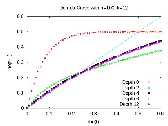
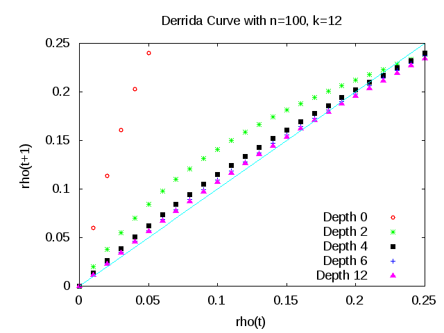
Figure 1: Derrida curves for random Boolean networks with $n=100$ nodes and $k=12$ inputs per function.

The Derrida curves corresponding to networks constructed using functions of larger depth show more orderly dynamics than those of smaller depth. This reaffirms the idea in [18] that sensitivity of a function is an indicator of the dynamical stability of networks constructed with these functions. The curves move closer together as the depth increases. For example, the depth-$2$ networks are much more stable than the depth-$0$ networks, and networks with functions of depth at least $4$ are even more stable; however, the marginal benefit of stability as depth increases drops off sharply – the Derrida curves are nearly identical for networks with functions of depth $4$, $6$, $8$, $10$, and $12$. This matches our theoretical results of Theorem 2 on expected activities and sensitivities and illustrates how the earlier canalyzing variables have a much greater influence. It also suggests that there is little benefit in imposing the full nested canalyzing structure in network models, as functions with large enough canalyzing depth exhibit very similar stability results without the rigidity of being fully nested canalyzing. Additionally, for small values of $\rho(t)$, the curves quickly approach the line $y=x$ from above, indicating that these networks rapidly move from the chaotic phase toward the critical phase. This is contrary to the claim of [10] that networks comprised of canalyzing functions are always in the frozen phase, but it is in alignment with recent findings of [16] which also refute Kauffuman’s claim, accrediting his results to his choice in parametrization.

6 Concluding Remarks

Canalyzing and nested canalyzing functions have been proposed as gene network models because they exhibit biologically relevant properties. While it is reasonable to expect some Boolean models to have functions with some degree of nested canalyzation, fitting biological data to fully nesting canalyzing functions can be at times artificial, and at other times simply incorrect. Our analysis of the depth that a function retains a canalyzing structure elucidates the role of canalyzation in the dynamics of networks over these functions. Our results on the structure of PNCFs generalize known results on NCFs, and our results on the activities and sensitivities of variables in functions of a given depth generalize similar theorems of simple canalyzing functions. Moreover, we saw that in random Boolean networks, the stability increases with canalyzing depth. However, the marginal gain in stability drops off quickly, in that the stability of our networks with functions of depth at least $d=\frac{k}{3}$ were nearly identical to those with full depth $d=k$. Additionally, just a few degrees of canalyzation are necessary to drop the network into the critical regime, in which many real networks are believed to exist. Together, this suggests that using NCFs in biological models for stability reasons is not only at times rather contrived, but simply unnecessary.

References

- [1] R. Albert and H. Othmer. The topology of the regulatory interactions predicts the expression pattern of the segment polarity genes in Drosophila melanogaster. J. Theor. Bio., 223:1–18, 2003.
- [2] E. Balleza, E. Alvarez-Buylla, A. Chaos, S. A. Kauffman, I. Shmulevich, and M. Aldana. Critical dynamics in genetic regulatory networks: Examples from four kingdoms. PLoS ONE, 3(6):e2456, 2008.
- [3] B. Derrida and Y. Pomeau. Random networks of automata: a simple annealed approximation. Europhys. Lett., 1:45–49, 1986.
- [4] B. Drossel. Random Boolean Networks, chapter 3, pages 69–110. Wiley-VCH Verlag GmbH & Co., Weinheim, Germany, 2009.
- [5] A. Gambin, S. Lasota, and M. Rutkowski. Analyzing stationary states of gene regulatory network using petri nets. Silico Biol., 6:93–109, 2006.
- [6] A. S. Jarrah, B. Raposa, and R. Laubenbacher. Nested canalyzing, unate cascade, and polynomial functions. Physica D, 233:167–174, 2007.
- [7] F. Karlssona and M. Hörnquist. Order or chaos in Boolean gene networks depends on the mean fraction of canalizing functions. Physica A, 384:747–757, 2007.
- [8] S. A. Kauffman. Metabolic stability and epigenesis in randomly constructed genetic nets. J. Theor. Biol., 22(3):437–467, 1969.
- [9] S. A. Kauffman. The Origins of Order: Self-Organization and Selection in Evolution. Oxford Universiy Press, 1993.
- [10] S. A. Kauffman, C. Peterson, B. Samuelsson, and C. Troein. Random Boolean network models and the yeast transcriptional network. Proc. Natl. Acad. Sci., 100(25):14796–9, 2003.
- [11] S. A. Kauffman, C. Peterson, B. Samuelsson, and C. Troein. Genetic networks with canalyzing Boolean rules are always stable. Proc. Natl. Acad. Sci., 101(49):17102–17107, 2004.
- [12] F. Li, T. Long, Y. Lu, Q. Ouyang, and C. Tang. The yeast cell-cycle network is robustly designed. Proc. Natl. Acad. Sci., 11:4781–4786, 2004.
- [13] S. Nikolajewa, M. Friedel, and T. Wilhelm. Boolean networks with biologically relevant rules show ordered behavior. Biosystems, 2006.
- [14] M. Nykter, N. D. Price, M. Aldana, S. A. Ramsey, S. A. Kauffman, L. E. Hood, O. Yli-Harja, and I. Shmulevich. Gene expression dynamics in the macrophage exhibit criticality. Proc. Natl. Acad. Sci., 105:1897–1900, 2008.
- [15] M. Nykter, N. D. Price, A. Larjo, T. Aho, S. A. Kauffman, O. Yli-Harja, and I. Shmulevich. Critical networks exhibit maximal information diversity in structure-dynamics relationships. Phys. Rev. Lett., 100:058702, 2008.
- [16] T. P. Peixoto. The phase diagram of random Boolean networks with nested canalizing functions. Eur. Phys. J. B, 78(2):187–192, 2010.
- [17] J. Saez-Rodriguez, L. Simeoni, J. Lindquist, R. Hemenway, U. Bommhardt, B. Arndt, U. Haus, R. Weismantel, E. Gilles, S. Klamt, and B Schraven. A logical model provides insights into T cell receptor signaling. PLoS Comput. Biol., 3:e163, 2007.
- [18] I. Shmulevich and S. A. Kauffman. Activities and sensitivities in Boolean network models. Phys. Rev. Lett., 93(4):048701, 2004.
- [19] I. Shmulevich, S. A. Kauffman, and M. Aldana. Eukaryotic cells are dynamically ordered or critical but not chaotic. Proc. Natl. Acad. Sci., 102:13439–13444, 2005.
- [20] C. H. Waddington. Canalisation of development and the inheritance of acquired characters. Nature, 150:563–564, 1942.