Computing the local pressure in molecular dynamics simulations

Abstract

Computer simulations of inhomogeneous soft matter systems often require accurate methods for computing the local pressure. We present a simple derivation, based on the virial relation, of two equivalent expressions for the local (atomistic) pressure in a molecular dynamics simulation. One of these expressions, previously derived by other authors via a different route, involves summation over interactions between particles within the region of interest; the other involves summation over interactions across the boundary of the region of interest. We illustrate our derivation using simulations of a simple osmotic system; both expressions produce accurate results even when the region of interest over which the pressure is measured is very small.

1 Introduction

Molecular dynamics (MD) simulations are widely used to study spatially inhomogeneous soft matter systems. In such simulations, it is often necessary to compute the local pressure in a small region of the simulation box, containing only a few atoms or molecules. Examples include calculations of interfacial free energies [1], measurements of osmotic pressure gradients [2, 3] and tests of coarse-grained hydrodynamic theories [4]. While accurate expressions for the local pressure exist, their derivation is rather involved. In this paper, we present a much simpler derivation, which leads to two equivalent expressions for the local pressure. One of these expressions is analogous to the local stress tensor of Lutsko [5] and Cormier et al. [6]; the other is, to our knowledge, new, but is similar in spirit to the “Method of Planes” of Irving and Kirkwood [7] and Todd et al. [8]. We show that both these expressions give accurate results for the local pressure in soft matter systems, even when computed over very small spatial regions.

2 Background

For a spatially homogeneous, closed system, the pressure is commonly computed by taking the average of an instantaneous “pressure function”:

$$P=\langle{\mathcal{P}}\rangle=\left\langle\frac{Nk_{B}T}{V}+\frac{1}{3V}\sum_{i=1}^{N-1}\sum_{j>i}\vec{r}_{ij}\cdot\vec{f}_{ij}\right\rangle$$ (1)

where $N$, $V$ and $T$ are the number of particles, volume and temperature, $k_{B}$ is Boltzmann’s constant, $\vec{r}_{i}$ and $\vec{r}_{j}$ are the positions of particles $i$ and $j$, $\vec{r}_{ij}\equiv\vec{r}_{i}-\vec{r}_{j}$, and $\vec{f}_{ij}$ denotes the force exerted on particle $i$ by particle $j$ [9, 10]; the double sum runs over all pairs of particles, avoiding double counting. The first and second terms in Eq.(1) arise from the kinetic energy of the particles and from interparticle interactions, respectively. Expression (1) can be derived in a few steps starting from the Clausius virial relation

$$\left\langle\sum_{i=1}^{N}\frac{|\vec{p}_{i}|^{2}}{m_{i}}+\sum_{i=1}^{N}\vec{r}_{i}\cdot\vec{F}_{i}\right\rangle=0,$$ (2)

in which $\vec{p}_{i}$ and $m_{i}$ are the momentum and mass of particle $i$, and $\vec{F}_{i}$ is the total force acting on particle $i$, due to other particles and the walls of the container [11, 12].

For spatially inhomogeneous systems, one can measure directly the pressure across a local plane within the simulation box via the “method of planes” (MOP), first proposed by Irving and Kirkwood [7] and later rederived by Todd et al. [8]; this works well when the plane over which the pressure is computed is large, but leads to poor statistical sampling when computing the local pressure in a small region (i.e. over a small plane). Alternatively, the pressure in a local region of interest can be measured using a local version of Eq.(1). This has the advantage that the region of interest can (in principle) be of arbitrary shape, and that statistical averages are taken over a volume rather than an area. The following local pressure function was proposed by Lutsko [5] and later reformulated by Cormier et al. [6] (note that these authors considered the full stress tensor, while, for simplicity, we focus only on the scalar pressure, which we assume to be locally isotropic):

$$P(\vec{r})=\frac{1}{3\Omega}\left\langle\sum_{i=1}^{N}\frac{|p_{i}|^{2}}{m_{i}}\Lambda_{i}+\sum_{i=1}^{N-1}\sum_{j>i}(\vec{f}_{ij}\cdot\vec{r}_{ij})l_{ij}\right\rangle.$$ (3)

Here, $\Omega$ is the volume of the region of interest, centred on $\vec{r}$, $\Lambda_{i}$ is unity if particle $i$ lies within the volume $\Omega$, and zero otherwise, and $l_{ij}$ is the fraction ($0\leq l_{ij}\leq 1$) of the line joining particles $i$ and $j$ that lies within $\Omega$ (see Figure 1). The local pressure expression (3) is analogous to the global one (1), but with two important differences. Firstly, in the kinetic part of Eq.(3), only those particles which are inside the region of interest (at time $t$) are included. Secondly, the components of the interaction term are weighted by the fraction of the line joining particles $i$ and $j$ that is inside the region of interest; this highlights the crucial importance of correctly accounting for interparticle interactions which cross the boundary of the region of interest. Note that particles $i$ and $j$ may both be outside the region yet still contribute to the interaction pressure; see Figure 1.

Figure 1: Contributions to the interaction part of Eq.(3) from different pairs of particles: the fraction $l_{ij}$ of the line joining particles $i$ and $j$ which lies inside the region of interest is shown as a solid line. $\vec{b}_{ij}$ denotes the position where the line joining particles $i$ and $j$ crosses the boundary.

Both Lutsko [5] and Cormier et al. [6] derive the stress tensor version of Eq.(3) by Fourier transforming the continuity equation for the local momentum flux and applying Newton’s second law. In this paper, we present a simpler and arguably more intuitive, real space derivation, which is directly analogous to the derivation of the global pressure expression, Eq.(1), from the Clausius virial relation (2). This derivation leads both to Eq.(3) and to a new expression for the local pressure involving the flux of particle momentum across the boundaries of the region of interest, together with cross-boundary interactions. The equivalence between these two expressions shows directly how the relation between surface flux and volume pressure measurements extends to the atomic scale. Our approach may also prove useful in future for deriving local pressure expressions for systems with different dynamical rules, such as run-and-tumble swimmers [13] or particles with viscous dynamics [10].

3 Derivation of expressions for the local pressure

To compute the local pressure at some position $\vec{r}$ in the system, we consider a local region of fluid, of volume $\Omega$, centred on $\vec{r}$. Particles within this region interact with other particles both inside and outside the region. During a given time interval, particles will enter and leave the region of interest.

3.1 The Schweitz virial relation

We begin with an analogue of the Clausius virial relation (2), derived by Schweitz, for open systems [14]. The Schweitz virial relation states that

$$\left\langle\sum_{i=1}^{N}\frac{|\vec{p}_{i}|^{2}}{m_{i}}\Lambda_{i}(\vec{r})+\sum_{i=1}^{N}\vec{r}_{i}\cdot\left(\sum_{j\neq i}\vec{f}_{ij}\right)\Lambda_{i}(\vec{r})+\sum_{i=1}^{N}\left(\vec{r}_{i}\cdot\vec{p}_{i}\right)\dot{\Lambda_{i}}\right\rangle=0,$$ (4)

where, as above, the function $\Lambda_{i}(t)$ measures whether or not particle $i$ is within the region of interest at time $t$, and its time derivative $d\Lambda_{i}(t)/dt\equiv\dot{\Lambda_{i}}$ produces a positive or negative $\delta$-function peak at the moment when particle $i$ enters or leaves the region of interest . The first term in Eq.(4), $\left\langle\sum_{i=1}^{N}\frac{|\vec{p}_{i}|^{2}}{m_{i}}\Lambda_{i}(\vec{r})\right\rangle\equiv E_{kin}$, is the average kinetic energy of particles in the region of interest and is directly analogous to the first term in Eq.(2). The second, interaction, term is analogous to the second term in Eq.(2) – we assume that there are no external forces so the total force on particle $i$ is given by the sum of interactions with all other particles in the system. The final term in Eq.(4), $\left\langle\sum_{i=1}^{N}\left(\vec{r}_{i}\cdot\vec{p}_{i}\right)\dot{\Lambda_{i}}\right\rangle\equiv\Phi$, accounts for the exchange of particles between the region of interest and its surroundings. Particles entering the region contribute $\vec{r}_{i}\cdot\vec{p}_{i}$ while those leaving contribute $-\vec{r}_{i}\cdot\vec{p}_{i}$; these do not cancel because the momentum vectors $\vec{p}_{i}$ for particles entering and leaving are opposite in sign.

We now split the second term in Eq.(4) into contributions due to interactions with particles inside and outside the region of interest:

$$\sum_{i=1}^{N}\vec{r}_{i}\cdot\left(\sum_{j\neq i}\vec{f}_{ij}\right)\Lambda_{i}(\vec{r})=\mathcal{V}_{int}+\mathcal{V}_{ext},$$ (5)

where $\mathcal{V}_{int}\equiv\left\langle\sum_{i=1}^{N}\sum_{j\neq i}\vec{r}_{i}\cdot\vec{f}_{ij}\,\,\Lambda_{i}\Lambda_{j}\right\rangle=\left\langle\sum_{i=1}^{N-1}\sum_{j>i}\vec{r}_{ij}\cdot\vec{f}_{ij}\,\,\Lambda_{i}\Lambda_{j}\right\rangle\equiv\left\langle\sum_{\mathrm{in\,in}}\vec{r}_{ij}\cdot\vec{f}_{ij}\right\rangle$ contains contributions where both particles are inside the region of interest and $\mathcal{V}_{ext}\equiv\left\langle\sum_{i=1}^{N}\sum_{j\neq i}\vec{r}_{i}\cdot\vec{f}_{ij}\,\,\Lambda_{i}(1-\Lambda_{j})\right\rangle\equiv\left\langle\sum_{\mathrm{in\,out}}\vec{r}_{i}\cdot\vec{f}_{ij}\right\rangle$ contains contributions where particle $i$ is inside the region and particle $j$ is outside. Substituting Eq.(5) into Eq.(4) allows us to write the Schweitz virial relation as

$$E_{kin}+\mathcal{V}_{int}+\mathcal{V}_{ext}+\Phi=0.$$ (6)

3.2 Expressions for the local pressure

We next use the Schweitz virial relation to derive expressions for the local pressure. The local pressure has two components: a kinetic component, $P_{kin}(\vec{r})$, which is given by the normal flux of particle momentum across the boundaries of the region of interest and an interaction component, $P_{int}(\vec{r})$, which is the surface density of interparticle forces across the boundary. Throughout this paper the normal to the boundary is assumed to point in the outward direction.

Kinetic component

The kinetic component of the local pressure can be related to the component $\Phi\equiv\left\langle\sum_{i=1}^{N}\left(\vec{r}_{i}\cdot\vec{p}_{i}\right)\dot{\Lambda_{i}}\right\rangle$ of the Schweitz virial relation. To see this, we split the particle momentum, $\vec{p}_{i}$, into its components normal and tangential to the boundary: $\vec{p}_{i}=(\vec{p}_{i}\cdot\hat{n})\hat{n}+(\vec{p}_{i}\cdot\hat{t})\hat{t}$, to give

$$\Phi=\left\langle\sum_{i=1}^{N}\dot{\Lambda_{i}}\left[(\vec{p}_{i}\cdot\hat{n})(\vec{r}_{i}\cdot\hat{n})+(\vec{p}_{i}\cdot\hat{t})(\vec{r}_{i}\cdot\hat{t})\right]\right\rangle.$$ (7)

Assuming that the density of particles is uniform across the region of interest, the second term in Eq.(7) averages to zero. Next, we notice that because $\dot{\Lambda_{i}}$ is nonzero only when a particle is at the boundary, $\vec{r}_{i}\cdot\hat{n}$ may be taken outside the summation. Assuming (without loss of generality) that the region of interest is cubic with the origin at its centre and sides of length $L$, $\vec{r}_{i}\cdot\hat{n}=L/2$, and the total (outward) momentum flux $\left\langle\sum_{i}(\vec{p}_{i}\cdot\hat{n})\dot{\Lambda_{i}}\right\rangle$ across each of the 6 faces is $-P_{kin}L^{2}$. Eq.(7) therefore reduces to

$$\Phi=-3\Omega P_{kin}(\vec{r}).$$ (8)

Interaction component

In a similar way, the interaction component of the local pressure, $P_{int}(\vec{r})$, can be related to the component $\mathcal{V}_{ext}$ of the Schweitz virial relation. We first note that the position vector $\vec{r}_{i}$ may be written as $\vec{r}_{i}=\vec{b}_{ij}+\vec{r}_{ij}l_{ij}$, where $\vec{b}_{ij}$ denotes the position where the line linking particles $i$ and $j$ crosses the boundary of the region of interest, and $l_{ij}$ is the fraction of the line linking particles $i$ and $j$ that lies inside the region of interest (see Figure 1). $\mathcal{V}_{ext}$ is then given by

$$\mathcal{V}_{ext} = \left\langle\sum_{\mathrm{in\,out}}\vec{b}_{ij}\cdot\vec{f}_{ij}+l_{ij}\left(\vec{r}_{ij}\cdot\vec{f}_{ij}\right)\right\rangle$$

$$= \left\langle\sum_{\mathrm{in\,out}}(\vec{f}_{ij}\cdot\hat{n})\left(\vec{b}_{ij}\cdot\hat{n}\right)\right\rangle+C_{t}+\left\langle\sum_{\mathrm{in\,out}}l_{ij}\left(\vec{r}_{ij}\cdot\vec{f}_{ij}\right)\right\rangle,$$

where the second line follows from splitting the interparticle force $\vec{f}_{ij}$ into its components normal and tangential to the boundary: $\vec{f}_{ij}=(\vec{f}_{ij}\cdot\hat{n})\hat{n}+(\vec{f}_{ij}\cdot\hat{t})\hat{t}$, and $C_{t}=\left\langle\sum_{\mathrm{in\,out}}(\vec{f}_{ij}\cdot\hat{t})\left(\vec{b}_{ij}\cdot\hat{t}\right)\right\rangle$. Focusing on the first term, we note that $\vec{b}_{ij}$ points to the boundary and so (assuming the same cubic geometry as above), $\vec{b}_{ij}\cdot\hat{n}=L/2$. Denoting as $\sigma$ the average outward normal force per unit area crossing the boundary, due to the $(i\,{\mathrm{in}},j\,{\mathrm{out}})$ interactions, we obtain

$$\left\langle\sum_{\mathrm{in\,out}}(\vec{f}_{ij}\cdot\hat{n})\left(\vec{b}_{ij}\cdot\hat{n}\right)\right\rangle=-6\left(\frac{L}{2}\right)(L^{2}\sigma)=-3\Omega\sigma.$$ (10)

The interaction component of the pressure, $P_{int}(\vec{r})$, is equal to the total surface density of normal force crossing the boundary: $P_{int}=\sigma+\xi$, where $\xi$ is the normal contribution due to pairs of particles $i$ and $j$ which are both outside the region of interest (see Figure 1). We demonstrate in the Appendix that

$$-3\Omega\xi=C_{t}-\left\langle\sum_{\mathrm{out\,out}}l_{ij}\left(\vec{r}_{ij}\cdot\vec{f}_{ij}\right)\right\rangle$$ (11)

so that, putting together Eqs(3.2)-(11), we can relate $P_{int}$ to $\mathcal{V}_{ext}$ by:

$$-3\Omega P_{int}(\vec{r}) = -3\Omega(\sigma+\xi)=\mathcal{V}_{ext}-\mathcal{V}_{corr},$$ (12)

where

$$\mathcal{V}_{corr}\equiv\left\langle\sum_{\mathrm{in\,out}}l_{ij}\left(\vec{r}_{ij}\cdot\vec{f}_{ij}\right)+\sum_{\mathrm{out\,out}}l_{ij}\left(\vec{r}_{ij}\cdot\vec{f}_{ij}\right)\right\rangle.$$ (13)

“Boundary” expression for the local pressure

An expression for the local pressure, $P(\vec{r})$, can be obtained by combining Eqs.(8) and (12):

$$P(\vec{r}) = P_{kin}+P_{int}=-\frac{1}{3\Omega}\left[\Phi+\mathcal{V}_{ext}-\mathcal{V}_{corr}\right]$$

$$= -\frac{1}{3\Omega}\left[\left\langle\sum_{i=1}^{N}\left(\vec{r}_{i}\cdot\vec{p}_{i}\right)\dot{\Lambda_{i}}+\sum_{\mathrm{in\,out}}\left(\vec{r}_{i}-l_{ij}\vec{r}_{ij}\right)\cdot\vec{f}_{ij}-\sum_{\mathrm{out\,out}}l_{ij}\vec{r}_{ij}\cdot\vec{f}_{ij}\right\rangle\right].$$

Eq.(3.2) provides a simple prescription for computing the local pressure. The first term sums over all particles which enter or leave the region of interest and is equivalent to the momentum flux density due to particles crossing the boundary, while the remaining terms, which account for the force density at the boundary due to interparticle interactions, sum over all pairs of particles for which the line connecting the two particles crosses the boundary of the region of interest. In the case where the region of interest is large, $P(\vec{r})$ is dominated by the contributions of $\Phi$ and $\mathcal{V}_{ext}$ ($\mathcal{V}_{corr}$ becomes negligible); however, as we show below in Figure 2, $\mathcal{V}_{corr}$ makes an important contribution when the region of interest is small. Eq.(3.2) provides an alternative to existing local pressure expressions, and demonstrates explicitly how the relation between surface flux and volume pressure expressions extends to very small regions of space.

“Volume” expression for the local pressure

The Schweitz virial relation provides a direct route from this “boundary” expression to the more usual expression for the local pressure, which involves a sum over particles within the region of interest. Inserting Eq.(3.2) into the Schweitz relation (6), we obtain:

$$P(\vec{r})=\frac{1}{3\Omega}\left[E_{kin}+\mathcal{V}_{int}+\mathcal{V}_{corr}\right]$$

$$= \frac{1}{3\Omega}\left\langle\sum_{i=1}^{N}\frac{|\vec{p}_{i}|^{2}}{m_{i}}\Lambda_{i}(\vec{r})+\sum_{\mathrm{in\,in}}\vec{r}_{ij}\cdot\vec{f}_{ij}+\sum_{\mathrm{in\,out}}l_{ij}\left(\vec{r}_{ij}\cdot\vec{f}_{ij}\right)+\sum_{\mathrm{out\,out}}l_{ij}\left(\vec{r}_{ij}\cdot\vec{f}_{ij}\right)\right\rangle$$

$$= \frac{1}{3\Omega}\left\langle\sum_{i=1}^{N}\frac{|\vec{p}_{i}|^{2}}{m_{i}}\Lambda_{i}(\vec{r})+\sum_{i}\sum_{j>i}l_{ij}\left(\vec{r}_{ij}\cdot\vec{f}_{ij}\right)\right\rangle,$$

where the last line follows from the fact that $l_{ij}=1$ if both particles are inside the region of interest (assuming the boundary is everywhere concave). Eq.(3) is identical to Eq.(3), and constitutes a local version of the global instantaneous pressure function, Eq.(1).

4 Molecular dynamics simulations

We now illustrate, using molecular dynamics simulations, the Schweitz virial relation (6) as well as the two expressions for the local pressure, Eqs.(3.2) and (3). In our simulations, a periodic box contains 5000 particles at a density $\rho=0.8$ (reduced units [10]), which interact via a repulsive Weeks, Chandler, Andersen (WCA) potential [15] (a truncated and shifted Lennard-Jones potential). The particle size $\sigma=1$, the interaction parameter $\epsilon=1$ (both in reduced units) and the box length is $18.42\sigma$. The system is simulated using the velocity Verlet algorithm [10] with timestep $\Delta t=0.001$ (reduced units) and is maintained in the canonical (NVT) ensemble using a Nosé-Hoover thermostat at temperature, $T=1.0$ (reduced units). All runs are equilibrated for $4\times 10^{4}$ timesteps prior to data collection, and data is collected over at least $2\times 10^{6}$ timesteps. Errors are computed using bootstrapping [16], with 1000 replica datasets.

4.1 A homogeneous fluid

We first consider a homogeneous fluid, for which the local pressure, measured using Eqs.(3.2) and (3), should match the global pressure, measured using Eq.(1). We define a cubic region of interest, located in the centre of our simulation box, whose size $L$ we vary from $L=5.5\sigma$ to $L=3\sigma$. For this smallest value of $L$, the region of interest contains only $\sim 21$ particles on average.

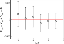
(a)          (b)

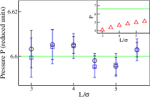
Figure 2: Molecular dynamics simulation results for the homogeneous fluid. (a): $E_{kin}+\mathcal{V}_{int}+\mathcal{V}_{ext}+\Phi$ as a function of the size $L$ of the region of interest. (b): Local pressure in the region of interest, computed using Eq.(3.2) (blue squares) and Eq.(3) (black circles). The apparent correlation between these results arises because the same simulation data set was used in both cases. The green line shows the global pressure computed using Eq.(1). The inset shows the pressure computed using Eq.(3), not including $\mathcal{V}_{corr}$ (red triangles; note the very different scale on the pressure axis).

Figure 2a shows $E_{kin}+\mathcal{V}_{int}+\mathcal{V}_{ext}+\Phi$ as a function of the size $L$ of the region of interest. As predicted by the Schweitz virial relation (6), this quantity is zero within our error bars (note that of the individual terms in this sum, two are $\sim$ 5 and the other two are $\sim$ 0.8). Figure 2b shows the local pressure $P(\vec{r})$ in the region of interest, computed using expressions (3.2) and (3), as a function of $L$. Both expressions give results in excellent agreement with the global pressure across the whole simulation box, using Eq.(1). The inset to Figure 2b, which shows Eq.(3), neglecting the $\mathcal{V}_{corr}$ term, demonstrates the importance of correctly accounting for the boundary terms: neglecting $\mathcal{V}_{corr}$ gives a large error, which increases as $L$ decreases.

4.2 An osmotic system

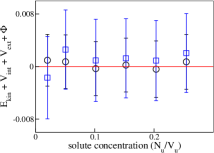
(a)          (b)

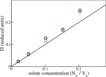
Figure 3: Molecular Dynamics simulations for the osmotic system. (a): $E_{kin}+\mathcal{V}_{int}+\mathcal{V}_{ext}+\Phi$, as a function of the concentration $N_{u}/V_{u}$ of solute particles, computed for a small subregion (of dimensions $L_{x}=L_{y}=L_{z}=6\sigma$) within the solution region (black circles) and for a small subregion ($L_{x}=2\sigma$, $L_{y}=L_{z}=7\sigma)$ outside the solution (blue squares). (b): Osmotic pressure difference $\Pi$ between the solution and its surroundings, computed using Eq.(3.2) (green triangles) and using Eq.(3) (blue circles) (for the same subregions). Results are also shown for a direct computation of the normal solute-membrane force per unit area (red squares). Error bars are smaller than the symbols. The prediction of the van’t Hoff equation, $\Pi=(N_{u}k_{B}T)/V_{u}$, is also shown (black line).

We next consider an osmotic system, in which the local pressure differs in different parts of the simulation box. To construct this system we label a subset $N_{u}$ of the particles “solute” and the remaining particles “solvent”. Solute particles are confined to a cubic region of volume $V_{u}\approx 786\sigma^{3}$ in the center of the simulation box by a smooth confining potential; solvent particles do not experience this potential and are free to move throughout the simulation box. The confining potential acts as a semi-permeable membrane, resulting in an osmotic pressure difference, $\Pi$, between the “solution” region where the solutes are confined and the rest of the simulation box.

To compute the osmotic pressure, we define local regions of interest inside and outside the solution compartment (for dimensions see the caption of Figure 3). Figure 3a shows that the Schweitz virial relation (6) is obeyed in both of these local regions, over a range of solute concentrations. The pressure in the two local regions can be computed using Eqs. (3.2) and (3); subtracting the results gives the osmotic pressure difference, $\Pi$. Figure 3b shows $\Pi$, as a function of the concentration $N_{u}/V_{u}$ of solute particles in the solution compartment; both methods for computing the local pressure produce results in excellent agreement with a direct calculation of the osmotic pressure obtained by measuring the average confining force on the solutes, per unit area of the confining box.

5 Conclusions

Accurate methods for computing the local pressure are essential for simulating inhomogeneous soft matter systems. In this paper, we have derived two equivalent expressions for the local pressure in a molecular dynamics simulation. The “boundary” expression, Eq.(3.2), is, to our knowledge, new. This expression involves summation over interactions between particles within and outside the local region of interest and is similar in spirit to the “method of planes” approach of Irving and Kirkwood [7] and of Todd et al. [8]. The “volume” expression Eq.(3) is a local analogue of the function commonly used to compute the global pressure in homogeneous simulations; this involves summation over interactions between pairs of particles within the region of interest. This expression was previously derived via a Fourier transform method by Lutsko [5] and by Cormier et al. [6]; our derivation, based on the Schweitz virial relation, provides a simple real-space alternative. Importantly, both local pressure expressions take careful account of interactions close to the boundary: this is crucial when the region of interest is of the order of the particle size.

The derivation presented in this paper, via the Schweitz virial relation, demonstrates explicitly how the equivalence between surface flux and volume expressions for the pressure, familiar from macroscopic systems, plays out on very small (atomistic) lengthscales. This approach may also prove useful in future for deriving local pressure expressions in systems whose dynamics are more complex: for example systems with viscous dynamics [10], or active matter systems in which particles are self-propelled and/or chemotactic [13]. Here, the Fourier transform method of Lutsko and Cormier et al. [5, 6] might prove challenging, but we hope that our real-space method should hold with only minor modifications.

Finally, we note that an important assumption made in this work is that the local pressure is isotropic: we therefore derive expressions for the scalar pressure rather than the local pressure tensor, as in previous work [5, 6, 7, 8]. We believe that it should be possible to extend the present derivation to obtain the analogous expressions for the pressure tensor, via a tensor analogue of the Schweitz virial relation. For the present, we leave this as an interesting avenue for future work.

Appendix: Pairs of particles which are both outside the region of interest

Here, we discuss the contribution to the interaction component of the pressure made by pairs of particles $i$ and $j$, in the cases where both particles are outside the region of interest, but (as illustrated in Figure 1), the line joining particles $i$ and $j$ crosses the boundary. Our aim is to derive Eq.(11). Assuming that the region of interest is cubic (with side length $L$ and origin at the centre), the line joining particles $i$ and $j$ crosses the boundary on two different faces. We define these crossing points by the position vectors $\vec{b}_{ij}^{(1)}$ and $\vec{b}_{ij}^{(2)}$. Figure 4a illustrates that $l_{ij}\vec{r}_{ij}=\vec{b}_{ij}^{(2)}-\vec{b}_{ij}^{(1)}$. This allows us to write

$$\left\langle\sum_{\mathrm{out\,out}}l_{ij}\left(\vec{r}_{ij}\cdot\vec{f}_{ij}\right)\right\rangle=\left\langle\sum_{\mathrm{out\,out}}\left(\vec{b}_{ij}^{(2)}\cdot\vec{f}_{ij}\right)-\left(\vec{b}_{ij}^{(1)}\cdot\vec{f}_{ij}\right)\right\rangle.$$ (16)

We now resolve $\vec{b}_{ij}^{(1)}$ and $\vec{b}_{ij}^{(2)}$ into components normal and tangential to the boundary on faces 1 and 2 respectively [$\vec{b}_{ij}^{(1)}=(\vec{b}_{ij}^{(1)}\cdot\hat{n}^{(1)})\hat{n}^{(1)}+(\vec{b}_{ij}^{(1)}\cdot\hat{t}^{(1)})\hat{t}^{(1)}$ etc]. Noting that $(\vec{b}_{ij}^{(1)}\cdot\hat{n}^{(1)})=(\vec{b}_{ij}^{(2)}\cdot\hat{n}^{(2)})=L/2$, we obtain

$$\left\langle\sum_{\mathrm{out\,out}}l_{ij}\left(\vec{r}_{ij}\cdot\vec{f}_{ij}\right)\right\rangle=3\Omega\xi-(D_{t}^{(1)}+D_{t}^{(2)}),$$ (17)

where $\xi$ is the (outward) normal force per unit area crossing the boundary due to particle pairs which are both outside the region of interest, $D_{t}^{(1)}=\left\langle\sum_{\mathrm{out\,out}}(\vec{b}_{ij}^{(1)}\cdot\hat{t}^{(1)})(\vec{f}_{ij}\cdot\hat{t}^{(1)})\right\rangle$ and $D_{t}^{(2)}=\left\langle\sum_{\mathrm{out\,out}}(\vec{b}_{ij}^{(2)}\cdot\hat{t}^{(2)})(\vec{f}_{ji}\cdot\hat{t}^{(2)})\right\rangle$ (we use $\vec{f}_{ji}=-\vec{f}_{ij}$). Assuming that particles are homogeneously distributed across the region of interest, $D_{t}^{(1)}=D_{t}^{(2)}=D_{t}/2$ (by symmetry, see Figure 4a).

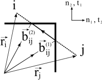
(a)           (b)

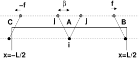
Figure 4: (a) Geometric illustration of the case where particles $i$ and $j$ are both outside the region of interest. (b) Illustration of the simplified one dimensional scenario used to show that $C_{t}=-D_{t}$.

We now demonstrate that $D_{t}=-C_{t}$, where $C_{t}$, as defined in Section 3, is the tangential component of the ($i\,{\mathrm{in}},j\,{\mathrm{out}}$) contribution to $\mathcal{V}_{ext}$. We study the simplified one dimensional scenario shown in Figure 4b, in which we consider only particles $i$ and $j$ lying along two lines parallel to the $x$ axis. We further assume that interactions are restricted in range, such that each particle $i$ interacts with only two interaction partners $j$, as shown in Figure 4b, with tangential forces $f$ in opposite directions. These interactions contribute respectively $f(x_{i}-\beta)$ and $-f(x_{i}+\beta)$ to the sum $\sum_{i}\sum_{j}(\vec{b}_{ij}\cdot\hat{t})(\vec{f}_{ij}\cdot\hat{t})$. We now sum the contribution of the interactions shown in Figure 4b for the cases where particle $i$ is inside the region of interest ($-L/2<x_{i}<L/2$) and the line joining $i$ and $j$ crosses the top face of the region – i.e. the contributions to $C_{t}$ for this face. The result is $f\beta d(\beta-L)$, where $d$ is the number of particles $i$ per unit length along the line . Next, we sum the contributions for the cases where particle $i$ is outside the region of interest, but the line joining $i$ and $j$ still crosses the top face of the region (i.e. the contributions to $D_{t}$ for this face). Contributions $\pm(x\mp\beta)f$ are made by particles $i$ for which $(-L/2-\beta)<x_{i}<-L/2$ or $L/2<x_{i}<(L/2+\beta)$ (case C in Figure 4b). Integrating over these ranges of $x_{i}$, we obtain a total contribution to $D_{t}$ of $f\beta d(L-\beta)$. Thus the contributions to the ($i\,{\mathrm{in}},j\,{\mathrm{out}}$) tangential term $C_{t}$ are exactly compensated by the contributions to the ($i\,{\mathrm{out}},j\,{\mathrm{out}}$) tangential term $D_{t}$, and Eq.(17) reduces to Eq.(11).

References

- [1] M. Schrader, P. Virnau, D. Winter, T. Zykova-Timan and K. Binder Eur. Phys. J., 177:103-127, 2009.
- [2] J.-L. Barrat and J.-P. Hansen Basic Concepts for Simple and Complex Fluids Cambridge University Press, 2003.
- [3] T. W. Lion and R. J. Allen (in preparation)
- [4] M. Schindler Chem. Phys., 375:327-336, 2010.
- [5] J. F. Lutsko J. App. Phys., 64:1152–1154, 1988.
- [6] J. Cormier, J. M. Rickman and T. J. Delph J. App. Phys., 89:99–104, 2001.
- [7] J. H. Irving and J. G. Kirkwood J. Chem. Phys., 18:817–829, 1950.
- [8] B. D. Todd, D. J. Evans and P. J. Daivis Phys. Rev. E, 52:1627–1638, 1995.
- [9] P. S. Y. Cheung Mol. Phys., 33:519–526, 1977.
- [10] M. P. Allen and D.J. Tildesley Computer Simulation of Liquids Oxford University Press, 1992.
- [11] R. Clausius The London, Edinburgh and Dublin Philosophical Magazine and Journal of Science, 40:122–127, 1870.
- [12] J. J. Erpenbeck and W. W. Wood in B. J. Berne, ed. Modern theoretical chemistry Plenum, New York, 1977, vol 6B.
- [13] M. E. Cates Rep. Prog. Phys., 75:042601, 2012.
- [14] J. Schweitz J. Phys. A: Math. Gen., 10:507–515, 1977.
- [15] J. D. Weeks, D. Chandler and H. C. Andersen J. Chem. Phys., 54:5237–5247, 1971.
- [16] B. Efron The Annals of Statistics, 7:1-26, 1979
- [17] J. H. van’t Hoff. Z. Phys. Chem., 1:481–508, 1887.