2.5PN linear momentum flux from inspiralling compact binaries in quasicircular orbits and associated recoil: Nonspinning case

Abstract

Anisotropic emission of gravitational waves (GWs) from inspiralling compact binaries leads to the loss of linear momentum and hence gravitational recoil of the system. The loss rate of linear momentum in the far-zone of the source (a nonspinning binary system of black holes in quasicircular orbit) is investigated at the 2.5 post-Newtonian (PN) order and used to provide an analytical expression in harmonic coordinates for the 2.5PN accurate recoil velocity of the binary accumulated in the inspiral phase. We find that the recoil velocity at the end of the inspiral phase (i.e at the innermost stable circular orbit (ISCO)) is maximum for a binary with symmetric mass ratio of $\nu\sim 0.2$ and is roughly about $\sim$4.58 ${\rm km\,s}^{-1}$. Going beyond inspiral, we also provide an estimate of the more important contribution to the recoil velocity from the plunge phase. Again the recoil velocity at the end of the plunge, involving contributions both from inspiral and plunge phase, is maximum for a binary with $\nu\sim 0.2$ and is of the order of $\sim$180 ${\rm km\,s}^{-1}$.

I Introduction

A coalescing black-hole (BH) binary which is anisotropically emitting gravitational waves (GWs) will experience a recoil as a consequence of the loss of linear momentum from the binary through outgoing GWs. This phenomenon of gravitational-wave recoil has substantial importance in astrophysics especially if one wants to study models which suggest the formation and growth of super massive black holes (SMBHs) at the centers of galaxies through successive mergers from smaller BHs (stellar or intermediate mass BHs) Merritt et al. (2004). If the kick velocity of the product BH is more than its escape velocity from the host galaxy, the formation of SMBHs will not be favored, as would be the case with dwarf galaxies and globular clusters (see Komossa et al. (2008) for observational evidence for ejection of the SMBHs). Even if the recoil velocity of the product BH is not sufficient to eject it from the host (which may be the case with giant elliptical galaxies), the product BH would be displaced from the center and eventually would fall back. Such a process may have important dynamical changes at the galactic core. For a more detailed overview of astrophysical possibilities, see Ref.Merritt et al. (2004). One important claim of Merritt et al. (2004) is that models that grow SMBHs from the mergers of smaller BHs will not be favored for the galaxies at redshifts $\rm{z}\,{\gtrsim}\,10$ due to the difficulty in retaining the “kicked” black holes. However, observations of the local universe suggest that most of the galaxies (more than 50% of them) have SMBHs at their centers Richstone et al. (1998). This shows that there must be something which prevents the ejection of the central black-hole from many of these galaxies and Ref.Schnittman (2007) investigates such questions. In the light of the above arguments it becomes important to have an accurate estimate of the recoil velocity of the coalescing binary black holes (BBHs).

One of the first proposals investigating the phenomenon of gravitational-wave recoil is due to Peres Peres (1962). Following the analogy from the classical electrodynamics, it was suggested that the lowest order secular effects related to gravitational-wave recoil arise due to the interaction of mass quadrupole moment with mass octupole moment or current quadrupole moment. His work provided the first formal theory for gravitational-wave recoil of a general material system in linearized gravity and is valid for any kind of motion (rotational, vibrational or any other kind) given the source is localized within a finite volume. In another early work, Bonnor and Rotenberg Bonnor and Rotenberg (1961) studied the emission of gravitational waves from a pair of oscillating particles and suggested the possibility of GW recoil. Papapetrou Papapetrou (1962) derived the leading order formula which involved interaction of mass quadrupole moment with mass octupole moment and current quadrupole moment. Later, Thorne Thorne (1980) generalized the idea by providing a general multipole expansion for the linear momentum loss as seen in the far zone of the source.

Within the post-Newtonian (PN) scheme, the leading order contribution to the linear momentum flux from an inspiralling binary system of two point masses in Keplarian orbit was computed by Fitchett Fitchett (1983) and binary motion in circular orbit was discussed as a limiting case of the main results of the work. The first PN correction was added to it by Wiseman Wiseman (1992) and the circular orbit case was discussed as a special case. In a work by Blanchet, Qusailah and Will (hereafter BQW) Blanchet et al. (2005) the 1PN expression for linear momentum flux, from a nonspinning compact binary moving in quasicircular orbit, was extended to the 2PN order by adding the hereditary contribution that occurs at 1.5PN order and the instantaneous one occurring at the 2PN order. Kidder Kidder (1995) computed the leading order (spin-orbit) contribution to linear momentum flux for generic orbits and discussed circular orbit effects as a limiting case of his findings. Recently, Racine et al. Racine et al. (2009) extended Kidder’s work by adding higher order spin corrections (spin-orbit terms at 1.5PN order, spin-orbit tail and spin-spin terms at 2PN order). They provided 2PN accurate expression for the linear momentum flux from spinning BBHs in generic orbits. They also specialize to the binary motion in circular orbit and provide estimates for the recoil velocity, accumulated during the inspiral phase, for equal mass binaries with spins equal in magnitude but opposite in direction.

Using the black-hole perturbation theory, Favata et al. Favata et al. (2004) estimated the recoil velocity of the binary, treating it as a test particle inspiralling into a black-hole (spinning or nonspinning), up to the innermost stable circular orbit (ISCO) (accounting for the recoil velocity accumulated during the inspiral phase) very accurately. Though their calculations were valid only in extreme mass ratio limit ($q_{\rm m}\equiv m_{1}/m_{2}<<1$) they extrapolated their results to $q_{\rm m}\sim 0.4$ (with modest accuracy) using some scaling results from quadrupole approximations. A crude estimate of the contributions due to the plunge was also given. Within the validity of the approach, their estimates suggested the typical recoil velocity can be of the order of 10-100 ${\rm km\,s}^{-1}$ but for some configurations it may reach roughly up to 500 ${\rm km\,s}^{-1}$. Another computation by Damour and Gopakumar Damour and Gopakumar (2006) used the effective one-body approach Buonanno and Damour (1999); Damour (2001) to compute the total recoil velocity of the final black-hole taking into account the contributions from all the three phases (inspiral, plunge and ringdown). Depending upon the method they used to compute linear momentum flux their estimates for maximum recoil velocity lie in the range 49-172 ${\rm km\,s}^{-1}$. Reference Sopuerta et al. (2007) presents estimates of the recoil velocities for binaries in orbits with small eccentricities using an approximation technique that is valid only for late stages of the plunge. They also combine their results with the PN estimates of recoil velocity at ISCO of BQW in order to give estimates for recoil velocity for binaries in quasicircular orbits and find that for a binary with symmetric mass ratio (ratio of reduced mass of the binary to the total mass) $\nu=0.2$ the recoil velocity estimates should lie in the range of (79-216) ${\rm km\,s}^{-1}$. In a recent work Le Tiec et al. (2010), the recoil of the final BH was investigated combining the results of Blanchet et al. (2005) with the calculation of contribution from the ringdown phase performed using the close-limit approximation. They found that the radiation emitted in the ringdown phase produces a significant antikick and thus brings down the estimates of recoil velocity based on only inspiral and plunge phase, e.g. after including the contributions from ringdown phase the maximum recoil velocity of the final black-hole is of the order of 180 ${\rm km\,s^{-1}}$ as compared to BQW estimate of 243 ${\rm km\,s^{-1}}$ which does not include the contribution from the ringdown phase (also see Fig.1 of Le Tiec et al. (2010) for a comparison of this result with various numerical and analytical estimates). In another recent work Sundararajan et al. (2010), the phenomenon of recoil of a spinning BBH (extreme mass ratio) due to the inspiral, merger and ringdown phase of its evolution has been investigated. The issue of antikick has been examined very carefully and they found that for orbits aligned with the BH spin, the antikick grows with the spin. Also, a prograde coalescence of a smaller BH into the rapidly rotating bigger BH results in the smallest kick, whereas the retrograde coalescence insures the maximum recoil.

In addition to the analytical or semianalytical estimates of the recoil there have been many investigations using numerical techniques. Recent numerical simulations for nonspinning Campanelli (2005); Baker et al. (2006); Herrmann et al. (2007a); Gonzalez et al. (2009) BBHs in quasicircular orbit have shown that the recoil velocity can reach up to a few hundred ${\rm km\,s}^{-1}$, while for the spinning case Herrmann et al. (2007b); Koppitz et al. (2007); Campanelli et al. (2007); Gonzalez et al. (2007) the recoil velocity estimates are much higher and can be of the order of few thousand ${\rm km\,s}^{-1}$. Although numerical simulations can put better constraints on these estimates, such simulations (especially those which include BH spins) are computationally very expensive. Moreover a very detailed multipolar study of numerical results for BBH recoil Schnittman et al. (2008) shows the need of analytical and semianalytical schemes in order to gain a deeper understanding of the problem at hand and also as a check to numerical results.

In the present work we extend the 2PN calculation of Blanchet et al. (2005) for linear momentum loss from a nonspinning BBH in quasicircular orbit by adding terms (both instantaneous and hereditary) which contribute at 2.5PN order and thus give an analytical expression for linear momentum flux which is now 2.5PN accurate. Naturally, in the 2PN limit our expression for linear momentum flux given by Eq. (29) reduces to Eq. (20) of Blanchet et al. (2005). The 2.5PN accurate expression for the recoil velocity of the binary is given by Eq. (IV) which reduces to Eq. (23) of Blanchet et al. (2005) in the 2PN limit. For computing the contribution to the recoil velocity due to the plunge phase, we simply adopt the discussion given in Sec. (4.1) of Blanchet et al. (2005) and perform the computation using our 2.5PN accurate formulas. We find that the recoil velocity experienced by the binary (with $\nu=0.2$) at the end of inspiral (at fiducial ISCO) and end of the plunge (which includes the contributions from both inspiral and plunge phase) is roughly about $\sim$4.55 ${\rm km\,s}^{-1}$ and $\sim$179.5 ${\rm km\,s}^{-1}$, respectively. In contrast, the recoil velocity at the end of the inspiral and the plunge using the 2PN formulas (see Fig. 1 of Blanchet et al. (2005)) is of the order of 22 ${\rm km\,s}^{-1}$ and 243 ${\rm km\,s}^{-1}$, respectively, corresponding to the same $\nu=0.2$. We see here that inclusion of terms at 2.5PN order brings down the estimates for the recoil velocity significantly, exhibiting in this problem the feature arising from the asymptotic nature of the PN expansion and the need to explicitly investigate the next PN order implications of a calculation. This also reminds us of a similar result of Wiseman (1992) where the inclusion of 1PN contribution brought down the Newtonian estimates since the 1PN term contributed negatively to the recoil velocity. Something similar happens here and the large negative coefficients at 2.5PN order (see Eq. (IV)) brings down the 2PN estimates significantly.

The paper is organized in the following way. In Sec. II, we first provide the PN structure of the linear momentum flux in terms of the radiative multipole moments and then we give explicit expressions for the instantaneous and hereditary contribution separately in terms of the source multipole moments. Section III starts with the formulas for source multipole moments with desired PN accuracy and next shows the computation of both instantaneous and hereditary contributions to the linear momentum in the far-zone of the binary. Finally, we give the 2.5PN accurate expression for the linear momentum flux by adding instantaneous and hereditary contributions. In Sec. IV we discuss the computation of the recoil velocity of the binary and also give the 2.5PN accurate analytical expression for the same. Section V explores the method for estimating the recoil velocity accumulated during the plunge phase. In Sec. VI, we present our numerical estimates of total recoil velocity and its dependence on the composition of the binary as well as final discussions.

II The Post-Newtonian Structure for linear momentum flux

The general formula for linear momentum flux in the far-zone of the source in terms of symmetric trace-free (STF) radiative multipole moments is given in Thorne (1980) and at relative 2.5PN order it takes the following form (see Eq. (4.20)́ of Ref.Thorne (1980).)

$${\mathcal{F}_{P}^{i}}(U) = \frac{G}{c^{7}}\,\biggl{\{}\left[\frac{2}{63}\,U^{(1)}_{ijk}\,U^{(1)}_{jk}+\frac{16}{45}\,\varepsilon_{ijk}U^{(1)}_{ja}\,V^{(1)}_{ka}\right]$$ (1)

$$+{1\over c^{2}}\left[\frac{1}{1134}\,U^{(1)}_{ijkl}\,U^{(1)}_{jkl}+\frac{1}{126}\,\varepsilon_{ijk}U^{(1)}_{jab}\,V^{(1)}_{kab}+\frac{4}{63}\,V^{(1)}_{ijk}\,V^{(1)}_{jk}\right]$$

$$+{1\over c^{4}}\left[\frac{1}{59400}\,U^{(1)}_{ijklm}\,U^{(1)}_{jklm}+\frac{2}{14175}\,\varepsilon_{ijk}U^{(1)}_{jabc}\,V^{(1)}_{kabc}+\frac{2}{945}\,V^{(1)}_{ijkl}\,V^{(1)}_{jkl}\right]+{\cal O}\left({1\over c^{6}}\right)\biggr{\}}.$$

In the above expression $U_{L}$ and $V_{L}$(where $L=i_{1}i_{2}\cdots i_{l}$ represents a multi-index composed of $l$ spatial indices) are the mass-type and current-type radiative multipole moments respectively and $U_{L}^{(p)}$ and $V_{L}^{(p)}$ denote their $p^{\mathrm{th}}$ time derivatives. The Levi-Civita tensor is denoted by $\varepsilon_{ijk}$, such that $\varepsilon_{123}=+1$ and ${\cal O}(1/c^{6})$ indicates that we ignore contributions of the order 3PN and higher. The moments appearing in the formula are functions of retarded time $U\equiv T-({\it R}/c)$ in radiative coordinates. Here $R$ and $T$ denote the distance of the source from the observer and the time of observation in radiative coordinates, respectively.

It should be evident from Eq. (1) that the computation of 2.5PN accurate linear momentum flux requires the knowledge of $U_{ij},V_{ij}$ and $U_{ijk}$ at 2.5PN order, $U_{ijkl}$ and $V_{ijk}$ at 1.5PN order, and $U_{ijklm}$ and $V_{ijkl}$ at Newtonian order. In a recent work Blanchet et al. (2008), $U_{L}$ and $V_{L}$ have been computed with accuracies sufficient for the present purpose using multipolar post-Minkowskian (MPM) approximation approach Blanchet and Faye (2001); Blanchet (2006); Blanchet et al. (2002); Blanchet and Iyer (2005); Blanchet et al. (2004, 2005). In the multipolar post-Minkowskian formalism $U_{L}$ and $V_{L}$ are related to canonical moments $M_{L}$ and $S_{L}$ (Eqs. (5.4)-(5.8) of Blanchet et al. (2008)) which in turn are related to source moments $\left\{I_{L},J_{L},X_{L},W_{L},Y_{L},Z_{L}\right\}$ (Eqs. (5.9)-(5.11) of Blanchet et al. (2008)). Rewriting the expressions for the radiative moments in terms of the source moments, the linear momentum flux can be decomposed as the sum of two distinct parts: the instantaneous terms and the hereditary terms. By instantaneous we refer to contributions in the linear momentum flux which depend on the dynamics of the system only at the retarded instant $U\equiv T-({\it R}/c)$. Hereditary contributions to the flux, on the other hand, are terms nonlocal in time depending on the dynamics of the system in its entire past Blanchet and Damour (1992). The linear momentum flux thus is conveniently decomposed into

$${\mathcal{F}_{P}^{i}} = \left({\mathcal{F}_{P}^{i}}\right)_{\rm inst}+\left({\mathcal{F}_{P}^{i}}\right)_{\rm hered}\,,$$ (2)

where the instantaneous part is given by

$$\left({\mathcal{F}_{P}^{i}}\right)_{\rm inst} = \frac{G}{c^{7}}\,\left\{\frac{2}{63}\,I^{(4)}_{ijk}\,I^{(3)}_{jk}+\frac{16}{45}\,\varepsilon_{ijk}I^{(3)}_{ja}\,J^{(3)}_{ka}\right.$$

$$\left.+{1\over c^{2}}\left[\frac{1}{1134}\,I^{(5)}_{ijkl}\,I^{(4)}_{jkl}+\frac{4}{63}\,J^{(4)}_{ijk}\,J^{(3)}_{jk}+\frac{1}{126}\,\varepsilon_{ijk}I^{(4)}_{jab}\,J^{(4)}_{kab}\right]\right.$$

$$\left.+{1\over c^{4}}\left[\frac{1}{59400}\,I^{(6)}_{ijklm}\,I^{(5)}_{jklm}+\frac{2}{945}\,J^{(5)}_{ijkl}\,J^{(4)}_{jkl}+\frac{2}{14175}\,\varepsilon_{ijk}I^{(5)}_{jabc}\,J^{(5)}_{kabc}\right]\right.$$

$$\left.+{G\over c^{5}}\left[{2\over 63}\left(I_{ijk}^{(4)}\left[{1\over 7}\,I_{a\langle j}^{(6)}I_{k\rangle a}-{4\over 7}\,I_{a\langle j}^{(5)}I_{k\rangle a}^{(1)}-I_{a\langle j}^{(4)}I_{k\rangle a}^{(2)}-{4\over 7}\,I_{a\langle j}^{(3)}I_{k\rangle a}^{(3)}+{1\over 3}\,\varepsilon_{ab\langle j}I_{k\rangle a}^{(5)}J_{b}\right.\right.\right.\right.$$

$$\left.\left.\left.\left.+4\left[W^{(2)}I_{jk}-W^{(1)}I_{jk}^{(1)}\right]^{(3)}\right]+I_{jk}^{(3)}\left[-{43\over 12}\,I_{a\langle i}^{(4)}I_{jk\rangle a}^{(3)}-{17\over 12}\,I_{a\langle i}^{(3)}I_{jk\rangle a}^{(4)}-3\,I_{a\langle i}^{(5)}I_{jk\rangle a}^{(2)}\right.\right.\right.\right.$$

$$\left.\left.\left.\left.+{1\over 2}\,I_{a\langle i}^{(2)}I_{jk\rangle a}^{(5)}-{2\over 3}\,I_{a\langle i}^{(6)}I_{jk\rangle a}^{(1)}+{1\over 2}\,I_{a\langle i}^{(1)}I_{jk\rangle a}^{(6)}+{1\over 12}\,I_{a\langle i}^{(7)}I_{jk\rangle a}+{1\over 4}\,I_{a\langle i}I_{jk\rangle a}^{(7)}+{1\over 5}\,\varepsilon_{ab\langle i}\left(-12\,J_{j\underline{a}}^{(3)}I_{k\rangle b}^{(3)}\right.\right.\right.\right.\right.$$

$$\left.\left.\left.\left.\left.-12\,I_{j\underline{a}}^{(3)}J_{k\rangle b}^{(3)}-15\,J_{j\underline{a}}^{(2)}I_{k\rangle b}^{(4)}-35\,I_{j\underline{a}}^{(2)}J_{k\rangle b}^{(4)}-4\,J_{j\underline{a}}^{(1)}I_{k\rangle b}^{(5)}-36\,I_{j\underline{a}}^{(1)}J_{k\rangle b}^{(5)}-J_{j\underline{a}}I_{k\rangle b}^{(6)}-9\,I_{j\underline{a}}J_{k\rangle b}^{(6)}\right.\right.\right.\right.\right.$$

$$\left.\left.\left.\left.\left.-{9\over 4}\,J_{\underline{a}}I_{jk\rangle b}^{(6)}\right)+{12\over 5}\,J_{\langle i}J_{jk\rangle}^{(5)}+4\,\left[W^{(2)}I_{ijk}-W^{(1)}I_{ijk}^{(1)}+3\,I_{\langle ij}Y_{k\rangle}^{(1)}\right]^{(4)}\right]\right)+{16\over 45}\,\varepsilon_{ijk}\left(I_{jp}^{(3)}\right.\right.\right.$$

$$\left.\left.\left.\left[{4\over 7}\,J_{a\langle k}^{(3)}I_{p\rangle a}^{(3)}+{8\over 7}\,I_{a\langle k}^{(3)}J_{p\rangle a}^{(3)}+3\,J_{a\langle k}^{(2)}I_{p\rangle a}^{(4)}+{5\over 7}\,I_{a\langle k}^{(2)}J_{p\rangle a}^{(4)}+{26\over 7}\,J_{a\langle k}^{(1)}I_{p\rangle a}^{(5)}-{6\over 7}\,I_{a\langle k}^{(1)}J_{p\rangle a}^{(5)}+{9\over 7}\,J_{a\langle k}I_{p\rangle a}^{(6)}\right.\right.\right.\right.$$

$$\left.\left.\left.\left.-{3\over 7}\,I_{a\langle k}J_{p\rangle a}^{(6)}-{1\over 28}\,J_{a}I_{kpa}^{(6)}-\varepsilon_{ab\langle k}J_{\underline{a}}J_{p\rangle b}^{(5)}+{1\over 14}\,\varepsilon_{ac\langle k}\left({425\over 24}\,I_{p\rangle bc}^{(3)}I_{ab}^{(4)}+{31\over 12}\,I_{p\rangle bc}^{(4)}I_{ab}^{(3)}+{173\over 6}\,I_{p\rangle bc}^{(2)}I_{ab}^{(5)}\right.\right.\right.\right.\right.$$

$$\left.\left.\left.\left.\left.-{19\over 24}\,I_{p\rangle bc}^{(5)}I_{ab}^{(2)}+{143\over 8}\,I_{p\rangle bc}^{(1)}I_{ab}^{(6)}+{15\over 4}\,I_{p\rangle bc}I_{ab}^{(7)}+{3\over 8}\,I_{p\rangle bc}^{(7)}I_{ab}\right)+2\left[\varepsilon_{ab\langle k}\left(-I_{p\rangle b}^{(3)}W_{a}-2\,I_{p\rangle b}Y_{a}^{(2)}\right.\right.\right.\right.\right.\right.$$

$$\left.\left.\left.\left.\left.\left.+I_{p\rangle b}^{(1)}Y_{a}^{(1)}\right)+3\,J_{\langle k}Y_{p\rangle}^{(1)}-2\,J_{kp}^{(1)}W^{(1)}\right]^{(3)}\right]+J_{kp}^{(3)}\left[{1\over 7}\,I_{a\langle j}^{(6)}I_{p\rangle a}-{4\over 7}\,I_{a\langle j}^{(5)}I_{p\rangle a}^{(1)}-I_{a\langle j}^{(4)}I_{p\rangle a}^{(2)}-{4\over 7}\,I_{a\langle j}^{(3)}I_{p\rangle a}^{(3)}\right.\right.\right.\right.$$

$$\left.\left.\left.\left.+{1\over 3}\,\varepsilon_{ab\langle j}I_{p\rangle a}^{(5)}J_{b}+4\left[W^{(2)}I_{jp}-W^{(1)}I_{jp}^{(1)}\right]^{(3)}\right]\right)+{1\over 1134}\,I_{jkl}^{(4)}\left(-20\,I_{\langle ij}^{(3)}I_{kl\rangle}^{(3)}-{84\over 5}\,I_{\langle ij}^{(5)}I_{kl\rangle}^{(1)}-33\,I_{\langle ij}^{(4)}I_{kl\rangle}^{(2)}\right.\right.\right.$$

$$\left.\left.\left.-{21\over 5}\,I_{\langle ij}^{(6)}I_{kl\rangle}\right)+{1\over 126}\,\varepsilon_{ijk}\,I_{jpq}^{(4)}\left(-{2\over 5}\,\varepsilon_{ab\langle k}I_{p\underline{a}}^{(5)}I_{q\rangle b}^{(1)}+{1\over 10}\,\varepsilon_{ab\langle k}I_{p\underline{a}}^{(6)}I_{q\rangle b}-{1\over 2}\,\varepsilon_{ab\langle k}I_{p\underline{a}}^{(4)}I_{q\rangle b}^{(2)}-2\,J_{\langle k}I_{pq\rangle}^{(5)}\right)\right.\right.$$

$$\left.\left.+{4\over 63}\,J_{jk}^{(3)}\left(-{2\over 5}\,\varepsilon_{ab\langle i}I_{j\underline{a}}^{(5)}I_{k\rangle b}^{(1)}+{1\over 10}\,\varepsilon_{ab\langle i}I_{j\underline{a}}^{(6)}I_{k\rangle b}-{1\over 2}\,\varepsilon_{ab\langle i}I_{j\underline{a}}^{(4)}I_{k\rangle b}^{(2)}-2\,J_{\langle i}I_{jk\rangle}^{(5)}\right)\right]+{\cal O}\left({1\over c^{6}}\right)\right\},$$

where,

$$\left[W^{(2)}I_{ij}-W^{(1)}I_{ij}^{(1)}\right]^{(3)} =\left[2\,W^{(4)}I_{ij}^{(1)}+W^{(5)}I_{ij}-W^{(1)}I_{ij}^{(4)}-2\,W^{(2)}I_{ij}^{(3)}\right]\,,$$ (4a)

$$\left[W^{(2)}I_{ijk}-W^{(1)}I_{ijk}^{(1)}+3\,I_{\langle ij}Y_{k\rangle}^{(1)}\right]^{(4)} =\left[W^{(6)}I_{ijk}+3\,W^{(5)}\,I_{ijk}^{(1)}+2\,W^{(4)}\,I_{ijk}^{(2)}-3\,W^{(2)}\,I_{ijk}^{(4)}\right.$$

$$\left.-2\,W^{(3)}\,I_{ijk}^{(3)}-W^{(1)}I_{ijk}^{(5)}+3\,I_{\langle ij}Y_{k\rangle}^{(5)}+12\,I_{\langle ij}^{(1)}Y_{k\rangle}^{(4)}\right.$$

$$\left.+18\,I_{\langle ij}^{(2)}Y_{k\rangle}^{(3)}+12\,I_{\langle ij}^{(3)}Y_{k\rangle}^{(2)}+3\,I_{\langle ij}^{(4)}Y_{k\rangle}^{(1)}\right]\,,$$ (4b)

$$\left[\varepsilon_{ab\langle i}\left(-I_{j\rangle b}^{(3)}W_{a}-2\,I_{j\rangle b}Y_{a}^{(2)}+I_{j\rangle b}^{(1)}Y_{a}^{(1)}\right)\right]^{(3)} =\varepsilon_{ab\langle i}\left(-I_{j\rangle b}^{(6)}W_{a}-3\,I_{j\rangle b}^{(5)}W_{a}^{(1)}-3\,I_{j\rangle b}^{(4)}W_{a}^{(2)}-I_{j\rangle b}^{(3)}W_{a}^{(3)}\right.$$

$$\left.-2\,I_{j\rangle b}Y_{a}^{(5)}-5\,I_{j\rangle b}^{(1)}Y_{a}^{(4)}-3\,I_{j\rangle b}^{(2)}Y_{a}^{(3)}+I_{j\rangle b}^{(3)}Y_{a}^{(2)}+I_{j\rangle b}^{(4)}Y_{a}^{(1)}\right)\,,$$ (4c)

$$\left[3\,J_{\langle i}Y_{j\rangle}^{(1)}-2\,J_{ij}^{(1)}W^{(1)}\right]^{(3)} =\left[3\,J_{\langle i}Y_{j\rangle}^{(4)}-2\,J_{ij}^{(1)}W^{(4)}-6\,J_{ij}^{(2)}W^{(3)}-6\,J_{ij}^{(3)}W^{(2)}\right.$$

$$\left.-2\,J_{ij}^{(4)}W^{(1)}\right]\,.$$ (4d)

In the above, angular brackets ($\langle\rangle$) surrounding indices denote symmetric trace-free projections. Underlined indices denote indices that are excluded in the symmetric trace-free projection. The hereditary contribution can be written as

$${\left({\mathcal{F}_{P}^{i}}\right)_{\rm hered}} = \frac{4\,G^{2}\,M}{63\,c^{10}}\,I_{ijk}^{(4)}(U)\int_{0}^{\infty}d\tau\left[\ln\left({\tau\over 2\tau_{0}}\right)+{11\over 12}\right]I^{(5)}_{jk}(U-\tau)$$ (5)

$$+\frac{4\,G^{2}\,M}{63\,c^{10}}\,I_{jk}^{(3)}(U)\int_{0}^{\infty}d\tau\left[\ln\left({\tau\over 2\tau_{0}}\right)+{97\over 60}\right]I^{(6)}_{ijk}(U-\tau)$$

$$+{32\,G^{2}\,M\over 45\,c^{10}}\,\varepsilon_{ijk}\,I_{ja}^{(3)}(U)\int_{0}^{\infty}d\tau\left[\ln\left({\tau\over 2\tau_{0}}\right)+{7\over 6}\right]J^{(5)}_{ka}(U-\tau)$$

$$+{32\,G^{2}\,M\over 45\,c^{10}}\,\varepsilon_{ijk}\,J_{ka}^{(3)}(U)\int_{0}^{\infty}d\tau\left[\ln\left({\tau\over 2\tau_{0}}\right)+{11\over 12}\right]I^{(5)}_{ja}(U-\tau)$$

$$+{G^{2}\,M\over 567\,c^{12}}\,I_{ijkl}^{(5)}(U)\int_{0}^{\infty}d\tau\left[\ln\left({\tau\over 2\tau_{0}}\right)+{97\over 60}\right]I^{(6)}_{jkl}(U-\tau)$$

$$+{G^{2}\,M\over 567\,c^{12}}\,I_{jkl}^{(4)}(U)\int_{0}^{\infty}d\tau\left[\ln\left({\tau\over 2\tau_{0}}\right)+{59\over 30}\right]I^{(7)}_{ijkl}(U-\tau)$$

$$+{G^{2}\,M\over 63\,c^{12}}\,\varepsilon_{ijk}\,I_{jab}^{(4)}(U)\int_{0}^{\infty}d\tau\left[\ln\left({\tau\over 2\tau_{0}}\right)+{5\over 3}\right]J^{(6)}_{kab}(U-\tau)$$

$$+{G^{2}\,M\over 63\,c^{12}}\,\varepsilon_{ijk}\,J_{kab}^{(4)}(U)\int_{0}^{\infty}d\tau\left[\ln\left({\tau\over 2\tau_{0}}\right)+{97\over 60}\right]I^{(6)}_{jab}(U-\tau)$$

$$+{8\,G^{2}\,M\over 63\,c^{12}}\,J_{ijk}^{(4)}(U)\int_{0}^{\infty}d\tau\left[\ln\left({\tau\over 2\tau_{0}}\right)+{7\over 6}\right]J^{(5)}_{jk}(U-\tau)$$

$$+{8\,G^{2}\,M\over 63\,c^{12}}\,J_{jk}^{(3)}(U)\int_{0}^{\infty}d\tau\left[\ln\left({\tau\over 2\tau_{0}}\right)+{5\over 3}\right]J^{(6)}_{ijk}(U-\tau)+{\cal O}\left({1\over c^{6}}\right).$$

Here, $M$ denotes the ADM mass of the system. $\tau_{0}$ appearing in above hereditary integrals is an arbitrary constant and is related to an arbitrary length scale, $r_{0}$, by the relation $\tau_{0}$=$r_{0}/c$. It enters the relation connecting retarded time $U\equiv T-(R/c)$ in radiative coordinates to retarded time $u\equiv t_{\rm h}-r_{\rm h}/c$ in harmonic coordinates (where $r_{\rm h}$ is the distance of the source in harmonic coordinates). The relation between retarded time in radiative coordinates, and the one in harmonic coordinates reads as

$$U=t_{\rm h}-{r_{\rm h}\over c}-{2\,G\,M\over c^{3}}\,\log{\left({r_{\rm h}\over r_{0}}\right)}\,.$$ (6)

III The 2.5PN linear momentum flux: Application to Inspiralling compact binaries in circular orbits

Equations (2)-(5) collectively give the far-zone linear momentum flux from generic PN sources in terms of the source multipole moments $\left\{I_{L},J_{L},W_{L},Y_{L}\right\}$. In this section, we specialize to the case of nonspinning inspiralling compact binaries, in which two compact objects (neutron stars and/or black holes) are moving around each other in quasicircular orbits. All the source multipole moments in case of nonspinning inspiralling compact binaries moving in quasicircular orbits are now known with the accuracies sufficient for the present purpose and have been computed and listed in Blanchet et al. (2008) (see Eqs. (5.12)-(5.25) there). Here, we just quote those results with the accuracies that is required for the present purpose. For mass-type moments, we have

$$I_{ij} =\nu\,m\,\left\{{x}_{\langle ij\rangle}\left[1+\gamma\left(-{1\over 42}-{13\over 14}\nu\right)+\gamma^{2}\left(-{461\over 1512}-{18395\over 1512}\nu-{241\over 1512}\nu^{2}\right)\right]\right.$$

$$~{}~{}\left.+{r^{2}\over c^{2}}{v}_{\langle ij\rangle}\left[{11\over 21}-{11\over 7}\nu+\gamma\left({1607\over 378}-{1681\over 378}\nu+{229\over 378}\nu^{2}\right)\right]+{48\over 7}\,{r\over c}\,\gamma^{2}\,\nu\,x_{\langle i}v_{j\rangle}\right\}+{\cal O}\left({1\over c^{6}}\right)\,,$$ (7a)

$$I_{ijk} =-\nu\,m\,{\sqrt{1-4\,\nu}}\,\left\{{x}_{\langle ijk\rangle}\left[1-\gamma\nu+\gamma^{2}\left(-{139\over 330}-{11923\over 660}\nu-{29\over 110}\nu^{2}\right)\right]\right.$$

$$~{}~{}+{r^{2}\over c^{2}}\,x_{\langle i}v_{jk\rangle}\left[1-2\nu+\gamma\left({1066\over 165}-\left.{1433\over 330}\nu+{21\over 55}\nu^{2}\right)\right]\right.$$

$$~{}~{}\left.+{196\over 15}\,{r\over c}\,\gamma^{2}\,\nu\,x_{\langle ij}v_{k\rangle}\right\}+{\cal O}\left({1\over c^{6}}\right)\,,$$ (7b)

$$I_{ijkl} =\nu\,m\,\left\{x_{\langle ijkl\rangle}\left[1-3\nu+\gamma\left({3\over 110}-{25\over 22}\nu+{69\over 22}\nu^{2}\right)\right]\right.$$

$$~{}~{}\left.+{78\over 55}{r^{2}\over c^{2}}\,x_{\langle ij}v_{kl\rangle}(1-5\nu+5\nu^{2})\right\}+{\cal O}\left({1\over c^{4}}\right)\,,$$ (7c)

$$I_{ijklm} =-\nu\,m\,{\sqrt{1-4\,\nu}}\,x_{\langle ijklm\rangle}\left(1-2\nu\right)+{\cal O}\left({1\over c^{2}}\right)\,,$$ (7d)

and, for the current-type moments we have

$$J_{ij} =-\nu\,m\,{\sqrt{1-4\,\nu}}\,\left\{\varepsilon_{ab\langle i}x_{j\rangle a}v_{b}\left[1+\gamma\,\left({67\over 28}-{2\over 7}\nu\right)+\gamma^{2}\left({13\over 9}-{4651\over 252}\nu-{1\over 168}\nu^{2}\right)\right]\right.$$

$$~{}~{}\left.-{188\over 35}\,{r\over c}\,\gamma^{2}\,\nu\,\varepsilon_{ab\langle i}v_{j\rangle a}x_{b}\right\}+{\cal O}\left({1\over c^{6}}\right)\,,$$ (8a)

$$J_{ijk} =\nu\,m\,\left\{\varepsilon_{ab\langle i}x_{jk\rangle a}v_{b}\left[1-3\nu+\gamma\left({181\over 90}-{109\over 18}\nu+{13\over 18}\nu^{2}\right)\right]\right.$$

$$~{}~{}+\left.{7\over 45}{r^{2}\over c^{2}}\,\varepsilon_{ab\langle i}x_{a}v_{jk\rangle b}\left(1-5\nu+5\nu^{2}\right)\right\}+{\cal O}\left({1\over c^{4}}\right)\,,$$ (8b)

$$J_{ijkl} =-\nu\,m\,{\sqrt{1-4\,\nu}}\,\varepsilon_{ab\langle i}x_{jkl\rangle a}v_{b}\left(1-2\nu\right)+{\cal O}\left({1\over c^{2}}\right)\,.$$ (8c)

Computation of linear momentum flux at 2.5PN order also requires, 1PN accurate expression for mass monopole moment, which can be identified with ADM mass ($M$) of the source, and Newtonian accurate expression for the current dipole moment $J_{i}$. We have

$$I =M=m\left(1-{\nu\over 2}\,\gamma\right)+{\cal O}\left({1\over c^{4}}\right)\,,$$ (9a)

$$J_{i} =\nu\,m\,\varepsilon_{abi}\,x_{a}\,v_{b}+{\cal O}\left({1\over c^{2}}\right)\,.$$ (9b)

In addition to mass-type and current-type moments we also need some of the gauge moments which only need to be Newtonian accurate and are given as

$$W ={\cal O}\left({1\over c^{2}}\right),$$ (10a)

$$W_{i} ={1\over 10}\,\nu\,m\,{\sqrt{1-4\,\nu}}\,r^{2}\,v_{i}+{\cal O}\left({1\over c^{2}}\right),$$ (10b)

$$Y_{i} ={1\over 5}\,\frac{G\,m^{2}\,\nu}{r}\,{\sqrt{1-4\,\nu}}\,x_{i}+{\cal O}\left({1\over c^{2}}\right).$$ (10c)

In the above, $m=m_{1}+m_{2}$ is the total mass of the binary with $m_{1}$ and $m_{2}$ as the binary’s component masses and $\nu$ is the symmetric mass ratio and is defined by the combination $({m_{1}\,m_{2}}/m^{2})$. $x^{i}$ and $v^{i}$ denote the binary’s relative separation and relative velocity of the two objects constituting the binary, respectively, and can be defined as $x^{i}=y_{1}^{i}-y_{2}^{i}$ and $v^{i}={\rm d}x^{i}/{\rm d}t=v_{1}^{i}-v_{2}^{i}$ (where ($y_{1}^{i},y_{2}^{i}$) and ($v_{1}^{i},v_{2}^{i}$) are positions and velocities of components of the binary). $\gamma$ is a PN parameter and is defined by the quantity $(G\,m/c^{2}\,r)$.

III.1 Instantaneous Terms

Equation (II) is the general formula for the instantaneous part of the linear momentum flux from generic PN sources in terms of the source multipole moments $\left\{I_{L},J_{L},W_{L},Y_{L}\right\}$. Computation of linear momentum flux involves computing time derivatives of the source multipole moments which in turn requires the knowledge of equations of motion with appropriate PN accuracy. Linear momentum flux computation at 2.5PN order will thus require 2.5PN accurate equations of motionBlanchet et al. (2008); Kidder (2008).

Let the $x$-$y$ plane be the orbital plane of the binary. If $\phi$ denotes the orbital phase of the binary giving the direction of the unit vector, ${\bf\hat{n}}={\bf x}/r$, along the binary’s relative separation, then

$${\bf\hat{n}}={\cos{\phi}}\,{\bf\hat{e}_{x}}+{\sin{\phi}}\,{\bf\hat{e}_{y}}\,.$$ (11)

The binary’s relative separation, velocity and acceleration are given by

$$\mathbf{x} =r\,\mathbf{\hat{n}},$$ (12a)

$$\mathbf{v} =\dot{r}\,\mathbf{\hat{n}}+r\,\omega\,\bm{\hat{\lambda}},$$ (12b)

$$\mathbf{a} =(\ddot{r}-r\,\omega^{2})\,\mathbf{\hat{n}}+(r\,\dot{\omega}+2\,\dot{r}\,\omega)\,\bm{\hat{\lambda}}.$$ (12c)

where an over dot denotes a time derivative and $r=|{\bf x}|$ is the distance between the two objects in the binary. The orbital frequency $\omega$ is given by $\omega=\dot{\phi}$. The motion of the binary can be described by the rotating orthonormal triad $({\bf\hat{n}},{\bf\hat{\lambda}},{\bf\hat{e}_{z}})$ with ${\bm{\hat{}}{\lambda}}={\bf\hat{e}_{z}}\times{\bf\hat{n}}$.

Up to 2PN order, one can model the binary’s orbit as exact circular orbit with $\dot{r}=\dot{\omega}=0$, but at 2.5PN order orbit of the binary decays due to radiation reaction forces and one must include the inspiral effects. The leading order effect is computed using energy balance equation assuming that system is losing its orbital energy only through gravitational radiation. At the 2.5PN order, for $\dot{r}$ and $\dot{\phi}$ we have

$$\dot{r} =-\frac{64}{5}\sqrt{\frac{Gm}{r}}~{}\nu\,\gamma^{5/2}+{\cal O}\left({1\over c^{7}}\right),$$ (13a)

$$\dot{\omega} =\frac{96}{5}\,\frac{Gm}{r^{3}}\,\nu\,\gamma^{5/2}+{\cal O}\left({1\over c^{7}}\right).$$ (13b)

By substituting the expressions for $\dot{r}$ and $\dot{\omega}$ in Eq. (12b)-(12c) one can write for the relative inspiral velocity and relative acceleration as

$$\mathbf{v} =r\,\omega\,\bm{\hat{\lambda}}-\frac{64}{5}\sqrt{\frac{Gm}{r}}~{}\nu\,\gamma^{5/2}\,\mathbf{\hat{n}}+{\cal O}\left({1\over c^{6}}\right),$$ (14a)

$$\mathbf{a} =-\omega^{2}\,\mathbf{x}-\frac{32}{5}\,\sqrt{\frac{Gm}{r^{3}}}\,\,\nu\,\gamma^{5/2}\,\mathbf{v}+{\cal O}\left({1\over c^{6}}\right)\,.$$ (14b)

Finally, we give the PN expression for orbital frequency as a function of the binary’s separation $r$ which is now known with 3PN accuracy Blanchet et al. (2008) but in the present work we just need the 2PN accurate expression. In harmonic coordinates it is given as

$$\omega^{2} ={Gm\over r^{3}}\biggl{\{}1+\gamma\Bigl{(}-3+\nu\Bigr{)}+\gamma^{2}\left(6+\frac{41}{4}\nu+\nu^{2}\right)+{\cal O}\left({1\over c^{6}}\right)\biggr{\}}\,.$$ (15)

It is often convenient to use a parameter $x$ which is directly connected to the orbital frequency rather instead of using the PN parameter $\gamma$. Our new parameter $x$ is related to orbital frequency (Eq. 6.5 in Blanchet et al. (2008)) as

$$x=\left({G\,m\,\omega\over c^{3}}\right)^{2/3}.$$ (16)

A relation between $\gamma$ and $x$ can be obtained by using Eq. (16) in Eq. (15) and inverting for $\gamma$ in terms of $x$. At the 2PN order, the PN parameter $\gamma$ is related to the parameter $x$ as

$$\gamma =x\biggl{\{}1+x\left(1-\frac{\nu}{3}\right)+x^{2}\left(1-\frac{65}{12}\nu\right)+{\cal O}\left({1\over c^{6}}\right)\biggr{\}}.$$ (17)

Now, we have all the inputs to compute the derivatives of source multipole moments with accuracies sufficient for the computation of 2.5PN accurate expression for linear momentum flux. Once we have the desired time derivatives of various source multipole moments, we can insert them in Eq. (II) to get the 2.5PN accurate instantaneous part of the linear momentum flux. After a tedious but straightforward computation, we get for the 2.5PN accurate expression for linear momentum flux in terms of the parameter $\gamma$

$${\left({\mathcal{F}_{P}^{i}}\right)_{\rm inst}} = -{464\over 105}\,{c^{4}\over G}\,\sqrt{1-4\,\nu}\,\gamma^{11/2}\,\nu^{2}\left\{\left[1+\gamma\left(-{1861\over 174}-{91\over 261}\,\nu\right)+\gamma^{2}\left({139355\over 2871}+{36269\over 1044}\,\nu+{17\over 3828}\,\nu^{2}\right)\right]\,{\hat{\lambda}_{i}}\right.$$ (18)

$$\left.+{3437\over 870}\,\gamma^{5/2}\,\nu\,{\hat{n}_{i}}+{\cal O}\left({1\over c^{6}}\right)\right\}.$$

Alternatively, we can rewrite the instantaneous part of linear momentum flux given by Eq.(18) in terms of the parameter $x$ by using Eq. (17) in the above equation. At 2.5PN order the linear momentum flux in terms of the parameter $x$ reads as

$${\left({\mathcal{F}_{P}^{i}}\right)_{\rm inst}} = -{464\over 105}\,{c^{4}\over G}\,\sqrt{1-4\,\nu}\,x^{11/2}\,\nu^{2}\left\{\left[1+x\left(-{452\over 87}-{1139\over 522}\,\nu\right)+x^{2}\left(-{71345\over 22968}+{36761\over 2088}\,\nu+{147101\over 68904}\,\nu^{2}\right)\right]\,{\hat{\lambda}_{i}}\right.$$ (19)

$$\left.+{3437\over 870}\,x^{5/2}\,\nu\,{\hat{n}_{i}}+{\cal O}\left({1\over c^{6}}\right)\right\}.$$

III.2 Hereditary Terms

In this subsection, we shall compute the hereditary contribution to linear momentum flux from a nonspinning inspiralling compact binary in quasicircular orbits, which in terms of the source multipole moments is given by Eq. (5). The leading order hereditary contribution (1.5PN term) for the nonspinning compact binaries in circular orbit have been computed in Blanchet et al. (2005) and later confirmed by Racine et al.Racine et al. (2009). In this section we extend the computation of the hereditary contributions by adding terms contributing at the 2.5PN order.

If the $x$-$y$ plane is the binary’s orbital plane and the orbital phase at a given retarded time $U$ be $\phi({U})$ then unit vectors ${\bf\hat{n}}$ and $\hat{{\bm{\lambda}}}$ can be written as

$${\bf\hat{n}}(U) ={\cos{\phi(U)}}\,{\bf\hat{e}_{x}}+{\sin{\phi(U)}}\,{\bf\hat{e}_{y}}\,,$$ (20a)

$${\hat{\bm{\lambda}}}(U) =-{\sin{\phi(U)}}\,{\bf\hat{e}_{x}}+{\cos{\phi(U)}}\,{\bf\hat{e}_{y}}\,.$$ (20b)

It is evident from Eq. (5) that to compute the hereditary contribution one must know the relevant multipole moments and their derivatives both at any retarded time $U$ as well as at some other time $U^{\prime}\equiv U-\tau<U$. Since multipole moments at retarded time $U^{\prime}$ shall involve ${\bf\hat{n}}$ and $\hat{{\bm{\lambda}}}$ at $U^{\prime}$, it would be useful to express ${\bf\hat{n}}(U^{\prime})$ and $\hat{{\bm{\lambda}}}(U^{\prime})$ in terms of ${\bf\hat{n}}(U)$ and $\hat{{\bm{\lambda}}}(U)$, which are independent of the integration variable, $\tau$, and thus one can pull out the vector quantities out side the hereditary integral. Following Racine et al. (2009), one possible way is to express ${\bf\hat{n}}(U^{\prime})$ and $\hat{{\bm{\lambda}}}(U^{\prime})$ as a linear combination of ${\bf\hat{n}}(U)$ and $\hat{{\bm{\lambda}}}(U)$ as

$${\bf\hat{n}}(U^{\prime}) ={\cos\left[{\phi(U)-\phi(U^{\prime})}\right]}\,{\bf\hat{n}}-{\sin\left[{\phi(U)-\phi(U^{\prime})}\right]}\,\hat{{\bm{\lambda}}}\,,$$ (21a)

$$\hat{\bm{\lambda}}(U^{\prime}) ={\sin\left[{\phi(U)-\phi(U^{\prime})}\right]}\,{\bf\hat{n}}+{\cos\left[{\phi(U)-\phi(U^{\prime})}\right]}\,{\hat{\bm{\lambda}}}\,.$$ (21b)

It should be evident from Eq. (5) that hereditary contributions at the 2.5PN order require 1PN accuracy for the quantities appearing in first four terms while in remaining six terms they need only be Newtonian accurate. It should be clear that while computing the time derivatives of the source multipole moments for hereditary contributions, the equations of motion need be only 1PN accurate at most. To start, let us consider the combinations of derivatives of source multipole moments appearing in the first term of Eq. (5), i.e $I_{ijk}^{(4)}(U)\,I_{jk}^{(5)}(U-\tau)$. We can use Eq. (21) to express the quantity at hand in terms of ${\bf\hat{n}}(U)$ and $\hat{\bm{\lambda}}(U)$ and then perform the contraction of indices. After some straightforward algebra, we have

$$I_{ijk}^{(4)}(U)\,I_{jk}^{(5)}(U^{\prime}) ={16\over 5}\,\frac{c^{17}}{G^{4}\,m^{2}}\,x^{17/2}\,\sqrt{1-4\,\nu}\,\nu^{2}\Biggl{\{}\left[-203\,\sin(2\,{\delta{\phi}})+x\left(\frac{2657}{2}\,\sin(2\,{\delta{\phi}})-\frac{1341}{2}\,\nu\,\sin(2\,{\delta{\phi}})\right)\right]{\hat{n}_{i}(U)}$$

$$+\left[202\,\cos(2\,{\delta{\phi}})+x\left(-\frac{9263}{7}\,\cos(2\,{\delta{\phi}})+\frac{4689}{7}\,\nu\,\cos(2\,{\delta{\phi}})\right)\right]{\hat{\lambda}_{i}(U)}\Biggr{\}}\,,$$ (22)

where we have defined ${\delta{\phi}}\equiv\phi(U)-\phi(U-\tau)$.
Similarly we can write for combinations of source multipole moments in various terms of Eq. (5) as

$$I_{jk}^{(3)}(U)\,I_{ijk}^{(6)}(U^{\prime}) ={2\over 5}\,\frac{c^{17}}{G^{4}\,m^{2}}\,x^{17/2}\,\sqrt{1-4\,\nu}\,\nu^{2}\Biggl{\{}\left[\sin({\delta{\phi}})+3645\,\sin(3\,{\delta{\phi}})+x\left(-\frac{73}{14}\,\sin({\delta{\phi}})+\frac{9}{14}\,\nu\,\sin({\delta{\phi}})\right.\right.$$

$$\left.\left.-\frac{334125}{14}\,\sin(3\,{\delta{\phi}})+\frac{168885}{14}\,\nu\,\sin(3\,{\delta{\phi}})\right)\right]{\hat{n}_{i}(U)}+\left[-\cos({\delta{\phi}})+3645\,\cos(3\,{\delta{\phi}})+x\left(\frac{73}{14}\,\cos(\,{\delta{\phi}})\right.\right.$$

$$\left.\left.-\frac{9}{14}\,\nu\,\cos({\delta{\phi}})-\frac{334125}{14}\,\cos(3\,{\delta{\phi}})+\frac{168885}{14}\,\nu\,\cos(3\,{\delta{\phi}})\right)\right]{\hat{\lambda}_{i}(U)}\Biggr{\}},$$ (23a)

$${\varepsilon_{ijk}}\,I_{ja}^{(3)}(U)\,J_{ka}^{(5)}(U^{\prime}) =-2\,\frac{c^{17}}{G^{4}\,m^{2}}\,x^{17/2}\,\sqrt{1-4\,\nu}\,\nu^{2}\Biggl{\{}\left[-\sin({\delta{\phi}})+x\left(\frac{265}{84}\,\sin({\delta{\phi}})-\frac{85}{42}\,\nu\,\sin({\delta{\phi}})\right)\right]{\hat{n}_{i}(U)}$$

$$+\left[\cos({\delta{\phi}})+x\left(-\frac{265}{84}\,\cos({\delta{\phi}})+\frac{85}{42}\,\nu\,\cos({\delta{\phi}})\right)\right]{\hat{\lambda}_{i}(U)}\Biggr{\}},$$ (23b)

$${\varepsilon_{ijk}}\,J_{ka}^{(3)}(U)\,I_{ja}^{(5)}(U^{\prime}) ={-8}\,\frac{c^{17}}{G^{4}\,m^{2}}\,x^{17/2}\,\sqrt{1-4\,\nu}\,\nu^{2}\Biggl{\{}\left[\sin(2\,{\delta{\phi}})+x\left(-\frac{265}{84}\,\sin(2\,{\delta{\phi}})+\frac{85}{42}\,\nu\,\sin(2\,{\delta{\phi}})\right)\right]{\hat{n}_{i}(U)}$$

$$+\left[\cos(2\,{\delta{\phi}})+x\,\left(-\frac{265}{84}\,\cos(2\,{\delta{\phi}})+\frac{85}{42}\,\nu\,\cos(2\,{\delta{\phi}})\right)\right]\,{\hat{\lambda}_{i}(U)}\Biggr{\}},$$ (23c)

$$I_{ijkl}^{(5)}(U)\,I_{jkl}^{(6)}(U^{\prime}) ={12\over 7}\,\frac{c^{19}}{G^{4}\,m^{2}}\,x^{19/2}\,\sqrt{1-4\,\nu}\,(1-3\,\nu)\,\nu^{2}\Biggl{\{}\bigg{[}-\sin({\delta{\phi}})-54675\,\sin(3\,\,{\delta{\phi}})\bigg{]}{\hat{n}_{i}(U)}$$

$$+\bigg{[}\cos({\delta{\phi}})+54189\,\cos(3\,{\delta{\phi}})\bigg{]}\,{\hat{\lambda}_{i}(U)}\Biggr{\}},$$ (23d)

$$I_{jkl}^{(4)}(U)\,I_{ijkl}^{(7)}(U^{\prime}) ={96\over 7}\,\frac{c^{19}}{G^{4}\,m^{2}}\,x^{19/2}\,\sqrt{1-4\,\nu}\,(1-3\,\nu)\,\nu^{2}\Biggl{\{}\bigg{[}14\,\sin(2\,{\delta{\phi}})+12096\,\sin(4\,{\delta{\phi}})\bigg{]}\,{\hat{n}_{i}(U)}$$

$$+\bigg{[}-13\,\cos(2\,{\delta{\phi}})+12096\,\cos\,(4\,{\delta{\phi}})\bigg{]}\,{\hat{\lambda}_{i}(U)}\Biggr{\}},$$ (23e)

$${\varepsilon_{ijk}}\,I_{jab}^{(4)}(U)\,J_{kab}^{(6)}(U^{\prime}) ={32\over 3}\,\frac{c^{19}}{G^{4}\,m^{2}}\,x^{19/2}\,\sqrt{1-4\nu}\,(1-3\,\nu)\,\nu^{2}\Biggl{\{}40\,\sin(2\,{\delta{\phi}})\,{\hat{n}_{i}(U)}-41\,\cos(2\,{\delta{\phi}})\,{\hat{\lambda}_{i}(U)}\Biggr{\}},$$ (23f)

$${\varepsilon_{ijk}}\,J_{kab}^{(4)}(U)\,I_{jab}^{(6)}(U^{\prime}) ={4\over 3}\,\frac{c^{19}}{G^{4}\,m^{2}}\,x^{19/2}\,\sqrt{1-4\nu}\,(1-3\,\nu)\,\nu^{2}\Biggl{\{}\bigg{[}\sin({\delta{\phi}})-729\,\sin(3\,{\delta{\phi}})\bigg{]}{\hat{n}_{i}(U)}$$

$$+\bigg{[}-\cos({\delta{\phi}})-729\,\cos(3\,{\delta{\phi}})\bigg{]}{\hat{\lambda}_{i}(U)}\Biggr{\}},$$ (23g)

$$J_{ijk}^{(4)}(U)\,J_{jk}^{(5)}(U^{\prime}) =-{8\over 3}\,\frac{c^{19}}{G^{4}\,m^{2}}\,x^{19/2}\,\sqrt{1-4\,\nu}\,(1-3\,\nu)\,\nu^{2}\Biggl{\{}\sin({\delta{\phi}})\,{\hat{n}_{i}(U)}-\cos({\delta{\phi}})\,{\hat{\lambda}_{i}(U)}\Biggr{\}},$$ (23h)

$$J_{jk}^{(3)}(U)\,J_{ijk}^{(6)}(U^{\prime}) ={32\over 3}\,\frac{c^{19}}{G^{4}\,m^{2}}\,x^{19/2}\,\sqrt{1-4\,\nu}\,(1-3\,\nu)\,\nu^{2}\Biggl{\{}\sin(2\,{\delta{\phi}})\,{\hat{n}_{i}(U)}+\cos(2\,{\delta{\phi}})\,{\hat{\lambda}_{i}(U)}\Biggr{\}}.$$ (23i)

It is evident from the above that the dependence of the relevant quantities on the integration variable $\tau$ is only through $\delta{\phi}$ which under the assumption of adiabatic inspiral takes the form

$${\delta{\phi}} ={\phi(U)}-{\phi(U-\tau)}$$

$$={\phi(U)}-\bigg{[}\phi(U)-\tau\,\left(\frac{d\phi}{d\tau}\right)_{\tau=U}+\cdots\bigg{]}$$

$$={\omega\,\tau}\,,$$ (24)

where second and higher derivatives of $\phi$ have been neglected.

Finally, one just needs the following standard integral to compute the hereditary terms in (5)

$$\int_{0}^{\infty}\log\left(\frac{\tau}{2\,b}\right)\,e^{i\,n\,{\omega}\,\tau}\,d\tau={-\frac{1}{n\,{\omega}}}\left\{\frac{\pi}{2}{\rm Sign}\left[n\,\omega\right]+i\Big{[}\ln(2\,|n\,{\omega}|\,b)+{C}\Big{]}\right\}.$$ (25)

Equations (III.2)-(25) provide all the necessary inputs that are needed for computing the hereditary terms. For the sake of compactness of the paper we wish to skip some of the intermediate outcomes of the calculation and directly quote the final expression for the 2.5PN accurate hereditary contribution which in terms of the parameter $x$ reads as

$${\left({{\mathcal{F}}_{P}^{i}}\right)_{\rm hered}} = -{464\over 105}\,{c^{4}\over G}\,\sqrt{1-4\,\nu}\,x^{11/2}\,\nu^{2}\Biggl{\{}x^{3/2}\left[{309\over 58}\,\pi\,{\hat{\lambda}_{i}}+2\,\log\left({\omega\over{\omega}_{01}}\right){\hat{n}_{i}}\right]+x^{5/2}\left[\left(-{2663\over 116}\,\pi-{2185\over 87}\,\pi\,\nu\right)\,{\hat{\lambda}_{i}}\right.$$ (26)

$$\left.+\left(-\frac{106187}{50460}+\frac{32835}{841}\,{\log\,2}-\frac{77625}{3364}\,{\log\,3}-{904\over 87}\,\log\left(\omega\over{\omega}_{01}\right)+\left[-\frac{38917}{25230}-\frac{109740}{841}\,{\log\,2}\right.\right.\right.$$

$$\left.\left.\left.+\frac{66645}{841}\,{\log\,3}-{1400\over 261}\,\log\left(\omega\over{\omega}_{01}\right)\right]\,\nu\right){\hat{n}_{i}}\right]+{\mathcal{O}}\left({1\over c^{6}}\right)\Biggr{\}},$$

where ${\omega_{01}}$ appearing in the above provides a scale to the logarithms and is given as

$${\omega}_{01} = {1\over\tau_{0}}\,{\rm exp}\left({5921\over 1740}+{48\over 29}\,{\log\,2}-{405\over 116}{\log\,3}-C\right),$$ (27)

where $C$ is Euler’s constant. One can verify that terms involving the logarithms of frequency $\log\left({\omega\over{\omega}_{01}}\right)$ appearing in Eq. (26) can be reabsorbed into a new definition of phase variable and thus will disappear from the final expression for linear momentum flux. This possibility of introducing a new phase variable containing all the logarithms of frequency has been noticed and used in earlier works Blanchet et al. (1996); Arun et al. (2004); Blanchet et al. (2005). We define the new phase variable $\psi$ as

$$\psi=\phi-{2\,G\,M\,\omega\over c^{3}}\,{\log\left(\omega\over{\omega}_{01}\right)},$$ (28)

where $M$ is the ADM mass of the source and is given by Eq. (9a).

III.3 Total LMF

The final expression for the LMF in terms of the parameter $x$ can be obtained by simply adding Eq. (19) and Eq. (26) and using $\psi$, given by Eq. (28), as the phase variable. In the final form the 2.5PN expression for LMF reads as

$${{\mathcal{F}}_{P}^{i}} = -{464\over 105}\,{c^{4}\over G}\,\sqrt{1-4\,\nu}\,x^{11/2}\,\nu^{2}\left\{\left[1+x\left(-{452\over 87}-{1139\over 522}\,\nu\right)+{309\over 58}\,\pi\,x^{3/2}+x^{2}\left(-{71345\over 22968}+{36761\over 2088}\,\nu\right.\right.\right.$$ (29)

$$\left.\left.\left.+{147101\over 68904}\,\nu^{2}\right)+x^{5/2}\left(-{2663\over 116}\,\pi-{2185\over 87}\,\pi\,\nu\right)\right]\,{\hat{\lambda}_{i}}+x^{5/2}\left[-\frac{106187}{50460}+\frac{32835}{841}\,{\log\,2}-\frac{77625}{3364}\,{\log\,3}\right.\right.$$

$$\left.\left.+\left(\frac{10126}{4205}-\frac{109740}{841}\,{\log\,2}+\frac{66645}{841}\,{\log\,3}\right)\,\nu\right]{\hat{n}_{i}}+{\cal O}\left({1\over c^{6}}\right)\right\}.$$

It should be clear that now ${\bf\hat{n}}$ and $\hat{\bm{\lambda}}$ are in the direction of new phase angle $\psi$ and $\psi+{\pi/2}$ respectively and are given as

$${\bf\hat{n}} ={\cos{\psi}}\,{\bf\hat{e}_{x}}+{\sin{\psi}}\,{\bf\hat{e}_{y}}\,,$$ (30a)

$$\hat{\bm{\lambda}} =-{\sin{\psi}}\,{\bf\hat{e}_{x}}+{\cos{\psi}}\,{\bf\hat{e}_{y}}\,,$$ (30b)

where $\psi$ is given by Eq.(28).

IV Recoil Velocity

Given the 2.5PN far-zone linear momentum flux due to a nonspinning inspiralling compact binary in quasicircular orbits (Eq. (29)) one can have 2.5PN accurate formula for the loss rate of linear momentum by the source using the linear momentum balance equation, which is

$${dP^{i}\over dt}=-{\mathcal{F}}_{P}^{i}\,.$$ (31)

The net loss of linear momentum can be obtained by integrating the balance equation, i.e.

$${\Delta P^{i}}=-\int_{-\infty}^{t}\,dt^{\prime}\,{\mathcal{F}_{P}^{i}}\,.$$ (32)

For nonspinning compact objects moving in quasicircular orbit we have

$${d\hat{n}^{i}\over dt} ={\omega}\,{\hat{\lambda}^{i}}\,,$$ (33a)

$${d{\hat{\lambda}}^{i}\over dt} =-{\omega}\,{\hat{n}^{i}}\,,$$ (33b)

where $\omega$ is the orbital frequency of the inspiral. Computing the net change in the linear momentum (given by Eq. (32)) involves the following integrals

$$\int_{-\infty}^{t}\omega^{11/3}\,{\hat{n}^{i}}\,dt^{\prime} =\int_{-\infty}^{t}\,{\omega^{8/3}}\,{d\hat{\lambda}^{i}\over dt^{\prime}}\,dt^{\prime}=-{\omega^{8/3}}\,\Big{[}{\hat{\lambda}^{i}}-{8\over 3}{\dot{\omega}\over{\omega^{2}}}\,\hat{n}_{i}\Big{]},$$ (34a)

$$\int_{-\infty}^{t}\omega^{11/3}\,{\hat{\lambda}^{i}}\,dt^{\prime} =\int_{-\infty}^{t}\,{\omega^{8/3}}\,{d\hat{n}^{i}\over dt^{\prime}}\,dt^{\prime}={\omega^{8/3}}\,\Big{[}{\hat{n}^{i}}+{8\over 3}{\dot{\omega}\over{\omega^{2}}}\,\hat{\lambda}_{i}\Big{]}.$$ (34b)

Using Eq. (29) in Eq. (32) and making use of integrals given in Eq. (34) along with expressions for various relevant quantities listed in Sec. III.1, one can write the net change in linear momentum in terms of the PN parameter $x$. Once we have the net change in the momentum during the orbital evolution of the binary we can obtain the recoil velocity of the source by simply dividing it by the mass of the system i.e.

$${\Delta V}^{i}={{\Delta P}^{i}/m}\,,$$ (35)

and we find in terms of our parameter $x$, the 2.5PN accurate expression for the recoil velocity as

$$V_{\rm recoil}^{i} ={464\over 105}\,c\,\sqrt{1-4\,\nu}\,x^{4}\,\nu^{2}\biggl{\{}\left[1+x\left(-{452\over 87}-{1139\over 522}\,\nu\right)+{309\over 58}\,\pi\,x^{3/2}+x^{2}\left(-{71345\over 22968}+{36761\over 2088}\,\nu+{147101\over 68904}\,\nu^{2}\right)\right.$$

$$\left.+x^{5/2}\left(-{2663\over 116}\,\pi-{2185\over 87}\,\pi\,\nu\right)\right]\,{\hat{n}_{i}}+x^{5/2}\left[\frac{106187}{50460}-\frac{32835}{841}\,{\log\,2}+\frac{77625}{3364}\,{\log 3}+\left(\frac{41034}{841}+\frac{109740}{841}\,{\log\,2}\right.\right.$$

$$\left.\left.-\frac{66645}{841}\,{\log\,3}\right)\nu\right]{\hat{\lambda}_{i}}+{\cal O}\left({1\over c^{6}}\right)\biggr{\}}.$$ (36)

V Numerical Estimates of Recoil velocity

With 2.5PN accurate formulas for the linear momentum flux (Eq. (29)) and the recoil velocity (Eq. (IV)), we now wish to compute the recoil velocity accumulated during the plunge phase. Generally, the PN approximation is considered to be less reliable for the orbits within the ISCO; by this we mean that PN corrections, when compared to the leading order contribution, become comparable. If these corrections are small even beyond the ISCO then one can use Eq. (29) to estimate the velocity accumulated during the plunge phase. Generally, it is expected that these corrections would become comparable to the leading order contribution near the common event horizon and thus one can only provide a crude estimate of the recoil velocity accumulated during the plunge. For this purpose we simply adopt the methodology used in BQW Blanchet et al. (2005) (see Sec.4.1 there). We shall first compute the recoil velocity at the ISCO using Eq. (IV), where ISCO is taken to be that of a point particle moving around a Schwarzschild black-hole with the mass equal to the total mass of the binary i.e. $m=m_{1}+m_{2}$. For the kick velocity at the ISCO, we can write

$$V_{\rm ISCO}^{i} ={464\over 105}\,c\,\sqrt{1-4\,\nu}\,x_{\rm ISCO}^{4}\,\nu^{2}\biggl{\{}\left[1+x_{\rm ISCO}\left(-{452\over 87}-{1139\over 522}\,\nu\right)+{309\over 58}\,\pi\,x_{\rm ISCO}^{3/2}+x_{\rm ISCO}^{2}\left(-{71345\over 22968}+{36761\over 2088}\,\nu\right.\right.$$

$$\left.\left.+{147101\over 68904}\,\nu^{2}\right)+x_{\rm ISCO}^{5/2}\left(-{2663\over 116}\,\pi-{2185\over 87}\,\pi\,\nu\right)\right]\,{\hat{n}_{\rm ISCO}^{i}}+x_{\rm ISCO}^{5/2}\left[\frac{106187}{50460}-\frac{32835}{841}\,{\log\,2}+\frac{77625}{3364}\,{\log 3}\right.$$

$$\left.+\left(\frac{41034}{841}+\frac{109740}{841}\,{\log\,2}-\frac{66645}{841}\,{\log\,3}\right)\nu\right]\,{\hat{\lambda}_{\rm ISCO}^{i}}+{\mathcal{O}}\left({1\over c^{6}}\right)\biggr{\}},$$ (37)

where $x_{\rm ISCO}$, $\hat{n}^{i}_{\rm ISCO}$ and $\hat{\lambda}^{i}_{\rm ISCO}$ denote values of $x,\hat{n}^{i}$ and $\hat{\lambda}^{i}$ at the ISCO respectively. For a point mass moving around a Schwarzschild black-hole of mass $m$ in circular orbits, $x_{\rm ISCO}$=1/6. We choose for simplicity the phase at the ISCO to be $\psi=0$ and thus $\hat{n}_{\rm ISCO}^{i}=\{1,0,0\}$ and $\hat{\lambda}_{\rm ISCO}=\{0,1,0\}$. With this we can compute the recoil velocity due to the inspiral phase.

Following BQW, we adopt the effective one-body approach Buonanno and Damour (1999); Damour (2001) to compute the plunge contribution to the recoil velocity. We assume that a point particle of mass $\mu$ is moving in the gravitational field of a Schwarzschild black-hole of mass $m$ where $\mu$ is the reduced mass of the system. In addition to this, we also ignore the effect of radiated energy and angular momentum on the plunge orbit. We have for the geodesic equations in the Schwarzschild geometry as

$${dt\over d\tau} ={{\tilde{E}/c^{2}}\over 1-{2\,G\,m\over c^{2}\,r_{\rm s}}}\,,$$ (38a)

$${d\psi\over d\tau} ={\tilde{L}\over r_{\rm s}^{2}}\,,$$ (38b)

$${\left(dr_{\rm s}\over d\tau\right)^{2}} ={\tilde{E}^{2}/c^{2}}-c^{2}\left(1-{2\,G\,m\over c^{2}\,r_{\rm s}}\right)\left(1+{\tilde{L}^{2}\over c^{2}\,r_{\rm s}^{2}}\right)\,.$$ (38c)

Here, $\tau$ is the proper time along the geodesic and $\tilde{E}$ and $\tilde{L}$ are energy and orbital angular momentum per unit mass and can be defined in terms of dimensionless variables $\bar{E}$ and $\bar{L}$ as

$$\tilde{E} =c^{2}\,\bar{E}\,,$$ (39a)

$$\tilde{L} ={G\,m\over c}\,\bar{L}\,.$$ (39b)

Using Eq.(38b) and(38c), one can obtain the phase of the orbit as

$$\psi=\int_{y_{0}}^{y}\,\left\{{\bar{L}\over\left[\bar{E}^{2}-(1-2\,y)(1+\bar{L}^{2}\,y^{2})\right]^{1/2}}\right\}\,dy,$$ (40)

with $y={(G\,m/r_{\rm s}\,c^{2})}$ and for the phase at the beginning of the plunge we have chosen, $\psi=0$ (at $y=y_{0}$) to match the phase of the orbit at the ISCO.

Now the kick velocity accumulated during the plunge phase can be given by the following formula

$$\Delta{V}_{\rm plunge}^{i}={1\over m}\,\int_{t_{0}}^{t_{\rm Horizon}}\,{dt\,{dP^{i}\over dt}}\,,$$ (41)

where $t_{0}$ and $t_{\rm Horizon}$ are the times at the beginning of the plunge and when the particle approaches the horizon, respectively.

Now it is clear from Eq. (38a) that the time coordinate $t$ is singular in nature at the horizon, i.e. at $r_{\rm s}=2\,G\,m/c^{2}$, and thus we must have a variable which is nonsingular in nature at the horizon to compute the above integral. We can write Eq. (41) as

$$\Delta{V}_{\rm plunge}^{i}={1\over m}\,\int\,{\left(d{\bar{\omega}}\over d\bar{\omega}/dt\right){dP^{i}\over dt}}\,,$$ (42)

where the quantity, $\bar{\omega}$, is the proper angular frequency, defined as $\bar{\omega}={d\psi/d\tau}$, and is given by Eq. (38b). After some straightforward algebra we obtain

$$\Delta{V}^{i}_{\rm plunge}={G\,\bar{L}\over c^{3}}\,\int_{y_{0}}^{y_{\rm Horizon}}\,\left({1\over x^{3/2}}\,{dP^{i}\over dt}\right)\,\left({dy\over\left[\bar{E}^{2}-(1-2\,y)(1+\bar{L}^{2}\,y^{2})\right]^{1/2}}\right)\,,$$ (43)

where $dP/dt$ in terms of our parameter $x$ is given by Eq. (31) in combination with Eq. (29). Now $x$ is related to the variable $y$ by the following equation and can be obtained after a few steps of algebra:

$$x=\left[{\bar{L}\over\bar{E}}\,y^{2}\,(1-2\,y)\right]^{2/3}\,.$$ (44)

Using the above relation and the definition of phase given by Eq. (40), the quantity inside the integral of Eq. (43) becomes a function of just the integration variable, $y$. With known values of $\bar{E}$ and $\bar{L}$ for the plunge one can numerically compute the integral of Eq. (43).

Our next task is to choose appropriate values for $\bar{E}$ and $\bar{L}$, which are also consistent with their values at the ISCO. In fact, there may be several ways to match a circular orbit at the ISCO to a suitable plunge orbit; we would use the two methods which have been used in Blanchet et al. (2005). In the first method, the particle is given an energy $\tilde{E}\equiv c^{2}\,\bar{E}$ such that, at the ISCO, and for an ISCO angular momentum $\tilde{L}_{\mathrm{ISCO}}=\sqrt{12}\,({G\,m/c})$, its radial velocity is given by the standard quadrupole energy-loss formula for a circular orbit, which is given as

$${dr_{\mathrm{h}}\over dt}=-{64\over 5}\left({G\,m\over c^{2}\,r_{\mathrm{h}}}\right)^{3}\nu\,c\,,$$ (45)

where $r_{\mathrm{h}}$ is the binary’s radial separation in harmonic coordinates. For a test particle, at the ISCO, $r_{\mathrm{h}}=5\,(G\,m/c^{2})$, so we have $(dr_{\mathrm{h}}/dt)_{\mathrm{ISCO}}=-(8/25)^{2}\,\nu\,c$. Since radial and time coordinates in Schwarzschild and harmonic coordinate systems are related as

$$r_{\rm s}=r_{\rm h}+{G\,m/c^{2}}\,,\,\,\,\,\,\,\,\,\,t_{\rm s}=t_{\rm h}=t\,.$$ (46)

we have for the radial velocity of the particle in Schwarzschild coordinates as

$${dr_{\mathrm{s}}\over dt} ={dr_{\mathrm{h}}\over dt}$$ (47)

$$=-\left({8/25}\right)^{2}\,\nu\,c\,.$$

It is easy to show using Eq. (38a) and (38c) that the required energy for such an orbit will be given by

$$\bar{E}^{2}=\frac{8}{9}\left[1-\frac{9}{4}\,{1\over c^{2}}\left(\frac{dr_{\mathrm{s}}}{dt}\right)^{2}_{\mathrm{ISCO}}\right]^{-1}.$$ (48)

where ${dr_{\mathrm{s}}/dt}$ is given by Eq. (47).

Now with $\bar{E}$ given by the above equation and the choice $\bar{L}=\sqrt{12}$, we can compute the desired integral numerically. As last input, for the limiting values of the integration variable $y$, we choose $y_{0}=1/6$ and $y_{\rm Horizon}=(2(1+\nu))^{-1}$. Note that the choice $y_{0}$=1/6 and the ones that have been made for $\bar{E}$ and $\bar{L}$ above will not be consistent with Eq. (44): thus when computing the recoil velocity at the ISCO the value of the parameters $x$ at ISCO must be consistent with the choice for $y_{0},\bar{E}$ and $\bar{L}$ made above.

In the second method, one matches the circular orbit at the ISCO and the one associated with the plunge by evolving it across the ISCO. It can be performed using the energy and angular momentum balance equations for circular orbits in the adiabatic limit at the ISCO. For this, we shall have

$$\frac{d\bar{E}}{dt} =-\frac{32}{5}\,\frac{c^{3}\,\nu}{G\,m}\,x_{\mathrm{ISCO}}^{5},$$ (49a)

$$\frac{d\bar{L}}{dt} ={\left(G\,m\,\omega_{\mathrm{ISCO}}\over c^{3}\right)}^{-1}\,\frac{d\bar{E}}{dt}=-\frac{32}{5}\,{c^{3}\,\nu\over G\,m}\,x_{\mathrm{ISCO}}^{7/2}.$$ (49b)

Following Blanchet et al. (2005), we can write for the quantity on the left side of Eq. (49)

$$d\bar{E}/dt=(\bar{E}-\bar{E}_{\mathrm{ISCO}})/(\alpha\,P),$$ (50a)

$$d\bar{L}/dt=(\bar{L}-\bar{L}_{\mathrm{ISCO}})/(\alpha\,P).$$ (50b)

Here, $\alpha$ denotes a fraction of the orbital period $P$ of the circular motion at the ISCO. Now using $\omega_{\mathrm{ISCO}}=({c^{3}/G\,m})\,x_{\mathrm{ISCO}}^{3/2}$, we have for the plunge orbit

$$\bar{E} = \bar{E}_{\mathrm{ISCO}}-\frac{64\pi}{5}\,\alpha\,\nu\,x_{\mathrm{ISCO}}^{7/2}\,,$$ (51)

$$\bar{L} = \bar{L}_{\mathrm{ISCO}}-\frac{64\pi}{5}\,\alpha\,\nu\,x_{\mathrm{ISCO}}^{2}\,.$$ (52)

Finally, in the second model, in order to integrate the integral in the problem we need to specify the limiting values for the variable $y$. For the initial value of the parameter (at ISCO), $y=y_{0}$, one can solve the following equations which is obtained using Eq. (44):

$$x_{\mathrm{ISCO}}=6^{-1}=\left[\frac{\bar{L}}{\bar{E}}\,y_{0}^{2}(1-2y_{0})\right]^{2/3}\,.$$ (53)

For the value of the parameter, $y$, at the horizon again we take $y_{\mathrm{Horizon}}=(2(1+\nu))^{-1}$. For the fraction $\alpha$ of the period, we choose values between 1 and 0.01, and check the dependence of the result on this choice (see below).

VI Results and discussions

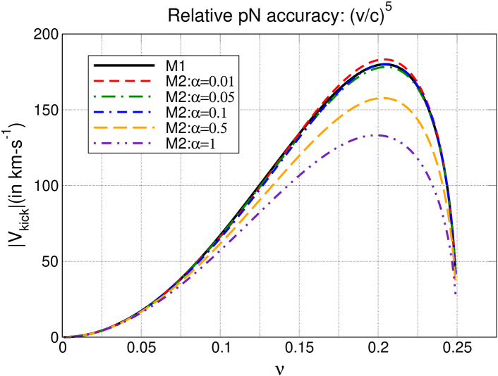
Figure 1: Recoil velocity as a function of the mass parameter $\nu$ (symmetric mass ratio) has been shown. Plot shows a comparison between the results obtained using the two methods (we call them M1 and M2), discussed in Sec.V, that have been used to match the circular orbit at the ISCO to a suitable plunge orbit. It is evident from the figure that the two methods are consistent with each other for smaller values of the parameter $\alpha$.

Equation (29) gives the 2.5PN formula for computing the loss rate of linear momentum in the far-zone of a nonspinning inspiralling compact binary in a quasicircular orbit. In Sec.V, we show how one can numerically estimate the recoil velocity accumulated during the plunge phase, after making some simplifying assumptions. The recoil velocity at the end of the inspiral phase, i.e. at the fiducial ISCO, is given by Eq. (V) whereas the recoil velocity accumulated during the plunge phase is given by Eq. (43). The integral of Eq. (43) needs to be evaluated numerically keeping in mind that appropriate choices for energy and angular momentum at the onset of the plunge phase has been made in order to match the inspiral and plunge orbits at the fiducial ISCO. Figure 1 shows our numerical estimates for the recoil velocity, based on the two methods (we call them M1 and M2) for matching the circular orbit at the fiducial ISCO to a suitable plunge orbit, discussed in the previous section. Figure 1 also shows a comparison between the recoil velocity estimates using the two methods, M1 and M2. It is evident from the figure that results from both the methods are consistent with each other for smaller value of the parameter $\alpha$, defined above. In the case of M2, we have shown curves corresponding to $\alpha=\{0.01,0.05,0.1,0.5,1.0\}$, and one can see that the curves with $\alpha=0.01\,,0.05,{\rm and}\,0.1$ are very close to the curve corresponding to the M1. We also observe that the recoil velocity, for a binary system with $\nu=0.2$, as shown in Fig. 1, is $\sim$179.5 $\rm{km\,s^{-1}}$. This is lower than the 2PN accurate BQW estimate of about 243 $\rm{km\,s^{-1}}$ for the binary with the same mass ratio ($\nu=0.2$). This behavior is due to the presence of large negative coefficients at the 2.5PN order (see Eq. (IV)) which bring down the estimates significantly. Such a behavior is not new to PN calculations, e.g. a similar behavior was observed in Wiseman (1992) at 1PN order (see Fig.1 of Blanchet et al. (2005)), where the use of 1PN accurate results give a lower estimate for the recoil velocity as compared to the one obtained using the Newtonian formulas since the 1PN term again contributes negatively to the recoil velocity.

Note that the estimates presented in Fig. 1 use only the leading order radiation reaction effects for setting initial energy (in M1) and energy and angular momentum (in M2). We repeat the exercise using 2.5PN expressions for relevant quantities beyond the leading order effect and find that changes in estimates are negligible (relative $\%$ changes are less than 0.5$\%$).

As discussed earlier, normally the PN approximations are expected to become less and less reliable beyond the ISCO. This leads to a crude estimate of the accumulated recoil velocity during the plunge phase. Hence, it becomes important to compare our results to some other numerical/analytical estimates, in order to be sure that these estimates are indeed reliable. In the case of the present work the closest comparison for the recoil velocity estimates can be made by comparing our results with those of BQW Blanchet et al. (2005). For a binary with $\nu=0.22$ and $\nu=0.23$, BQW suggest that the recoil velocity should lie in a range, (171-251) $\rm{km\,s^{-1}}$ and (146-220) $\rm{km\,s^{-1}}$, respectively. The uncertainty in their results has been estimated by flexing the 2PN expressions by addition of 2.5PN, 3PN and 3.5PN terms and then computing the maximum variation in their results (see Blanchet et al. (2005) for details). Our estimates of the recoil velocity for a binary with $\nu=0.22$ and $\nu=0.23$ are $172\,\rm{km\,s^{-1}}$ and $155\,\rm{km\,s^{-1}}$, respectively, and thus our estimates lie in the window for the recoil velocity provided by BQW. However, we should note here that our estimates can also change if we add contributions coming from the 3PN and the 3.5PN terms (although changes may be relatively smaller). Currently, such an extension is not possible as we do not have sufficiently accurate inputs in order to perform such computations and thus it will be the subject matter of a work in the future. Our estimates are also consistent with an earlier numerical work Campanelli (2005) which suggests a range of values for recoil velocity between $(100-380)\,\rm{km\,s^{-1}}$ and $(90-290)\,\rm{km\,s^{-1}}$ for $\nu=0.22$ and $\nu=0.23$, respectively. As discussed in Sec. I, Ref. Sopuerta et al. (2007) suggests that maximum recoil velocity estimate for a binary with $\nu=0.2$ in quasicircular orbit lie in a range between (79-216) $\rm{km\,s^{-1}}$. As mentioned above, our estimate for such system is $\sim$179.5 $\rm{km\,s^{-1}}$ and thus is consistent with their estimates.

We witnessed above that inclusion of 2.5PN contributions significantly changed earlier PN estimates for the recoil velocity indicating that contributions at higher orders need to be explicitly assessed due to the asymptotic nature of the PN expansion. As mentioned above, contributions at other high PN orders such as at 3PN and 3.5PN should be included in some future work in order to have better estimates for the recoil velocity, although the changes may be relatively smaller as compared to those brought in by 2.5PN contributions. A numerical study Baker et al. (2006) suggests that the recoil velocity estimates at the fiducial ISCO should be of the order of $\sim$ 14 $\rm{km\,s^{-1}}$ for a binary with $\nu=0.24$ and this estimate matches well with BQW estimates for the same system. This is a relatively higher estimate as compared to our estimate of 2.8 $\rm{km\,s^{-1}}$ at the fiducial ISCO for a system with the same mass ratio. In such a case, we should expect that inclusion of higher order contributions at the 3PN order will contribute to the recoil velocity positively (in contrast to the negative contributions from 2.5PN terms) and thus could bring up the estimates to match with estimates of Baker et al. (2006) and BQW. In addition to this, as a follow-up of this work, one can try to include contributions due to the final ringdown phase using 2.5PN accurate initial conditions and then combine this with the recoil velocity estimates for the inspiral and plunge phase presented here. This will allow one to make more direct comparisons with the results obtained using numerical relativity and the effective one-body approach which include contributions from all three phases of the binary evolution.