RG flows, cycles, and c-theorem folklore

Abstract

Monotonic renormalization group flows of the “c” and “a” functions are often cited as reasons why cyclic or chaotic coupling trajectories cannot occur.  It is argued here, based on simple examples, that this is not necessarily true.  Simultaneous monotonic and cyclic flows can be compatible if the flow-function is multi-valued in the couplings.

year number number identifier LABEL:FirstPage1 LABEL:LastPage#1

Exact general results for renormalization group (RG) flows are important as they may provide physical insight for strongly coupled systems.  The c-theorem for 2D systems Zamolodchikov and the a-theorem for 4D systems Cardy ; Anselmi et al. are two such results that have been established for very broad classes of models Schwimmer .

The c-theorem shows the existence of a monotonically decreasing function of the length scale, $c\left(L\right)$, which interpolates between 2D Virasoro central charges of theories at conformal fixed points, and thereby provides an intuitively correct count of system degrees of freedom — fewer in the infrared than in the ultraviolet.  The a-theorem establishes similar monotonic flow for the induced coefficient of the Euler density, $a\left(L\right)$, for a 4D theory in a curved spacetime background.

It is a common conclusion — a “folk theorem” — based on these monotonically evolving “observables” that the underlying couplings can not have RG trajectories which are limit cycles or undergo more exotic (e.g. chaotic) oscillations (e.g. see 2nd bullet item under §6 in Cardy2010 ).  The point of this note is to explain and illustrate with just one coupling, as simply as possible, why this conclusion is unwarranted.  (Somewhat similar criticism of the monotonic folklore has been proffered in other contexts, involving degenerate Morse function counterexamples for models with vorticity in the flow of several couplings Niemi .)

In principle, we believe cyclic or perhaps even chaotic coupling trajectories are not ruled out by either the $c$- or $a$-theorems, nor are they necessarily excluded by other monotonic “potential flow-functions.”  To illustrate our reasoning, we begin with a very simple example based on a mechanical analogy.  While this example does indeed exhibit both monotonic flow and a cycling trajectory, it has the peculiar feature — insofar as intuitively counting degrees of freedom is concerned — that the monotonic flow is unbounded both above and below.  Nevertheless, we recall there is a field theory model that produces just such behavior LeClair .  We then exhibit another example where the monotonic flow is bounded below and the coupling trajectory is not only cyclic but, in fact, chaotic.

The essential ideas, expressed for a single coupling $x\left(t\right)$, where $t=\ln L$, are given by general statements for a locally gradient RG flow,

$$\frac{dx\left(t\right)}{dt} =\beta\left(x\left(t\right)\right)=-\frac{dC\left(x\left(t\right)\right)}{dx\left(t\right)},$$ (1)

$$\frac{dC\left(x\left(t\right)\right)}{dt} =\frac{dx}{dt}\frac{dC}{dx}=\beta~{}\frac{dC}{dx}=-\left(\frac{dC}{dx}\right)^{2},$$ (2)

and by a specific example of a flow-function, namely,

$$C_{0}\left(x\right)=-\frac{\pi}{4}-\frac{1}{2}\arcsin\left(x\right)-\frac{1}{2}~{}x\sqrt{1-x^{2}}.$$ (3)

The corresponding $\beta$ function is

$$\beta_{0}\left(x\right)=-\frac{d}{dx}~{}C_{0}\left(x\right)=\sqrt{1-x^{2}}.$$ (4)

The RG flow is given by

$$\frac{dx}{dt}=\sqrt{1-x^{2}},$$ (5)

which is easily recognized as a “right-moving” simple harmonic oscillator (SHO) started from rest at $x=-1$.  This of course has a turning point, $x=+1$, reached in finite $\Delta t$, at which point the only way to continue the evolution is to change branches of the square root, $\sqrt{1-x^{2}}\rightarrow-\sqrt{1-x^{2}}$, to produce a “left-moving” SHO.  When this procedure is repeated as turning points are encountered, the cyclic evolution emerges.

In addition, when the first turning point is encountered $C$ switches to a second branch, given by

$$C_{1}\left(x\right)=-\frac{3\pi}{4}+\frac{1}{2}\arcsin\left(x\right)+\frac{1}{2}~{}x\sqrt{1-x^{2}}.$$ (6)

This gives the expected switch between branches for the $\beta$ function,

$$\frac{dx}{dt}=-\frac{d}{dx}~{}C_{1}\left(x\right)=-\sqrt{1-x^{2}}\text{.}$$ (7)

More importantly, this $C$ function continues to decrease monotonically as a function of $t$ after switching branches.

This is easily understood for this simple example just because the monotonically changing $C$ is nothing but the negative of the definite integral of “the oscillator’s kinetic energy” $T=\left(dx/dt\right)^{2}$,

$$C=-\int\beta dx=-\int_{x\left(0\right)=-1}^{x\left(t\right)}\frac{dx}{dt}dx=-\int_{0}^{t}Tdt,$$ (8)

where the integral is taken along the actual trajectory of the oscillator — a path that conserves total “energy,” cf. RG invariants.  (That is to say, $C$ is just the reduced or abbreviated action of Euler, Maupertuis, and Lagrange, or perhaps more consistently with the notation, it is the characteristic function of Hamilton.)

In fact, to obtain the correct evolution for the continuous flow in question, it is absolutely necessary not only to switch between the two branches for $\beta\left(x\right)=\pm\sqrt{1-x^{2}}$, but also to switch among an infinite set of branches for the $C$-function, as successive turning points are encountered.  Thus, as an analytic function, $C$ involves a nontrivial Riemann sheet structure Meurice .  With initial flow to the right, $\left.dx/dt\right|_{t=0}>0$, after $N$ encounters with turning points, the evolution is given by

$$\frac{dx}{dt} =\left(-\right)^{N}\sqrt{1-x^{2}}=-\frac{d}{dx}C_{N}\left(x\right),$$ (9)

$$C_{N}\left(x\right) =-\frac{\pi}{4}\left(1+2N\right)$$

$$-\left(-1\right)^{N}\left(\frac{1}{2}\arcsin\left(x\right)+\frac{1}{2}~{}x\sqrt{1-x^{2}}\right),$$ (10)

where $\arcsin$ is the principal branch of the inverse sine function.  We plot a few branches of $C$ in Figure 1.

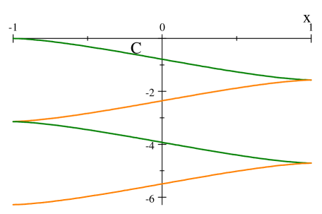
Figure 1: Four branches of the SHO $C\left(x\right)$ function.

More directly, as a function of $t$,

$$C\left(t\right)=-\frac{1}{2}\left(t-\cos t\sin t\right),$$ (11)

which is indeed monotonic in $t$, as shown in Figure 2.

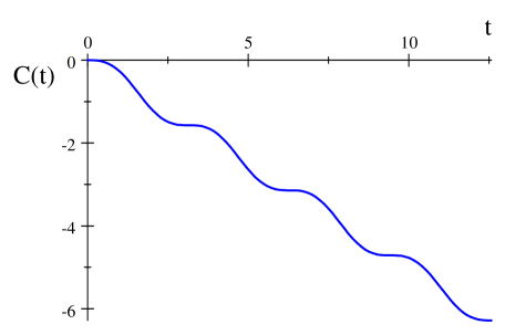
Figure 2: Monotonic flow for the SHO $C\left(t\right)$.

The SHO example of simultaneous monotonic and cyclic flows, while certainly familiar, is perhaps disconcerting, not just because of the multi-valuedness of $C\left(x\right)$, but also because $C\left(t\right)$ is unbounded both above and below.  However, this same cyclic flow may also be observed by selecting different coordinates for the coupling, without changing the physics of the system.  Indeed, the “Russian doll superconductivity model” of Leclair et al. LeClair ; Braaten provides a single flowing coupling $u$ that illustrates what we have in mind.  For that model the RG $\beta$ and corresponding $C$ function are given by innocuous polynomials,

$$\frac{du}{dt}=\frac{1}{2}\left(1+u^{2}\right)\ ,\ \ \ \mathcal{C}=-\frac{1}{2}~{}u\left(1+\frac{1}{3}u^{2}\right).$$ (12)

Despite this uncomplicated local behavior, the global trajectories go through infinite excursions in the course of their cyclic evolution:

$$u\left(t\right)=\tan\left(\frac{1}{2}~{}t+\arctan u\left(0\right)\right).$$ (13)

Thus it is difficult to keep track of the monotonicity of $\mathcal{C}$, if any, as it executes an infinite jump during the course of each cycle.

The system is perhaps easier to grasp upon being expressed in terms of a “dual” coupling, $x$,

$$u=\pm\sqrt{\frac{1+x}{1-x}}\ ,\ \ \ \frac{dx}{dt}=\pm\sqrt{1-x^{2}}.$$ (14)

That is to say, the RG flow of the model is equivalent to the SHO as described earlier.  Note the cyclic switching between the branches of $u\left(x\right)$ corresponding to right-moving (green) and left-moving (orange) SHO motion, including an infinite jump upon reaching $x=1$, as shown in Figure 3.

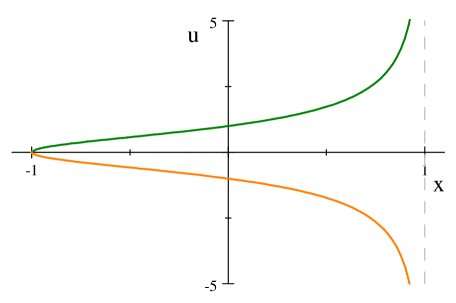
Figure 3: The Russian doll – SHO RG duality.

Similar analysis can be carried out for theories with several coupling constants.  (For models with limit cycles in $4-\varepsilon$ dimensions, see Grinstein ; Nakayama .)  We leave the study of these for another venue.

To complete this brief discussion, we consider a model with a cyclic but chaotic trajectory which also exhibits a monotonic flow-function.  Again, a solvable example involving a single coupling is sufficient to make the point.

Perhaps the simplest system with chaotic RG evolution is the Ising model with imaginary magnetic field, described by the special case of the logistic map with parameter $4$ Dolan ; CZ .  The exact trajectory and $\beta$ function are given by

$$x\left(t\right) =\left(\sin\left(2^{-t}\arcsin\sqrt{x}\right)\right)^{2}\ ,$$ (15)

$$\frac{dx\left(t\right)}{dt} =-\left(\ln 4\right)\sqrt{x\left(t\right)\left(1-x\left(t\right)\right)}\arcsin\sqrt{x\left(t\right)}\ ,$$ (16)

where the $\arcsin$ function in this last expression switches branches upon encountering turning points.  Similarly, the corresponding $C$ function, considered as a function of $x\left(t\right)$, also changes branches at turning points.

The direction of the flow in $t$ is such that the origin is an attractive fixed point in the infrared, so $x\rightarrow 0$ as $L$ & $t=\ln L\rightarrow+\infty$.  On the other hand, $x$ becomes chaotic, exhibiting cycles of arbitrary length, as $L\rightarrow 0$ and $t\rightarrow-\infty$.  That is to say, for any initial $x\in\left(0,1\right]$ the flow for $t>0$ is monotonically toward the fixed point at $x=0$, while for $t<0$ the flow is toward a turning point at $x=1$, where $dx/dt$ reverses and the flow is toward a second turning point at $x=0$ — the zero of $\beta$ at $x=0$ is a fixed point only for the first branch of $\beta$.  As the evolution continues into the UV, with $t<0$, the trajectory oscillates between the pair of turning points, $x=0$ and $x=1$, with increasing average “speed.”

There are an infinite number of branches for both $\beta\left(x\right)$ and $C\left(x\right)$ in this case.  Those branches are given by

$$\beta_{N}\left(x\right)=-\left(\ln 4\right)\sqrt{x\left(1-x\right)}\left\{\left(-\right)^{N}\left\lfloor\tfrac{1+N}{2}\right\rfloor\pi+\arcsin\sqrt{x}\right\},$$

$$C_{N}\left(x\right)=\frac{1}{8}\left(\ln 4\right)\left\{{}\right.4x^{2}\left(x-1\right)^{2}$$ (17)

$$+\left(\sqrt{x\left(1-x\right)}\left(1-2x\right)-\left(-\right)^{N}\left\lfloor\tfrac{1+N}{2}\right\rfloor\pi-\arcsin\sqrt{x}\right)^{2}\left.{}\right\}.$$

Here $\arcsin$ is understood to be the principal branch, $\left\lfloor\cdots\right\rfloor$ is the floor function, and $N$ counts the number of encounters with the trajectory turning points at $x=1$ and $x=0$.  The first three branches of $C\left(x\right)$ are shown in Figure 4.

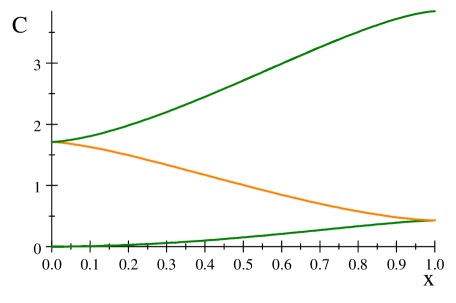
Figure 4: Three branches of the logistic $C\left(x\right)$ function.

As $t\rightarrow\infty$, the flow is toward the origin, with $x\left(+\infty\right)=0$ and $C\left(+\infty\right)=0$, while as $t\rightarrow-\infty$, $C\rightarrow+\infty$.  This is more clearly seen by plotting

$$C\left(t\right)=-\int_{0}^{x\left(t\right)}\beta\left(x\right)dx=\int_{t}^{\infty}\left(\beta\left(x\left(t\right)\right)\right)^{2}dt\ ,$$ (18)

for $0<\left.x\left(t\right)\right|_{t=0}<1$.  The flow of $C$ is monotonic in $t$ and bounded below, $C\geq 0$.  This is shown in Figure 5 for $\left.x\left(t\right)\right|_{t=0}=1/2$.

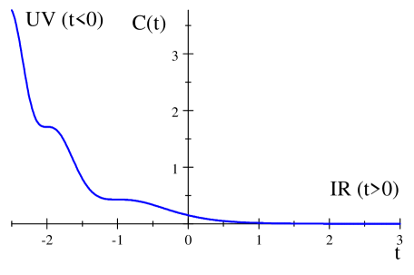
Figure 5: Monotonic flow for the logistic $C\left(t\right)$.

A full discussion of Lagrangian models that realize this second example will have to be given elsewhere.  Suffice it to say here that chaotic RG trajectories have indeed appeared in spin-glass systems McKay ; Bray .  The point we wish to emphasize is that such behavior is not necessarily inconsistent with $c$- and $a$-theorems.

In conclusion, we have argued against the folklore that cyclic RG trajectories are always incompatible with a monotonic potential flow-function producing a gradient flow.  We have shown by examples that monotonic evolution of $C\left(t\right)$ can be consistent with cyclic coupling trajectories given by gradient flows, when the flow-function $C$ is multi-valued in the couplings.

Acknowledgments  We thank D Z Freedman, Ian Low, and Y Meurice for helpful discussions and critical remarks.  This work was supported in part by NSF Award 0855386, and in part by the U.S. Department of Energy, Division of High Energy Physics, under contract DE-AC02-06CH11357.

References

- (1) A B Zamolodchikov, “‘Irreversibility’ of the Flux of the Renormalization Group in a 2D Field Theory” JETP Lett. 43 (1986) 730-732. http://www.jetpletters.ac.ru/ps/1413/article_21504.pdf
- (2) J L Cardy, “Is There a c-Theorem in Four Dimensions?” Phys. Lett. B215 (1988) 749. http://www.sciencedirect.com/science/article/pii/ 0370269388900548
- (3) D Anselmi, D Z Freedman, M T Grisaru, and A A Johansen, “Nonperturbative formulas for central functions of supersymmetric gauge theories” Nucl. Phys. B526 (1998) 543-571. arXiv:hep-th/9708042
- (4) Z Komargodski and A Schwimmer “On Renormalization Group Flows in Four Dimensions” arXiv:1107.3987 [hep-th]
- (5) J Cardy, “The Ubiquitous ‘c’: from the Stefan-Boltzmann Law to Quantum Information” J. Stat. Mech. 1010 (2010) P10004. arXiv:1008.2331 [cond-mat.stat-mech]
- (6) A Morozov and A J Niemi, “Can Renormalization Group Flow End in a Big Mess?” Nucl. Phys. B666 (2003) 311-336. arXiv:hep-th/0304178
- (7) The Riemann sheet structure of various complex coupling flows have been previously discussed in the literature. For example, see A Denbleyker, D Du, Y Liu, Y Meurice, and H Zou, “Fisher’s Zeros as the Boundary of Renormalization Group Flows in Complex Coupling Spaces” Phys. Rev. Lett. 104 (2010) 251601 arXiv:1005.1993 [hep-lat]; Y Meurice and H Zou, “Complex renormalization group flows for 2D nonlinear O(N) sigma models” Phys. Rev. D 83 (2011) 056009 arXiv:1101.1319v3 [hep-lat].
- (8) A LeClair, J M Roman, and G Sierra, “Log-periodic behavior of finite size effects in field theories with RG limit cycles” Nucl. Phys. B700 (2004) 407-435. arXiv:hep-th/0312141
- (9) The Russian doll model of LeClair et al. and other interesting examples of limit cycles are discussed in E Braaten and H-W Hammer, “Universality in Few-body Systems with Large Scattering Length” Phys. Rept. 428 (2006) 259-390 arXiv:cond-mat/0410417 [cond-mat.other]. However, the c-theorem is not discussed therein.
- (10) J-F Fortin, B Grinstein, and A Stergiou “Scale without Conformal Invariance: An Example” Phys. Lett. B704:74-80 (2011). arXiv:1106.2540 [hep-th]
- (11) Y Nakayama “On -conjecture in a-theorem” arXiv:1110.2586 [hep-th]
- (12) B P Dolan, “Chaotic behavior of renormalization flow in a complex magnetic field” Phys. Rev. E52 (1995) 4512-4515. http://pre.aps.org/abstract/PRE/v52/i4/p4512_1
- (13) T L Curtright and C K Zachos, “Renormalization Group Functional Equations” Phys. Rev. D83 (2011) 065019. arXiv:1010.5174 [hep-th]
- (14) S R McKay, A N Berker, and S Kirkpatrick, “Spin-Glass Behavior in Frustrated Ising Models with Chaotic Renormalization-Group Trajectories” Phys. Rev. Lett. 48 (1982) 767–770. http://prl.aps.org/abstract/PRL/v48/i11/p767_1
- (15) A J Bray and M A Moore, “Chaotic Nature of the Spin-Glass Phase” Phys. Rev. Lett. 58 (1987) 57–60. http://prl.aps.org/abstract/PRL/v58/i1/p57_1