Photonic Passbands and Zeropoints for the Strömgren $uvby$ System.

Abstract

Photonic passbands have been derived for the $uvby$ standard system by convolving the original filter passbands of Strömgren and Perry with atmospheric extinction and the QE of a cooled 1P21 photomultiplier tube. Using these new passbands, synthetic photometry was calculated for all the stars in the extensive NGSL and MILES spectrophotometric libraries and compared with the homogenised $b-y$, $m_{1}$ and $c_{1}$ indices in the Hauck-Mermilliod 1998 catalog and the derived $u-v$ and $v-b$ colors. Excellent agreement between observed and synthetic photometry was achieved with regression slopes near unity. Slightly better fits were obtained by considering stars with $b-y<$ 0.5 and $b-y>$ 0.5, separately. It is recommended that these new passbands be used together with the provided transformation equations to generate synthetic photometry from model atmosphere fluxes and observed spectrophotometry. Synthetic photometry was also carried out using the natural system of the 4-channel spectrograph-photometers and those of Cousins and Eggen in order to explore the systematic differences that could be expected between their instrumental systems and the standard system.

1 Introduction

The Strömgren $uvby$ system (Strömgren, 1966), is a widely used intermediate-band photometric system comprising data for more than 63,300 stars in the homogenised Hauck & Mermilliod (1998) catalog. It has long been considered a precise and accurate standard system that is very useful for determining temperatures and effective gravities of B, A, F and early- G stars and metallicities of F and G stars. However, the use of different filters at many observatories and the extension of the photometry to late-G and K stars and to supergiants and reddened stars has resulted in significant systematic differences in the instrumental systems between observers. The recommended method of photometric data reduction to derive the indices $c_{1}=(u-v)-(v-b)$ and $m_{1}=(v-b)-(b-y)$, rather than the colors $u-v$, $v-b$ directly, has also resulted in larger uncertainties in the transformed indices, mainly for the cooler stars. These problems have been vividly illustrated and discussed by Manfroid (1984); Manfroid & Sterken (1987).

A large database of excellent $uvby$ photometry has been obtained with the four 4-channel spectrograph-photometers (Helt et al., 1987) on telescopes at Kitt Peak, La Silla and San Pedro Martir (eg. Olsen, 1983, 1993; Schuster & Nissen, 1988). Fig 1 in Olsen (1983) shows the complicated decision processes carried out to transform this well defined and stable natural system photometry onto the standard system. Cousins (1987) also discussed the non-linearities involved in successively transforming his E-region photometry onto the standard system and Eggen (1976) outlined issues associated with too-narrow a $v$ filter. Given these different and complex transformations one may wonder whether passbands can be defined that accurately represent the homogenised $uvby$ system.

In the last few years, two libraries of accurate higher resolution (R$\sim$1000-2000) spectrophotometric data have become available - NGSL (Heap & Lindler, 2007, http://archive.stsci.edu/prepds/stisngsl/index.html) and MILES (Sanchez-Blazquez et al., 2006, http://www.iac.es/proyecto/miles/) and most of the stars in these spectral libraries also have Hipparcos $H_{p}$ magnitudes - enabling Bessell & Murphy (2011) to renormalize the spectrophotometry on to a precise absolute scale by synthesizing the $H_{p}$ magnitudes. Many of these stars are also in the Hauck & Mermilliod (1998) $uvby$ catalog thus providing the opportunity to critically compare the synthetic $uvby$ photometry with the standard values.

2 The $uvby$ passbands

Matsushima (1969) and Crawford & Barnes (1979) published transmissions of the KPNO $uvby$ filter set No.1 that was used when setting up the original $uvby$ system by Strömgren & Perry (1965). These filter functions are considered to be the best starting point for synthetic $uvby$ photometry calculations. Synthetic photometry based on model atmosphere fluxes have been computed by many authors (Matsushima, 1969; Relyea & Kurucz, 1978; Kurucz, 1979; Clem et al., 2004; Önehag et al., 2009) and while most have convolved the filter functions with a 1P21 sensitivity function, Al mirror reflectivity and 1 airmass of extinction, some (eg Matsushima, 1969; Maiz Appellaniz, 2006) have used the filter transmissions directly.

The product of the filter passband, the atmospheric transmission, the mirror reflectivity and the detector sensitivity function is called the system response function or system passband. In the past, the detector sensitivity function that was used related to the energy measured. Nowadays with photon counting detectors being the norm, the detector sensitivity function used relates to the number of photons measured. The resultant system response functions or system passbands therefore differ depending whether they reflect the energy of the photons or the number of photons. As modern synthetic photometry packages, such as $\it{synphot}$ assume that system response functions are in the photon form, we will use that form in this paper and also use the terms photonic response function or photonic passband to distinguish them from the alternative energy forms.

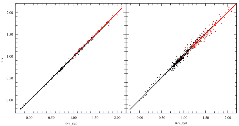
Figure 6: The $u-v$ regressions.

The 1P21 sensitivity function is from Kurucz (1979, table 7); this has the same UV-cuton as measured by Bessell (1979, table1.1) and appears to have a similar red cutoff to that measured by Young (1963, fig 6). It is presumed to be in terms of the photocathode radiant response (in units of mA W^-1) and we have converted it into QE to derive the photonic responses (see Bessell & Murphy, 2011). The mirror reflectivity (see values in Helt et al., 1987) was neglected, but we applied 1.2 air masses of typical Siding Spring Observatory (1200m) extinction.

In Table 1 we list our adopted normalized system photonic passbands $S_{x}(\lambda)$ for $u$, $v$, $b$ and $y$, and in Fig 1 we show the passbands compared to those of Maiz Appellaniz (2006) and the 4-channel spectrograph-photometers (Helt et al., 1987) (see below).

3 Comparison between synthetic photometry and standard photometric values

The synthetic photometry was computed by evaluating, for each of the $uvby$ bands, the expression (see Bessell & Murphy, 2011)

mag_x = AB_ν $-$ ZP_x

(1)

where

AB = $-2.5\log\frac{\displaystyle\int{f_{\nu}(\nu)S_{x}(\nu)d\nu/\nu}}{\displaystyle\int{S_{x}(\nu)d\nu/\nu}}-48.60$ = $-2.5\log\frac{\displaystyle\int{f_{\lambda}(\lambda)S_{x}(\lambda)\lambda d\lambda}}{\displaystyle\int{S_{x}(\lambda)c\,d\lambda/{\lambda}}}-48.60$

(2)

and $f_{\nu}(\nu)$ is the observed absolute flux in erg cm^-2 sec^-1 Hz^-1, $f_{\lambda}(\lambda)$ is the observed absolute flux in erg cm^-2 sec^-1 Å^-1, $S_{x}(\lambda)$, is the photonic passband (Table 1), $\lambda$ is the wavelength in Å, and ZP_x is the zeropoint magnitude for each band.

For accurate synthetic photometry it is important that the passbands provided to the integration routines are well sampled and smooth. It is necessary therefore, to interpolate the coarsely sampled values of the passbands in Table 1 to a finer spacing of a few Å using a univariate spline or a parabolic interpolation routine.

Firstly, the CALSPEC stis005 spectrum for Vega was used to derive the AB_ν mag zeropoints of $-$0.308, $-$0.327, $-$0.187 and $-$0.027 for $u$, $v$, $b$ and $y$, respectively, adopting for Vega, $y$=0.03, (Bessell, 1983); $(b-y)$=0.004, $m_{1}$=0.157 and $c_{1}$=1.088, (Hauck & Mermilliod, 1998).

We then computed synthetic colors for all the renormalized NGSL (376) and MILES (830) spectra (Bessell & Murphy, 2011) and matched the stars against the homogenised Hauck & Mermilliod (1998) catalog, yielding 259 and 535 objects, respectively, with both spectrophotometry and $uvby$ photometry.

The color differences and index differences were regressed against $b-y$, $m_{1}$ and $c_{1}$, and little evidence of residuals that were a continuous function of color were found. Any variation with color that was evident was better dealt with by splitting the sample into blue and red stars, rather than fitting an overall color term. Those stars with $b-y>$ 0.5 also showed slightly more scatter than did the bluer stars which could have been anticipated since the $uvby$ system was initially standardized for the bluer stars and extended later to the redder stars using a greater range of instrumental systems and only a few red standards. (The higher scatter in the MILES comparison for those measures involving the $u$ band in this paper should be discounted because we extrapolated their UV fluxes somewhat crudely using model atmosphere fits to the rest of the spectrum.) Overall, it was extremely gratifying to see the near unity slopes and small scatter in the comparisons, indicating that the realised passbands are an excellent representation of the standard system.

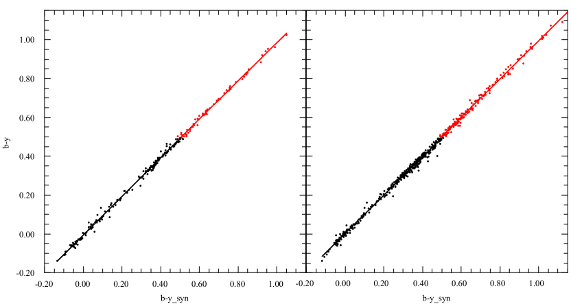
Figure 2: The $b-y$ regressions. Stars with $b-y<$ 0.5 (black), $b-y>$ 0.5 (red). NGSL stars left; MILES stars right. The coefficients of the linear fits are given in Table 2.

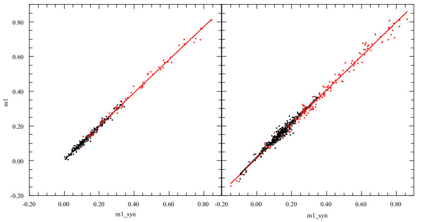
Figure 3: The $m_{1}$ regressions.

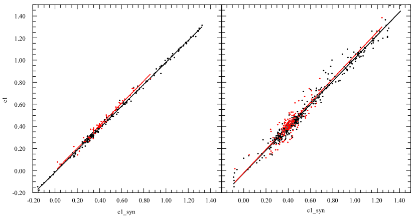
Figure 4: The $c_{1}$ regressions.

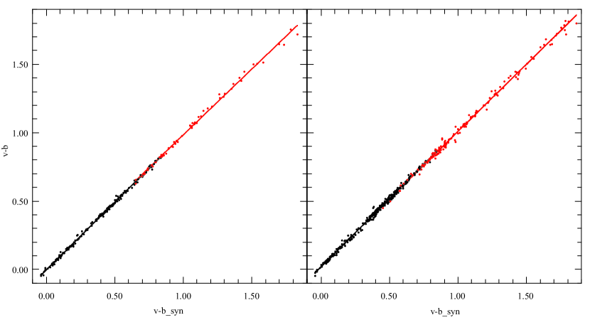
Figure 5: The $v-b$ regressions.

Figures 2 - 6 show the regressions for $b-y$, $m_{1}$, $c_{1}$, $u-v$ and $v-b$ overlayed with the lines fitted to the blue and red spectra separately. There were about 185 blue and 70 red spectra in the NGSL sample, and 360 blue and 150 red spectra in the MILES sample. In many cases the same fitted line for blue and red stars could suffice within the uncertainties, but for some colors and indices, small blue/red star differences were evident.

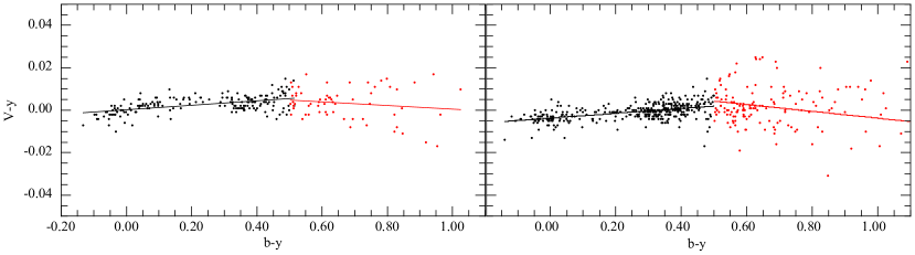
Figure 7: The synthetic $V-y$ regressions.

Figure 7 shows the synthetic $V-y$ regressions against $b-y$; the $V$ passband is from Bessell & Murphy (2011). The mean wavelength of the $y$ band is clearly very close to that of the $V$ band.

In Table 2 are listed the results of the least-square linear fits to the regressions, including the uncertainties in the coefficients and the residual rms. It is recommended that the transformation equations determined from the space-based NGSL spectra be used to convert synthetic photometry onto the same system as the Hauck & Mermilliod (1998) catalog; however, the equations from the MILES fits are in excellent agreement with those from the NGSL spectra, although the scatter is slightly higher. It should also be noted that the slopes of the transformations are of the same order as the observational values reported by Crawford & Barnes (1979) using KPNO filter set No 1.

4 Review of some other natural $uvby$ systems

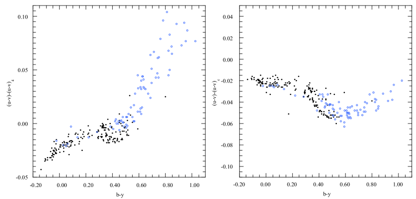
Figure 8: The synthetic $\Delta$ ($u-v$) regressions for the natural 4-channel system (Helt et al., 1987) (left) and Cousins (1987) (right). Dwarfs (black dots), giants (blue open circles)

Manfroid (1984) was the first to use synthetic photometry to explore the systematic effects that different instrumental system passbands have on $uvby$ photometry. This was further discussed by Manfroid & Sterken (1987). We decided to use the NGSL spectrophotometric data to examine two widely used natural $uvby$ systems, the 4-channel spectrograph-photometers (Helt et al., 1987) and that of Cousins (1987), in order to explore the systematic differences that could be expected between their instrumental systems and that presented in this paper as representing the standard system. The photonic passband of Helt et al. (1987) are plotted in Fig 1 and listed in Table 3 (the narrow spike in the published Helt et al. $u$ passband has been smoothed over). In Fig 8 and 9 we show the computed differences in the $u-v$ and $v-b$ colors plotted against $b-y$ for the NGSL spectra. The division between dwarfs and giants in these plots was made at log g $=3.5$; higher gravity stars are plotted as dwarfs and lower gravity as giants. The total range of the vertical scales of the two plots in each figure is the same.

The differences shown in the plots are very similar to those indicated by Olsen (1983), Cousins (1987), Manfroid (1984) and Manfroid & Sterken (1987). It is interesting to see the dwarf-giant separation for the cooler stars and the increase in scatter for the cooler giants.

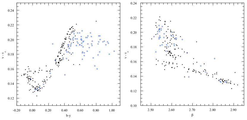
Figure 10: Synthetic $\Delta$ $v$ versus (b-y) and $\beta$ for the narrow $v$ filter. Dwarfs (black dots), giants (blue open circles)

The effect of the narrow $v$ band ($\sim$110Å fwhm) reported by Eggen (1976) was also investigated. An Eggen-type $v$ band was constructed by simply scaling the half-width of the standard band and keeping the same central wavelength. In Fig 10 are shown the computed difference in the measured $v$ magnitude plotted against $b-y$ and $\beta$. Large difference are seen for the hotter stars due to the strength of the H$\delta$ line and in the cool giants and dwarfs due mainly to the atomic and molecular features.

As pointed out by Manfroid & Sterken (1987), these comparisons underline the difficulties that observers with non-standard passbands experience in trying to standardize their internally precise $uvby$ photometry.

5 Summary

We have derived passbands for the $uvby$ system using the KPNO No.1 filter transmissions of Matsushima (1969) and Crawford & Barnes (1979) convolved with the cathode sensitivity function of a 1P21 photomultiplier tube, and an extinction of 1.2 airmasses. These were converted to photonic passbands by dividing by the wavelength and then renormalized. They are listed in Table 1 and shown in Figure 1.

Initial AB mag $uvby$ zeropoints were derived from the stis005 spectrum of Vega. Synthetic photometry was then carried out on the extensive NGSL and MILES spectrophotometric catalogs and compared with the observational data in the homogenised Hauck & Mermilliod (1998) catalog. Excellent linear fits with near unity slopes were made to the synthetic-observational regressions showing how well the passbands represent the standard system. The coefficents of the fitted lines are given in Table 2 and the equations from the NGSL stars should be used to produce standard photometric values from synthetic photometry of observed spectrophotometric fluxes or model atmosphere fluxes.

Some non-standard passbands of two well defined natural $uvby$ systems were also synthesized and shown to produce similar systematic differences to those reported by the users. These effects limit the accuracy with which transformations to the standard system can be made, mainly for the cooler stars and the hotter reddened stars. The narrow $v$-band used by Eggen (1976) and others was shown to produce the largest systematic differences and supports Eggen’s decision to not standardize his M1 and C1 photometry.

However, in spite of these limitations, observers have generally been successful in transforming their photometry onto the standard system and Hauck & Mermilliod (1998) have been successful in producing a very useful homogenised $uvby$ catalog. Hopefully, the revised passbands and transformation equations presented here will enable more reliable theoretical calibrations of Strömgren indices to be made using model atmosphere fluxes.

Table 1: Normalized $uvby$ photonic passbands

Wave	$u$	Wave	$v$	Wave	$b$	Wave	$y$
3150	0.000	3750	0.000	4350	0.000	5150	0.000
3175	0.004	3775	0.003	4375	0.010	5175	0.022
3200	0.050	3800	0.006	4400	0.023	5200	0.053
3225	0.122	3825	0.016	4425	0.039	5225	0.082
3250	0.219	3850	0.029	4450	0.056	5250	0.116
3275	0.341	3875	0.044	4475	0.086	5275	0.194
3300	0.479	3900	0.060	4500	0.118	5300	0.274
3325	0.604	3925	0.096	4525	0.188	5325	0.393
3350	0.710	3950	0.157	4550	0.287	5350	0.579
3375	0.809	3975	0.262	4575	0.457	5375	0.782
3400	0.886	4000	0.404	4600	0.681	5400	0.928
3425	0.939	4025	0.605	4625	0.896	5425	0.985
3450	0.976	4050	0.810	4650	0.998	5450	0.999
3475	1.000	4075	0.958	4675	1.000	5475	1.000
3500	0.995	4100	1.000	4700	0.942	5500	0.997
3525	0.981	4125	0.973	4725	0.783	5525	0.938
3550	0.943	4150	0.882	4750	0.558	5550	0.789
3575	0.880	4175	0.755	4775	0.342	5575	0.574
3600	0.782	4200	0.571	4800	0.211	5600	0.388
3625	0.659	4225	0.366	4825	0.130	5625	0.232
3650	0.525	4250	0.224	4850	0.072	5650	0.143
3675	0.370	4275	0.134	4875	0.045	5675	0.090
3700	0.246	4300	0.079	4900	0.027	5700	0.054
3725	0.151	4325	0.053	4925	0.021	5725	0.031
3750	0.071	4350	0.039	4950	0.015	5750	0.016
3775	0.030	4375	0.027	4975	0.011	5775	0.010
3800	0.014	4400	0.014	5000	0.007	5800	0.009
3825	0.000	4425	0.006	5025	0.003	5825	0.004
3850	0.000	4450	0.000	5050	0.000	5850	0.000

Table 2: Zeropoints and slopes in the form I_std = a₀ + a₁I_syn from synthetic photometry

			NGSL					MILES
index	a0	$\pm$	a1	$\pm$	rms	a0	$\pm$	a1	$\pm$	rms
$b-$y	$-$0.007	0.001	0.997	0.005	0.007	0.002	0.001	0.986	0.004	0.010
	0.004	0.007	0.979	0.010	0.007	0.010	0.005	0.985	0.007	0.013
$m_{1}$	0.005	0.002	0.963	0.010	0.022	0.021	0.002	0.988	0.012	0.019
	0.011	0.005	0.951	0.012	0.022	0.015	0.004	0.979	0.010	0.026
$c_{1}$	$-$0.016	0.002	0.994	0.004	0.035	$-$0.025:	0.005	1.041:	0.008	0.052:
	$-$0.003	0.009	1.018	0.021	0.035	$-$0.023;	0.017	1.064:	0.040	0.075:
$v-b$	$-$0.002	0.001	0.987	0.003	0.020	0.019	0.001	1.001	0.003	0.011
	0.024	0.009	0.961	0.008	0.019	0.027	0.006	0.982	0.005	0.022
$u-v$	$-$0.022	0.003	0.995	0.003	0.035	$-$0.001:	0.008	1.018:	0.008	0.045:
	$-$0.008	0.017	0.987	0.012	0.035	0.020:	0.023	0.991:	0.015	0.058:
$V-y$	0.000	0.000	0.011	0.001	0.002	$-$0.004	0.000	0.011	0.001	0.004
	0.009	0.004	$-$0.009	0.007	0.003	0.012	0.004	-0.160	0.006	0.011

Table 3: Normalized (Helt et al., 1987) $uvby$ photonic passbands

Wave	$u$	Wave	$v$	Wave	$b$	Wave	$y$
3320	0.000	4000	0.000	4560	0.000	5340	0.000
3340	0.349	4020	0.427	4580	0.304	5360	0.389
3360	0.492	4040	0.754	4600	0.576	5380	0.672
3380	0.581	4060	0.884	4620	0.906	5400	0.912
3400	0.687	4080	0.979	4640	0.994	5420	1.000
3420	0.789	4100	0.995	4660	1.000	5440	0.982
3440	0.835	4120	1.000	4680	0.969	5460	0.953
3460	0.879	4140	0.996	4700	0.921	5480	0.913
3480	0.926	4160	0.942	4720	0.871	5500	0.850
3500	0.960	4180	0.742	4740	0.864	5520	0.798
3520	0.982	4200	0.440	4760	0.804	5540	0.759
3540	0.992	4220	0.219	4780	0.522	5560	0.725
3560	1.000	4240	0.000	4800	0.186	5580	0.631
3580	0.996			4820	0.000	5600	0.424
3600	0.991					5620	0.213
3620	0.973					5640	0.000
3640	0.934
3660	0.816
3680	0.356
3700	0.000

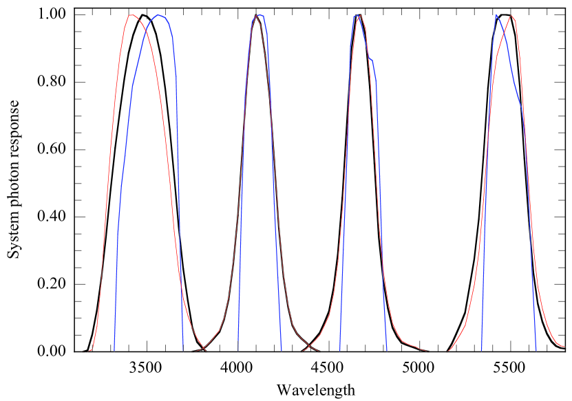
Figure 1: The photonic passbands in this paper (black) compared with those of Maiz Appellaniz (2006)(red) and Helt et al. (1987)(blue).

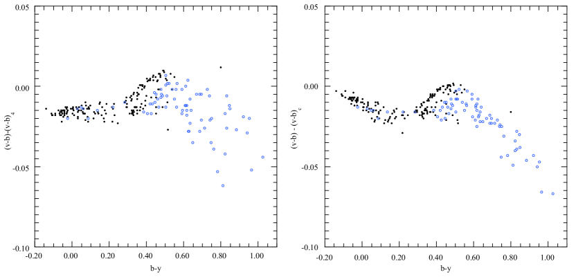
Figure 9: The synthetic $\Delta$ ($v-b$) regressions for the natural 4-channel system (Helt et al., 1987) (left) and Cousins (1987) (right). Dwarfs (black dots), giants (blue open circles)

References

- Bessell (1979) Bessell, M.S., 1979, PASP, 91, 589
- Bessell (1983) Bessell, M.S., 1983, PASP, 95, 480
- Bessell & Murphy (2011) Bessell, M.S. & Murphy, S.J., 2011, PASP, submitted
- Cousins (1987) Cousins, A.W.J., 1987, SAAOCirc, 11, 93
- Clem et al. (2004) Clem, J.L., VandenBerg, D.A., Grundahl, F. & Bell, R.A., 2004, AJ, 127, 1227
- Crawford & Barnes (1979) Crawford, D.L. & Barnes, J.V., 1979, AJ, 75, 978
- Eggen (1976) Eggen, O.J., 1976, PASP, 88,732
- Hauck & Mermilliod (1998) Hauck, B. & Mermilliod, M., 1998, A&AS, 129, 431
- Heap & Lindler (2007) Heap, S.R. & Lindler, D. 2007, IAUS, 241, 95
- Helt et al. (1987) Helt, B.E., Franco, G.A.P. & Florentin Nielsen, R., 1987, ESO Conf., 26, 89
- Kurucz (1979) Kurucz, R.L., APJS, 40, 1
- Maiz Appellaniz (2006) Maiz Apellaniz, J., 2006, AJ, 131, 1184
- Manfroid (1984) Manfroid, J., 1984, A&A, 141, 101
- Manfroid & Sterken (1987) Manfroid, J. & Sterken, C., 1987, A&AS, 71, 539
- Matsushima (1969) Matsushima, S., 1969, APJ, 158, 1137
- Olsen (1983) Olsen, E.H., 1983, A&AS, 54, 55
- Olsen (1993) Olsen, E.H., 1993, A&AS, 102, 89
- Önehag et al. (2009) Önehag, B., Gustafsson, B., Eriksson & Edvardsson, B., 2009, A&A, 498, 527
- Relyea & Kurucz (1978) Relyea, L.J. & Kurucz, R.L., 1978, ApJS, 37, 45
- Sanchez-Blazquez et al. (2006) Sanchez-Blazquez, P., Peletier, R. F., Jimenez-Vicente, J., Cardiel, N., Cenarro, A. J., Falcon-Barroso, J., Gorgas, J., Selam, S. & Vazdekis, A., 2006, MNRAS,371,703
- Schuster & Nissen (1988) Schuster, W.J. & Nissen, P.E., 1988, A&AS, 73, 225
- Strömgren (1966) Strömgren, B., 1966, ARAA, 4, 433
- Strömgren & Perry (1965) Strömgren, B. & Perry, C., 1965, unpublished, privately circulated
- Young (1963) Young, A.T., 1963, ApplOpt, 2, 51