Astrometry and radial velocities of the planet host M dwarf GJ 317: new trigonometric distance, metallicity and upper limit to the mass of GJ 317b

Abstract

We have obtained precision astrometry of the planet hosting M dwarf GJ 317 in the framework of the Carnegie Astrometric Planet Search project. The new astrometric measurements give a distance determination of 15.3 pc, 65% further than previous estimates. The resulting absolute magnitudes suggest it is metal rich and more massive than previously assumed. This result strengthens the correlation between high metallicity and the presence of gas giants around low mass stars. At 15.3 pc, the minimal astrometric amplitude for planet candidate GJ 317b is 0.3 milliarcseconds (edge-on orbit), just below our astrometric sensitivity. However, given the relatively large number of observations and good astrometric precision, a Bayesian Monte Carlo Markov Chain analysis indicates that the mass of planet b has to be smaller than twice the minimum mass with a 99% confidence level, with a most likely value of 2.5 $M_{Jup}$. Additional RV measurements obtained with Keck by the Lick-Carnegie Planet search program confirm the presence of an additional very long period planet candidate, with a period of 20 years or more. Even though such an object will imprint a large astrometric wobble on the star, its curvature is yet not evident in the astrometry. Given high metallicity, and the trend indicating that multiple systems are rich in low mass companions, this system is likely to host additional low mass planets in its habitable zone that can be readily detected with state-of-the-art optical and near infrared RV measurements.

1 Introduction

Astrometric observations complementing radial velocity measurements provide the only means to measure the dynamical masses of long period non-transiting exoplanets. The astrometric technique has been largely unsuccessful in the detection of low mass companions, mainly due to strong systematic effects that are difficult to calibrate through the noise added by the Earth’s atmosphere. An example is the planet candidate around the M8.5V star VB 10 (Pravdo & Shaklan, 2009), which could not be confirmed by radial velocities (Bean et al., 2010; Anglada-Escudé et al., 2010) nor by further astrometric observations (Lazorenko et al., 2011). Compared to other techniques such as precision Doppler measurements, astrometry cannot be corrected using laboratory standards and relies upon measuring the relative motion of the target star with respect to a number of background and (desirably) slow moving distant sources. Typical FGK planet hosting dwarfs that should show the largest astrometric wobbles are too bright to be observed simultaneously with background sources, so the perturbing effect of the atmosphere and time dependent geometric field distortions cannot be easily calibrated in the observations. Some success has been achieved from space. Posterior analysis of HIPPARCOS astrometry has been used to put upper limits on the masses of detected RV companions, ruling out that most of them are low mass stars in face on orbits (Pourbaix & Arenou, 2001). A recent reanalysis by Reffert & Quirrenbach (2011) of the residuals to the new HIPPARCOS solution (van Leeuwen, 2010) has been able to confirm the planetary nature of 9 objects and a number of brown dwarf candidates by putting upper limits to their masses. In the same study, the planetary signal could be recovered on 3 systems. Also, precision astrometry of bright stars has been measured using the Fine Guidance Sensors on board the Hubble Space Telescope (e.g. Martioli et al., 2010; McArthur et al., 2010, for the most recent results). Up to now, these are the only astrometric measurements sensitive enough to place actual constraints on the masses of long period planet candidates and are all obtained by space-based observations.

The Carnegie Astrometric Planet Search is a ground-based program focused on the detection of giant planets around nearby, low mass stars. The astrometric wobble imprinted by a planet on the central star is inversely proportional to the stellar mass (the smaller the mass, the larger the signal). Also, low mass stars (M and L dwarfs) are much fainter than typical F,G and K stars (the most common targets of the RV surveys), simplifying the simultaneous observations of the targets and faint background reference sources. A central part of the project has been the construction of a specialized camera (Boss et al., 2009). CAPSCam uses a Hawaii-2RG HyViSI hybrid array that allows the definition of an arbitrary guide window which can be read out (and reset) rapidly, repeatedly, and independently of the rest of the array. This guide window is centered on our relatively bright target stars, with multiple short exposures avoiding saturation. The rest of the array then integrates for prolonged periods on the background reference grid of fainter stars. This dramatically extends the dynamic range of the composite image. This HyViSI detector is the heart of the CAPSCam concept. A full description of the program, instrument performance and characteristics is given in Boss et al. (2009). The high dynamical range enabled by the guide window mode permits the observation of stars as bright as magnitude I = 9 using integration times as short at 0.2 sec on the target object. Even though the best epoch precision is at the level of 0.4 mas, the long term accuracy is limited by (yet) unknown systematic effects, that are more pronounced on bright objects. The typical epoch-to-epoch precision at the bright end is about 1 mas. As a complementary part of the planet search program, we follow-up a handful of long period RV planet candidates that should produce a detectable astrometric signal (that is, with a semiamplitude above 0.5 mas). GJ 317 is one such star (I $\sim$ 9.32, Rojo & Ruiz, 2003). Johnson et al. (2007) (hereinafter JB07) reported the detection of a $\sim$700 day period planet candidate with a minimum mass of 1.2 $M_{Jup}$ and evidence of an additional companion (GJ 317c) with a period of several thousand days. Using that orbital solution and the previously reported distance ($\sim$9.7 pc, Jenkins, 1963), we estimated a minimum astrometric amplitude (assuming an edge-on orbit) of $\sim$0.58 mas for GJ 317b. With an epoch-to-epoch precision of 1 mas, this is a challenging but doable measurement. Assuming a median inclination of 45 deg, one would expect a semiamplitude of 0.84 mas.

The star has been continuously monitored by the Lick-Carnegie Planet Search group using Keck/HIRES, increasing the number of RV measurements from 18 (JB07) to 38. These additional measurements should better constrain the nature of the long period planet and permit a search for lower amplitude signals. GJ 317 is a nearby star of astrobiological interest. Its low mass and Solar System-like configuration (two outer giant planets) make it an outstanding candidate to search for potentially habitable planets with radial velocity observations.

2 Observations: Astrometry

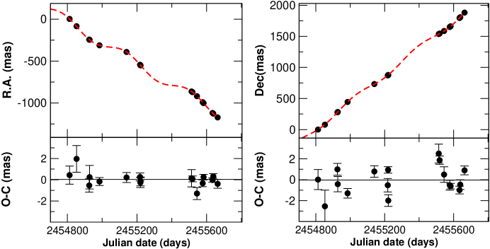
Figure 1: Top panels. Differential astrometry of GJ 317 measured with CAPScam as a function of time. The best fit to the parallax and proper motion is illustrated by the red dashed line. Bottom panels. The residuals after removing the parallax and proper motion.

We have used CAPSCam mounted on the 2.5-m du Pont telescope at Las Campanas Observatory to obtain 18 astrometric observations of GJ 317 with a time baseline of 2.5 years. The observations cover 1.5 orbital periods of GJ 317b. Since the RV measurements constrain 5 out of 7 of the orbital parameters (period $P$, minimum mass $M\sin i$, initial mean anomaly $M_{0}$, eccentricity $e$, and argument of the periastron $\omega$), the astrometric measurements only need to constrain the two remaining elements (argument of the node $\Omega$ and orbital inclination $i$), plus the classic astrometric observables (position, proper motion $\mu_{\alpha}$ and $\mu_{\delta}$; and the parallax $\Pi$, see Appendix A).

A typical observing epoch consists spending one hour of telescope time to obtain 30-50 images on the full $\sim 6\prime\times 6\prime$. The integration time of each image varies between 45 to 60 seconds depending on seeing and environmental conditions. Guide-window exposure time is always set to 0.2 seconds on GJ 317. Therefore, between 225 and 300 guide-window reads are obtained and coadded to each image of the full field. The field around GJ 317 is rich in background reference stars. The astrometric precision (intranight centroid scatter) is computed by comparing the position of the target star to the reference stars in each of the 30-50 images per epoch. The epoch-to-epoch accuracy is estimated by comparing the observations to the best fit astrometric model (see Appendix A). For GJ 317 in particular, the typical intranight precision is of the order of 0.5 mas. This precision is illustrated as the error bars in Figure 1. However, the typical epoch-to-epoch accuracy is 0.6 mas in R.A. and 1.2 mas in declination, indicating that a significant source of uncertainty is not random errors but uncalibrated field distortion effects (systematic errors), especially in Declination. One epoch (January 2009) was rejected because the camera shutter stopped working, causing severe saturation and charge persistence problems on the target star. The relative astrometric measurements used in the analysis are given in Table 1 and illustrated in Figure 1. The residuals (bottom panels) are obtained by subtracting the best fit to the parallax and proper motion. An overview of the astrometric solution and relevant statistical quantities are given in Section 4. Further details on the astrometric data reduction procedure are given in Appendix A.

Table 1: Differential astrometry of GJ 317

Julian date (days)	R.A.	Dec.	Unc. R.A.	Unc. Dec.
(days)	(mas)	(mas)	(mas)	(mas)
2454812.73956	2.53	0.45	0.85	0.96
2454852.70285	-84.44	78.60	1.25	1.54
2454925.62847	-243.32	278.06	0.62	0.56
2454927.64450	-245.94	282.56	1.10	0.73
2454984.47159	-312.21	443.92	0.37	0.45
2455139.85431	-391.52	732.33	0.47	0.54
2455217.72615	-543.92	871.29	0.37	0.64
2455219.71792	-549.13	877.34	0.46	0.30
2455220.72072	-551.37	876.73	0.41	0.55
2455513.86011	-862.40	1538.05	0.81	0.90
2455518.86210	-870.26	1544.93	0.27	0.40
2455544.83951	-919.02	1586.19	0.56	0.74
2455577.73092	-990.53	1650.71	0.32	0.47
2455582.66573	-1001.48	1661.73	0.25	0.26
2455634.52079	-1118.87	1795.91	0.20	0.37
2455638.55749	-1126.62	1807.95	0.24	0.46
2455663.52245	-1171.86	1882.12	0.41	0.42

The measured motion of GJ 317 is relative to the background stars. As discussed in Appendix A, the reference stars are matched to their predicted positions that, in turn, are also refined on each iteration of the astrometric iterative solution. As all the stars have the same parallactic motion (except for the amplitude), the average parallactic motion of the reference frame cannot be derived from relative astrometric observations. This translates into a zero–point ambiguity in the measured distance to the target that needs to be corrected. After the final solution is obtained for all the stars in the field, the measured differential parallax of some of the references is used to estimate the zero–point correction as follows. Using the B, J, H and K magnitudes from the NOMAD catalog (Zacharias et al., 2004), photometric distances are obtained to 7 stars with all these colors available. The information for all the reference stars and is given in Appendix A. Photometric distances to main sequence stars estimated this way can have uncertainties of up to 20% of their actual values. Note, however, that a star at 330 pc will have a parallax of 3 mas and a corresponding uncertainty in the photometric parallax of only 0.6 mas. In comparison, a star at 50 pc would have a parallax of 20 mas and a corresponding uncertainty of 4 mas. Therefore, we only use stars with nominal photometric distances beyond 300 pc to obtain a more secure determination of the zero–point. The average difference between the photometric parallaxes and the measured ones is the desired offset and amounts to 0.23 $\pm$ 0.1 mas for this field in particular. This offset is added to the measured parallax of GJ 317 to provide the final distance determination in Table 2. The fact that the dispersion around the average zero-point is small, indicates that this strategy is robust against uncertainties in the photometry and the models. To prove that our procedure is essentially correct, Figure 2 shows the parallaxes of several CAPS program stars compared to the ones published in the literature. We actually found several outliers (not shown here) that typically correspond to previous parallactic measurements done with a small number of epochs and a formal uncertainties larger than 5 mas. These cases and an overview of the CAPS sample will be discussed in a future publication. For the stars shown here, the measurements coincide within the published uncertainties and we find no systematic zero-point offset.

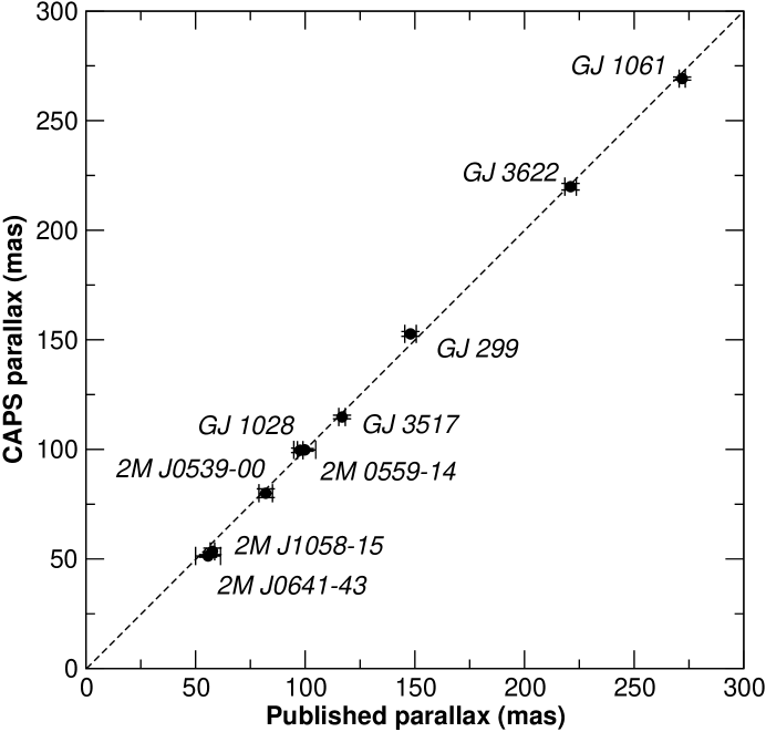
Figure 2: Comparison of the previously published parallaxes to a the CAPS program targets with more than 10 epochs. The published parallaxes have been obtained from SIMBAD (http://simbad.u-strasbg.fr/simbad/) and references therein.

Our measurement of GJ 317’s proper motion is similar to some previous estimates (e.g. Salim & Gould, 2003), which is another consistency check of the astrometric calibration procedure (e.g., plate scale and absolute field rotation). However, such proper motion is also relative to the references and requires more assumptions than the parallax zero-point to be properly corrected. For galactic kinematic studies, the catalog values of the proper motion given in Salim & Gould (2003, NLTT) or Zacharias et al. (2009, UCAC3) should be used instead of our relative measurement (see Table 2). Our relative proper motions in R.A. and Dec. agree within 15 and 2 mas yr^-1 to the values given in both these catalogs. Even though they differ by more than 1-$\sigma$ (statistical uncertainty), a discrepancy at the level of 15 mas yr^-1 is still acceptable due to the unknown zero-point in our relative measurements and the uncertainty in the catalogs themselves (random errors but also zonal systematic effects). GJ 317’s proper motion is also given in other catalogs; e.g. Roeser et al. (PPMXL 2010) and Monet et al. (USNO-B1.0 2003). We find that those measurements are unreliable. For example, the values given in PPMXL differ by 560 and 1350 mas yr^-1 from our measurement. A similar discrepancy is observed in USNO-B1.0, which is expected given that PPMXL is derived from USNO-B1.0. Given that the field is moderately crowded, we suspect that such mismatch is due to a crossmatching error (two stars with large proper motions are reported within 10^″ of the nominal position of GJ 317 in both catalogs). Even though GJ 317 is bright in the nIR, it can be easily confused with background objects at visible wavelenghts.

In summary, the measured trigonometric parallax of GJ 317 is 65.3$\pm$ 0.5 mas. This puts the star at a distance of 15.3 $\pm$ 0.2 pc compared to the value used by JB07 ($110\pm 20$ mas or 9.1$\pm$ 1.6 pc) using Jenkins (1963) and Gliese & Jahreiß (1991)). The other most recent measurement is 94.2 $\pm$ 12 mas (van Altena et al., 1995), still off by more than 2-$\sigma$ illustrating that previous parallactic measurements with uncertainties larger than 10 mas have to be taken with caution. Unfortunately, the astrometric amplitude due to an unseen companion is inversely proportional to the distance to the Sun. This effectively suppresses the expected astrometric signal by a factor of 1.7, providing a minimum (edge-on) semiamplitude of only 0.30 mas (compared to the 0.58 mas initially expected). The analysis and the actual limits imposed by the astrometry are discussed in Section 4.

Table 2: Properties of GJ 317.

Parameter	Value
$\mu_{R.A.}$ (mas yr-1)	-438 $\pm 5$
$\mu_{Dec.}$ (mas yr-1)	794 $\pm 5$
Absolute parallax (mas)	65.3 $\pm$ 0.4
$d$ (pc)	$15.10\pm 0.22$
Calan-ESO spectral type	M2.5V
$\left[\rm{Fe/H}\right]$	0.36 $\pm$0.2
$T_{\rm eff}$ (K)	$3510\pm 50$
	(fit to Baraffe+ 1998)
Adopted $M_{*}$ (M☉)	$0.42\pm 0.05$
Heliocentric RV (km s-1)	87.8 $\pm$ 1.5
Heliocentric UVW (km/s)	(-92.7, -52.5, 26.5)
Galactic UVW (km/s)	(-82.3, 178.3, 33.8)

2.1 Observations : Radial velocities

The 37 RV measurements presented herein were obtained with the HIRES spectrometer (Vogt et al., 1994) of the Keck I telescope from January 2000 to March 2010. This adds 18 measurements to those presented in the discovery paper of GJ 317b/c (Johnson et al., 2007). Typical exposure times on this star are 500 sec. The Doppler shifts are measured by placing an iodine absorption cell ahead of the spectrometer slit in the converging f/15 beam of the telescope. This gaseous absorption cell superimposes a rich forest of iodine lines on the stellar spectrum, providing a wavelength calibration and proxy for the point-spread function (PSF) of the spectrometer. For the Keck planet search program, we operate the HIRES spectrometer at a spectral resolving power R = 70,000 and wavelength range of 3700-8000 A, though only the region 5000-6200 A (with iodine lines) is used in the present Doppler analysis. Doppler shifts from the spectra are determined with the spectral synthesis technique described by Butler et al. (1996). Due to several improvements in our RV extraction pipeline for M-dwarfs (see Vogt et al., 2010, for further details), the new RV measurements update those given in Johnson et al. (2007). The HIRES/Keck has a demonstrated long term stability better than 3 m s^-1 for other stars with similar spectral types (e.g., Vogt et al., 2010). The analysis of the RV data is given in Section 4.1. The differential radial velocity measurements of GJ 317 are given in Table 3 and the average heliocentric radial velocity is given in Table 2. While the astrometry does not show any obvious signal, GJ 317b can be clearly seen in the RV data. The signal of GJ 317c is seen as a long term quadratic drift in the Doppler measurements (see Section 4.1).

Table 3: Differential radial velocity measurements of GJ 317 corrected by the barycentric motion of the observer

Julian date	RV	Uncertainty
(days)	(m s-1)	(m s-1)
2451550.99259	7.34	3.73
2451552.98958	21.52	5.07
2451582.89062	49.03	4.05
2451883.10117	-24.37	3.70
2451973.79513	-68.35	6.28
2452243.07296	0.00	6.64
2452362.94880	84.76	6.20
2452601.04502	-39.89	5.19
2452989.12482	102.30	5.21
2453369.01627	-37.70	3.55
2453753.98281	128.09	3.45
2454084.00126	-19.25	4.65
2454086.14134	-24.09	4.75
2454130.08245	-16.49	5.35
2454131.01418	-12.56	4.71
2454138.93219	-15.19	3.01
2454216.73300	1.08	4.20
2454255.74588	18.98	2.41
2454400.10995	117.38	3.93
2454428.06242	128.31	4.59
2454464.99786	116.58	4.27
2454490.95016	119.13	5.09
2454492.90113	115.61	4.11
2454543.94829	90.23	4.87
2454544.90468	95.00	3.52
2454545.89435	95.14	3.79
2454600.82150	54.64	4.75
2454806.02892	-13.08	3.99
2454807.06907	-16.41	6.62
2454808.13819	-17.69	3.53
2454809.05881	-25.66	3.48
2454810.16094	-28.96	3.75
2454811.12802	-23.48	3.61
2454820.95173	-12.90	2.78
2454822.98435	-8.78	2.77
2454839.10383	-29.39	4.46
2455258.83718	92.12	4.74

3 GJ 317 is a metal rich M dwarf

GJ 317 (LHS 2037) was classified as an M3.5V star based on similarities to the high resolution spectrum of the M3.5V M dwarf GJ 849 (JB07). The assumed distance was 9.1 pc. In JB07, it was noted that the photometry looked anomalous in the sense that the magnitudes did not match those expected for a main sequence star. The comparison star(GJ 849) has a HIPPARCOS parallax (van Leeuwen, 2007) also giving a distance of 9.1 $\pm$ 0.2 pc. Therefore, if both stars were of the same spectral type, they should exhibit similar magnitudes. This is clearly not the case (on average, GJ 317 is 1.5 magnitudes fainter in all the bands as given by the Simbad) compilation. Rojo & Ruiz (2003) used photometry and low resolution spectroscopy to obtain a spectral type of M2.5V, but reported a photometric distance estimate of 7 pc, which puts the star even closer. As we show in this section, the updated distance (15.3 pc) and, high metallicity seem to solve most of these apparent contradictions.

Table 4: Photometry of GJ 317. Absolute magnitudes assume a distance of 15.3 $\pm$ 0.2 pc.

Band	Measured	Absolute
B	13.48 $\pm$ 0.03	12.56 $\pm$ 0.04
V	11.98 $\pm$ 0.03	11.06 $\pm$ 0.04
R	10.82 $\pm$ 0.03	9.89 $\pm$ 0.04
I	9.32 $\pm$ 0.03	8.39 $\pm$ 0.04
J	7.934 $\pm$ 0.03	7.01 $\pm$ 0.03
H	7.312 $\pm$ 0.07	6.39 $\pm$ 0.08
Ks	7.028 $\pm$ 0.02	6.10 $\pm$ 0.03

Given a trigonometric distance, the mass and temperature of GJ 317 can be obtained by fitting the absolute magnitudes to the theoretical models given by Baraffe et al. (1998). Table 4 shows the available photometry of GJ 317 (B, V, R, I, J, H and K_s) and the updated absolute magnitudes. The adopted photometric measurements in the visible are those given by Rojo & Ruiz (2003). The infrared magnitudes have been taken from the 2MASS catalog (Skrutskie et al., 2006). Even though there are other photometric measurements in the literature, most of them agree within the reported uncertainties. The fit is obtained by adjusting the absolute magnitudes to the values tabulated in Baraffe et al. (1998), using the temperature as the only free parameter. Because the star has low activity levels and low $v\sin i$ (JB07), we assume an age of 5 Gyr (M dwarfs change their colors very little after 1 Gyr). This fit leads to a preliminary mass of $M=0.38$ M_☉ and an effective temperature of T_eff = 3510 K. If only infrared colors are used (J, H and K), a slightly hotter and more massive star is recovered; T_eff = 3550 K and 0.43 M_☉. As can be seen in Fig. 3, the predicted flux in the optical wavelength range is still overestimated by the models; that is, the star seems to be fainter than expected in the bluer colors. While moderate interstellar absorption by dust could be the cause, GJ 317 is a relatively nearby star and there is no reported evidence of strong extinction in its direction. A_V is 0.3 mag for the whole integrated galaxy in the direction of GJ 317, and still would be insufficient to explain the observed excess. The absolute magnitudes can also be used to infer the mass of GJ 317 using the empirical relations given by Delfosse et al. (2000). From the absolute J, H, and K_s magnitudes we obtain : $M_{*J}=0.41M_{\sun}$, $M_{*H}=0.42M_{\sun}$, $M_{*K}=0.43M_{\sun}$, while using V and V-K, we derive $M_{*V}=0.37M_{\sun}$ and $M_{*V-K}=0.25M_{\sun}$. These mass estimates show a similar trend as the fit to the theoretical models: longer wavelength photometry favor larger masses. As advised by Delfosse et al. (2000), we adopt the average of the masses obtained from the JHK magnitudes ($M_{*}=0.42M_{\sun}$) as the most reliable estimate. This value is 1.75 times larger than the one adopted by JB07 in the discovery paper of GJ 317b and c. Therefore, the derived minimum masses for both planets will be increased accordingly (see Section 4.1).

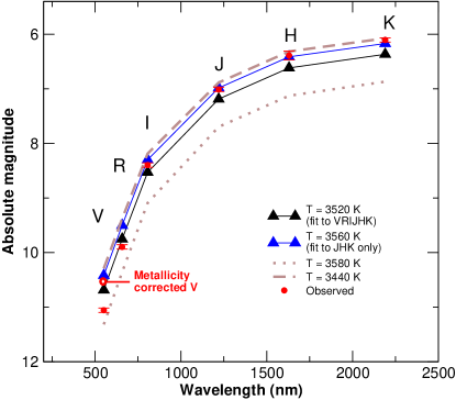
Figure 3: Fit of the VRIJHK magnitudes to the Baraffe et al. (1998) theoretical models (black triangles). Compared to the models, the Visual V mangitude is fainter and the J,H,K colors appear brighter than expected by many standard deviations. A fit only to the JHK magnitudes is shown in blue triangles. A much better agreement is recovered when the V magnitude is ’corrected’ by its metallicity (see text).

Metallicity has an effect on the colors of M dwarfs: a star with super-solar metallicity will have the V-band flux suppressed compared to a star of the same spectral type with solar metallicity. This effect has been used to estimate metallicities of field M dwarfs, so it would not be surprising that the visual mangitudes appear fainter than expected if GJ 317 were, in fact, metal rich. The best calibrations use the V-K color against the absolute K magnitude to estimate [Fe/H] : Bonfils et al. (2005) or B05, Johnson & Apps (2009) or JA09, and Schlaufman & Laughlin (2010) or SL10. All three calibrations are empirical and are based on measured metallicities of nearby stars with good parallax measurements. Based on the previous distance, JB07 obtained a [Fe/H] = -0.23. This value made GJ 317 the only ’metal poor’ M dwarf with detected giant planet candidates. Given the updated M_K, all three methods now indicate that the star is indeed metal rich ([Fe/H]= +0.08 for B05, [Fe/H] = +0.43 using JA09, and [Fe/H] = +0.29 using SL10). Since B05 tends to underestimate metallicities (Johnson & Apps, 2009; Rojas-Ayala et al., 2010), we adopt the average of the JA09 and SL10 calibration, i.e. 0.36, as the updated value for [Fe/H].

We now investigate whether or not the color/metallicity relation can explain the apparent extinction in the visible magnitudes when compared to the models or to the mass/luminosity relations. Since the highest metallicity comes from the JA09 calibration, and assuming that $M_{\rm K}$ is correct, we ask what V magnitude would be required to conclude that the star has [Fe/H] = 0.0 (this is the metallicity assumed by the Baraffe et al. (1998) models). By iterating on the JA09 relation we find that V=11.45 (compared to an observed V=11.98) gives zero metallicity. We can now test whether this value can do a better job fitting the theoretical models. We find that the correction is in the right direction (see Fig. 3) and it significantly improves the fit to the V, J, H and K photometry. Also, the revised mass derived from the models is now 0.42 $M_{\sun}$, much closer to the one fitting the J, H and K bands only ($0.43M_{\sun}$). Moreover, if we apply the mass/luminosity relations in Delfosse et al. (2000) to the ’corrected’ V magnitude, we obtain $M_{*V}=0.43M_{\sun}$ and $M_{*V-K}=0.41M_{\sun}$, now in perfect agreement with the value obtained from J, H and K. A similar behaviour would be expected for the R and I bands, but no empirical color metallicity relations have been published on these bands. Delfosse et al. (2000) already mentioned that the mass/luminosity relation using the V color has an excess of dispersion due to the unknown metallicities of M dwarfs. The remarkable agreement in all the quantities recovered after ’correcting’ V for the effect of metallicity seems to confirm this. As a more definitive proof, it would be desirable to obtain a direct metallicity measurement using the newly developed spectroscopic methods in the near infrared (e.g., Rojas-Ayala et al., 2010).

Given the new distance measurement, we can re-compute its tangential and galactic 3D velocity to check whether GJ 317 could be a member of a known kinematic group. The UVW velocities in the Heliocentric and the Galactic reference frames are given in Table 2. The resulting U and V components are large but not unusual for disk stars. We have integrated the Galactic orbit using a basic potential for the Galaxy (thin disk, thick disk, bulge and halo, see Paczynski (1991)) and a 4th order Runge-Kutta integrator (time steps of 100 years). We find that past and future trajectories lie well within the galactic disk region. Actually, a large U component with a V component of the order of $\sim-50$ km/s and a moderate W are typical of a thick disk population member (see Fig. 1 in Bensby et al., 2007). This would be consistent with the star being old ($>3$ Gyr) and inactive. Even though the boundaries between thick and thin disks are diffuse (Bensby et al., 2007), everything indicates that it is a likely a member of the Galactic thick disk population.

In summary, the previously reported anomalies in the photometry of GJ 317 seem to be related to the previous poor estimate of its distance and its high metal content. The new metallicity determination strengthens the observed correlation of super solar metallicity and the presence of giant planets around M dwarfs (Rojas-Ayala et al., 2010; Johnson & Apps, 2009).

4 Orbital analysis

At the updated distance, our astrometric measurements cannot resolve the wobble of planet b (minimum amplitude $\sim 0.3$ mas). Assuming an epoch-to-epoch precision of 0.9 mas (average between R.A. and Dec. precisions) on 18 epochs and Gaussian statistics, an amplitude of 0.30 mas should be detected only with a signal-to-noise ratio of 1.4. An amplitude of 0.65 mas should be detected with a SNR of 3 if present. Therefore, at our present precision the amplitude of the signal can only be marginally measured with a signal-to-noise ratio between 1 and 4 (depending on the actual orbital inclination). While this is insufficient to obtain an unambiguous detection, our analysis shows that we can actually put tight constraints on the mass of GJ 317b, thus confirming its planetary nature. Because of the reduced sensitivity of the astrometry, the orbital parameters constrained by the RV are not sensitive to the astrometric measurements. Therefore, we first provide a detailed analysis of the RV data and then we discuss the constraints imposed by the astrometric measurements on GJ 317b and GJ 317c.

4.1 RV analysis

We use the latest stable version of the systemic interface (Meschiari et al., 2009, v1.5.12) to obtain the best fit to the RV data. GJ 317b is clearly seen in the periodogram as a strong peak around 700 days. After subtracting the best orbital fit for GJ 317b (see Table 5), a long term trend is still apparent in the residuals. Assuming a circular orbit we obtain a period of 7100 days for GJ 317c. Even in the circular orbit case, a broad range of periods and masses are still allowed by the data. For an eccentric solution ($e_{c}\sim 0.81$), the most likely period falls between 50 000 and 90 000 days ($\sim$ 130–250 years). Compared to the orbital solution of JB07 based on 18 measurements, it is now more clear that a constant slope is insufficient to reproduce the observed RVs and that the curvature of the orbit is clearly detected in the data. In the case of eccentric orbits, such long period signals can only be detected if the planet is close to the periastron of its orbit, which might be the case here. In any case, several more years of RV measurements will be required to put a more significant constraint on this orbit.

Table 5: Orbital solution for GJ 317b/c from the RV data only. All parameters are referred to the initial epoch $T_{0}$=2451550.9925. The mass of GJ 317 is assumed to be 0.42 M_☉.

	GJ 317b	GJ 317c	GJ 317c
		(circular)	(eccentric)
$P$ (days)	692 $\pm$ 2	7100${}^{+8000}_{-1500}$	$>10^{4}$
$K$ (m s-1)	73.5$\pm$ 2	30.5 $\pm$ $5$	$\sim$ 30
$e$	0.11 $\pm 0.05$	0 (fixed)	0.81 $\pm$ 0.2
$M_{0}$	309 $\pm$ 15	199${}_{-25}^{+75}$	350
$\omega$ (deg)	340 $\pm$ 10	–	210
$\gamma$ (m s-1)		18	40
Derived quantities
$M\sin$ i ($M_{jup}$)	1.81 $\pm$ 0.05	1.6	$\sim$2.0
a (AU)	1.148	5.5 AU	10-40 AU
Statistics
NRV		37	37
RMS (m s-1)		8.5	7.3
$\chi^{2}_{RV}$		4.97	4.36

We find that the orbital solution for GJ 317b remains well constrained irrespective of the orbital fit to GJ 317c. We use a Bayesian Monte Carlo Markov Chain (MCMC) approach to characterize the probability distributions of the free parameters and get a realistic estimate of their uncertainties. The methodology applied to obtain such distributions is described in Appendix B. Using only RV observations, we find that the orbit of planet b is well constrained in a narrow region of the parameter space, while the period and eccentricity of planet c still have broad probability distributions (the 99% confidence level interval allows 20 $<$ P $<$ 240 years if the orbit is allowed to be eccentric). These broad distributions are caused because planet c is only detected as a secular quadratic term that can be reproduced by many combinations of parameters (see Gould (2008) for a detailed discussion of the problem). The best fit orbital solutions for GJ 317b and GJ 317c are shown in Table 5. The uncertainties were obtained using the aforementioned MCMC technique and represent the 68% confidence level intervals around the least-squares solution. Note that, because the mass of the star has been updated, the minimum mass of planet b (1.8 $M_{Jup}$) is larger than the value given by JB07 (1.2 $M_{Jup}$).

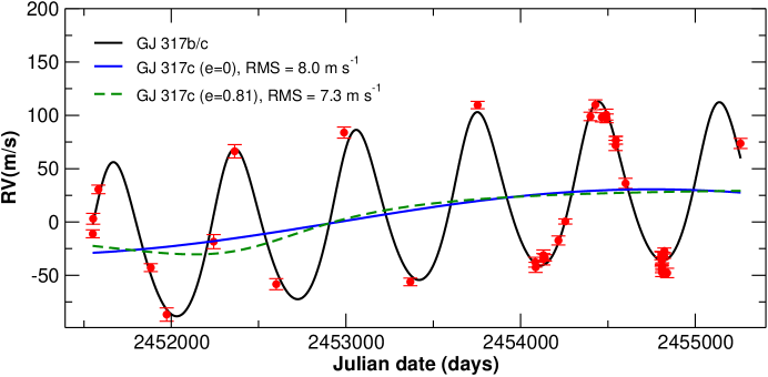
Figure 4: Best orbital fit to the RV data, assuming an eccentric orbit for planet GJ 317c (solid black line). The signal of GJ 317c can be seen in the secular trend of the RV signal of GJ 317b. We overplot the signal of GJ 317c assuming a circular orbit (solid blue) and the best eccentric orbital fit (dashed green).

After removing both signals, there is no conclusive indication of additional planets in the RV data. However, the root mean squared (RMS) of the residuals ($\sim$8 m s^-1) is significantly larger than that expected from observations of similar stars without planets (RMS $\sim$ 3 m s^-1, see Section 2.1). Also, the short period domain (a few days to weeks time scales) is still poorly sampled. Given the abundance of low mass objects in multi–planet systems (Howard et al., 2010), additional low mass companions might be expected to emerge as more RV measurements are obtained.

4.2 Astrometry and radial velocities

To perform a joint fit of the astrometry and the RVs, we subtract the best orbital solution for planet c (e = 0.81), leaving only the RV signal of GJ 317b in the RV data. The least-squares solution for the combined astrometry and radial velocities is obtained on a grid of fixed period/eccentricities around 690 days (50 test periods between 680 days and 700 days and 20 test eccentricities from 0 to 0.95). All the other parameters are left free. In a last step, the period and the eccentricity are refined starting at the best solution on the grid. The best fit values (see Fig. 5 and Table 6) are then used to initialize a Bayesian Monte Carlo Markov Chain sampler to generate again the a posteriori probability distributions, including now both the RVs and the astrometry in the definition of the likelihood function. The condition equations that the astrometry and the radial velocities have to satisfy together with a brief explanation of the Bayesian MCMC method are given in Appendix B. The same analysis procedure was also used in Anglada-Escudé et al. (2010) to combine astrometric and RV measurements and rule–out the existence of the astrometric planet candidate VB10b, at least in moderately eccentric orbits. As in the RV analysis, the steps in the Markov Chain sampler are tuned to accept 15% to 30% of the proposed updates, and the first 10⁵ steps are not used in the analysis to avoid oversampling the favoured solution. Chains with 5$\times$10⁶ steps are used to generate the numeric realization of the a posteriori distributions for all the parameters. We repeat the process several times and compare the resulting distributions to be sure that the chains are properly converged obtaining good agreement in all the runs.

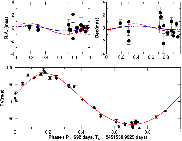
Figure 5: Best fit astrometry + RV joint solution for GJ 317b. Top panels are R.A. and Dec. as a function of time. The dashed–red line corresponds to the signal of a 4.0 $M_{Jup}$ mass planet. The dotted–red line corresponds to the signal of a planet with the minimum mass allowed by the radial velocities (1.8 $M_{Jup}$). The best fit solution is plotted as a blue line. Bottom panel: the radial velocity data plotted with the best fit solution after removing the signal of planet c.

The best fit solution (maximum likelihood values) with the corresponding 68% confidence level intervals are given in Table 6. Flat prior distributions have been used in all the cases. Figure 6 shows the final probability distributions for the two parameters that the astrometry can constrain. The fact that the signal is barely detectable bodes ill for the determination of the argument of the node (upper panel). However, with a 99% confidence level, the inclination is constrained to be greater than 25 deg (see bottom panel in Figure 6) because a value lower than that would result in a wobble that is not seen. The top panel in Figure 7 illustrates the distributions for the mass and the argument of the node. The distribution for the mass of GJ 317b is clearly non-Gaussian due to the strong lower limit imposed by the RV data on the minimum mass and the more loose constraints imposed by the astrometry on the maximum allowed signal. The bottom panel of Figure 7 shows the histogram of the probability distribution for the mass. Note that an inclination closer to 0 would have two effects : first, the amplitude grows as $1/\sin i$, and second, as the orbit becomes face on, the amplitude becomes more ’2-dimensional’. This is, an edge-on orbit would be seen as a line, while a face-on orbit (inclination close to 0) would show up as a circle increasing its statistical significance. To obtain the range of allowed masses, the obtained MCMC distribution can be numerically integrated from $M$ to $\infty$ (shaded histogram in bottom panel of Figure 7). We find that the probability of $M>3.6M_{jup}$ is only 1%. This value is much lower than 13 $M_{\rm jup}$ (approximate planet/brown dwarf boundary) and unambiguously confirms that GJ 317b is an actual planet.

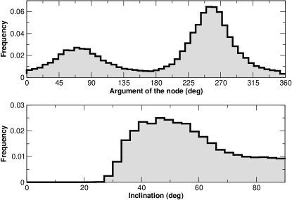
Figure 6: Bayesian probability distributions for the orbital parameters constrained by the astrometry observations. Because the signal is only marginally detected, the argument of the node is poorly constraint. A robust lower limit for the inclination is obtained.

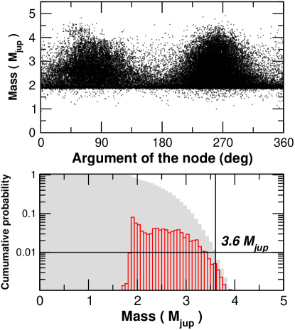
Figure 7: Top. Markov Chain results illustrating the probability distribution of the argument of the node of GJ 317b plotted against the mass (only one of every 100 steps is shown to improve visualization). Bottom. In red we show a histogram of the marginalized distribution for the mass of GJ 317b. The cumulative probability for the maximum mass of GJ 317b is shown in grey. The RV data acts as a strong prior (abrupt cut below 1.8 $M_{Jup}$), effectively suppressing solutions below the minimum mass. The upper limit on the mass is set by the astrometry at 3.6 $M_{jup}$.

Table 6: Best orbital Solution for GJ 317 b. All parameters are referred to T₀=2451550.9925.

RV observables		Astrometric observables
$P$ (days)	692 $\pm$ 2	Relative $\mu_{R.A.}$ (mas/yr-1)	-457.8 $\pm$ 0.5
$K$ (m s-1)	75.2 $\pm$ 3.0	Relative $\mu_{Dec.}$ (mas/yr-1)	796.5 $\pm$ 0.5
$e$	0.11 $\pm$ 0.05	Relative parallax (mas)	65.0 $\pm$ 0.4
$M_{0}$ (deg)	305 $\pm$ 15	$\Omega$ (deg)	82
$\omega$ (deg)	342 $\pm$ 10	$i$ (deg)	45 ${}^{+30}_{-10}$
Statistics		Derived quantities
NRV	37	$P$ (years)	1.894 $\pm$ 0.013
Nastro	17 $\times$ 2	$M$ $\sin i$ (Mjup)	1.8 $\pm$ 0.05
RMSRV (m s-1)	7.4	$M$ (Mjup)	2.5${}^{+0.7}_{-0.4}$
RMSR.A. (mas)	0.70	$a$ (AU)	1.15 $\pm$ 0.05
RMSDec. (mas)	1.23	Angular separation (mas)	76
TP (Julian date)	2451656.7 $\pm$ 35
$\chi^{2}_{RV}$/NRV	3.1
$\chi^{2}_{R.A.}$/Nastro	1.1
$\chi^{2}_{Dec.}$/Nastro	4.8

Bayesian methods are very sensitive to the correct estimation of the single measurement uncertainties, so we performed a few additional tests to check the robustness of the upper limit found for the mass. First, we repeat the whole process (least-squares grid + MCMC) assigning a constant 1 mas uncertainty to weight each measurement. The actual maximum mass at the 99% confidence level (C.L.) is a bit larger (3.8 $M_{jup}$). This comes from the fact that we are effectively downgrading the confidence in the R.A. measurements, which are the more constraining ones. We also tried shuffling the residuals in the astrometry and then repeating the orbit fitting process on the shuffled sets. We find a slightly larger upper limit on the mass of the shuffled sets ($\sim 4M_{Jup}$) than on the real data, confirming that the signal is just barely resolved by the astrometry, probably only in R.A. The bias towards low inclinations (large dynamical masses) in the presence of noise is a known effect in the analysis of astrometric observations (Pourbaix & Arenou, 2001). Therefore, the upper limit we find to the mass of GJ 317b is a very robust result.

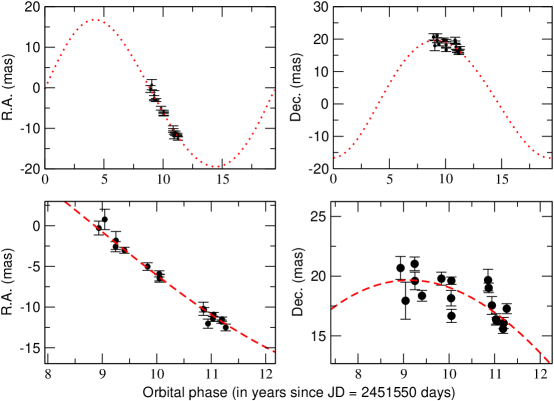
Figure 8: Top panels : Best orbital solution using the astrometry on planet GJ 317c. Bottom panels : Zoom-in on the orbit as sampled by the CAPScam astrometry. Because it has a very long period, the signal is mostly a linear trend that cannot be de-coupled from the proper motion yet (Black & Scargle, 1982). In 3 to 4 years, the acceleration should be obvious in (at least) one of the directions.

We also tested if the astrometry could put constraints on the inclination and the mass of the outer planet c. To do this, we removed GJ 317b from the radial velocities and combined the astrometry and the radial velocities in a Bayesian MCMC initialized at the best circular orbit from the RV. This time, because the period is so long, the eccentricity is poorly constrained and because there is no appreciable acceleration in the astrometry (see the residuals in Fig. 1), the true mass of the companion is still very uncertain. We note that if a linear trend in the astrometry were large enough to be detected, then this trend would be absorbed by the fit to the proper motion. This is a known issue for astrometric planet detection and was first discussed by Black & Scargle (1982). Assuming a circular orbit, masses up to 22 $M_{Jup}$ are still compatible with the astrometry (at a 99% C.L.) If the orbit is allowed to be eccentric, masses up to 200 $M_{Jup}$ are still allowed on orbits close to face-on. We anticipate that, at least, 3-4 more years of follow up will be necessary to obtain a first hint of the astrometric acceleration (see Figure 8) and put a meaningful constraint on the mass of GJ 317c. Depending on the actual age of the system, direct imaging of GJ 317c might be achievable with state-of-the-art high contrast imaging systems(e.g., Lagrange et al., 2010). Imaging combined with RV and astrometric measurements will provide a direct measurement of the mass of the planet and the mass of the star.

5 Discussion

We have obtained precision astrometric measurements of the M dwarf GJ 317 and combined these with new radial velocities. Even though the signal is not fully resolved by the astrometry, the new measurements put meaningful constraints on the mass of GJ 317b, confirming its planetary nature. Combining astrometric and radial velocity measurements is a complex multi-parametric problem where the final probability distributions for the involved parameters are not necessarily Gaussian. This upper limit has been obtained using a Bayesian MCMC approach which is much better suited than a classical $\chi^{2}$ analysis to put contrains on parameters and obtain confidence intervals. Given that the upper limit to the mass of GJ 371b ($\sim 3.6M_{jup}$) is much lower than the planet/brown dwarf boundary, it is the first time ground-based astrometric observations have been able to confirm the planetary nature of a substellar companion. The presented radial velocities confirm the presence of an extremely long period planet (period 20 years or more) that is not yet detected in the astrometry.

Other RV surveys (e.g., Zechmeister et al., 2009; Johnson et al., 2007) have found a low occurrence rate of moderate–to–short period gas giants around M dwarfs, with the resonant pair GJ 876b/c the only remarkable exception (Rivera et al., 2010). No hot Jupiters (P$<$30 days) have been reported around a low mass star. A handful of gas giants with periods longer than 30 days have been found around a few early type M dwarfs (e.g. GJ 179b, GJ 832b, GJ 849b, HIP 79431b, HIP 57050b, see the exoplanet encyclopedia for an up-to-date list). This seems to indicate that M dwarfs have trouble forming and/or keeping giant planets in tight orbits.

According to recent studies, the frequency of M dwarfs hosting gas giants seems rather low compared to more massive solar type stars (e.g. Johnson et al., 2010). This is an expected consequence of the core accretion model for giant planet formation Laughlin et al. (2004); Kennedy & Kenyon (2008); Alibert et al. (2011). Also, the new distance measurement indicates that GJ 317 is metal rich. With GJ 317 now in the club, all the M dwarfs with reported giant planets are metal rich (Rojas-Ayala et al., 2010; Johnson & Apps, 2009). The competing mecanism model for planet formation (Boss, 1997, disk instability model) should not be very sensitive to the metallicity of the host star, so this has also been suggested as evidence in favor the core-accretion scenario (e.g.,see Ida & Lin, 2004; Mordasini et al., 2009). However, core accretion is still too slow to form long period gas giant planets around low mass stars, except for exceptionally long lived disks (Ida & Lin, 2005). Also, core-accretion fails to reproduce the over-abundance of planets in close-in orbits around all stellar types found by Kepler/NASA (Borucki et al., 2011). On the other hand, disk instability is able to form gas giants around M dwarfs with short lifetime disks (Boss, 2006, 2011). Given these two issues (time-scale problem and incorrect prediction of the observed planet distributions), we find it more natural to invoke the disk instability mechanism to explain the formation of GJ 317c, and possibly GJ 317b as well. Given that the number of nearby M dwarfs surveyed for planets is still small, more detections in a statistically larger sample are required to put real constraints on the metallicty-gas giant connection. This is one of the long term goals of the Carnegie Astrometric Planet Search project.

GJ 317 is one of the faintest targets in the Lick-Carnegie planet search program, and precision radial velocities in the optical are limited by photon noise and require intensive use of large aperture telescopes (Keck/HIRES) to reach the few m/s precision level. Since it is a cool star (T$<$4000 K), most of its flux is in the near infrared; so it will be an excellent target for precision RV measurements when the new generation of near infrared spectrographs comes on-line (Bean et al., 2010; Figueira et al., 2010; Anglada-Escudé & Plavchan, 2011). Also, the star lies in the optimal magnitude range (12$<$V$<$15) for the Gaia/ESA space astrometry mission (Lindegren, 2010) and the PRIMA/VLT interferometer (Koehler et al., 2010). Both instruments will have a single measurement precision better than 0.1 mas and the orbit of GJ 317b (minimal semiamplitude of 0.3 mas) will be clearly resolved once an orbital period ($\sim$ 700 days) is covered. Since the astrometric signal of the long period planet GJ 317c should be evident in a few more years of CAPScam observations as a quadratic term, we will continue monitoring this star at lower cadence to measure its orbital inclination and mass.

Finally, we highlight some unique features of GJ 317. It is a relatively bright, low mass star with super solar metallicity, so it seems an ideal target to look for low mass terrestrial planets in its habitable zone. Recent studies (Mayor et al., 2009; Howard et al., 2010) indicate that 30% of the dwarf stars host planets in the super-earth mass range. This fraction seems to be even higher in multi-planetary systems. Such planets in the habitable zone around GJ 317 should have orbital periods of a few weeks and RV amplitudes of several m s^-1. The fact that the system contains a pair of long period giants might have helped to deliver volatile compounds to the inner orbits as seemed to have happened in the early Solar System (Crida, 2009). On the other hand, significantly eccentric orbits are possible for both outer planets, which might be a problem for the long term stability of the inner orbits (Chambers & Cassen, 2002). Finally, the outermost giant planet might be detectable by direct imaging in the near future (e.g. Lagrange et al., 2010, found a sub stellar companion to $\beta$ Pic at a similar angular separation). An image of this planet combined with the astrometry and the RV would provide a model independent measurement of its mass. In summary, in a few years GJ 317 might become one of the better characterized planetary systems beyond our own.

Acknowledgements. G.A. gratefully acknowledges the support of the Carnegie Postdoctoral Fellowship program. G.A. also thanks Cassy Davison and Todd Henry, both at Georgia State Universtity, for valuable comments and discussions. A.P.B., A.J.W. and G.A. gratefully acknowledge the support provided by the NASA Astrobiology Institute grant NNA09DA81A, and the continuous support of the Carnegie Observatories TAC to the CAPS program. R.P.B. gratefully acknowledges support from NASA OSS Grant NNX07AR40G, the NASA Keck PI program, and from the Carnegie Institution of Washington. S.S.V. gratefully acknowledges support from NSF grant AST-0307493. Some of the work herein is based on observations obtained at the W. M. Keck Observatory, which is operated jointly by the University of California and the California Institute of Technology, and we thank the UC-Keck and NASA-Keck Time Assignment Committees for their support. The Lick–Carnegie group members acknowledge the contributions of fellow members of our previous California Carnegie Exoplanet team in helping to obtain some of the earlier RVs presented in this paper.

Facilities: Du Pont (CAPScam), Keck:I (HIRES)

Appendix A The ATPa pipeline : Astrometric extraction, calibration and solution

The reduction of the astrometric observations is done using the ATPa software, specifically developed for the CAPS project . Further details on the various steps of the astrometric data reduction are given in Boss et al. (2009). The astrometric processing done by ATPa can be outlined as follows. First, the position of all the stars in each image is extracted and mapped to a tanget plane to the sky centered at the nominal coordinates of the target star at the first epoch of observation. For each image, a subset of reference stars are matched to their predicted position to adjust the telescope pointing, plate scale, rotation and fit for a geometric field distortion. These predicted positions are initialized using the stars extracted from a high quality image. Using this image-by-image solution, the position of each star in the field is mapped to the frame defined by the reference stars. Then, all the measured positions in a night (or epoch) are averaged to obtain the epoch position and its uncertainty of each star in the field. Finally, all the epochs are fitted to a linear astrometric model (position, proper motion and parallax) and the reference frame is refined by selecting those stars showing the smallest residuals. This process is iterated a few times untill convergence is reached, this is, when the root-mean-squared (RMS) of the residuals of the reference stars does not change significantly (e.g. less than 0.05 mas). We call this process the astrometric iterative solution (or AIT). The result is a catalog of positions, parallaxes and proper motions for all the stars in the field.

Now let’s describe each step in more detail. The centroids of the stars are measured by binning the stellar profile in the X and Y directions on a box of 12 pixels ($\sim 2\arcsec$) around the pixel with maximum flux. This one dimensional profile is then precisely centroided using a function called Tukey’s biweight function(see p. 448 on Tukey, 1960). Many simulations and tests with different profiles showed that this approach provided the best centroid accuracy and robustness (see Boss et al., 2009, for further details). The flux is also measured on a circular apperture of 10 pixels around the obtained centroid and the sky obtained from a ring of 15 to 20 pixels is then subtracted. As a result, each image produces a list of star positions and fluxes. A preliminary centroid accuracy for a given night is empirically obtained using a rough reference frame consisting on the the best 10 stars in the field in terms of centroid nominal precision. Finally, the nominal optical distortion of CAPScam is used to map the pixel positions to a local tangent planet to the sky. This nominal field distortion was obtained in April 2011 by observing a moderately crowded field on a rectangular grid of 16 positions spaced by 40$\arcsec$ (North–East tip of the rectangle centered at 16:00:11.41 -40:12:42.2). This method of measuring the nominal optical distortion is described in Anderson (2007) and references therein.

To initialize the astrometric iterative solution, the extracted positions of one image are used as a template to generate an initial catalog. In this first iteration, all the images are matched to this catalog using a linear distortion model. This is, assuming that the predicted local tangent plane position of the i-th reference star is ($u_{i}$, $v_{i}$), the geometric calibration consists in finding the coefficients that satisfy

$$u_{i} = a_{0}+a_{x}x_{i}+a_{y}y_{i}\,,$$ (A1)

$$v_{i} = b_{0}+b_{x}x_{i}+b_{y}y_{i}\,,$$

where $x_{i}$ and $y_{i}$ are the extracted positions of the references obtained in the ONP step after applying the nominal CAPScam distortion. The same transformation is then applied to all the stars in the field. The nightly averaged $u$ and $v$ of each star is obtained (this is what we call an astrometric epoch measurement) and the intranight standard deviation divided by the square root of the number of observations is used as the associated epoch uncertainty (i.e. uncertainties in Table 1). Finally, all the epochs are used to update the astrometric solution for each star by fitting their motion to

$$u(t) = u_{0}+\mu_{\alpha}\left(t-t_{0}\right)-\Pi p_{\alpha}(t)+\Delta_{\alpha}\,,$$ (A2)

$$v(t) = v_{0}+\mu_{\delta}\left(t-t_{0}\right)-\Pi p_{\delta}(t)+\Delta_{\delta}\,,$$ (A3)

where $\mu_{\alpha}$ and $\mu_{\delta}$ are the proper motion in the direction of increasing R.A. and Declination respectively (in mas yr^-1), $\Pi$ is the parallax in mas, $u_{0}$ and $v_{0}$ are constant offsets (in mas) that provide the star position on the local plane at the reference epoch $t_{0}$ assuming zero parallax. The numbers $p_{\alpha}$ and $p_{\delta}$ are the so-called parallax factors and correspond to the parallactic apparent motion projected on the direction of increasing R.A. and Dec. at the observing instant $t$. To ensure maximal precision, the parallax factors are derived using the position of the geocenter from the DE405 JPL Ephemeris of the Solar System . Note that the 5 free parameters on this equation (u₀, v₀ ,$\mu_{\alpha}$,$\mu_{\delta}$ and $\Pi$) are linear. Therefore, the corresponding system of normal equations can be efficiently solved in a single least-squares step. The perspective acceleration for GJ 317 (Dravins et al., 1999) is negligible given the relatively short time baseline of this dataset ($\sim$ 0.042 mas over two years) and is not included in the processing. A simple derivation of this astrometric model and additional second order terms are outlined in Anglada-Escudé & Debes (2010). $\Delta_{\alpha}$ and $\Delta_{\delta}$ contain possible perturbations to the baseline astrometric model but they are not adjusted during the AIT. For the target star, $\Delta_{\alpha}$ and $\Delta_{\delta}$ will include the astrometric Keplerian motion following the prescriptions outlined in Appendix B.2. Such functions implicitly depend on the Keplerian parameters in a complicate non-linear fashion, specially when combining astrometric and radial velocity observations.

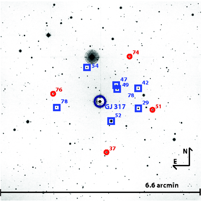
Figure 9: GJ 317 field of view as seen by CAPScam on March 18th, 2011. Reference frame stars are marked with circles and squares. Stars marked with blue squares are the ones used to derived the zero–point parallax. Stars marked as red circles are still used as references but could not be used to obtain the zero–point correction because one or more photometric bands required (B, J, H or K) were missing in NOMAD.

Because this field is particularly rich in stars, our sotfware is able to automatically select 11 very stable references within 120${}^{{}^{\prime\prime}}$ of the target. By stable we mean that the RMS of the epoch-to-epoch residuals (RMS) is smaller than 1 mas. In a second iteration, these 11 references are used to recompute the field distortion of each image with respect to the updated version of the catalog. This time, a second order distortion correction (6 coefficients are adjusted on each axis) is fitted to each image. This is,

$$u_{i} = a_{0}+a_{x}x_{i}+a_{x}y_{i}+a_{xx}x_{i}^{2}+a_{yy}y^{2}_{i}+a_{xy}xy\,,$$ (A4)

$$v_{i} = b_{0}+b_{x}x_{i}+b_{x}y_{i}+b_{xx}x_{i}^{2}+b_{yy}y^{2}_{i}+b_{xy}xy\,$$

The RMS of each star and the epoch uncertainty derived in the previous iteration are used to obtain a weighted solution of Eq. A4. A 3-$\sigma$ clipping of the outliers is also required to obtain a more robust determination of the field distortion. Finally, an updated version of the catalog is obtained by fitting Eq. A2 again to all the stars. Because the precise positions and motion of the references are not known a priori, the process has to be iterated a few times. The convergence criteria is that the average RMS of the references changes by less than 0.05 mas with respect to the previous iteration. For this field in particular, only 5 iterations were required to reach convergence. The astrometric solution for the reference stars and their catalog information (Zacharias et al., 2004) are given in Tables 7 and 8, and their distribution on the field of view of CAPScam is illustrated in Figure 9.

Appendix B Bayesian Monte Carlo Markov Chains

Bayesian statistics allow computation of the probability distributions of the free parameters constrained by a set of observations. The general strategy we use in this work is based on the methods described in full detail in Ford (2005), which we strongly encorauge to read. To obtain the parameter distributions compatible with the data we have to obtain the likelihood function which, in this case, is just the productory of the probability distributions of all the available observations. This is, assuming that the uncertainties in in the measurements follow a Gaussian distribution, the likelihood function $L$ reads

$$L = \kappa e^{-\frac{1}{2}\,\chi^{2}[\hat{\alpha}]}\,,$$ (B1)

$$\chi^{2}[\hat{\alpha}] = \sum_{k}^{N_{\rm obs}}\left(\frac{x_{\rm obs}-x_{\rm model}[\hat{\alpha}]}{\sigma_{k}}\right)^{2}$$

where $\chi^{2}$ is the classic definition of the weighted least-squares statistic, $x_{\rm obs}$ can be any kind of observations (e.g. an RV measurement, an astrometric offset, an instant of transit), $\sigma_{k}$ is the uncertainty on such measurement, $x_{\rm model}[\hat{\alpha}]$ are the predictions of the model to be tested, $\hat{\alpha}$ is a vector containing the free parameters to be investigated and $\kappa$ is a normalization constant. This $L$ multiplied by the prior distributions of the parameters (e.g. eccentricity is restricted to values between 0 to 1) is proportional to the a posteriori probability distribution $P\left[\hat{\alpha}\right]$ for the model parameters $\hat{\alpha}$. Since we use no prior information, L is directly proportional to $P\left[\hat{\alpha}\right]$. Let us note that the logarithm of $L$ coincides with the classic definition of the weighted least-squares so the maximum of the likelihood function (preferred model) coincides with the least-squares minimum.

The resulting $P\left[\hat{\alpha}\right]$ contains more information than just the optimal model. For example, one can integrate $P\left[\hat{\alpha}\right]$ to obtain the 68% confidence level intervals around the optimal solution. Because the models can be very complex (e.g. see subsections on the radial velocity and the astrometric models), an approximate $P\left[\hat{\alpha}\right]$ typically needs to be obtained numerically. Over a highly dimensional parameter space, we need to efficiently sample $P\left[\hat{\alpha}\right]$ with a list of $\hat{\alpha}$ values concentrated near the most likely values. The approach we use to generate such a list is called Monte Carlo Markov Chain method (MCMC Ford, 2005) and is a random walk in the parameter space where the probability of jumping to a new position depends on the ratio of the new $L$ compared to the current one. To evaluate the probability of an update, we use the so-called Metropolis-Hastings approach: the probability of jumping to a new set $\hat{\alpha}_{i+1}$ is

$$P_{t}=\left\{\begin{array}[]{l l}1&\quad{\rm if\,\,}L[\hat{\alpha}_{(i+1)}]>L[\hat{\alpha}_{(i)}]\\ L[\hat{\alpha}_{(i+1)}]/L[\hat{\alpha}_{(i)}&\quad\rm{otherwise}\\ \end{array}\right.$$ (B2)

and the update is accepted if a random number generated uniformly between $[0,1]$ is smaller than $P_{t}$. Because this Monte Carlo technique only depends on the ratio of $L$s, the normalization constant $\kappa$ in B1 can be ignored in all that follows. The proposed value of the k-th parameter is obtained by adding a shift $\delta_{k}$ to its current value. This $\delta_{k}$ follow a Gaussian distribution with 0 mean and $\sigma=J_{k}$, where each $J_{k}$ should be of the order of the expected uncertainty on the k-th parameter. If these $J_{k}$ are too small, the MCMC will requires many jumps to sample the region of interest. If $J_{k}$ is too large, the MCMC will rarely accept updates and the parameter space will be poorly sampled again. To optimize convergence, Ford (2005) and other authors found that these $J_{k}$ need to be tunned so only 15% to 30% of the proposed jumps are accepted. To perform this optimization, we initialize each $J_{k}$ using the formal uncertainty of each parameter obtained from the least-squares solver and run 10⁵ MCMC steps. If one parameter has an acceptance rate higher than 30%, we multiply $J_{k}$ by $1.5$. If the acceptance ratio is lower than 15% we divide the corresponding $J_{k}$ by $1.5$. This process is interated untill all the parameters have acceptance rates between 15% and 30%. The precise values of these $J_{k}$ are not critical as long as the MCMC converges to the equilibrium distribution. This can be tested by running different chains and checking that the obtained $P\left[\hat{\alpha}\right]$ are compatible with each other. Given a multidimensional parameter space, one needs many steps to properly sample P$\left[\hat{\alpha}\right]$. This method is computationally expensive and takes a long time to converge if the Markov Chain is not initialized close to the favoured solution. As a general rule, we initialize the Markov Chains within 3-standard deviations as obtained from of the a least-squares solver on the optimal solution. Once a MCMC is ready and tuned, we typically run it over 5 $10^{6}$ steps rejecting the first 10⁵ to avoid oversampling the initial least-squares solution. The resulting list of parameters is saved in a file for further processing (e.g. marginalization, confidence level estimates).

B.1 Radial velocities only

On what follows, all equations used to describe the Keplerian motion and its observables are based on the expressions given in Wright & Howard (2009). When only radial velocities are used, the $\chi^{2}$ function required by equation B1 reads

$$\chi^{2}_{v}[\hat{\alpha}]=\sum_{k=1}^{N_{v}}\left(\frac{RV_{k}-RV_{\rm model}[t_{k};\hat{\alpha}]}{\sigma_{k}}\right)^{2}$$ (B3)

where $RV_{k}$ are the heliocentric RVs, $t_{k}$ are heliocentric instants of observation and $\sigma_{k}$ are the associated uncertainties. The predicted radial velocities by the model $RV_{\rm model}$ are given by

$$RV_{\rm model}[t;\alpha] = \gamma+K\cos(\omega+\nu(t))+e\cos\omega$$ (B4)

where $\nu(t)$ is the so-called true anomaly and is obtained as a function of time using the relations

$$\tan\frac{\nu(t)}{2} = \sqrt{\frac{1+e}{1-e}}\tan\frac{E(t)}{2}\,,$$ (B5)

$$E(t)-e\sin E(t) = \frac{2\pi}{P}-M_{0}\,.$$ (B6)

E is the so-called eccentric anomaly and is obtained by solving numerically the implicit Kepler equation B6 . The constant $K$ is the radial velocity semiamplitude and relates to the physical parameters of the system as follows

$$K^{3}=\frac{2\pi G}{P\left(1-e^{2}\right)^{3/2}}\,\frac{m^{3}\sin^{3}i}{\left(M_{*}+m_{p}\right)^{2}}$$ (B7)

where G is the gravitational constant in MKS units. The physical free parameters $\hat{\alpha}$ in the condition equation B4 to be solved are

• $\gamma$ : Systemtic radial velocity of the star (or radial velocity offset) in m s^-1

• m $\sin i$ : Planet mass times the orbital inclination (or minimum mass) in Kg

• P : orbital period in seconds

• e : orbital eccentricity (from 0 to 1 for bound orbits).

• $\omega$ : argument of the periastron in radians

• $M_{0}$ : initial mean anomaly in radians.

When only dealing with radial velocity measurements,the least-squares solvers and the Bayesian MCMC directly optimize on the parameters listed above.

B.2 Astrometry and radial velocities

When two-dimensional astrometric measurements $u,v$ and radial velocities are available, the $\chi^{2}$ function required by equation B1 reads

$$\chi^{2} = \sum_{k}^{N_{\rm RV}}\left(\frac{RV_{\rm obs}-RV_{\rm model}[t_{k}\hat{\alpha}]}{\sigma_{k}}\right)^{2}$$ (B8)

$$+ \sum_{s}^{N_{\rm astro}}\left(\frac{u_{\rm s}-u_{\rm model}[t_{s};\hat{\alpha}]}{\sigma_{s}}\right)^{2}+\sum_{s}^{N_{\rm astro}}\left(\frac{v_{\rm s}-v_{\rm model}[t_{s};\hat{\alpha}]}{\sigma_{s}}\right)^{2}$$ (B9)

where $RV_{\rm model}[t_{k}\hat{\alpha}]$ is given in B4. The astrometric condition equations in the local tangent plane coordinates read

$$u[t;\hat{\alpha}] = u_{0}+\mu_{\alpha}\left(t-t_{0}\right)-\Pi p_{\alpha}(t)+\Delta_{\alpha}(t)\,$$ (B10)

$$v[t;\hat{\alpha}] = v_{0}+\mu_{\delta}\left(t-t_{0}\right)-\Pi p_{\delta}(t)+\Delta_{\delta}(t)\,,$$ (B11)

where all the linear parameters $u_{0},v_{0},\mu_{\alpha},\mu_{\delta}$ and $\Pi$ are already described in A. The Keplerian parameters are included in $\Delta_{\alpha}$ and $\Delta_{\alpha}$ as

$$\Delta_{\alpha}(t) = BX(t)+GY(t)$$ (B12)

$$\Delta_{\delta}(t) = AX(t)+FY(t)$$ (B13)

$$A = a(\cos\Omega\cos\omega-\sin\Omega\sin\omega\cos i)$$ (B14)

$$B = a(\sin\Omega\cos\omega+\cos\Omega\sin\omega\cos i)$$ (B15)

$$F = a(-\cos\Omega\sin\omega-\sin\Omega\cos\omega\cos i)$$ (B16)

$$G = a(-\sin\Omega\sin\omega+\cos\Omega\cos\omega\cos i)$$ (B17)

where A, B, F and G are the so-called Thiele Innes constants. $a$ is the orbital semi-major axis and is related to the other parameters as

$$\left(\frac{a}{AU}\right)^{3}=\frac{(\Pi/1000)^{3}(m/M_{\sun})^{3}}{((M_{*}+m)/M_{\sun})^{2}}\,(P/yr)^{2}\,,$$ (B18)

where $M_{\sun}$ is the mass of the sun in Kg and $yr$ is a year in seconds. All the time dependence in the astrometric motion in B12 and B13 is in $X(t)$ and $Y(t)$. X and Y represent the Keplerian motion of the star on a coordinate system coplanar with the orbital plane with the X axis pointing to the orbital periastron. X and Y depend on time through the eccentric anomaly E as

$$X(t) = \cos E(t)-e$$ (B19)

$$Y(t) = \sqrt{1-e^{2}}\sin E(t)$$ (B20)

and E has to be solved as for the radial velocities using B6. The free parameters $\hat{\alpha}$ for the combined astrometric and radial velocity measurements are

• $\gamma$ : Systemtic radial velocity of the star, (or radial velocity offset) in m s^-1

• m : Planet mass in Kg.

• P : Orbital period in seconds

• e : Orbital eccentricity (from 0 to 1 for bound orbits)

• i : Orbital inclination with respect the plane of the sky in radian (0 corresponds to a face-on orbit).

• $\Omega$ : Argument of the node in radians (orientation of the orbit on the sky with respect to the local North. Positive from North to East).

• $\omega$ : Argument of the periastron in radians. This is the angle between the node and the periastron of the system as measured on the orbital plane.

• $M_{0}$ : initial mean anomaly in radians.

• $u_{0}$ : offset in R.A. in mas.

• $v_{0}$ : offset in Dec. in mas.

• $\mu_{\alpha}$ : proper motion in R.A. in mas yr^-1.

• $\mu_{\delta}$ : proper motion in Dec. in mas yr^-1.

• $\Pi$ : parallax in mas.

A more detailed description of these parameters can be found elsewhere. This prescription is based on the definitions given by (Wright & Howard, 2009).

Table 7: Reference frame stars

CAPS ID	NOMAD ID	R.A.	Dec	$\Pi_{obs}$	$\epsilon_{\Pi}$	$\mu_{\alpha}$	$\epsilon_{\mu\alpha}$	$\mu_{\delta}$	$\epsilon_{\mu\delta}$	RMS
		(deg)	(deg)	(mas)	(mas)	(mas yr-1)	(mas yr-1)	(mas yr-1)	(mas yr-1)	(mas)
29	0665-0207029	130.2219847	-23.4573308	0.346	0.450	-1.377	0.213	4.566	0.409	0.522
37	0665-0207087	130.2419722	-23.4835250	0.190	0.430	5.762	0.207	-3.339	0.794	0.721
42	0665-0207030	130.2221722	-23.4462111	-0.241	0.470	-1.260	0.525	2.049	1.043	0.825
47	0665-0207068	130.2353750	-23.4446139	0.591	0.485	3.457	0.321	-4.699	0.662	0.727
49	0665-0207065	130.2348028	-23.4468139	0.089	0.289	4.129	0.357	-1.206	0.404	0.860
51	0665-0207007	130.2134861	-23.4580083	1.998	0.308	-8.148	0.270	-10.953	0.307	0.778
52	0665-0207077	130.2391917	-23.4666139	-0.017	0.290	-1.409	0.221	0.267	0.319	0.800
54	0665-0207140	130.2531583	-23.4349056	0.290	0.490	-0.429	0.531	2.920	1.601	0.976
74	0665-0207043	130.2277000	-23.4282472	0.017	0.316	-0.756	0.279	-1.585	0.368	0.630
76	0665-0207200	130.2732667	-23.4496417	1.318	0.830	0.694	3.097	0.477	7.131	0.603
78	0665-0207195	130.2712806	-23.4570806	0.083	0.599	4.436	0.317	-2.147	0.932	0.542

Table 8: Stars used to estimate the parallax zero-point. The zero-point corrections is the average $\Pi_{obs}-\Pi_{phot}$ and ammounts to $0.23\pm 0.1$.

CAPS ID	$\mu_{\alpha}$	$\epsilon_{\mu\alpha}$	$\mu_{\delta}$	$\epsilon_{\mu\delta}$	B	J	H	K	Phot. dist	$\Pi_{phot}$	$\Pi_{phot}-\Pi_{obs}$	Teff	Sp.Type
	(mas yr-1)	(mas yr-1)	(mas yr-1)	(mas yr-1)	(mag)	(mag)	(mag)	(mag)	(pc)	(mas)	(mas)	(K)
29	-10.1	5.0	3.4	4.8	15.750	14.554	14.228	14.251	2272	0.4400	0.0940	6496	F5V
42	0.0	0.0	0.0	0.0	16.080	15.394	15.071	14.871	4900	0.2041	0.4451	6717	F2V
47	0.0	0.0	0.0	0.0	17.140	15.327	14.897	14.468	1527	0.6548	0.0638	5347	G9V
49	0.0	0.0	0.0	0.0	17.220	15.289	14.660	14.900	1906	0.5244	0.4354	5635	G6V
52	-12.0	5.0	26.0	10.0	16.120	15.455	15.105	14.871	4781	0.2091	0.2261	6687	F3V
54	0.0	0.0	0.0	0.0	17.200	15.698	15.503	15.337	3739	0.2674	-0.0226	6130	F8V
78	0.0	0.0	0.0	0.0	18.300	15.980	15.952	15.628	2063	0.4847	0.4017	5347	G9V

References

- Alibert et al. (2011) Alibert, Y., Mordasini, C., & Benz, W. 2011, A&A, 526, A63+
- Anderson (2007) Anderson, J. 2007, Tech. report, ACS-ISR 2007-08
- Anglada-Escudé & Plavchan (2011) Anglada-Escudé, G. & Plavchan, P. 2011, submitted to PASP.
- Anglada-Escudé et al. (2010) Anglada-Escudé, G., Shkolnik, E. L., Weinberger, A. J., Thompson, I. B., Osip, D. J. et al. 2010, ApJ, 711, L24
- Anglada-Escudé & Debes (2010) Anglada-Escudé, G. & Debes, J. 2010, in IAU Symposium, Vol. 261, IAU Symposium, ed. S. A. Klioner, P. K. Seidelmann, & M. H. Soffel, 342–344
- Baraffe et al. (1998) Baraffe, I., Chabrier, G., Allard, F., & Hauschildt, P. H. 1998, A&A, 337, 403
- Bean et al. (2010) Bean, J. L., Seifahrt, A., Hartman, H., Nilsson, H., Wiedemann, G. et al. 2010, ApJ, 713, 410
- Bensby et al. (2007) Bensby, T., Zenn, A. R., Oey, M. S., & Feltzing, S. 2007, ApJ, 663, L13
- Black & Scargle (1982) Black, D. C. & Scargle, J. D. 1982, Astrophysical Journal, 263, 854
- Bonfils et al. (2005) Bonfils, X., Forveille, T., Delfosse, X., Udry, S., Mayor, M. et al. 2005, A&A, 443, L15
- Borucki et al. (2011) Borucki, W. J., Koch, D. G., Basri, G., et al. 2011, ApJ, 736, 19
- Boss (1997) Boss, A. P. 1997, Science, 276, 1836
- Boss (2006) Boss, A. P. 2006, ApJ, 643, 501
- Boss (2011) Boss, A. P. 2011, ApJ, 731, 74
- Boss et al. (2009) Boss, A. P., Weinberger, A. J., Anglada-Escudé, G., Thompson, I. B., Burley et al. 2009, PASP, 121, 1218
- Butler et al. (1996) Butler, R. P., Marcy, G. W., Williams, E., McCarthy, C., Dosanjh, P., & Vogt, S. S. 1996, PASP, 108, 500
- Chambers & Cassen (2002) Chambers, J. E. & Cassen, P. 2002, in LPI Tech. Report, Vol. 33, 1049–+
- Crida (2009) Crida, A. 2009, eprint arXiv:0903.3008
- Delfosse et al. (2000) Delfosse, X., Forveille, T., Ségransan, D., Beuzit, J., Udry, S., Perrier, C., & Mayor, M. 2000, A&A, 364, 217
- Dravins et al. (1999) Dravins, D., Lindegren, L., & Madsen, S. 1999, A&A, 348, 1040
- Figueira et al. (2010) Figueira, P., Pepe, F., Melo, C. H. F., Santos, N. C., Lovis, C., et al. 2010, A&A, 511, A55+
- Ford (2005) Ford, E. B. 2005, AJ, 129, 1706
- Gizis et al. (2002) Gizis, J. E., Reid, I. N., & Hawley, S. L. 2002, AJ, 123, 3356
- Gliese & Jahreiß (1991) Gliese, W. & Jahreiß, H. 1991, Preliminary Version of the Third Catalogue of Nearby Stars, Tech. rep., ””
- Gould (2008) Gould, A. 2008, ArXiv e-prints
- Howard et al. (2010) Howard, A. W., Marcy, G. W., Johnson, J. A., Fischer, D. A., Wright et al. 2010, Science, 330, 653
- Ida & Lin (2004) Ida, S. & Lin, D. N. C. 2004, ApJ, 616, 567
- Ida & Lin (2005) Ida, S. & Lin, D. N. C. 2005, ApJ, 626, 1045
- Jenkins (1963) Jenkins, L. F. 1963, General catalogue of trigonometric stellar paralaxes (Available thorugh Vizier)
- Johnson & Apps (2009) Johnson, J. A. & Apps, K. 2009, ApJ, 699, 933
- Johnson et al. (2007) Johnson, J. A., Butler, R. P., Marcy, G. W., Fischer, D. A., Vogt et al. 2007, ApJ, 670, 833
- Johnson et al. (2010) Johnson, J. A., Howard, A. W., Marcy, G. W., Bowler, B. P., Henry, G. W., Fischer, D. A., Apps, K., Isaacson, H., & Wright, J. T. 2010, PASP, 122, 149
- Kennedy & Kenyon (2008) Kennedy, G. M. & Kenyon, S. J. 2008, ApJ, 673, 502
- Koehler et al. (2010) Koehler, R., Stilz, I., Quirrenbach, A., Kaminski, A., Schulze-Hartung, T., Launhardt, R. et al. 2010, Proc. SPIE Conference Series, Vol. 7734,
- Lagrange et al. (2010) Lagrange, A.-M., Bonnefoy, M., Chauvin, G., Apai, D., Ehrenreich, D., et al. 2010, Science, 329, 57
- Laughlin et al. (2004) Laughlin, G., Bodenheimer, P., & Adams, F. C. 2004, ApJ, 612, L73
- Lazorenko et al. (2011) Lazorenko, P. F., Sahlmann, J., Ségransan, D., Figueira, P., Lovis, C., et al. 2011, A&A, 527, A25+
- Lindegren (2010) Lindegren, L. 2010, in IAU Symposium, Vol. 261, IAU Symposium, ed. S. A. Klioner, P. K. Seidelmann, & M. H. Soffel, 296–305
- Martioli et al. (2010) Martioli, E., McArthur, B. E., Benedict, G. F., Bean, J. L., Harrison, T. E. et al. 2010, ApJ, 708, 625
- Mayor et al. (2009) Mayor, M., Bonfils, X., Forveille, T., Delfosse, X., Udry, S., et al. 2009, A&A, 507, 487
- McArthur et al. (2010) McArthur, B. E., Benedict, G. F., Barnes, R., Martioli, E., Korzennik et al. 2010, ApJ, 715, 1203
- Meschiari et al. (2009) Meschiari, S., Wolf, A. S., Rivera, E., Laughlin, G., Vogt, S., et al. 2009, PASP, 121, 1016
- Mordasini et al. (2009) Mordasini, C., Alibert, Y., Benz, W., & Naef, D. 2009, A&A, 501, 1161
- Monet et al. (2003) Monet, D. G., Levine, S. E., Canzian, B., et al. 2003, AJ, 125, 984
- Paczynski (1991) Paczynski, B. 1991, Acta Astron., 41, 157
- Pourbaix (1998) Pourbaix, D. 1998, A&AS, 131, 377
- Pourbaix & Arenou (2001) Pourbaix, D. & Arenou, F. 2001, A&A, 372, 935
- Pravdo & Shaklan (2009) Pravdo, S. H. & Shaklan, S. B. 2009, ApJ, 700, 623
- Reffert & Quirrenbach (2011) Reffert, S. & Quirrenbach, A. 2011, A&A, 527, A140+
- Rivera et al. (2010) Rivera, E. J., Laughlin, G., Butler, R. P., Vogt, S. S., Haghighipour, N. et al. 2010, ApJ, 719, 890
- Roeser et al. (2010) Roeser, S., Demleitner, M., & Schilbach, E. 2010, AJ, 139, 2440
- Rojas-Ayala et al. (2010) Rojas-Ayala, B., Covey, K. R., Muirhead, P. S., & Lloyd, J. P. 2010, ApJ, 720, L113
- Rojo & Ruiz (2003) Rojo, P. & Ruiz, M. T. 2003, AJ, 126, 353
- Salim & Gould (2003) Salim, S. & Gould, A. 2003, ApJ, 582, 1011
- Schlaufman & Laughlin (2010) Schlaufman, K. C. & Laughlin, G. 2010, A&A, 519, A105+
- Skrutskie et al. (2006) Skrutskie, M. F., Cutri, R. M., Stiening, & et al. 2006, AJ, 131, 1163
- Tukey (1960) Tukey, J. W. 1960, in Contributions to Probability and Statistics, ed. S. U. P. Edited by I. Olkin
- van Altena et al. (1995) van Altena, W. F., Lee, J. T., & Hoffleit, D. 1995, VizieR Online Data Catalog, 1174, 0
- van Leeuwen (2007) van Leeuwen, F. 2007, A&A, 474, 653
- van Leeuwen (2010) —. 2010, Space Sci. Rev., 151, 209
- Vogt et al. (1994) Vogt, S. S., Allen, S. L., Bigelow, & et al. 1994, in SPIE Conference Series, Vol. 2198, ed. D. L. Crawford & E. R. Craine, 362
- Vogt et al. (2010) Vogt, S. S., Butler, R. P., Rivera, E. J., Haghighipour, N., Henry et al. 2010, ApJ, 723, 954
- Wright & Howard (2009) Wright, J. T. & Howard, A. W. 2009, ApJS, 182, 205
- Zacharias et al. (2004) Zacharias, N., Monet, D. G., Levine, S. E., Urban, S. E., Gaume, R. et al. 2004, in BAAS, Vol. 36,AAS Meeting Abstracts, 1418–+
- Zacharias et al. (2009) Zacharias, N., Finch, C., Girard, T., et al 2009, VizieR Online Data Catalog, 1315, 0
- Zechmeister et al. (2009) Zechmeister, M., Kürster, M., & Endl, M. 2009, A&A, 505, 859