A model of macro-evolution as a branching process based on innovations

Abstract

We introduce a model for the evolution of species triggered by generation of novel features and exhaustive combination with other available traits. Under the assumption that innovations are rare, we obtain a bursty branching process of speciations. Analysis of the trees representing the branching history reveals structures qualitatively different from those of random processes. For a tree with $n$ leaves generated by the introduced model, the average distance of leaves from root scales as $(\log n)^{2}$ to be compared to $\log n$ for random branching. The mean values and standard deviations for the tree shape indices depth (Sackin index) and imbalance (Colless index) of the model are compatible with those of real phylogenetic trees from databases. Earlier models, such as the Aldous’ branching (AB) model, show a larger deviation from data with respect to the shape indices.

1 Introduction

Since the seminal work by Darwin [11], the evolution of biological species has been recognized as a complex dynamics involving broad distributions of temporal and spatial scales as well as stochastic effects, giving rise to so-called frozen accidents. There is vast exchange and overlap of concepts and methods between the theory of evolution and the foundations of complex systems such as fitness landscapes [35, 12, 20] and neutral networks [19], the evolution of cooperation [3] and self-organized criticality [4] to name but a few.

A striking feature of biological macroevolution is its burstiness. The temporal distribution of speciation and extinction events is highly inhomogeneous in time [28]. As described by the theory of punctuated equilibrium [13], a connection between punctuated equilibrium in evolution and the theory of self-organized criticality [4] is established through the model by Bak and Sneppen [5, 29]. Ecology, i.e. the system of trophic interactions and other dependencies between species’ fitnesses, is driven to a critical state. Then minimal perturbations cause relaxation cascades of broadly distributed sizes.

Rather than through ecological interaction across possibly all species, bursty diversification may also be due to adaptive radiation as a rapid multiplication of species in one lineage after a triggering event. About 200 million years ago, a novel chewing system with dedicated molar teeth evolved in the lineage of mammals, allowing it to rapidly diversify into species using vastly distinct types of nutrition [33]. There are many more examples where a single innovation triggers adaptive radiation such as the tetrapod limb morphology caused by a binary shift in bone arrangement [32] and the homeothermy as a key innovation by the group of mammals [14, 21]. Environmental conditions a species has not encountered previously, e.g. when entering a geographical area with unoccupied ecological niches, may also be the source of adaptive radiation. The diversity of finch species on Galapagos islands is the famous example first studied by Darwin. Spontaneous phenotypic or genetic innovations and those caused by the pressure to adapt to a change in environment are treated on the same footing for the modeling purposes in this contribution. Though being a central concept in the theory of evolution, the term innovation has not been ascribed a unique definition so far [23].

Here we study a branching process to mimic the evolution of species driven by innovations. The process involves a separation of time scales. Rare innovation events trigger rapid cascades of diversification where a feature combines with previously existing features. We call this newly defined branching process innovation model.

How can the validity of models of this kind be assessed? The evolutionary history of species is captured by phylogenetic trees. These are binary trees where leaves represent extant species, alive today, and inner nodes stand for ancestral species from which the extant species have descended. By comparing the shapes of these trees [26, 17, 8, 31], in particular their degree of imbalance [9, 22], with trees generated by different evolutionary mechanisms [2, 6, 15], a selection of realistic models is possible.

2 Stochastic models of macroevolution

We consider models of macroevolution within the following formal framework. At each point in time $t$, there is a set of species $S(t)$. Evolution proceeds as follows. A species $s\in S(t)$ is chosen according to a probability distribution $\pi(s,t)$ on $S(t)$. Speciation of $s$ means replacing $s$ by two new species $s^{\prime}$ and $s^{\prime\prime}$ such that

$$S(t+1)=S(t)\setminus\{s\}\cup\{s^{\prime},s^{\prime\prime}\}$$ (1)

is the set of species at time $t+1$. The initial condition (at $t=1$) is a single species. Therefore discrete time $t$ and number of species $n$ are identical, $n=|S(t)|=t$.

2.1 Trees

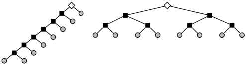
Figure 1: Comparison of tree shapes. Each tree of size eight consists of a root (white diamond), a set of inner nodes (black squares) and a set of leaves (gray circles). The left tree is totally imbalanced, also called comb tree, with depth $d=35/8=4.375$ and Colless index $c=21/21=1$ . The right tree is a complete binary tree with depth $d=24/8=3$ and Colless index $c=0/21=0$ .

The evolutionary history of organisms is represented by a phylogenetic tree. For the purpose of this contribution, a phyologenetic tree is a rooted strict binary tree $T$: a tree with exactly one node (the root) with degree two or zero, all other nodes having degree three (inner node) or one (leaf node), cf. illustrations in Figure 1. For such a tree $T$ with root $w$, a subtree $T^{\prime}$ is obtained as the component not containing $w$ after cutting an edge $\{i,j\}$ of $T$. $T^{\prime}$ is again a rooted strict binary tree. Since this contribution focuses on tree shape, all edges have unit length. The distance between nodes $i$ and $j$ on a tree $T$ is the number of edges contained in the unique path between $i$ and $j$.

From the evolutionary dynamics, an evolving phylogenetic tree $T(t)$ is obtained as follows. At each time step $t$, the leaves of $T(t)$ are the species $S(t)$. When $s$ undergoes specation, two new leaves $s^{\prime}$ and $s^{\prime\prime}$ attach to a leaf $s$. After this event, $s$ is an inner node and no longer a leaf of the tree. In this way, each model of speciation dynamics also defines a model for the growth of a binary tree by iterative splitting of leaves.

2.2 Yule model

In the simplest case, the probability of choosing a species is uniform at each time step, $\pi(s,t)=1/t$. This is the Yule model or ERM model. It serves as a null model of evolution.

The model corresponds to a particularly simple probability distribution on the set of generated trees. For a tree with $n\geq 2$ leaves generated by the Yule model and $i\in\{1,2\dots,n-1\}$, let $p_{\text{ERM}}(i|n)$ be the probability that exactly $i$ leaves are in the left subtree of the root. Then $p_{\text{ERM}}(i|n)=1/(n-1)$. This is shown inductively as follows. Obtaining exactly $i$ leaves at step $n$, either they were already present at the previous step and the speciation took place in the right subtree, or the number increased from $i-1$ to $i$ by speciation in the left subtree. Addition of these products of probabilities for the two cases yields

$$p_{\text{ERM}}(i|n)=\frac{n-1-i}{n-1}p_{\text{ERM}}(i|n-1)+\frac{i-1}{n-1}p_{\text{ERM}}(i-1|n-1)~{}.$$ (2)

With the induction hypothesis $p_{\text{ERM}}(j|n-1)=1/(n-2)$ for all $j$, we obtain

$$p_{\text{ERM}}(i|n)=\frac{(n-1-i)+(i-1)}{(n-1)(n-2)}=\frac{1}{n-1}~{}.$$ (3)

The induction starts with $p_{\text{ERM}}(1|2)=1$ which holds because a tree with two leaves has one leaf each in the left and in the right subtree. Thus the uniform selection of species turns into a uniform distribution on the number of nodes in the left or right subtree. Note that the same distribution applies to each subtree of an ERM tree. Therefore $p_{\text{ERM}}$ fully describes the statistical ensemble of ERM trees. The probability of obtaining a particular tree is the product of $p_{\text{ERM}}$ terms taken over all subtrees. This becomes particularly relevant for modifications of the model taking $p$ non-uniform, see the following subsection.

2.3 Aldous’ branching (AB) model

The class of beta-splitting models defines a distribution of trees by the probability

$$p_{\beta}(i|n)=\frac{1}{\alpha_{\beta}(n)}\frac{\Gamma(\beta+l+1)\Gamma(\beta+n-l+1)}{\Gamma(l+1)\Gamma(n-l+1)}$$ (4)

with appropriate normalization factor $\alpha_{\beta}(n)$. Analogous to $p_{\text{ERM}}$ of the previous subsection, $p_{\beta}(i|n)$ is the probability that a tree has $i$ out of its $n$ leaves in the left subtree. In order to build a tree with $n$ leaves, one first decides according to $p_{\beta}(i|n)$ to have $i$ leaves in the left and $n-i$ leaves in the right subtree. Then the same rule is applied to both subtrees with the determined number of leaves. The recursion into deeper subtrees naturally stops when a subtree is decided to have one leaf.

The parameter $\beta\in[-2;+\infty[$ in Equation (4) tunes the expected imbalance. By increasing $\beta$, equitable splits with $i\approx n/2$ become more probable. The probability distribution of trees from the Yule model is recovered by taking $\beta=0$. The case $\beta=-1.5$ is called Proportional to Distinguishable Arrangements (PDA). It produces a uniform distribution of all ordered (left-right labeled) trees of a given size $n$ [25, 24, 30, 10].

Another interesting case is Aldous’ branching (AB) model [1, 2] obtained for $\beta=-1$, where Equation 4 reads

$$p_{-1}(i|n)\propto\frac{1}{i(n-i)}~{}.$$ (5)

Blum and François have found that $\beta=-1.0$ is the maximum-likelihood choice of $\beta$ over a large set of phylogenetic trees [6]. Therefore we use it as a standard of comparison. The AB model does not have an interpretation in terms of macroevolution, as noted by Blum and François [6]. In particular, it is unknown if its probability distribution of trees can be obtained by stochastic processes of iterated speciation as introduced at the beginning of this section.

2.4 Activity model

In the activity model [15], the set of species $S(t)$ is partitioned into a set of active species $S_{A}(t)$ and a set of inactive species $S_{I}(t)$. At each time step, a species $s\in S_{A}(t)$ is drawn uniformly if $S_{A}(t)$ is non-empty. Otherwise $s\in S_{I}(t)$ is drawn uniformly. The two new species $s^{\prime}$ and $s^{\prime\prime}$ independently enter the active set $S_{A}(t+1)$ with probability $p$. The activation probability $p$ is a parameter of the model. For $p=0.5$ a critical branching process is obtained. Otherwise the model is similar to the Yule model. A variation of the activity model has been introduced by Herrada et al. [16] in the context of protein family trees.

2.5 Age-dependent speciation

In the age model [18], the probability of speciation is inversely proportional to the age of a species. At each time, a species $s\in S(t)$ is drawn with probability

$$\pi_{s}(t)\propto\tau_{s}(t)^{-1}$$ (6)

normalized properly. The age $\tau_{s}$ is the number of time steps passed since creation of species $s$.

2.6 Innovation model

1set $t=1$, $F(0)=\emptyset$, $S(0)=\{\emptyset\}$;

2 while $|S(t)|<N$ do // $N$ as final size of simulated tree

3       if $S(t)\setminus\{s\setminus\{\phi\}:s\in S(t),\phi\in F(t)\}\neq\emptyset$ then

4             // loss event

5             draw $\phi\in F(t)$ uniformly;

6             draw $s\in S(t)$ uniformly;

7             if $s\setminus\{\phi\}\notin S(t)$ then

8                   $S(t+1)=S(t)\cup\{s\setminus\{\phi\}\}$;

9                   $F(t+1)=F(t)$;

10                   increment $t$;

11                  

12            

13      else

14             // innovation event

15             draw $s\in S(t)$ uniformly;

16             set $\phi=1+\max(F(t)\cup\{0\})$;

17             set $S(t+1)=S(t)\cup\{s\cup\{\phi\}\};$

18             set $F(t+1)=F(t)\cup\{\phi\}$;

19             increment $t$;

20            

21      

Algorithm 1 Pseudocode for the innovation model

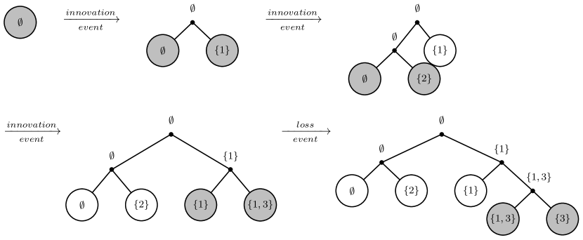
Figure 2: A tree of five leaves generated by the innovation model. The root node labeled with the empty feature set $\emptyset$ speciates by an innovation event adding the feature 1 to the feature set. This results in the species $\emptyset$ and $\{1\}$ . Innovation events are performed, generating features until a loss event is possible. The loss event generates the species $\{3\}$ by removing the feature $1$ from $\{1,3\}$.

In the innovation model, each species $s$ is defined as a finite set of features $s\subseteq\mathbb{N}$. Features are taken as integer numbers in order to have an infinite supply of symbols. We denote by $F(t)$ the set of all features existing at time $t$, that is $F(t)=\bigcup_{s\in S(t)}s$. Each speciation occurs as one of two possible events.

An innovation is the addition of a new feature $\phi\in\mathbb{N}\setminus F(t)$ not yet contained in any species at the given time $t$. One of the resulting species carries the new feature, $s^{\prime}=s\cup\{\phi\}$. The other species has the same features as the ancestral one, $s^{\prime\prime}=s$.

A loss event generates a new species by the disappearance of a feature. A feature $\phi$ is drawn from $F(t)$ uniformly. The loss event is performed only if $s\setminus\{\phi\}\notin S(t)$ such that elimination of $\phi$ from $s$ actually generates a new species. In this case, the resulting species are the one having suffered the loss, $s^{\prime}=s\setminus\{\phi\}$ and the species $s^{\prime\prime}=s$ remaining unaltered. Otherwise, $\phi$ is not present in $s$ or its loss would lead to another already existing species, so nothing happens.

We assume that creation of novel features is significantly less abundant than speciation by losses. This separation of time scales is implemented by the rule that an innovation event is only possible when no more losses can be performed. In order to facilitate further studies with the model, we provide a pseudocode description in Algorithm 1. Figure 2 shows an example of the dynamics.

3 Comparison of simulated and empirical data sets

Figure 3: Empirical and simulated trees. The depicted phylogenetic tree in (a) is from the database TreeBASE (Matrix ID M2957, relationships in rosids based on mitochondrial matR sequences), (b) is a tree created as a realization of the innovation model and (c) a tree from the ERM (Yule) model. Each of the trees has 161 leaves.

Now let us compare the tree shapes obtained by the models with those of evolutionary trees in databases. The TreeBASE [27] database contains phylogenetic information about the evolution of species whereas the database PANDIT [34] contains phylogenetic trees representing protein domains. Analysing the properties with reference to the tree shape of both data sets and applying a comparative study with statistical data sets of different models one can conclude how well a growth model constructs “real” trees.

Comparison by simple inspection of trees from real data and models may already reveal substantial shape differences. Figure 3 shows an example. The trees in panels (a) and (b) are less compact than that of panel (c) of Figure 3.

For an objective and quantitative comparison of trees, we use the following two measures of tree shape. Compactness is best described by the distance $d_{i}$ of a leaf $i$ from root being small. The depth (or Sackin index) [26] is the average distance of leaves from root,

$$d=\frac{\sum_{i=1}^{n}d_{i}}{n}~{}.$$ (7)

The Colless index measures the average imbalance of a tree [9]. The imbalance at an inner node $j$ of the tree is the absolute difference $c_{j}=|l_{j}-r_{j}|$ of leaves in the left and right subtree rooted at $j$. Then the average of imbalances

$$c=\frac{2}{(n-1)(n-2)}\sum_{j=1}^{n-1}c_{j}$$ (8)

with appropriate normalization is the Colless index $c$ of the tree. The index $j$ runs over all $n-1$ inner nodes including the root itself. We find $c=0$ for a totally balanced tree and $c=1$ for a comb tree, see also Figure 1.

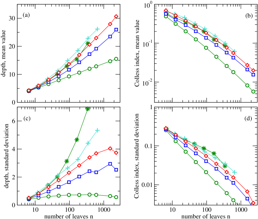
Figure 4: Comparison of size-dependent summary statistics for models and real trees. Symbols distinguish the ERM model ($\circ$), the AB model ($\Box$) and the innovation model ($\diamond$) and the data sets TreeBASE ($\ast$) and PANDIT ($+$). The data sets were preprocessed by solving monotomies and polytomies randomly as well as removing the outgroups as proposed by [6]. The mean values of depth, and Colless index, panels (a) and (b) are binned logarithmically as a function of tree size $n$. The same procedure is applied to the standard deviations, panels (c) and (d). The analysed TreeBASE data set has been downloaded from http://www.treebase.org on June, 2007 containing 5,087 trees of size 5 to 535  after preprocessing. The PANDIT data set has been downloaded from http://www.ebi.ac.uk/goldman-srv/pandit on May 2008 and includes 36,136 preprocessed trees of size 5 to 2,562 . The simulated data set comprises for each model (AB model, ERM model and innovation model) 1,000 trees for each tree size from 5 to 535 and 10 trees for each tree size from 536 to 2,562.

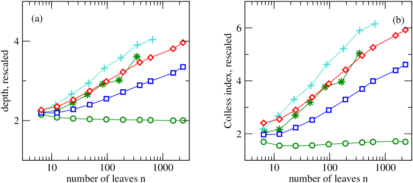
Figure 5: The same values of depth and Colless index as in Figure 4 (a,b) with an $n$-dependent rescaling. (a) Average depth divided by $\ln n$. (b) Average Colless index divided by $n^{-1}\ln n$. These factors are chosen such that the rescaled values for the ERM model asymptotically approach a constant. See refererence [7] for the scaling of the indices of the ERM model.

Ensemble mean values and standard deviations of these indices are shown in Figure 4. Comparing the results of three models (ERM, AB and innovation) to those of trees from two databases, the least discrepancy is obtained between the innovation model and the trees from TreeBASE, representing macroevolution. In Figure 5, the averages of the two indices are shown after rescaling to facilitate the comparison. Of all models, the values of the innovation model are also best matching those of PANDIT.

4 Depth scaling in the innovation model

4.1 Subtree generated by an innovation

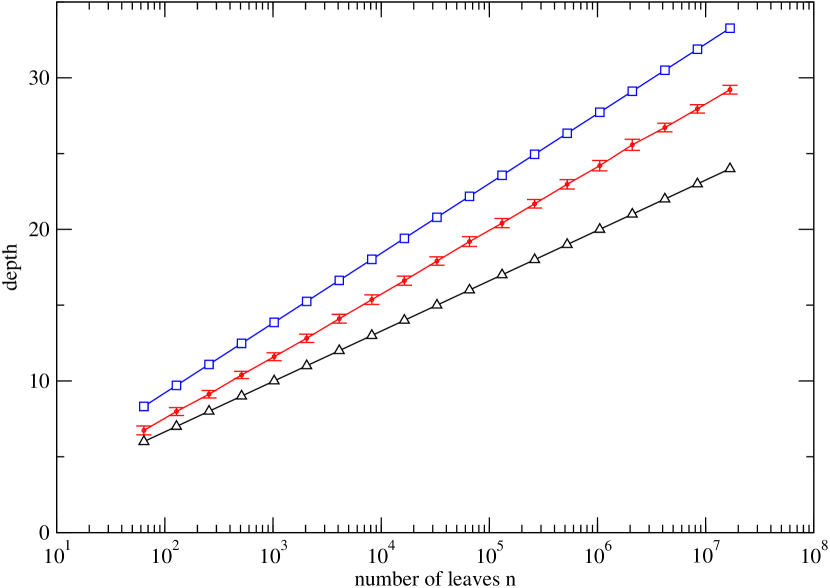
Figure 6: Average depth in dependence of the number of leaves $n$ in trees generated with stochastic loss events (dots with error bars). Each data point is an average over 100 realizations with error bars indicating standard deviations. For comparison, the expected depth for the ERM model ($\Box$) and for complete binary trees ($\triangle$) are shown.

Suppose the $i$-th innovation, generating feature $i$, affects a species $s$ with $f$ features. Then $s$ is removed from the set $S$ of extant species, turning into an inner node in the tree. Two new species $s^{\prime}$ and $s^{\prime\prime}$ are attached, having feature sets $s^{\prime}=s$ and $s^{\prime\prime}=\{i\}\cup s$. In subsequent loss events, a subtree $T_{i}$ is built up with $2^{f}$ leaves, each of which is a species $\sigma\subseteq s\cup\{i\}$. Call $D(T_{i})$ sum of the distances of all the leaves in $T_{i}$ from the root of $T_{i}$.

Let us now estimate the expectation value $\langle D(T_{i})\rangle$, which only depends on the number of features of $f$. Trivially, $D(T_{i})$ is lower bounded by $f2^{f}$ since the most compact tree is the fully balanced one with all nodes at distance $f$ from root. In particular, we conjecture

$$f2^{f}<\langle D(T_{i})\rangle<D_{\text{ERM}}(2^{f})~{}.$$ (9)

The second inequality is corroborated by the plots in Figure 6. We make it plausible as follows. Similar to the ERM model, a leaf is chosen in each time step when executing loss events. Here, however, the loss event is performed only if the chosen leaf carries the chosen feature and the reduced feature set is not yet present in the tree. Thus the probability of accepting a proposed loss event at a leaf $s$ is anticorrelated with the number of features $|s|$ at $s$. The expected number of features carried by a leaf decreases with its distance from root. Therefore we argue that the present model adds new nodes preferentially to leaves closer to root than average, resulting in trees with an expected depth increasing more slowly than in the ERM model.

4.2 Approximation of depth scaling

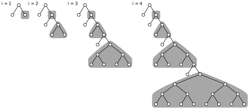
Figure 7: The deterministic growth of a tree considered as an approximation of the innovation model. Each subtree generated by an innovation is indicated as a shaded area.

We study a tree growth that is derived from the innovation model by two simplifying assumptions. (i) Each innovation is introduced at the leaf with the largest number of features in the tree. (ii) Introducing an innovation at a leaf with $f$ features triggers the growth of a subtree that is a perfect (complete) binary tree with $2^{f}$ leaves at distance $f$ from the root of this subtree.

This leads us to consider the following deterministic growth starting with a single node and $i=0$. Choose a leaf $s$ at maximum distance from root; split $s$ obtaining new leaves $s^{\prime}$ and $s^{\prime\prime}$; take $s^{\prime\prime}$ as the root of a newly added subtree that is a perfect tree with $2^{i}$ leaves; increase $i$ by one and iterate. Figure 7 illustrates the first few steps of the growth.

After $i$ steps, the number of leaves added to the tree most recently is $2^{i-1}$. Therefore, the total number of leaves after step $i$ is

$$n(i)=1+\sum_{j=1}^{i}2^{j-1}=2^{i}~{}.$$ (10)

because the procedure starts with a single leaf at $i=0$.

The leaves of the subtree added by the $j$-th innovation have distance

$$\sum_{k=1}^{j}k=\frac{j(j+1)}{2}$$ (11)

from root because these leaves are $j$ levels deeper than those generated by the previous innovation. Therefore the sum of all leaves’ distances from root is

$$D(i)=i+\sum_{j=1}^{n}2^{j-1}[j(j+1)/2]$$ (12)

after the $i$-th innovation has been performed. The first term $i$ arises because the innovation itself renders one previously existing leaf at a distance increased by one, cf. the leaves outside the shaded areas in Figure 7. In performing the sum of Equation 12 we use the equality

$$\sum_{j=0}^{i}x^{j-1}[j(j+1)]=2^{i}[i^{2}-i+2]-2$$ (13)

to arrive at

$$D(i)=i+2^{i-1}[i^{2}-i+2]-1~{}.$$ (14)

We substitute $n(i)=2^{i}$, i.e. $i=\log_{2}n$, and divide $D$ by $n$ to arrive at the depth

$$d(n)=\frac{1}{2}[(\log_{2}n)^{2}-(\log_{2}n)+2]+\frac{(\log_{2}n)-1}{n}$$ (15)

of the tree with $n$ leaves generated by deterministic growth. For large $n$, the depth scaling is

$$d(n)\sim(\log n)^{2}~{}.$$ (16)

By the comparison in Fig. 8, we find the $(\log n)^{2}$ scaling also for the depth of trees obtained from the innovation model as defined in Section 2.6. Thus we hypothesize that the deterministic growth captures the essential mechanism leading to the depth scaling of the innovation model. The prefactor of $(\log n)^{2}$ is smaller in the innovation model than in the deterministic growth. In the actual model, most innovations hit a leaf with a non-maximal number of features and therefore trigger the growth of a lower subtree than assumed by deterministic growth. Table 1 provides an overview of the scaling of average depth with the number of leaves for various tree models .

Table 1: Depth scaling of models.

innovation model	$(\log n)^{2}$
$\beta$-splitting [1]	$\begin{cases}\log n&\text{if }\beta>-1\text{, includes \bf{ ERM} }(\beta=0)\\ (\log n)^{2}&\text{if }\beta=-1\text{, \bf{AB} model}\\ n^{-\beta-1}&\text{if }\beta<-1\text{, includes \bf{ PDA} }(\beta=-1.5)\end{cases}$
age model [18]	$(\log n)^{2}$
activity model [15]	$\begin{cases}n^{0.5}&\text{if }p=0.5,\\ \log n&\text{otherwise.}\end{cases}$
complete tree	$\log n$
comb tree	$n$

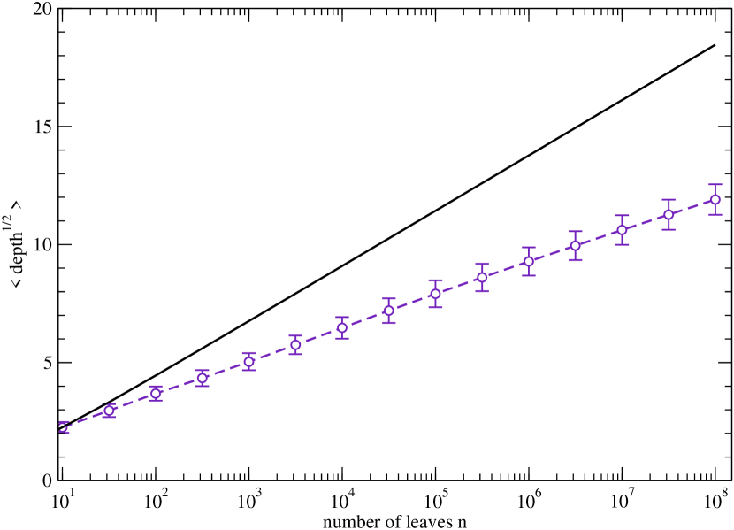
Figure 8: Depth as a function of tree size $n$ for the innovation model ($\circ$) and for the deterministic growth (solid curve) according to Equation (15). Note that square root of depth is plotted such that a straight line in the plot indicates a depth scaling $d(n)\sim(\log n)^{2}$. For each size $n$, the plotted point ($\circ$) is the average over $\sqrt{d(n)}$ for 100 independently generated trees. Error bars give the standard deviation.

5 Discussion

The innovation model establishes a connection between the burstiness of macroevolution and the observed imbalance of phylogenetic trees. Bursts of diversification are triggered by generation of new features and combination with the repertoire of existing traits. In order to keep the model simple, the diversification after an innovation is implemented as a sequence of random losses of features. More realistic versions of the model could be studied where combinations of traits are enriched by re-activation of previously silenced traits or horizontal transfer between species. Furthermore, the model as presented here neglects the extinction of species and their influence on the shapes of phylogenetic trees.

Regarding the robustness of the model, the depth scaling would have to be tested under modifications. In particular, the infinite time scale separation between rare innonvations and frequent loss events could be given up by allowing innovations to occur at a finite rate set as a parameter.

In summary, we have defined a well-working, biologically motivated model which nevertheless is sufficiently simple to allow for further enhancement regarding biological concepts such as sequence evolution and genotype-phenotype relations.

References

- [1] D. Aldous. Probability distributions on cladograms. In D. Aldous and R. Pemantle, editors, Random Discrete Structures, pages 1–18. Springer, 1996.
- [2] D. Aldous. Stochastic models and descriptive statistics for phylogenetic trees, from yule to today. Statistical Science, 16:23–34, 2001.
- [3] R. Axelrod. The Evolution of Cooperation. Basic Books, 1984.
- [4] P. Bak. How Nature Works: The Science of Self-Organised Criticality. Copernicus Press, New York, NY, 1996.
- [5] P. Bak and K. Sneppen. Punctuated equilibrium and criticality in a simple model of evolution. Phys. Rev. Lett., 71:4083–4086, Dec 1993.
- [6] M. G. B. Blum and O. François. Which random processes describe the tree of life? a large-scale study of phylogenetic tree imbalance. Syst. Biol., 55:685–691, 2006.
- [7] M. G. B. Blum, O. François, and S. Janson. The mean, variance and limiting distribution of two statistics sensitive to phylogenetic tree balance. The Annals of Applied Probability, 16(4):2195–2214, 2007.
- [8] P. Campos, V. de Oliveira, and L. Maia. Emergence of allometric scaling in genealogical trees. ADVANCES IN COMPLEX SYSTEMS, 7(1):39–46, 2004.
- [9] D. H. Colless. Phylogenetics: The theory and practice of phylogenetic systematics. Systematic Zoology, 31(1):100–104, 1982.
- [10] J. A. Cotton and R. D. Page. The shape of human gene family phylogenies. BMC Evolutionary Biology, 6:66, 2006.
- [11] C. Darwin. On the Origin of Species. John Murray, 1859.
- [12] S. Gavrilets. Fitness Landscapes and the Origin of Species. Princeton University Press, 2004.
- [13] S. J. Gould and N. Eldredge. Punctuated equilibrium comes of age. Nature, 366:223 – 227, 1993.
- [14] S. B. Heard and D. L. Hauser. Key evolutionary innovations and their ecological mechanisms. Historical Biology, 10(2):151–173, 1995.
- [15] E. Hernández-García, M. Tugrul, A. E. Herrada, V. M. Eguíluz, and K. Klemm. Simple models for scaling in phylogenetic trees. Int. J. Bif. Chaos, 20:805–811, 2010.
- [16] A. Herrada, V. M. Eguíluz, E. Hernández-García, and C. Duarte. Scaling properties of protein family phylogenies. BMC Evolutionary Biology, 11(1):155, 2011.
- [17] A. E. Herrada, C. J. Tessone, K. Klemm, V. M. Eguíluz, E. Hernández-García, and C. M. Duarte. Universal scaling in the branching of the tree of life. PLoS ONE, 3:e2757, 2008.
- [18] S. Keller-Schmidt, M. Tugrul, V. M. Eguíluz, E. Hernández-García, and K. Klemm. An age dependent branching model for macroevolution, 2010.
- [19] M. Kimura. The Neutral Theory of Molecular Evolution. Cambridge University Press, Cambridge, UK, 1983.
- [20] K. Klemm and P. F. Stadler. Rugged and elementary landscapes. In Y. Borenstein, editor, Theory and Principled Methods for Designing Metaheustics. 2012. accepted.
- [21] K. F. Liem and M. H. Nitecki. Key evolutionary innovations, differential diversity, and symecomorphosis, pages 147–170. University of Chicago Press, 1990.
- [22] A. McKenzie and M. Steel. Distributions of cherries for two models of trees. Math. Biosci, 164:81–92, 2000.
- [23] M. Pigliucci. What, if anything, is an evolutionary novelty? Philosophy of Science, 75:887–898, 2008.
- [24] I. Pinelis. Evolutionary models of phylogenetic trees. Proc. R. Soc. Lond. B, 270:1425–1431, 2003.
- [25] D. E. Rosen. Vicariant patterns and historical explanation in biogeography. Systematic Zoology, 27(2):159–188, 1978.
- [26] M. Sackin. Good and bad phenograms. Syst. Zool., 21:225–226, 1972.
- [27] M. J. Sanderson, M. J. Donoghue, W. Piel, and T. Eriksson. TreeBASE: a prototype database of phylogenetic analyses and an interactive tool for browsing the phylogeny of life. American Journal of Botany, 81:183, 1994.
- [28] J. J. Sepkoski. Ten years in the library; new data confirm paleontological patterns. Paleobiology, 19(1):43–51, 1993.
- [29] K. Sneppen, P. Bak, H. Flyvbjerg, and M. H. Jensen. Evolution as a self-organized critical phenomenon. Proceedings of the National Academy of Sciences, 92(11):5209–5213, 1995.
- [30] M. Steel and A. McKenzie. Properties of phylogenetic trees generated by yule-type speciation models. Mathematical Biosciences, 170(1):91–112, 2001.
- [31] Stich, M. and Manrubia, S. C. Topological properties of phylogenetic trees in evolutionary models. European Physical Journal B, 70(4):583–592, 2009.
- [32] K. S. Thomson. Macroevolution: The morphological problem. Society, 32(1):106–112, 1992.
- [33] P. S. Ungar. Mammal teeth: origin, evolution, and diversity. The Johns Hopkins University Press, 2010.
- [34] S. Whelan, P. de Bakker, E. Quevillon, N. Rodriguez, and N. Goldman. Pandit: an evolution-centric database of protein and associated nucleotide domains with inferred trees. Nucleic Acids Res, 2006.
- [35] S. Wright. The roles of mutation, inbreeding, crossbreeeding and selection in evolution. In D. F. Jones, editor, Proceedings of the Sixth International Congress on Genetics, volume 1, pages 356–366, New York, 1932. Brooklyn Botanic Gardens.