Dilaton at the LHC

Abstract

The dilaton, a pseudo-Nambu-Goldstone boson appearing in spontaneous $scale$ $symmetry$ breaking at a TeV scale $f$, may be found in Higgs boson searches. The dilaton couples to standard model fermions and weak bosons with the same structure as the Higgs boson except for the overall strength. Additionally, the dilaton couples to a Higgs boson pair. The couplings of the dilaton to a gluon pair and a photon pair, appearing at loop level, are largely enhanced compared to the corresponding Higgs couplings. We present regions of the mass and VEV of the dilaton allowed by $WW,\ ZZ,$ and $\gamma\gamma$ limits from the LHC at 7 TeV with 1.0-2.3 fb^-1 integrated luminosity. A scale of $f$ less than 1 TeV is nearly excluded. We discuss how the dilaton $\chi$ can be distinguished from the Higgs boson $h^{0}$ by observation of the decays $\chi\rightarrow\gamma\gamma$ and $\chi\rightarrow h^{0}h^{0}\rightarrow(WW)(WW)$.

Discovery of a standard model (SM) Higgs boson $h^{0}$ is a top priority of LHC experiments. However, an experimental signature suggesting the exisitence of a scalar particle does not necessarily mean the discovery of $h^{0}$. There are many candidate theories beyond the SM and almost all predict the existence of new scalar particles. One of these is a dilatonGGS , denoted as $\chi$, which appears as a pseudo-Nambu-Goldstone boson in spontaneous breaking of scale symmetryFujii . The interesting case is that the scale $f$ of conformal symmetry breaking is larger than a weak scale $v$. In this case the dilaton appears as a pseudo-Nambu-Goldstone boson with a mass $m_{\chi}\sim v\ll f$ in addition to the Higgs boson that unitarizes the $WW$ and $ZZ$ scattering amplitudes at the TeV energy scale. This situation occurs in walking technicolor models.Yamawaki ; Bando ; WT1 ; WT2 ; WT3 ; WT4 ; Sannino

It is very important to distinguish the dilaton from $h^{0}$ in observed signals. The dilaton $\chi$ has $T^{\mu}_{\mu}(SM)$ couplings to the SM particles, as will be explained later, which are proportional to the mass for the femions and to mass squared for massive gauge bosons. The couplings are very similar to the SM Higgs $h^{0}$, except that the SM VEV is replaced by $f$. A distinctive difference is in the couplings of massless gauge bosons. The dilaton has a coupling to the trace-anomaly $T^{\mu}_{\mu}(SM)^{\rm anom}$ that is proportional to the $\beta$ function, while the SM Higgs has no such coupling and only triangle-loop diagrams of heavy particles contribute to the $gg$ and $\gamma\gamma$ decays. Because of this property, $h^{0}\rightarrow\gamma\gamma$ is used as a channel searching for the fourth generation and the other heavy exotic particles. While for the dilaton, in the limit of high masses of the heavy particles in the loop, its contribution to the $\beta$ function exactly cancels the triangle diagram of the heavy particles, and thus the dilaton couplings to $gg$ and $\gamma\gamma$ are determined only by $\beta$ function contributions of light-particle loops.

In this Letter we evaluate the production and decays of the dilaton $\chi$ appropriate to the LHC experiments at 7 TeV (LHC7) and consider the possibility that $\chi$ could be found instead of the Higgs boson. We use the dilaton interaction given in Ref.GGS , where the dilaton field $\chi$ is introduced as a compensator for preservation of the non-linear realization of scale symmetry in the effective Lagrangian.

The model parameters are the VEV $f$ of the dilaton and its mass $m_{\chi}$. We derive allowed regions of parameters by considering the latest LHC data relevant to the $WW,ZZ$ and $\gamma\gamma$ decays of the dilaton. The tree-level couplings of $\chi$ to SM particles are very similar to those of $h^{0}$. We consider a possible way to distinguish $\chi$ from $h^{0}$ in two specific decays : $\chi\rightarrow\gamma\gamma$ and $\chi\rightarrow h^{0}h^{0}$.

Dilaton Production Cross-section   The production of the dilaton $\chi$ at a hadron collider is mainly via $gg$ fusion similar to the production of a Higgs boson $h^{0}$. These cross-sections are proportional to the respective partial decay widths to $gg$.

From calculations of Higgs boson production cross-section at NNLODjouadi , we can directly estimate the production cross section of $\chi$ as

$$\sigma(pp\rightarrow\chi X) = \sigma(pp\rightarrow h^{0}X)\times\frac{\Gamma(\chi\rightarrow gg)}{\Gamma(h^{0}\rightarrow gg)}\ .$$ (1)

where we can use the lowest-order results of $\Gamma(\chi\rightarrow gg)$ and $\Gamma(h^{0}\rightarrow gg)$, since in the approximation that the $gg\rightarrow\chi$ interaction is essentially point-like, the QCD radiative corrections to the $gg\rightarrow h^{0}$ and $gg\rightarrow\chi$ subprocesses should be nearly equal. By use of the $\Gamma(\chi\rightarrow gg)$ partial width given later and $\Gamma(h^{0}\rightarrow gg)$ of the SM, we can predict $\sigma(pp\rightarrow\chi X)$. The dilaton result for $f=3$ TeV is compared with the SM Higgs production in Fig. 1.

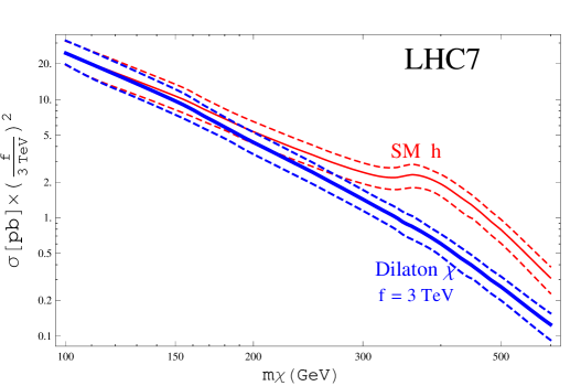
Figure 1: The inclusive dilaton production cross section in pb from $gg$ fusion (solid blue), compared with that of the SM Higgs of the same mass $m_{h^{0}}=m_{\chi}$(solid red). The VEV $f$ of $\chi$ is taken to be 3 TeV. The dilaton production cross-section scales with a factor $(\frac{3~{}{\rm TeV}}{f})^{2}$. The overall theoretical uncertaintiesDjouadi are denoted by the dashed lines.

The production of $\chi$ is almost the same as that of the SM Higgs boson of the same mass $m_{h^{0}}=m_{\chi}$ for the choice $f=3$ TeV used in this figure. The subprocess cross-section $\hat{\sigma}(gg\rightarrow\chi)$ is proportional to $1/f^{2}$. Our prediction of $\sigma(\chi)$ in Fig.1 includes the $\pm 25$% uncertainty associated with the theoretical uncertainty on $\hat{\sigma}(gg\rightarrow h^{0})$.

Dilaton Decay    The dilaton couplings to SM particles are obatinedGGS by using the effective Lagrangian where $\chi$ is introduced as a compensator to preserve a non-linear realization of scale symmetry. The $\chi$ takes a VEV $f$ in the spontaneous scale symmetry breaking and it is redefined by $\chi\rightarrow f+\chi$. In the exact scale symmetric limit, the $\chi$ couples to the SM particles through the trace of the energy-momentum tensor $T_{\mu\nu}(SM)$ as

$$L_{trace} = \frac{\chi}{f}T^{\mu}_{\mu}(SM)\ .$$ (2)

$$T^{\mu}_{\mu}(SM) = T^{\mu}_{\mu}(SM)^{\rm tree}+T^{\mu}_{\mu}(SM)^{\rm anom}$$

$$T^{\mu}_{\mu}(SM)^{\rm tree} = \sum_{f}m_{f}\bar{f}f-2m_{W}^{2}W_{\mu}^{+}W^{-\ \mu}-m_{Z}^{2}Z_{\mu}Z^{\mu}+2m_{h}^{2}h^{2}-\partial_{\mu}h\partial^{\mu}h$$

$$T_{\mu}^{\mu}(SM)^{\rm anom} = -\frac{\alpha_{s}}{8\pi}b_{QCD}\sum_{a}F^{a}_{\mu\nu}F^{a\mu\nu}-\frac{\alpha}{8\pi}b_{EM}F_{\mu\nu}F^{\mu\nu}\ \ .$$ (3)

Here $T^{\mu}_{\mu}(SM)$, the trace of the SM energy-momentum tensor, defined by $\sqrt{-g}T_{\mu\nu}(SM)=2\frac{\delta(\sqrt{-g}L_{SM})}{\delta g^{\mu\nu}}$, is represented as a sum of the tree-level term $T^{\mu}_{\mu}(SM)^{\rm tree}$ and the trace anomaly term $T_{\mu}^{\mu}(SM)^{\rm anom}$ for gluons and photons, where $F^{a}_{\mu\nu}(F_{\mu\nu})$ are the respective field strengths. The $T^{\mu}_{\mu}(SM)^{\rm tree}$ contributions are proportional to the fermion masses and the squares of weak boson masses.

The $b$ values of the $\beta$ functions are

$$b_{QCD} = 11-(2/3)6+F_{t}\ \ \ {\rm and}\ \ \ b_{EM}=19/6-41/6+(8/3)F_{t}-F_{W}$$ (4)

which include the QCD top triangle-loop and the top and $W$ EM triangle-loops. The triangle functions are given by

$$F_{t} = \tau_{t}(1+(1-\tau_{t})f(\tau_{t})),\ \ \ F_{W}=2+3\tau_{W}+3\tau_{W}(2-\tau_{W})f(\tau_{W})$$ (8)

$$f(\tau)=\left\{\begin{array}[]{lc}[{\rm Arcsin}\frac{1}{\sqrt{\tau}}]^{2}&{\rm for}\ \tau\geq 1\\ -\frac{1}{4}[{\rm ln}\frac{\eta_{+}}{\eta_{-}}-i\pi]^{2}&{\rm for}\ \tau<1\end{array}\right.$$

$$\eta_{\pm}=1\pm\sqrt{1-\tau},\ \ \ \tau_{i}\equiv\left(\frac{2m_{i}}{m_{\phi}}\right)^{2}\ {\rm for}\ i=t,W.$$

The dilaton couplings are very similar to those of the SM Higgs except that there is a distinctive difference in the $gg$ and $\gamma\gamma$ couplings. For the dilaton $\chi$, $b_{QCD,EM}$ in Eq. (4) are given by

$$b_{QCD}^{\chi}\simeq\left\{\begin{array}[]{cr}11-\frac{2}{3}5&\ \ \ m_{\chi}<2m_{t}\\ 11-\frac{2}{3}6&2m_{t}<m_{\chi}\end{array}\right. ,\ \ \ b_{EM}^{\chi}\simeq\left\{\begin{array}[]{cr}-\frac{80}{9}&m_{\chi}<2m_{W}\\ -\frac{35}{9}&\ \ \ 2m_{W}<m_{\chi}<2m_{t}\\ -\frac{17}{3}&2m_{t}<m_{\chi}\end{array}\right.\ .$$ (14)

Here $b_{QCD}$ for $m_{\chi}<2m_{t}$ is represented as $11-\frac{2}{3}n_{\rm light}$ with the number of light flavors $n_{\rm light}=5$ as explained above. For the case of the SM Higgs $h^{0}$, the corresponding $b$ values are

$$b_{QCD}^{h^{0}}=F_{t}\simeq\left\{\begin{array}[]{cr}\frac{2}{3}&m_{h}<2m_{t}\\ 0&\ \ \ 2m_{t}<m_{h}\end{array}\right. ,\ \ \ b_{EM}^{h^{0}}=\frac{8}{3}F_{t}-F_{W}\simeq\left\{\begin{array}[]{cr}-\frac{47}{9}&m_{h}<2m_{W}\\ \frac{-2}{9}&\ \ \ 2m_{W}<m_{h}<2m_{t}\\ -2&2m_{t}<m_{h}\end{array}\right.\ .\ \ \$$ (20)

There is a strong enhancement of $gg$ and $\gamma\gamma$ couplings of $\chi$ compared to the $h^{0}$, as previously discussed in ref.GGS .

Another important dilaton decay channel is $h^{0}h^{0}$. Models with $f>v$ predict the scalar unitarizing $WW,ZZ$ scattering amplitudes to have mass in the TeV region, but there is no compelling reason to forbid the situation $m_{h}<m_{\chi}/2$. Observing $\chi\rightarrow h^{0}h^{0}\rightarrow(WW)(WW),\ (WW)(ZZ),$ or $(ZZ)(ZZ)$ is a decisive way to distinguish $\chi$ from $h^{0}$.

The kinetic and mass terms of $\chi$ are givenGGS by

$${\cal L}_{\chi} = \frac{1}{2}\partial_{\mu}{\chi}\partial^{\mu}{\chi}-\frac{m_{\chi}^{2}}{2}\chi^{2}-\frac{m_{\chi}^{2}}{2f}\chi^{3}+\cdots.$$ (21)

where we consider an explicit scale symmetry breaking parameter with dimension 2 by having a Higgs mass term in the SM. This ${\cal L}_{\chi}$ duplicates the SM Higgs interactions when $f$ is replaced by $v$.

For the $\chi$ decay channels $\chi\rightarrow AB$, we consider $AB=gg,\gamma\gamma$,$W^{+}W^{-}$, $ZZ,b\bar{b},t\bar{t},c\bar{c},\tau^{+}\tau^{-}$, and $h^{0}h^{0}$. The decay branching fractions of $\chi$ are given in Fig. 2. The QCD radiative correction in NNLOKfact comment2 is taken into account for the gg channel. The QCD radiative corrections to $b\bar{b},c\bar{c}$ and $t\bar{t}$ at NLO are included. The off-shell $WW^{*}$ and $ZZ^{*}$ decays are treated as in ref.Keung .

A large $gg$ branching fraction at $m_{\chi}\stackrel{{\scriptstyle<}}{{\scriptscriptstyle\sim}}140$ GeV is a characteristic of $\chi$ decay in comparison with $h^{0}$ decays where $h^{0}\rightarrow b\bar{b}$ is the dominant channel for $m_{h^{0}}\stackrel{{\scriptstyle<}}{{\scriptscriptstyle\sim}}140$ GeV, as pointed out in ref.GGS .

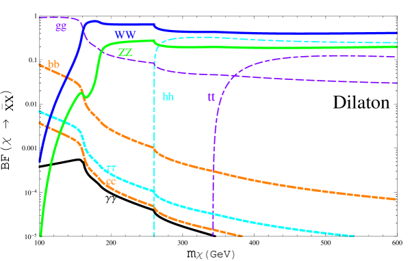
Figure 2: Decay Branching Fractions of $\chi$ versus $m_{\chi}$(GeV). $m_{h^{0}}$ is taken to be 130 GeV. The result is independent of the value of $f$.

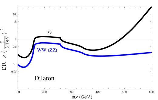
Figure 3: $\chi$ Detection Ratio ($DR$) to the SM higgs $h^{0}$ of Eq. (21) for the $\bar{X}X=W^{+}W^{-}$(solid blue) and $\gamma\gamma$ (solid black) final states versus $m_{\chi}$(GeV). Note that $DR(ZZ)=DR(WW)$. $f$ is taken to be 3 TeV. $DR$ scales with a factor $(\frac{3~{}{\rm TeV}}{f})^{2}$.

Dilaton Detection compared to SM Higgs     Next we consider the detection of $\chi$ in the $W^{+}W^{-}$, $ZZ$ and $\gamma\gamma$ channels. The $\chi$ detection ratio ($DR$) to $h^{0}$ in the $\bar{X}X$ channel is definedbook by

$$DR \equiv \frac{\displaystyle\Gamma_{\chi\rightarrow gg}\Gamma_{\chi\rightarrow\bar{X}X}/\Gamma_{\chi}^{\rm tot}}{\displaystyle\Gamma_{h^{0}\rightarrow gg}\Gamma_{h^{0}\rightarrow\bar{X}X}/\Gamma_{h^{0}}^{\rm tot}}\ ,\ \ \ \ \ \ \ \ \$$ (22)

where $\bar{X}X=W^{+}W^{-},\ ZZ,$ and $\gamma\gamma$. The $DR$ are plotted versus $m_{\chi}=m_{h^{0}}$ in Fig. 3 for $f=3$ TeV.

$DR(WW)=DR(ZZ)$ in all mass regions. $DR$ of the $WW,\ ZZ,$ and $\gamma\gamma$ are all relatively large in the mass range $160<m_{\chi}<260$ GeV, between the WW threshold and the $h^{0}h^{0}$ threshold. $DR(\gamma\gamma)$ is larger than those of $WW,ZZ$ in all mass regions because of the enhancement evident in Eq. (14).

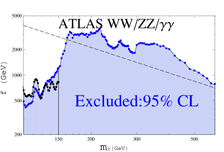
Figure 4: The allowed regions of dilaton parameters $(f,m_{\chi})$ in GeV at the 95% confidence level, determined from ATLAS data. We use $DR(WW)$ for the ATLASAtlas combined result (blue points and solid line), which are obtained from the results for $H\rightarrow WW\rightarrow l\nu l\nu$ (1.70 fb^-1), $H\rightarrow ZZ\rightarrow llll$ (1.96-2.28 fb^-1), $H\rightarrow ZZ\rightarrow llqq$ (1.04 fb^-1), and $H\rightarrow ZZ\rightarrow ll\nu\nu$ (1.04 fb^-1) at $m_{H}>150$GeV. At $m_{\chi}<150$ GeV, the constraint from $\gamma\gamma$ data with 1.08 fb^-1 (black points and solid lines), improves on the $WW/ZZ$ constraints. See, also related previousBai and subsequentLogan ; John works. The dashed line represents a prediction of a walking technicolor model, $f\simeq\frac{1413}{2}(\frac{600GeV}{m_{\chi}})$GeVYamawaki2 in a partially gauged one-doublet modelChris ; Luty with $(N_{TC},N_{TF})=(2,8)$ or $(3,12)$.

The cross-section of a putative Higgs-boson signal, relative to the Standard Model cross section, as a function of the assumed Higgs boson mass, is widely used by the experimental groups to determine the allowed and excluded regions of $m_{h^{0}}$. By use of the $DR$ in Fig. 3, we can determine the allowed regions of $f$ and $m_{\chi}$. First we consider the quantity $(1/DR)\times(\sigma_{\rm exp}/\sigma(h^{0}\rightarrow\bar{X}X))$. This is the signal of the Higgs boson decaying into $\bar{X}X$ relative to the dilaton cross section $[\sigma(\chi\rightarrow\bar{X}X)=\sigma(h^{0}\rightarrow\bar{X}X)\times DR]$ for $\bar{X}X=WW,ZZ,\gamma\gamma$. $DR$ is proportional to $(1/f)^{2}$. The $f$ corresponding to the 95% CL upper limit of $\sigma_{\rm exp}$ gives the lower limit on the allowed region of $f$. The ATLAS exclusion of $h^{0}$ is obtained by combining $WW$ and $ZZ$ data for $m_{h^{0}}>150$ GeV, and including $\gamma\gamma$ for $m_{h^{0}}<150$ GeV. We can use the $DR(WW)$ for the ATLAS combined result since the model prediction is $DR(WW)=DR(ZZ)<DR(\gamma\gamma)$ which is valid in all mass regions, as can be seen in Fig. 3. The figure 4 shows the exclusion regions of dilaton parameters at 95% confidence level.

The $\gamma\gamma$ final state is very promising for $\chi$ detection, because the $\chi$ detection ratio to $h^{0}$ is generally very large in all the mass range of $m_{\chi}$, as is evident in Fig. 3. For $m_{\chi}>150$ GeV, the detection of a $\gamma\gamma$ signal can be a key to distinguish $\chi$ and $h^{0}$, although the $\gamma\gamma$ BF of $\chi$ is itself small.

Concluding Remarks    We have investigated a search for the dilaton $\chi$ at LHC7. The VEV $f<1$ TeV is not favorable, but large allowed regions of $f$ and $m_{\chi}$ are consistent with the present data. The forthcoming 5 fb^-1 integrated luminosity at LHC7 will substantially extend the discovery or exclusion regions. The coupling of $\chi$ is very similar to the $h^{0}$; however, it is posssible to distinguish it from the SM $h^{0}$ by observing the $\gamma\gamma$ decay rate relative to $WW$. The $\chi\rightarrow h^{0}h^{0}$ decay is a distinguishing feature of the dilaton from the SM Higgs, It will give $(WW)(WW),\ (WW)(ZZ),$ and $(ZZ)(ZZ)$ final states, which have low backgrounds.

If the LHC7 finds no signal of a scalar in forthcoming 5 fb^-1 data, we still have a possibility of a low-mass dilaton with $f>3$ TeV. In this case the walking techincolor modelYamawaki ; Bando ; WT1 ; WT2 ; WT3 ; WT4 ; Sannino are promising wherein the Higgs scalar unitarizing the $WW,ZZ$ scattering amplitudes appears in the TeV region.

Acknowledgements

M.I. is very grateful to the members of phenomenology institute of University of Wisconsin-Madison for hospitalities. This work was supported in part by the U.S. Department of Energy under grants No. DE-FG02-95ER40896 and DE-FG02-84ER40173, in part by KAKENHI(2274015, Grant-in-Aid for Young Scientists(B)) and in part by grant as Special Researcher of Meisei University.

References

(1) W. D. Goldberger, B. Grinstein, and W. Skiba, Phys. Rev. Lett. 100, 111802 (2008).
(2) ”Gravitation and scalar fields,” Y. Fujii, Kodansha scientific 1997 (in Japanese).
(3) K. Yamawaki, M. Bando and K. -i. Matumoto,
Phys. Rev. Lett. 56, 1335 (1986).
(4) M. Bando, K. -i. Matumoto and K. Yamawaki,
Phys. Lett. B 178, 308 (1986).
(5) B. Holdom, Phys. Lett. B150, 301 (1985).
(6) T. W. Appelquist, D. Karabali, and L. C. R. Wijewardhana, Phys. Rev. Lett. 57, 957 (1986).
(7) M. A. Luty, T. Okui, JHEP 0609, 070 (2006).
(8) R. Rattazzi, V. S. Rychkov, E. Tonni, A. Vichi, JHEP 0812, 031 (2008).
(9) D. D. Dietrich, and F. Sannino, Phys. Rev. D72, 055001 (2005).
(10) J. Baglio and A. Djouadi, arXiv:1012.0530v3 [hep-ph]; JHEP03, 055 (2011).
(11) S. Catani, D. de Florian, M. Grazzini, and P. Nason, JHEP07, 028 (2003).
(12) We use central values of K-factor of Higgs production in NNLO given in Fig. 8 of
Ref.Kfact: For GeV, .
This value is about 10% larger than the K-factor of Higgs decaying into in NNLO given in ref.decayK
but within the uncertainty of the choice of the renormalization scale. We assume they are equal and adopt the
value in ref.Kfact.
(13) M. Schreck and M. Steinhauser, arXiv:0708:0916v2 [hep-ph]; Phys. Lett. B655, 148 (2007).
(14) W.-Y. Keung and W. J. Marciano, Phys. Rev. D30, 248 (1984).
(15) V. D. Barger and R. J. N. Phillips, ”Collider Physics” Updated Edition, Westview press,
Boulder, Colorado (1991).
(16) The ATLAS Collaboration, ATLAS-CONF-2011-135, Sep. 30, 2011.
(17) Y. Bai, M. Carena, and J. Lykken, arXiv: 0909.1319v2 [hep-ph];
Phys. Rev. Lett. 103, 261803 (2009).
(18) B. Coleppa, T. Gregoire, and H. E. Logan, arXiv:1111.3276v1[hep-ph].
(19) B. A. Campbell, J. Ellis, and K. A. Olive, arXiv:1111.4495[hep-ph].
(20)S. Matsuzaki and K. Yamawaki,
arXiv:1109.5448 [hep-ph].
(21) N. D. Christensen and R. Schrock, Phys. Lett. B632, 92(2006).