Entanglement of distant optomechanical systems

Abstract

We theoretically investigate the possibility to generate non-classical states of optical and mechanical modes of optical cavities, distant from each other. A setup comprised of two identical cavities, each with one fixed and one movable mirror and coupled by an optical fiber, is studied in detail. We show that with such a setup there is potential to generate entanglement between the distant cavities, involving both optical and mechanical modes. The scheme is robust with respect to dissipation, and nonlocal correlations are found to exist in the steady state at finite temperatures.

I Introduction

Quantum entanglement is one of the most intriguing features of quantum mechanics. Although quantum mechanics has proven to be highly successful in explaining physics at microscopic and subatomic scales, its validity at macroscopic or even mesoscopic scales is still debated. Some of the astonishing features appear when we try to apply quantum mechanical principles to macroscopic systems. Superpositions of macroscopic systems is one example schr .

It is not yet completely clear to what extent quantum mechanics applies to macroscopic objects. Quantum phenomena such as entanglement generally do not appear in the macroscopic world. The difficulty of seeing quantum superpositions of macroscopic systems is often attributed to environment-induced decoherence. Such decoherence is thought to be the main cause reducing any quantum superposition to a classical statistical mixture zure . Thus, an obvious but impractical choice would be to minimize the detrimental effect of the environment through perfect isolation of the system of interest. Nonetheless, with the spectacular level of experimental advancements, the possibility of seeing macroscopic quantum superpositions appears to be within reach c60 .

Related to this, quantum engineering qcon in the field of optomechanics has made rapid advancement flor . In a typical optomechanical setup, a mechanical system can be manipulated by radiation forces. Such systems have recently attracted much theoretical and experimental attention tjki ; tjki2 . This is partly because of their potential usefulness in extremely sensitive sensor technology and in quantum information processing tjki . Also, they are potentially one of the best tools to test fundamentals of quantum mechanics. Seminal progress has been made both theoretically and experimentally in this novel emerging field flor ; tjki2 .

In a typical setting using optomechanical interaction, the main component is a cavity with a movable mirror. Light in the cavity and the movable mirror interact due to a coupling induced by the radiation pressure. As a result, the movable mirror executes harmonic motion around its equilibrium value lasing , which thus alters the cavity resonance frequency. This, in turn, changes the circulating power in the cavity and hence the radiation pressure force acting on the movable mirror, leading to intrinsic nonlinearities walther . Strong light-matter coupling, both for opto- and for electro-mechanical systems, is a main ingredient in this emerging research field simo ; teuf . Within the strong coupling regime, radiation-pressure interaction has been successfully utilized for ground state cooling of mechanical oscillators iwra ; simo3 ; connell . Some of the fascinating schemes include preparing the cavity mode and the movable mirror in a non-classical state smans ; sbos , preparing optomechanical or fully mechanical Schrödinger cat states  smans3 ; agarwal ; laura , and even inducing quantum correlations between the subsystems shbar ; mment ; mfent ; mment2 . Apart from the mostly studied cavity-movable mirror geometry, there have been some recent breakthroughs in exploring quantum features of a membrane in a cavity jdthom ; bhatta . There are also recent proposals exploring the possibility of observing photonic analogs of the Josephson effect in an optomechanical setting larson .

A common feature of most of these studies involve enhancement of the radiation pressure coupling through intense laser driving of the cavity field. This is required to achieve strong radiation pressure coupling which otherwise is too weak to observe any non-classical phenomenon. Although most of these studies are restricted to Gaussian state preparation involving optomechanical interaction, there have been some recent proposals to study non-Gaussian quantum states in the regime of single-photon optomechanics akram ; anunn .

Motivated by these theoretical and experimental advancements, we shall here explore the possibility of entangling mechanical and optical modes of two distant cavities. In previous studies of the entanglement of distant mechanical mirrors, squeezed light was used as an available resource in order to entangle the two distant mirrors, which were either part of the same optical cavity agarwal ; mment or belonged to two different cavities laura . In the present work we are interested in a physically different setup, where two distant Fabry-Pérot cavities each fabricated with one movable mirror are coupled by an optical fiber. We show that, as a result of a combination of the optomechanical interaction and an optical-fiber mediated coupling, the two distant optical and mechanical modes become entangled. Moreover, we explicitly study two different regimes of physical interest. First we will impose an approximation of Born-Oppenheimer (BO) type, and consider a scenario in which the two cavities are not externally pumped. In this regime the two mechanical modes are found not to be very strongly entangled. The advantage is however that the approximation allows us to find an analytical solution describing the evolution of the state of the two mirrors. Thereafter we work in a regime where the coupled cavities are strongly driven. Here we explicitly derive the relevant quantum Langevin equations (QLE) and construct the covariance matrix governing the dynamics of all the optical and mechanical modes.

The paper is organized in the following way. Section II introduces the theoretical model and the physical setup. This forms the framework for Sec. III.2 in which the unitary evolution of the system is studied, followed by analysis of the dissipative regime in Sec. III.3 and a brief discussion on the validity of the BO approximation in Sec. III.4. A quantum Langevin approach is introduced in Sec. IV, and we conclude with a short discussion in Sec. V.

II Physical setup

We consider a physical setup comprised of two identical Fabry-Pérot cavities, each with one fixed and one movable mirror, as schematically shown in Fig. 1. We assume that only one resonant mode of each cavity is populated, and that these two modes are coupled via an optical fiber. The two modes have the same frequency, $\omega=2\pi c/L$; where $L$ is the cavity length, and are described by the creation (annihilation) operators $\hat{a}^{\dagger}(\hat{a})$ and $\hat{b}^{\dagger}(\hat{b})$, respectively. Furthermore, we assume that each movable mirror has been cooled near to its ground state, so that it is operating in the quantum regime. Under the action of cavity-photon-induced radiation pressure, the movable mirrors will oscillate about their equilibrium positions.

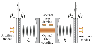
Figure 1: (Color online) Sketch of the physical setup to entangle distant optomechanical modes. Two optomechanical cavities pumped by classical laser fields are coupled to each other by an optical fibre. As a result of indirect coupling mediated by the two cavity modes, the two movable mirrors become entangled. Furthermore, two initially uncorrelated auxiliary cavity modes interact independently with the two entangled movable mirrors, which induces non-local correlations between the two modes. Using standard homodyne measurement techniques non-local correlations between the two auxiliary cavity modes can be read out giving an indirect signature of quantum correlations between the two mirrors.

If we assume that the two mirrors move distances $x$ and $y$ along the respective cavity axes, so that the two displacements are much smaller than the wavelength of each cavity mode in one cavity round-trip time, then scattering of photons to other cavity modes can be safely neglected afpa ; law . The effective lengths of the cavities will then become $L+x$ and $L+y$, with new resonance frequencies $\omega_{a}=2\pi c/(L+x)$ and $\omega_{b}=2\pi c/(L+y)$, where $x$ and $y$ are the instantaneous displacements of the two cavity mirrors from their equilibrium positions. With the above assumption, i.e. $x/L,y/L\ll 1$, the free evolution of the two optical cavity modes in the adiabatic regime takes the form law

$$\hat{H}_{\rm free} = \hbar\omega_{a}\hat{a}^{\dagger}\hat{a}+\hbar\omega_{b}\hat{b}^{\dagger}\hat{b}$$

$$= \hbar\omega\left(1+\frac{x}{L}\right)^{-1}\hat{a}^{\dagger}\hat{a}+\hbar\omega\left(1+\frac{y}{L}\right)^{-1}\hat{b}^{\dagger}\hat{b}$$

$$\approx \hbar\omega\left(\hat{a}^{\dagger}\hat{a}+\hat{b}^{\dagger}\hat{b}\right)-\frac{\hbar\omega}{L}\hat{a}^{\dagger}\hat{a}x-\frac{\hbar\omega}{L}\hat{b}^{\dagger}\hat{b}y.$$

Under the action of a weak radiation-pressure force, each movable mirror undergoes small-amplitude oscillations with frequency $\Omega$. In the absence of external driving, the full Hamiltonian of the two coupled cavities thus becomes

$$\hat{H}=\hat{H}_{\rm free}+\frac{m\Omega^{2}}{2}x^{2}+\frac{p_{x}^{2}}{2m}+\frac{m\Omega^{2}}{2}y^{2}+\frac{p_{y}^{2}}{2m}+\hbar\lambda\left(\hat{a}^{\dagger}\hat{b}+\hat{b}^{\dagger}\hat{a}\right),$$ (2)

where $\lambda$ is the inter-mode coupling between the two cavities. This coupling could be mediated by, e.g., an optical fiber connecting the two distant cavities. Introducing dimensionless conjugate variables $q_{i}$ and $p_{i}$ for the $i$th movable mirror, (2) can be rewritten as

$$\hat{H} = {\hbar}{\omega\left(\hat{a}^{\dagger}\hat{a}+\hat{b}^{\dagger}\hat{b}\right)+\frac{\hbar\Omega}{2}\left(\hat{q_{1}}^{2}+\hat{p_{1}}^{2}\right)+\frac{\hbar\Omega}{2}\left(\hat{q_{2}}^{2}+\hat{p_{2}}^{2}\right)}$$ (3)

$$+\hbar\lambda\left(\hat{a}^{\dagger}\hat{b}+\hat{b}^{\dagger}\hat{a}\right)-\hbar g\left(\hat{a}^{\dagger}\hat{a}\hat{q_{1}}+\hat{b}^{\dagger}\hat{b}\hat{q_{2}}\right),$$

where $g=(\omega/L)\sqrt{\hbar/m\Omega}$ is the radiation pressure-induced coupling between the cavity modes and the movable mirrors. The Hamiltonian (3) will form the basis for the analysis in the next section, where we will make an adiabatic approximation that allows us to study the unitary evolution of the two movable mirrors.

III Born-Oppenheimer approach

III.1 Effective adiabatic model

The frequency mismatch between optical ($\omega/2\pi\sim 10^{14}$ Hz) and mechanical ($\Omega/2\pi\sim 10^{6}-10^{9}$ Hz) degrees of freedom is enormous tjki2 . This suggests a separation of the Hamiltonian (3) into two parts, one with very rapidly evolving optical modes and another with slowly varying mechanical modes. In the limit that the mirror coordinates $\hat{q}_{1}$ and $\hat{q}_{2}$ remain stationary with respect to the rapidly evolving cavity modes $\hat{a}$ and $\hat{b}$, we can diagonalize the interaction between the two cavity modes of Hamiltonian (3).

We first introduce the collective excitation operators $\hat{A}$ and $\hat{B}$ obeying

$$\left(\begin{array}[]{c}\hat{a}\\ \hat{b}\end{array}\right)=\left(\begin{array}[]{cc}\rm{cos}\theta&\rm{sin}\theta\\ -\rm{sin}\theta&\rm{cos}\theta\end{array}\right)\left(\begin{array}[]{c}\hat{A}\\ \hat{B}\end{array}\right).$$ (4)

Choosing $\tan 2\theta=2\lambda/(g(q_{1}-q_{2}))$ and substituting for the new field modes, the rapidly varying optical part of Hamiltonian (3) reduces to

$$\hat{H}_{\rm{cav}} = \hbar\left(\omega-g\frac{q_{1}+q_{2}}{2}\right)(\hat{A}^{\dagger}\hat{A}+\hat{B}^{\dagger}\hat{B})$$ (5)

$$-\hbar\sqrt{g^{2}{\left(q_{1}-q_{2}\right)^{2}+4\lambda^{2}}}\frac{(\hat{A}^{\dagger}\hat{A}-\hat{B}^{\dagger}\hat{B})}{2}.$$

The Hamiltonian describing the dynamics of the two movable cavity mirrors thus takes the form

$$\hat{H}_{\rm{mir}}=\hbar\frac{\Omega}{2}\left(\hat{q_{1}}^{2}+\hat{p_{1}}^{2}+\hat{q_{2}}^{2}+\hat{p_{2}}^{2}\right)+\hat{H}_{\rm{cav}}.$$ (6)

The treatment this far is exact. Typically, the cavity field will adiabatically follow the slow motion of the two movable mirrors. Thus by considering rapidly varying collective cavity modes and slowly varying mirror modes we can make the BO approximation BO ; lsced , and write the collective wave function of the cavity-mirror coupled system at time $t$ as

$$|\Psi(t)\rangle=\sum_{n_{A},n_{B}}P(n_{A},n_{B})|n\rangle|\Phi(n,t)\rangle.$$ (7)

Here, $P(n_{A},n_{B})$ is the probability distribution of the collective cavity fields, $|n\rangle$=$|n_{A},n_{B}\rangle$ denotes the time-independent index of the energy levels of the two collective cavity modes $\hat{A}$ and $\hat{B}$, in the adiabatic limit, in which $\hat{A}^{\dagger}\hat{A}|n\rangle=n_{A}|n\rangle$ and $\hat{B}^{\dagger}\hat{B}|n\rangle=n_{B}|n\rangle$, and $|\Phi(n,t)\rangle=e^{-i\hat{H}_{\rm{mir}}t/\hbar}|\Phi(n,0)\rangle$ denotes the time-evolved wave function of the two movable mirrors cpsun ; hian . The approximation in assigning a system wave function of the form (7) lies in the fact that the coefficients $P(n_{A},n_{B})$ are time-independent, and as a consequence no population transfer occurs between different photon states $|n\rangle$.

Within this BO approximation, the cavity modes can be seen as inducing an effective potential in which the two mirrors evolve,

$$\hat{V}_{\rm{eff}} = \hbar\left(\omega-g\frac{q_{1}+q_{2}}{2}\right)(n_{A}+n_{B})$$ (8)

$$-\hbar\sqrt{g^{2}(q_{1}-q_{2})^{2}+4\lambda^{2}}\frac{n_{A}-n_{B}}{2}.$$

Since we have assumed that the oscillation amplitudes of the movable mirrors are small, it follows that their relative displacement $\hat{q}_{1}-\hat{q}_{2}$ is also small. Therefore, it is sufficient to expand the second term in the cavity Hamiltonian (8) to second (quadratic) order in $\hat{q}_{1}-\hat{q}_{2}$. This can be justified, since for a typical optomechanical cavity with optical frequency $\omega/2\pi\sim 10^{14}~{}{\rm Hz}$, length $L\sim 1~{}{\rm mm}$, mirror frequency $\Omega/2\pi\sim 10^{6}~{}{\rm Hz}$, and with a zero-point-oscillation amplitude of $0.02~{}{\rm pm}$, one finds that $g\sim 10^{4}~{}{\rm Hz}$. With the reasonable estimate $\lambda=10^{5}~{}{\rm Hz}$ one gets $(g/2\lambda)^{2}\sim 10^{-3}$. This results in an effective Hamiltonian describing the dynamics of two coupled movable mirror in absence of any losses,

$$\hat{H}_{\rm{mir}}\approx\hbar\frac{\Omega}{2}\left(\hat{q_{1}}^{2}+\hat{p_{1}}^{2}+\hat{q_{2}}^{2}+\hat{p_{2}}^{2}\right)$$ (9)

$$-(n_{A}-n_{B})\hbar\lambda\frac{g^{2}}{8\lambda^{2}}(\hat{q_{1}}-\hat{q_{2}})^{2},$$

where we have dropped all the constant and classical driving terms from the Hamiltonian. Dynamical properties of entanglement in a model related to the one of Eq. (9) was recently studied for a closed system fernanda . Equation (6) can be rewritten in terms of

$$\hat{q}_{1}=\frac{(\hat{c}^{\dagger}+\hat{c})}{\sqrt{2}},~{}~{}~{}~{}~{}~{}\hat{p}_{1}=i\frac{(\hat{c}^{\dagger}-\hat{c})}{\sqrt{2}},$$

$$\hat{q}_{2}=\frac{(\hat{d}^{\dagger}+\hat{d})}{\sqrt{2}},~{}~{}~{}~{}~{}~{}\hat{p}_{2}=i\frac{(\hat{d}^{\dagger}-\hat{d})}{\sqrt{2}},$$

such that

$$\hat{H}_{\rm{mir}} = \hbar\Omega\left(\hat{c}^{\dagger}\hat{c}+\hat{d}^{\dagger}\hat{d}\right)$$

$$-(n_{A}-n_{B})\hbar\lambda\left(\frac{g^{2}}{16\lambda^{2}}\right)\left(\hat{c}^{2}+\hat{c}^{\dagger 2}+2\hat{c}^{\dagger}\hat{c}\right)$$

$$-(n_{A}-n_{B})\hbar\lambda\left(\frac{g^{2}}{16\lambda^{2}}\right)\left(\hat{d}^{2}+\hat{d}^{\dagger 2}+2\hat{d}^{\dagger}\hat{d}\right)$$

$$+(n_{A}-n_{B})\hbar\lambda\left(\frac{g^{2}}{8\lambda^{2}}\right)\left(\hat{c}+\hat{c}^{\dagger}\right)\left(\hat{d}+\hat{d}^{\dagger}\right).$$

Introducing center-of-mass and relative modes,

$$\hat{C}=\frac{\hat{c}+\hat{d}}{\sqrt{2}},~{}~{}~{}~{}~{}~{}~{}\hat{D}=\frac{\hat{c}-\hat{d}}{\sqrt{2}},$$ (11)

Eq. (III.1) becomes

$$\hat{H}_{\rm{mir}}=\hbar\Omega\hat{C}^{\dagger}\hat{C}+\hbar(\Omega-4N\lambda)\hat{D^{\dagger}}\hat{D}$$ (12)

$$-2N\hbar\lambda\left(\hat{D}^{2}+\hat{D}^{\dagger 2}\right),$$

where $N=(n_{A}-n_{B})(g/4\lambda)^{2}$. The Hamiltonian in the above form is known to generate squeezing in the $D$-mode sque , which will also be manifested as quantum correlations between the two mirror oscillations.

After arriving at this simplified form of the Hamiltonian governing the dynamics of the two movable mirrors, we now provide a fully analytical treatment describing the state evolution of the two mirrors. Firstly we shall discuss the unitary dynamics of the system in section III.2 and provide a closed-form expression for the time-evolved mirror operators $\hat{c}(t)$ and $\hat{d}(t)$ in the Heisenberg picture. This will allow us to solve for the dynamics of initially uncoupled movable mirrors for an arbitrary initial state. This will then be followed by III.3 where we shall provide a full solution of the master equation describing the dissipative dynamics of the two indirectly coupled movable mirrors.

III.2 Unitary evolution

The Hamiltonian (12) describing the dynamics of the two movable mirrors can be further diagonalized by a Bogoliubov transformation. We define $\hat{E}$ and $\hat{E}^{\dagger}$ such that

$$\left(\begin{array}[]{c}\hat{D}^{\dagger}\\ \hat{D}\end{array}\right)=\left(\begin{array}[]{cc}u&v\\ v&u\end{array}\right)\left(\begin{array}[]{c}\hat{E}^{\dagger}\\ \hat{E}\end{array}\right),$$ (13)

where $u^{2}-v^{2}=1$. Setting

$$u^{2}=\frac{1}{2}\left(1+\sqrt{1+\frac{4M^{2}}{1-4M^{2}}}\right),$$

$$v^{2}=\frac{1}{2}\left(-1+\sqrt{1+\frac{4M^{2}}{1-4M^{2}}}\right),$$ (14)

the Hamiltonian (12) reduces to the diagonal form

$$\tilde{H}_{\rm{mir}}=\hbar\Omega\hat{C}^{\dagger}\hat{C}+2\hbar\omega_{0}\hat{E}^{\dagger}\hat{E},$$ (15)

where

$$\omega_{0} = \frac{(\Omega-8\lambda N)\Omega}{2\sqrt{1-4M^{2}}(\Omega-4\lambda N)},$$

$$M = \frac{2N\lambda}{\Omega-4N\lambda}.$$ (16)

We can then straightforwardly solve the equations of motion for the operators $\hat{C}(t)$ and $\hat{E}(t)$,

$$\hat{C}(t) = \hat{C}(0)e^{i\Omega t}$$

$$\hat{E}(t) = \hat{E}(0)e^{-i2\omega_{0}t},$$ (17)

giving the closed expressions for the time evolved operators $\hat{c}(t)$ and $\hat{d}(t)$,

$$\hat{c}(t) = \frac{1}{2}\Big{[}F(t)\hat{c}(0)+G(t)\hat{d}(0)+2i\sin(2\omega_{0}\it{t})\it{uv}\hat{\it{c}}^{\dagger}(\rm{0})$$

$$-{\rm 2}\it{i}\sin({\rm 2}\omega_{\rm 0}\it{t})\it{uv}\hat{\it{d}}^{\dagger}(\rm{0})\Big{]}$$

$$\hat{d}(t) = \frac{1}{2}\Big{[}G(t)\hat{c}(0)+F(t)\hat{d}(0)-2i\sin(2\omega_{0}\it{t})\it{uv}\hat{\it{c}}^{\dagger}(\rm{0})$$ (18)

$$+\rm{2}\it{i}\sin({\rm 2}\omega_{\rm 0}\it{t})\it{uv}\hat{\it{d}}^{\dagger}(\rm{0})\Big{]},$$

where $F(t)$ and $G(t)$ are time-dependent complex functions given by

$$F(t)=e^{-i\Omega t}+u^{2}e^{-i2\omega_{0}t}-v^{2}e^{i2\omega_{0}t},$$ (19)

$$G(t)=e^{-i\Omega t}+v^{2}e^{i2\omega_{0}t}-u^{2}e^{-i2\omega_{0}t}.$$ (20)

With the solution of the operators $\hat{c}(t)$ and $\hat{d}(t)$ now in hand we can faithfully describe the unitary dynamics of the two movable mirrors for any arbitrary initial state. Of particular interest are initial Gaussian states including thermal, coherent, and squeezed states. A Gaussian continuous variable state can be fully described in terms of a real symmetric covariance matrix V. For a two-mode Gaussian continuous variable system, the covariance matrix V can be written as

$$\bf V=\left(\begin{array}[]{cc}\bf A&\bf C\\ {\bf C}^{T}&\bf B\\ \end{array}\right),$$ (23)

where $T$ denotes matrix transpose,

$$\bf A\! = \!\!\left(\!\begin{array}[]{cc}\langle(\hat{c}+\hat{c}^{\dagger})^{2}\rangle/2&\langle[\hat{c}+\hat{c}^{\dagger},i(\hat{c}^{\dagger}-\hat{c})]_{+}\rangle/2\\ \langle[\hat{c}+\hat{c}^{\dagger},i(\hat{c}^{\dagger}-\hat{c})]_{+}\rangle/2&\langle(i(\hat{c}^{\dagger}-\hat{c}))^{2}\rangle/2\end{array}\right)\!,$$

$$\bf B\! = \!\!\left(\!\begin{array}[]{cc}\langle(\hat{d}+\hat{d}^{\dagger})^{2}\rangle/2&\langle[\hat{d}+\hat{d}^{\dagger},i(\hat{d}^{\dagger}-\hat{d})]_{+}\rangle/2\\ \langle[\hat{d}+\hat{d}^{\dagger},i(\hat{d}^{\dagger}-\hat{d})]_{+}\rangle/2&\langle(i(\hat{d}^{\dagger}-\hat{d}))^{2}\rangle/2\end{array}\!\right)\!,$$

$$\bf C\! = \!\!\left(\!\begin{array}[]{cc}\langle(\hat{c}+\hat{c}^{\dagger})(\hat{d}+\hat{d}^{\dagger})\rangle/2&\langle i(\hat{c}+\hat{c}^{\dagger})(\hat{d}^{\dagger}-\hat{d})\rangle/2\\ \langle(i(\hat{c}^{\dagger}-\hat{c})(\hat{d}+\hat{d}^{\dagger})\rangle/2&\langle-(\hat{c}^{\dagger}-\hat{c})(\hat{d}^{\dagger}-\hat{d})\rangle/2\end{array}\right)\!,$$

and $\langle[\hat{r}_{i},\hat{r}_{j}]_{+}\rangle=(\langle\hat{r}_{i}\hat{r}_{j}+\hat{r}_{j}\hat{r}_{i})\rangle)/2$. Once we have the covariance matrix, all the quantum statistical properties of Gaussian continuous variable states can be constructed. Also worth mentioning is the important fact that the Hamiltonian (III.1) is quadratic in the position and momentum coordinates of the movable mirrors. An initial Gaussian state of the mirror evolving under (III.1) will therefore maintain its Gaussian character.

A widely used entanglement measure is the logarithmic negativity, which is an entanglement monotone and fairly easy to compute gerado . For a two-mode Gaussian continuous variable state characterized by the covariance matrix $\bf V$, logarithmic negativity is defined as

$$\mathcal{N}=\rm{Max}[0,log(2\tilde{\nu}_{-})],$$ (25)

where $\tilde{\nu}_{-}$ is the smallest of the symplectic eigenvalues of the partially transposed covariance matrix given by

$$\begin{array}[]{l}\tilde{\nu}_{-}=\sqrt{\sigma/2-\sqrt{(\sigma^{2}-4\rm{Det}\bf{V})/\rm{2}}}\\ \\ \sigma=\rm{Det}\bf{A}+\rm{Det}\bf{B}-\rm{2Det}\bf{C}.\end{array}$$ (26)

We analytically reconstruct the time-dependent covariance matrix, from which it is then straightforward to compute the logarithmic negativity, with a typical solution shown in Fig. 2. In these calculations, the logarithmic negativity has been weighted with a coherent state probability distribution for the collective cavity modes $A$ and $B$ such that $P(n_{A},n_{B})={\rm exp}(-(|\alpha_{A}|^{2}+|\alpha_{B}|^{2}))|\alpha_{A}|^{{\rm 2}n_{A}}|\alpha_{B}|^{{\rm 2}n_{B}}/(n_{A}!n_{B}!)$. Such averaging accounts for initial quantum fluctuations in the two cavity modes. A non-zero value of $\mathcal{N}$ quantifies the degree of entanglement between the two movable mirrors. As can be seen from Fig. 2, increasing the initial temperature of the mirror degrades the quantum correlations and eventually leads to completely separable states of the two mirrors. The figure also gives a clear example of entanglement sudden death and birth esd , arising from the common coupling of the mirrors to the two cavity modes.

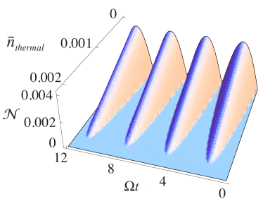
Figure 2: (Color online) Time evolution of the degree of entanglement, as measured by the logarithmic negativity, as a function of initial temperature of the movable mirrors, measured in terms of $\bar{n}_{\rm thermal}$. The dimensionless parameters are chosen such that $\Omega=1$, $g=10^{-2}$, $\lambda=10^{-1}$, $\alpha_{A}=4$ and $\alpha_{B}=1$.

III.3 Dissipative dynamics

In any physical setting, coupling to the environment is inevitable and typically results in decoherence of the quantum state to its classical counterpart. In the scheme of interest to us, there can be two main causes of dissipation. One is the photon leakage through the two cavities, and the other is thermal decay of the states of the movable mirrors due to their coupling to baths of non-zero temperature.

So far we have treated the cavity modes in the adiabatic approximation by expanding the global wave function in terms of energy eigenstates of the collective cavity operators $\hat{A}$ and $\hat{B}$. Although it might look somewhat artificial at first, this approach has its own advantages. Firstly, it allows us to derive a closed-form analytical result governing the dynamics of the two coupled mirrors, which is otherwise a nonlinear problem in itself. Secondly, it also provides us with useful physical insights into how the cavity assisted entanglement of spatially separated mechanical oscillators originates. In the present section we will continue treating the two cavity modes in this semiclassical regime and defer the explicit calculations involving reservoir induced quantum fluctuations in the cavity modes till the next section. More precisely, we assign coherent states for the two cavity modes and introduce cavity losses in terms of a non-Hermitian Hamiltonian.

A phenomenological way to introduce cavity losses is to shift the cavity resonance frequency $\omega$ by $-i\kappa$ where $\kappa$ is the cavity decay rate. Then, under the BO approximation, the two indirectly coupled movable mirrors evolve according to the non-Hermitian Hamiltonian

$$\hat{H}_{\rm disp}\approx\hat{H}_{\rm mir}-i\kappa(n_{A}+n_{B})\,,$$ (27)

where $\hat{H}_{\rm mir}$ is given by (III.1) and we again have neglected all the classical driving terms in the Hamiltonian. Apart from the cavity losses, the two cavity mirrors might undergo further decoherence due to their inevitable coupling to the external environment. The time evolution of the mixed state of the two movable mirrors obtained by tracing over the cavity field distribution takes the form

$$\hat{\rho}_{\rm mir}(t)=\!\frac{1}{\sum_{n_{A},n_{B}}N_{n_{A},n_{B}}(t)}\sum_{n_{A},n_{B}}N_{n_{A},n_{B}}(t)\hat{\rho}_{\rm mir}^{(n)}(t),$$ (28)

where

$$N_{n_{A},n_{B}}(t) = \exp\left(-|\alpha_{A}e^{-\kappa t}|^{2}\right)|\alpha_{A}e^{-\kappa t}|^{{\rm 2}n_{A}}$$

$$\times\exp\left(-|\alpha_{B}e^{-\kappa t}|^{2}\right)|\alpha_{B}e^{-\kappa t}|^{{\rm 2}n_{B}}/n_{A}!n_{B}!,$$

and $\hat{\rho}_{\rm mir}^{(n)}(t)$ is the time-evolved reduced density matrix of the two movable mirrors with the photon number difference $n=n_{A}-n_{B}$. It turns out that if both collective cavity modes are initially coherent states, this particular method of taking dissipation into account is not only accurate but also exact qjump . This is because an initial coherent state evolving in a purely dissipative channel remains a coherent state, although with an exponentially decaying amplitude coherent . The time evolution of $\hat{\rho}_{\rm mir}^{(n)}(t)$ in the Born-Markov approximation is then described by the Lindblad-type master equation mil ; stev

$$\frac{\partial}{\partial t}\hat{\rho}_{\rm mir} = -i\left[\hat{H}_{\rm mir},\hat{\rho}_{\rm mir}\right]+\frac{\Gamma}{2}\bar{n}\mathcal{L}_{c^{\dagger}}\hat{\rho}_{\rm mir}+\frac{\Gamma}{2}\bar{n}\mathcal{L}_{d^{\dagger}}\hat{\rho}_{\rm mir}$$ (30)

$$+\frac{\Gamma}{2}(\bar{n}+1)\mathcal{L}_{c}\hat{\rho}_{\rm mir}+\frac{\Gamma}{2}(\bar{n}+1)\mathcal{L}_{d}\hat{\rho}_{\rm mir},$$

where $\Gamma$ is the decay rate of each movable mirror due to its coupling to a heat bath with average thermal occupancy $\bar{n}$, and $\mathcal{L}_{x}\hat{\rho}\equiv 2\hat{x}\hat{\rho}\hat{x}^{\dagger}-\hat{x}^{\dagger}\hat{x}\hat{\rho}-\hat{\rho}\hat{x}^{\dagger}\hat{x}$. In terms of the center-of-mass mode $\hat{C}$ and relative mode $\hat{D}$, Eq. (30) can be equivalently written as

$$\frac{\partial\rho_{\rm mir}}{\partial t} = -i\left[\hat{H}_{\rm mir},\hat{\rho}_{\rm mir}\right]+\frac{\Gamma}{2}\bar{n}\mathcal{L}_{C^{\dagger}}\hat{\rho}_{\rm mir}+\frac{\Gamma}{2}\bar{n}\mathcal{L}_{D^{\dagger}}\hat{\rho}_{\rm mir}$$ (31)

$$+\frac{\Gamma}{2}(\bar{n}+1)\mathcal{L}_{C}\hat{\rho}_{\rm mir}+\frac{\Gamma}{2}(\bar{n}+1)\mathcal{L}_{D}\hat{\rho}_{\rm mir},$$

where $\hat{H}_{\rm mir}$ is given by (12).

To solve the master equation (31), we define the normal-ordered quantum characteristic function mil ; stev for the two movable mirrors as $\chi(\epsilon,\eta,t)=\langle e^{\epsilon\hat{C}^{\dagger}}e^{-\epsilon^{*}\hat{C}}e^{\eta\hat{D}^{\dagger}}e^{-\eta^{*}\hat{D}}\rangle$. Using standard quantum optical techniques mil ; stev , the master equation (31) can be rewritten as a partial differential equation for the quantum characteristic function $\chi(\epsilon,\eta,t)$ of the form

$$\frac{\partial}{\partial t}\chi(\epsilon,\eta,t)=z^{T}{\mbox{\bf M}}\nabla\chi(\epsilon,\eta,t)+\rm{4}\lambda\it{z}^{T}{\mbox{\bf K}}\it{z}\chi(\epsilon,\eta,t),$$ (32)

where

$$\begin{array}[]{l}z^{T}=(u_{1},u_{2},v_{1},v_{2}),\\ \\ \nabla=\left(\frac{\partial}{\partial u_{1}},\frac{\partial}{\partial u_{2}},\frac{\partial}{\partial v_{1}},\frac{\partial}{\partial v_{2}}\right)^{T},\\ \\ u_{1}=\frac{\epsilon_{c}+\epsilon_{d}+\epsilon_{c}^{*}+\epsilon_{d}^{*}}{2\sqrt{2}},\\ \\ u_{2}=\frac{\epsilon_{c}+\epsilon_{d}-\epsilon_{c}^{*}-\epsilon_{d}^{*}}{i2\sqrt{2}},\\ \\ v_{1}=\frac{\epsilon_{c}-\epsilon_{d}+\epsilon_{c}^{*}-\epsilon_{d}^{*}}{2\sqrt{2}},\\ \\ v_{2}=\frac{\epsilon_{c}-\epsilon_{d}-\epsilon_{c}^{*}+\epsilon_{d}^{*}}{i2\sqrt{2}},\end{array}$$ (33)

and

$$\epsilon_{c}=\frac{\epsilon+\eta}{\sqrt{2}}, \epsilon_{d}=\frac{\epsilon-\eta}{\sqrt{2}}.$$ (34)

The $4\times 4$ matrix coefficients of Eq. (32) read

$$\begin{array}[]{llll}{\mbox{\bf M}}=\left(\begin{array}[]{cc}{\mbox{\bf M}_{1}}&{\mbox{\bf 0}}\\ {\mbox{\bf 0}}&{\mbox{\bf M}_{2}}\\ \end{array}\right),&&&{\mbox{\bf K}}=\left(\begin{array}[]{cc}{\mbox{\bf K}_{1}}&{\mbox{\bf 0}}\\ {\mbox{\bf 0}}&{\mbox{\bf K}_{2}}\\ \end{array}\right),\end{array}$$ (35)

with

$$\begin{array}[]{l}{\mbox{\bf M}_{1}}=\left(\begin{array}[]{cc}{-\Gamma/2}&{\Omega}\\ {-\Omega}&{-\Gamma/2}\\ \end{array}\right),\\ \\ {\mbox{\bf M}_{2}}=\left(\begin{array}[]{cc}{-\Gamma/2}&{\Omega-8N\lambda}\\ {-\Omega}&{-\Gamma/2}\\ \end{array}\right),\\ \\ {\mbox{\bf K}_{1}}=\left(\begin{array}[]{cc}{-\Gamma\bar{n}/4\lambda}&{0}\\ {0}&{-\Gamma\bar{n}/4\lambda}\\ \end{array}\right),\\ \\ {\mbox{\bf K}_{2}}=\left(\begin{array}[]{cc}{-\Gamma\bar{n}/4\lambda}&{N}\\ {N}&{-\Gamma\bar{n}/4\lambda}\\ \end{array}\right).\end{array}$$ (36)

For an initial Gaussian state of the two movable mirrors, it is consistent to make the following Ansatz for the quantum characteristic function,

$$\chi(\epsilon,\eta,t)=\exp\left[-z^{T}{\mbox{\bf L}}(t)\,z+iz^{T}q(t)\right],$$ (37)

where ${\mbox{\bf L}}(t)$ is a $4\times 4$ time-dependent symmetric matrix and $q(t)$ is a $4\times 1$ time-dependent vector. Using the above Ansatz in Eq. (32) results in the coupled matrix differential equations

$$\dot{{\mbox{\bf L}}} = {\mbox{\bf M}}{\mbox{\bf L}}+{\mbox{\bf L}}{\mbox{\bf M}}^{T}-4\lambda{\mbox{\bf K}},$$ (38)

$$\dot{q} = {\mbox{\bf M}}q.$$ (39)

Making use of the fact that L is a $4\times 4$ symmetric matrix, it can be decomposed into $2\times 2$ square matrices such that

$${\mbox{\bf L}}=\left(\begin{array}[]{cc}{{\mbox{\bf P}}}&{{\mbox{\bf Q}}}\\ {{\mbox{\bf Q}^{T}}}&{{\mbox{\bf R}}}\\ \end{array}\right),$$ (42)

where P and R are 2$\times$2 symmetric matrices. Obtaining an explicit form for the time-dependent quantum characteristic function $\chi(\epsilon,\eta,t)$ now reduces to solving $2\times 2$ coupled matrix differential equations.

Although an exact analytical solution can be arrived at, it is too lengthy to be reported here. Nonetheless, the time-dependent covariance matrix V can be fully reconstructed from the quantum characteristic function $\chi(\epsilon,\eta,t)$. This can be easily seen by noting that from the quantum characteristic function one can obtain the expectation values of quantum mechanical observables, e.g., $\langle\hat{c}^{\dagger m}(t){\it\hat{d}^{\dagger n}}(t)\rangle=\it{(\frac{\partial}{\partial\epsilon_{c}})^{m}(\frac{\partial}{\partial\epsilon_{d}})^{n}\chi(\epsilon_{c},\epsilon_{d},t)}|_{\it{\epsilon_{c},\epsilon_{d}}=\rm{0}}$ and thus all the elements of the covariance matrix can be found.

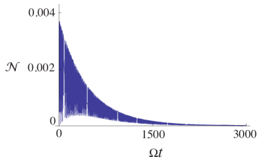
Figure 3: (Color online) Temporal evolution of the degree of entanglement between two indirectly coupled movable mirrors as measured by the logarithmic negativity. Compared with Fig. 2, here losses in all modes have been considered and the degree of entanglement is consequently somewhat smaller, but importantly, it survives for a reasonably long time. Each mirror is initially assumed to be in its ground state and the dimensionless parameters used are chosen such that $\Omega=1$, $g=10^{-2}$, $\lambda=10^{-1}$, $\alpha_{A}=4$, $\alpha_{B}=1$, $\kappa=10^{-3}$, $\Gamma=10^{-4}$ and $\bar{n}=0$.

As a measure of entanglement between the distant cavity mirrors we again compute the logarithmic negativity. The result of such a calculation is shown in Fig. 3. As is clear from the figure, under the action of cavity-mediated coupling, the two movable mirrors exhibit entanglement. Although the entanglement generated is not too large, it is sustained over a reasonably long timescale. The degree of inseparability between the two mirrors can be improved significantly either by a conditional measurement of the cavity field or by increasing the difference in the mean number of photons in the field distributions of the two cavity modes. Thus we conclude that the aforementioned protocol is indeed capable of generating quantum entangled states of two movable mirrors, which are robust with respect to dissipation for a long time. It should be pointed out that the logarithmic negativity approaches zero exponentially for large times due to the decay of photons out of the cavities. In order to have sustainable non-vanishing entanglement, the photon modes must be driven externally to prevent the absence of photons. This will be discussed in the following section.

III.4 Validity of the Born-Oppenheimer approximation

So far we have used the BO approximation to separate the slow dynamics of the two movable mirrors from the rapidly evolving population of the two cavity modes. The BO approach has proved to be a fundamental tool in various applications of physics and quantum chemistry BO ; lsced . It is nothing but an extension of the quantum adiabatic theorem to a quantum system with two sets of variables whose dynamics can be separated due to very different dynamical time scales.

The original version of the adiabatic theorem asserts that an initial eigenstate of a slowly varying Hamiltonian will remain in the same instantaneous eigenstate throughout the evolution. In our system, the absence of transitions between instantaneous eigenstates translates to fixed probabilities for the states $|n\rangle$, see Eq. (7), to be occupied. There has been continued interest in the application of the adiabatic theorem in slowly evolving quantum mechanical systems including Berry’s phase and effective gauge theories berry ; gauge , geometric quantum computation geom , and adiabatic quantum computation adiaba . However, recently the generally accepted criteria for adiabaticity in quantum physics has suffered some criticisms criti , which has lead to various arguments and counter-arguments to ascertain the justification of the adiabatic approximation in quantum theory dmtong ; mhsamin . A breakdown of adiabaticity seems to appear only in rather special cases of rapid resonant driving of the system mhsamin . This kind of external resonant driving is absent in our model and we expect a standard application of the adiabatic theorem, or more precisely an application of the BO approximation, to be unproblematic. In the beginning of Sec. III.1, we pointed out that the two types of oscillators evolve on very different time scales which normally guarantees adiabatic dynamics. However, one issue overlooked so far concerns the fact that we consider an open quantum system for which the concept of adiabaticity must be handled with care xlhunag . Loosely speaking, one could imagine non-adiabatic transitions induced by the reservoir. In the following discussion we will argue that such transitions are indeed not present in our model.

Recently an extension of the BO approximation has been presented for a quantum system coupled to a large reservoir xlhunag . Following this work, we can write the Hamiltonian of the closed quantum system as $H=H_{s}(X)+H_{f}(X,Y)$, where $H_{s}(X)$ is the Hamiltonian of the slowly varying dynamical variable $X$ and $H_{f}(X,Y)$ is the interaction Hamiltonian between the slowly varying variable and the quickly varying dynamical variable $Y$. If the coupling between the quantum system and the reservoir is such that its evolution can be described using the Lindblad approach, then, in the case of no quantum jumps, the evolution of the quantum system is governed by the equation

$$i\hbar\frac{d}{dt}|\Psi(t)\rangle=H_{\rm eff}|\Psi(t)\rangle.$$ (43)

Here $H_{\rm eff}=H_{s}(X)+H_{f}^{\prime}(X,Y)$, and $H_{f}^{\prime}(X,Y)$ is the non-hermitian part of the Hamiltonian, with dissipation assumed to affect only the quickly varying variable of the Hamiltonian. Treating the slowly varying variable $X$ as a parameter, we can solve for left and right eigenstates $\langle\Psi_{n,X}^{L}(Y)|$ and $|\Psi_{n,X}^{R}(Y)\rangle$ of the non-hermitian Hamiltonian $H_{f}^{\prime}(X,Y)$, with complex eigenvalues $E_{n,X}(Y)$. Expanding the eigenstates of $H_{\rm eff}$ in terms of $|\Psi_{n,X}^{R}(Y)\rangle$ we get

$$|\Phi\rangle=\sum_{n=1}^{N}c_{n}|\varphi_{n}(X)\rangle|\Psi_{n,X}^{R}(Y)\rangle,$$ (44)

where $N$ is the dimension of the quickly varying variable $Y$ and $c_{n}$ are the expansion coefficients. It can be shown that the eigenvalue equation $H_{\rm eff}|\Phi\rangle=E|\Phi\rangle$ can be recast in the form $(H_{o}+H_{P})\varphi=E\varphi$ xlhunag , where

$$H_{o}(X)\! = \!\!\left[\begin{array}[]{cccc}\!H_{1}\!+\!E_{1}(Y)&0&\cdots&0\\ 0&H_{2}\!+\!E_{2}(Y)&\cdots&0\\ \vdots&\vdots&\ddots&\vdots\\ 0&0&\cdots&H_{N}\!+\!E_{N}(Y)\!\end{array}\right]\!,$$

$$H_{P}(X) = \left[\begin{array}[]{cccc}0&H_{1,2}&\cdots&H_{1,N}\\ H_{2,1}&0&\cdots&H_{2,N}\\ \vdots&\vdots&\ddots&\vdots\\ H_{N,1}&H_{N,2}&\cdots&0\end{array}\right],~{}~{}\varphi=\left[\begin{array}[]{c}|\varphi_{1}\rangle\\ |\varphi_{2}\rangle\\ \vdots\\ |\varphi_{N}\rangle\end{array}\right]$$

Here $H_{n}=H_{n,n}$, $E_{n}(Y)=E_{n,X}(Y)$ and $H_{n,m}(X)=\langle\Psi_{n,X}^{L}(Y)|H_{s}(X)|\Psi_{n,X}^{R}(Y)\rangle$. Treating $H_{P}$ as a small perturbation and using standard time independent perturbation theory, corrections to all orders for the eigenstates and the eigenenergies can be calculated. Since there is no resonant driving, we can conclude that the BO approximation is accurate as long as the condition

$$\left|\frac{\langle\Phi_{n^{\prime},k^{\prime}}^{L[0]}|H_{n^{\prime},n}|\Phi_{n,k}^{R[0]}\rangle}{E_{n^{\prime},k^{\prime}}^{[0]}-E_{n,k}^{[0]}}\right|<<1~{}~{}~{}~{}~{}~{}~{}{\rm for~{}all~{}}~{}k^{\prime},n^{\prime}\neq k,n.$$ (47)

is satisfied xlhunag .

Returning to consider our original physical system of two coupled optomechanical cavities, the non-hermitian Hamiltonian containing the cavity decay terms takes the form

$$\hat{H}_{\rm{cav}} = {\hbar\left(\omega-i\kappa-g\frac{\hat{q}_{1}+\hat{q}_{2}}{2}\right)(\hat{A}^{\dagger}\hat{A}+\hat{B}^{\dagger}\hat{B})}$$ (48)

$${-\hbar\sqrt{g^{2}{\left(\hat{q}_{1}-\hat{q}_{2}\right)^{2}+4\lambda^{2}}}\frac{(\hat{A}^{\dagger}\hat{A}-\hat{B}^{\dagger}\hat{B})}{2}}$$

$${+\hbar\frac{\Omega}{2}(\hat{q}_{1}^{2}+\hat{p}_{1}^{2}+\hat{q}_{2}^{2}+\hat{p}_{2}^{2})}.$$

The quickly varying part of the Hamiltonian

$$H_{f} = \hbar\left[\omega-i\kappa-g(\hat{q}_{1}+\hat{q}_{2})/2\right](\hat{A}^{\dagger}\hat{A}+\hat{B}^{\dagger}\hat{B})-$$

$$\hbar\sqrt{g^{2}{\left(\hat{q}_{1}-\hat{q}_{2}\right)^{2}+4\lambda^{2}}}(\hat{A}^{\dagger}\hat{A}-\hat{B}^{\dagger}\hat{B})/2$$

has left and right eigenstates $\langle\Psi_{n,X}^{L}(Y)|=\langle n_{A}|\langle n_{B}|$ and $|\Psi_{n,X}^{R}(Y)\rangle=|n_{A}\rangle|n_{B}\rangle$ respectively, with complex eigenvalues given by

$$E_{n,X}(Y) = \hbar(\omega-i\kappa-g(\hat{q}_{1}+\hat{q}_{2})/2)(n_{A}+n_{B})-$$

$$\hbar\sqrt{g^{2}(\hat{q}_{1}-\hat{q}_{2})^{2}+4\lambda^{2}}(n_{A}-n_{B})/2.$$

As a passing remark, the perturbation terms $H_{P}$ are in general non-zero. This demands that the dissipation in the slowly varying variables must be slower than the dissipation in the quickly varying variables. If this condition is not met, then strong dissipation in the slowly varying variables enlarges the perturbation $H_{P}$, which might make the BO approximation invalid. Roughly speaking, a stronger rate of dissipation in the slowly varying variables accelerates their rate of change, thus making it hard to distinguish their dynamics from that of the quickly varying variables. The slowly varying variables then evolve under the effective Hamiltonian

$$\hat{H}_{\rm mirror} = \hbar\frac{\Omega}{2}\left(\hat{q}_{1}^{2}+\hat{p}_{1}^{2}+\hat{q}_{2}^{2}+\hat{p}_{2}^{2}\right)$$ (49)

$$-\hbar\sqrt{g^{2}{\left(\hat{q}_{1}-\hat{q}_{2}\right)^{2}+4\lambda^{2}}}\frac{(n_{A}-n_{B})}{2}$$

$$+\hbar\left(\omega-i\kappa-g\frac{\hat{q}_{1}+\hat{q}_{2}}{2}\right)(n_{A}+n_{B}).$$

It should be noticed that in this treatment, the off-diagonal terms of the perturbation $H_{P}$, which are given by $H_{n,m}(X)=\langle n_{A}|\langle n_{B}|\hat{H}_{\rm mirror}|m_{A}\rangle|m_{B}\rangle$, are identically zero. This implies that the zeroth order BO approximation for this particular physical model is not only accurate but also exact. The conclusion remains the same even when dissipation in the slow variables is taken into account xlhunag .

IV Quantum Langevin approach

As mentioned before, in a typical optomechanical setup, due to coupling induced by radiation pressure, a movable mirror interacts with a cavity mode. Unfortunately, the radiation pressure coupling for an undriven cavity with a movable mirror is usually very weak. This problem can be circumvented by driving the cavity with a coherent classical laser field. Driving with an intense laser field enhances the radiation pressure coupling and thus facilitates the observation of non-classical phenomena such as entanglement between mechanical oscillators and light.

In the previous section, cavity driving was not taken into account. Instead the two cavity fields were assumed to be initially in coherent states and the system time-evolution in the presence of the decay of the two cavity fields was studied. In what follows, we shall instead study the situation of cavity driving and show that robust steady state entanglement may exist between different optical and mechanical modes. To this end, we find it more convenient to work in the Heisenberg picture. For our system of two coupled cavities with movable mirrors, the Hamiltonian in the interaction picture of the two driving lasers with frequency $\omega_{L}$ now takes the form

$$\frac{\hat{H}}{\hbar} = (\omega-\omega_{L})(\hat{a}^{\dagger}\hat{a}+\hat{b}^{\dagger}\hat{b})+\frac{\Omega}{2}(\hat{q}_{1}^{2}+\hat{p_{1}}^{2})+\frac{\Omega}{2}(\hat{q}_{2}^{2}+\hat{p}_{2}^{2})$$ (50)

$$+\lambda(\hat{a}^{\dagger}\hat{b}+\hat{b}^{\dagger}\hat{a})-g\hat{a}^{\dagger}\hat{a}\hat{q_{1}}-g\hat{b}^{\dagger}\hat{b}\hat{q_{2}}$$

$$+i\eta(\hat{a}^{\dagger}-\hat{a})+i\eta(\hat{b}^{\dagger}-\hat{b}).$$

Here $\eta=\sqrt{2P_{c}\kappa/\hbar\omega_{c}}$ is related to the driving laser, where $P_{c}$ is the power of the driving laser and $\kappa$ is the damping rate, identical for both cavities.

The Hamiltonian (50) describes the closed-system dynamics of the two driven coupled cavities with movable mirrors. However, as discussed in the previous section, the dynamics of the system is also affected by damping and noise. The main channels of dissipation in our system are the decay in the cavity modes and the coupling of the movable mirrors to their independent thermal baths combath . One possible way to take into account all the damping and noise processes is to use quantum Langevin equations (QLEs). The QLEs are equivalent to the Heisenberg equations of motion for time-evolving operators, where noise and dissipative processes have been included phenomenologically mil .

For the Hamiltonian (50), the QLEs for the cavity and the mirror modes become

$$\begin{array}[]{l}\frac{d\hat{a}}{dt}=-i\lambda\hat{b}+ig\hat{q}_{1}\hat{a}+\eta-(\kappa+i\tilde{\Delta})\hat{a}+\sqrt{2\kappa}\hat{a}_{in},\\ \\ \frac{d\hat{b}}{dt}=-i\lambda\hat{a}+ig\hat{q}_{2}\hat{b}+\eta-(\kappa+i\tilde{\Delta})\hat{b}+\sqrt{2\kappa}\hat{b}_{in},\\ \\ \frac{d\hat{p}_{1}}{dt}=-\Omega\hat{q}_{1}+g\hat{a}^{\dagger}\hat{a}-\gamma_{m}\hat{p}_{1}+\hat{\varepsilon}_{1}(t),\\ \\ \frac{d\hat{p}_{2}}{dt}=-\Omega\hat{q}_{2}+g\hat{b}^{\dagger}\hat{b}-\gamma_{m}\hat{p}_{2}+\hat{\varepsilon}_{2}(t),\\ \\ \frac{d\hat{q}_{1}}{dt}=\Omega\hat{p}_{1},\\ \\ \frac{d\hat{q}_{2}}{dt}=\Omega\hat{p}_{2},\end{array}$$ (51)

where $\tilde{\Delta}=\omega-\omega_{L}$ is the laser detuning from the cavity resonance frequency $\omega$, $\kappa$ is the decay rate of each cavity and $\gamma_{m}$ is the thermal decay rate, identical for the two movable mirrors subjected to independent Brownian motion noise characterized by the operators $\hat{\varepsilon}_{1}(t)$ and $\hat{\varepsilon}_{2}(t)$ respectively. The quantum noise operators have the quantum statistical properties

$$\langle\hat{\varepsilon}_{1}(t)\rangle = \langle\hat{\varepsilon}_{2}(t)\rangle=0,$$ (52)

$$\langle\hat{\varepsilon}_{i}(t)\hat{\varepsilon}_{j}(t^{\prime})\rangle = \frac{\gamma_{m}}{\Omega}\int e^{-i\omega^{{}^{\prime}}(t-t^{{}^{\prime}})}\omega^{{}^{\prime}}$$

$$\times\left[1+\coth\left(\frac{\hbar\omega^{{}^{\prime}}}{k_{B}T_{i}}\right)\right]\frac{d\omega^{{}^{\prime}}}{2\pi}\delta_{ij},$$

where $i,\,j\in 1,\,2$ and $\delta_{ij}$ is the Kronecker delta. We have also introduced independent cavity input noise operators, $\hat{a}_{in}(t)$ and $\hat{b}_{in}(t)$ for the first and second cavity respectively. For the case of optical fields, $\hbar\omega/k_{B}T\gg 1$, and hence the mean number of thermal photons can be safely neglected. In this limit the noise operators $\hat{a}_{in}(t)$ and $\hat{b}_{in}(t)$ satisfy the two-time correlations

$$\begin{array}[]{l}\langle\hat{a}_{in}(t)\hat{a}^{\dagger}_{in}(t^{\prime})\rangle=\delta(t-t^{\prime}),\\ \\ \langle\hat{a}^{\dagger}_{in}(t)\hat{a}_{in}(t^{\prime})\rangle=0,\\ \\ \langle\hat{b}_{in}(t)\hat{b}^{\dagger}_{in}(t^{\prime})\rangle=\delta(t-t^{\prime}),\\ \\ \langle\hat{b}^{\dagger}_{in}(t)\hat{b}_{in}(t^{\prime})\rangle=0.\end{array}$$ (53)

We are interested in investigating the possibility of achieving steady-state entanglement between distant optical and mechanical modes. To pursue this aim we have to solve the set of coupled nonlinear QLEs (51). This task is difficult, but it is simplified in the presence of strong external driving, in which case linearization of the set of QLEs around the steady-state values is justified. Solving the set of QLEs (51) for the steady-state amplitudes of the optical and mechanical modes, we get

$$\begin{array}[]{l}q_{1}^{s}=\frac{g|a_{s}|^{2}{\Omega}}{,}\\ \\ q_{2}^{s}=\frac{g|b_{s}|^{2}{\Omega}}{,}\\ \\ p_{1}^{s}=0,\\ \\ p_{2}^{s}=0,\\ \\ {a}_{s}=\frac{-i\lambda\eta+\eta(\kappa+i\Delta_{b})}{\lambda^{2}+\kappa^{2}+i\kappa(\Delta_{a}+\Delta_{b})-\Delta_{a}\Delta_{b}},\\ \\ {b}_{s}=\frac{-i\lambda\eta+\eta(\kappa+i\Delta_{a})}{\lambda^{2}+\kappa^{2}+i\kappa(\Delta_{a}+\Delta_{b})-\Delta_{a}\Delta_{b}},\\ \\ \Delta_{a}=\tilde{\Delta}-gq_{1}^{s}=\omega-\omega_{L}-gq_{1}^{s},\\ \\ \Delta_{b}=\tilde{\Delta}-gq_{2}^{s}=\omega-\omega_{L}-gq_{2}^{s}.\end{array}$$ (54)

In the regime where the two cavities are very intensely driven, such that $|a_{s}|,|b_{s}|\gg 1$, and by expanding the mechanical and optical mode operators as quantum fluctuations around the steady state values ($\hat{a}=a_{s}+\delta\hat{a}$, $\hat{b}=b_{s}+\delta\hat{b}$, $\hat{q}_{i}=q_{i}^{s}+\delta\hat{q}_{i}$ and $\hat{p}_{i}=p_{i}^{s}+\delta\hat{p}_{i}$ for $i=1,2$) we obtain the following linearized QLEs for the quantum fluctuations,

$$\begin{array}[]{l}\frac{d\delta\hat{a}}{dt}=-\delta\hat{a}(\kappa+i\Delta_{a})-i\lambda\delta\hat{b}+iga_{s}\delta\hat{x}+\sqrt{2\kappa}\hat{a}_{in},\\ \\ \frac{d\delta\hat{b}}{dt}=-\delta\hat{b}(\kappa+i\Delta_{b})-i\lambda\delta\hat{a}+igb_{s}\delta\hat{y}+\sqrt{2\kappa}\hat{b}_{in},\\ \\ \frac{d\delta\hat{q}_{1}}{dt}=\Omega\delta\hat{p}_{1},\\ \\ \frac{d\delta\hat{q}_{2}}{dt}=\Omega\delta\hat{p}_{2},\\ \\ \frac{d\delta\hat{p}_{1}}{dt}=-\Omega\delta\hat{q}_{1}+g\left(|a_{s}|^{2}+a_{s}^{*}\delta\hat{a}+a_{s}\delta\hat{a}^{\dagger}\right),\\ \\ \frac{d\delta\hat{p}_{2}}{dt}=-\Omega\delta\hat{q}_{2}+g\left(|b_{s}|^{2}+b_{s}^{*}\delta\hat{b}+b_{s}\delta\hat{b}^{\dagger}\right).\end{array}$$ (55)

By further introducing the position and momentum quadratures for the two cavity modes and their input noises,

$$\frac{d\delta\hat{X}_{a}}{dt} = \frac{d(\delta\hat{a}^{\dagger}+\delta\hat{a})}{dt},$$ (56)

$$\frac{d\delta\hat{P}_{a}}{dt} = i\frac{d(\delta\hat{a}^{\dagger}-\delta\hat{a})}{dt},$$

$$\frac{d\delta\hat{X}_{b}}{dt} = \frac{d(\delta\hat{b}^{\dagger}+\delta\hat{b})}{dt},$$

$$\frac{d\delta\hat{P}_{b}}{dt} = i\frac{d(\delta\hat{b}^{\dagger}-\delta\hat{b})}{dt},$$

$$\frac{d\delta\hat{X}_{in}^{a}}{dt} = \frac{d(\delta\hat{a}_{in}^{\dagger}+\delta\hat{a}_{in})}{dt},$$

$$\frac{d\delta\hat{P}_{in}^{a}}{dt} = i\frac{d(\delta\hat{a}_{in}^{\dagger}-\delta\hat{a}_{in})}{dt},$$

$$\frac{d\delta\hat{X}_{in}^{b}}{dt} = \frac{d(\delta\hat{b}_{in}^{\dagger}+\delta\hat{b}_{in})}{dt},$$

$$\frac{d\delta\hat{X}_{in}^{b}}{dt} = i\frac{d(\delta\hat{b}_{in}^{\dagger}-\delta\hat{b}_{in})}{dt},$$

we can rewrite Eq. (55) in the compact form

$$\frac{dR}{dt}={\mbox{\bf Z}}R+N.\\$$ (57)

Here

$$\begin{array}[]{lll}R^{T}&=&\big{(}\delta\hat{q}_{1},\delta\hat{p}_{1},\delta\hat{q}_{2},\delta\hat{p}_{2},\delta\hat{X}_{a},\delta\hat{P}_{a},\delta\hat{X}_{b},\delta\hat{P}_{b}\big{)},\\ \\ N^{T}&=&\big{(}0,\epsilon_{1}(t),0,\epsilon_{2}(t),\sqrt{2\kappa}\delta\hat{X}_{in}^{a}(t),\\ \\ &&\sqrt{2\kappa}\delta\hat{P}_{in}^{a}(t),\sqrt{2\kappa}\delta\hat{X}_{in}^{b}(t),\sqrt{2\kappa}\delta\hat{P}_{in}^{b}(t)\big{)},\end{array}$$ (58)

and

Z $$= \left(\begin{array}[]{cc}{\mbox{\bf Z}_{1}}&{\mbox{\bf Z}_{2}}\\ {\mbox{\bf Z}_{2}}&{\mbox{\bf Z}_{3}}\\ \end{array}\right),$$

with the $4\times 4$ matrices

$$\begin{array}[]{l}{\mbox{\bf Z}_{1}}=\left(\begin{array}[]{cccc}0&\Omega&0&0\\ -\Omega&-\gamma_{m}&0&0\\ 0&0&0&\Omega\\ 0&0&-\Omega&-\gamma_{m}\\ \end{array}\right),\\ \\ {\mbox{\bf Z}_{2}}=\left(\begin{array}[]{cccc}0&0&0&0\\ g_{a}^{s}&0&0&0\\ 0&0&0&0\\ 0&0&g_{b}^{s}&0\\ \end{array}\right),\\ \\ {\mbox{\bf Z}_{3}}=\left(\begin{array}[]{cccc}-\kappa&\Delta_{a}&0&\lambda\\ -\Delta_{a}&-\kappa&-\lambda&0\\ 0&\lambda&-\kappa&\Delta_{b}\\ -\lambda&0&-\Delta_{b}&-\kappa\\ \end{array}\right).\end{array}$$ (60)

The phase reference has been chosen such that $a_{s}$ and $b_{s}$ are real with $g_{a}^{s}=\sqrt{2}ga_{s}$ and $g_{b}^{s}=\sqrt{2}gb_{s}$. In Eq. (57), Z is the drift matrix. Stability (in the steady state) demands that the real part of all the eigenvalues of Z must be negative. All the parameters in the present work have been chosen such that the system is stable in the steady state.

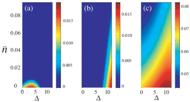
Figure 4: (Color online) Logarithmic negativity as a measure of entanglement between (a) two distant cavity mirrors, (b) a mirror and adjacent cavity mode, and (c) a mirror and distant cavity mode, plotted as a function of detuning $\Delta$ and average thermal occupancy of the two mirrors $\bar{n}_{1}=\bar{n}_{2}=\bar{n}$. We have chosen the different physical parameters such that $\Omega=1$, $g_{a}^{s}=g_{b}^{s}=2.5$, $\lambda=20$, $\kappa=0.08$, $\gamma_{m}=0.01$, and $\Delta_{a}=\Delta_{b}=\Delta$

The dynamics of the coupled cavities with movable mirrors is governed by the first order matrix differential equation (57). For an initial Gaussian state of the two cavities and their movable mirrors it is sufficient to fully characterize all the quantum correlations by explicitly evaluating the $8\times 8$ symmetric covariance matrix V where $V_{i,j}(t)=(\langle R_{i}(t)R_{j}(t)+R_{j}(t)R_{i}(t)\rangle)/2$. If the system is stable in the steady state, then the covariance matrix takes the form

$$V_{i,j}=\sum_{p,q}\int_{0}^{\infty}{ds}\int_{0}^{\infty}{ds^{\prime}}W_{i,p}(s)W_{j,q}(s^{\prime})\Phi_{p,q}(s-s^{\prime}),$$ (61)

where ${\mbox{\bf W}}=\rm{exp}(\mbox{\bf Z}s)$ and $\Phi_{p,q}(s-s^{\prime})=(\langle N_{p}(s)N_{q}(s^{\prime})+N_{q}(s^{\prime})N_{p}(s)\rangle)/2$ is the steady-state noise correlation matrix. It turns out that in the regime where the mechanical oscillators possess very high $Q$-values, the quantum Brownian noise becomes approximately $\delta$-correlated and in this limit the noise correlation matrix takes the form

$$\begin{array}[]{l}\Phi_{p,q}(s-s^{\prime})=\tilde{N}_{p,q}\delta(s-s^{\prime}),\\ \\ \begin{array}[]{lll}&=&\rm{Diag}[0,\gamma_{m}(2\bar{n}_{1}+1)),0,\gamma_{m}(2\bar{n}_{2}+1),\\ \\ &&\kappa,\kappa,\kappa,\kappa]\delta(s-s^{\prime}),\end{array}\end{array}$$ (62)

with $\bar{n}_{1}=\left[e^{(\hbar\Omega/k_{B}T_{1})}-1\right]^{-1}$ and $\bar{n}_{2}=\left[e^{(\hbar\Omega/k_{B}T_{2})}-1\right]^{-1}$. Thus, Eq. (61) simplifies to

$${\mbox{\bf V}}=\int_{0}^{\infty}{ds}{\mbox{\bf W}}(s)\tilde{{\mbox{\bf N}}}{\mbox{\bf W}}^{T}(s).$$ (63)

When the system is stable in the steady state, the covariance matrix V satisfies a Lyapunov equation smans3

$${\mbox{\bf Z}}{\mbox{\bf V}}+{\mbox{\bf V}}{\mbox{\bf Z}}^{T}=-\tilde{{\mbox{\bf N}}}.$$ (64)

Once again, when we have the solution for the covariance matrix, we can compute various non-classical correlations between the optical and mechanical degrees of freedom. In particular, the degree of entanglement between different optical and mechanical modes can be evaluated by computing the logarithmic negativity as defined in (25). We numerically solve Eq. (64) for the covariance matrix $V$. An example of the numerically calculated logarithmic negativity between various optical and mechanical modes is presented in Fig. 4.

For evaluating the entanglement between various optical and mechanical modes we have chosen physical parameters accessible in present experiments. Not surprisingly, the steady-state entanglement is susceptible to thermal fluctuations of the environment. A high temperature of the surrounding reservoirs will result in a completely separable state of the optical and mechanical modes. One should note that the entanglement generated between optical and mechanical modes in the steady state is not very large, but, it does not require any quantum resources, such as additionally driving the two cavities with squeezed light agarwal ; laura .

Also, it is worth pointing out that with our particular choice of parameters we find that an appreciable entanglement appears between various optical and mechanical modes only when we operate far away from the regime of the red ($\Delta=\Omega$) or blue ($\Delta=-\Omega$) sideband. Although operating in the blue sideband regime is commonly considered ideal for generating entanglement between various optical and mechanical modes, the condition that the steady state should be stable puts serious restrictions on the coupling strength between the mechanical and optical modes dvittwo .

A challenging aspect of any scheme involving entanglement generation between macroscopic mechanical systems is the actual experimental detection of entanglement. There are however some recent promising proposals to create and detect quantum correlations in optomechanical settings laura ; mfent . Since it is comparatively easier to detect quantum correlations between optical modes, as compared to directly detecting quantum entanglement between mechanical modes, the essence of these proposals is to swap the nonlocal correlations from the mechanical modes back to the optical modes. As shown in Fig. 1 this can, for instance, be implemented using two auxiliary light modes, each initially prepared in classical uncorrelated states. These auxiliary modes can be two modes of distant cavities, and the geometry so arranged that each entangled mirror couples independently to the two modes. The non-local correlations may then be transferred from the movable mirrors to the initially uncorrelated auxiliary modes, which may eventually become entangled. Thus, using standard homodyne measurement techniques, the entire correlation matrix of the two optical auxiliary modes can be reconstructed. A presence of non-zero quantum correlations between these optical modes will be an indirect signature of non-zero quantum correlations between the mechanical modes.

V Conclusion

We have discussed in detail the possibility of generating nonlocal quantum correlations between optical and mechanical modes of two spatially separated cavities. Each cavity is assumed to have one fixed and one movable mirror and the two cavities are coupled by an optical fiber. Under the Born-Oppenheimer approximation, relying on separating the dynamics into a fast optical timescale and a slow mechanical timescale, we have analytically worked out the dynamics of the two coupled movable mirrors. Furthermore, within this adiabatic regime, we have also presented a full analytical solution of the master equation governing the open-system dynamics of the two movable mirrors. We especially found that the interaction mediated via two optical modes entangles the two distant movable mirrors. Cavity losses were taken into account in an effective non-Hermitian model, and mirror entanglement was found to be fairly robust against such dissipation. Using a complementary model, we have studied the two coupled cavities using the quantum Langevin formalism, by explicitly solving the resulting equations of motion. In the presence of strong driving laser fields we have found that the two coupled cavities exhibit nonlocal quantum correlations between distant optical and mechanical modes. In particular, these optical and mechanical modes exhibit entanglement in the steady state and at finite temperatures. This opens up an interesting possibility to study spatially separated massive Schrödinger cat states.

During the completion of this work we became aware of a recent proposal discussing the possibility of phonon photon entanglement in coupled optomechanical arrays akram2 .

VI Acknowledgements

We gratefully acknowledge fruitful discussions with U. Akram and G. J. Milburn. C.J. acknowledges Michael Hall for introducing him to an alternative way to solve the master equation and also support from the ORS scheme. J.L. acknowledges financial support from the Swedish Research Council (VR), Deutscher Akademischer Austausch Dienst (DAAD), and Kungl. Vetenskapsakademien (KVA), M.J. support from the Swedish Research Council (VR) and the Korean WCU program funded by MEST/KOSEF (R31-2008-000-10057-0), and E.A. acknowledges support from EPSRC EP/G009821/1.

References

• (1) E. Schrödinger, Naturwissenschaften 23, 807-812; 823-823; 844-849 (1935).
• (2) W. H. Zurek, Rev. Mod. Phys. 75, 715 (2003).
• (3) J. R. Friedman, V. Patel, W. Chen, S. K. Tolpygo and J. E. Lukens, Nature (London) 406, 43 (2000).
• (4) H. M. Wiseman and G. J. Milburn, Quantum Measurement and Control, (Cambridge University Press, Cambridge, 2009).
• (5) F. Marquardt and S. M. Girvin, Physics 2, 40 (2009).
• (6) T. J. Kippenberg and K. J. Vahala, Science 321, 1172 (2008).
• (7) T. J. Kippenberg and K. J. Vahala, Optics Express 15, 17172 (2007).
• (8) T. J. Kippenberg, H. Rokhsari, T. Carmon, A. Sherer, and K. J. Vahala, Phys. Rev. Lett. 95, 033901 (2005).
• (9) A. Dorsel, J. D. McCullen, P. Meystre, E. Vignes, and H. Walther, Phys. Rev. Lett. 51, 1550 (1983).
• (10) S. Gröblacher, K. Hammerer, M. R. Vanner, and M. Aspelmeyer, Nature (London) 460, 724 (2009).
• (11) J. D. Teufel, Dale Li, M. S. Allman, K. Cicak, A. J. Sirois, J. D. Whittaker, and R. W. Simmonds, Nature (London) 471, 204 (2011).
• (12) I. Wilson-Rae, N. Nooshi, J. Dobrindt, T. J. Kippenberg and W. Zwerger, New J. Phys 10, 095007 (2008).
• (13) S. Gröblacher, J. B. Hertzberg, M. R. Vanner, S. Gigan, K. C. Schwab and M. Aspelmeyer, Nature Phys. 5, 485 (2009).
• (14) A. D. O’Connell, M. Hofheinz1, M. Ansmann, R. C. Bialczak, M. Lenander, E. Lucero, M. Neeley, D. Sank, H. Wang, M. Weides, J. Wenner, J. M. Martinis and A. N. Cleland, Nature (London) 464, 697 (2010).
• (15) S. Mancini, V. I. Man’ko, and P. Tombesi, Phys. Rev. A 55, 3042 (1997).
• (16) S. Bose, K. Jacobs, and P. L. Knight, Phys. Rev. A 56, 4175 (1997).
• (17) S. Mancini, V. Giovannetti, D. Vitali, and P. Tombesi, Phys. Rev. Lett. 88, 120401 (2002); W. Marshall, C. Simon, R. Penrose, and D. Bouwmeester, ibid 91, 130401 (2003); M. Paternostro, D. Vitali, S. Gigan, M. S. Kim, C. Brukner, J. Eisert, and M. Aspelmeyer, ibid 99, 250401(2007); M. J. Hartmann and M. B. Plenio ibid 101, 200503 (2008).
• (18) S. Huang and G. S. Agarwal, New J. Phys. 11, 103044 (2009).
• (19) L. Mazzola and M. Paternostro, Phys. Rev. A 83, 062335 (2011).
• (20) S. Barzanjeh, D. Vitali, P. Tombesi and G. J. Milburn, arXiv:1107.4152.
• (21) S. M. Pinard, A. Dantan, D. Vitali, O. Arcizet, T. Briant, and A. Heidmann, Europhys. Lett. 72, 747 (2005).
• (22) D. Vitali, S. Gigan, A. Ferreira, H. R. Bohm, P. Tombesi, A. Guerreiro, V. Vedral, A Zeilinger, and M. Aspelmeyer, Phys. Rev. Lett. 98, 030405 (2007).
• (23) M. J. Hartmann and M. B. Plenio, Phys. Rev. Lett. 101, 200503 (2008).
• (24) D. Thompson, B. M. Zwickl, A. M. Jayich, F. Marquardt, S. M. Girvin and J. G. E. Harris, Nature (London) 452, 72 (2008).
• (25) M. Bhattacharya and P. Meystre, Phys. Rev. A 78, 041801(R) (2008).
• (26) J. Larson and M. Horsdal, Phys. Rev. A 84, 021804(R) (2011).
• (27) U. Akram, N. Kiesel, M. Aspelmeyer and G. J. Milburn, New J. Phys. 12, 083030 (2010).
• (28) A. Nunnenkamp, K. Børkje, and S. M. Girvin, Phys. Rev. Lett. 107, 063602 (2011); ibid 107, 063601 (2011).
• (29) A. F. Pace, M. J. Collett and D. F. Walls, Phys. Rev. A 47, 3173 (1993).
• (30) C. K. Law, Phys. Rev. A 51, 2537 (1995).
• (31) P. Atkins and R. Friedman, Molecular Quantum Mechanics (Oxford University Press, Oxford 2005).
• (32) L. S. Cederbaum, J. Chem. Phys. 128, 124101 (2008).
• (33) C. P. Sun, X. F. Liu, D. L. Zhou and S. X. Yu, Phys. Rev. A 63, 012111, (2000).
• (34) H. Ian, Z. R. Gong, Yu-xi Liu, C. P. Sun and F. Nori, Phys. Rev. A 78, 013824, (2008).
• (35) F. Pinheiro and A. F. R. de Toledo Piza, arXiv:1106.4812.
• (36) H. P. Yuen, Phys. Rev. A 13, 2226 (1976).
• (37) G. Adesso and F. Illuminati, J. Phys. A 40, 7821 (2007).
• (38) T. Yu and J. H. Eberly, Phys. Rev. Lett. 93, 140404 (2004); T. Yu and J. H. Eberly, Science 323, 598 (2009).
• (39) K. Mølmer, Y. Castin, and J. Dalibard, J. Opt. Soc. Am. B 10, 524 (1993).
• (40) This follows from noting that an initial coherent state with amplitude $\alpha$ has the quantum characteristic function $\chi(\epsilon)=e^{\epsilon\alpha^{*}-\rm{c.c.}}$. Under purely dissipative time evolution $\chi$ satisfies $\frac{\partial\chi}{\partial t}=-\kappa(\epsilon^{*}\frac{\partial}{\partial\epsilon^{*}}+\rm{c.c.})\chi$, the solution of which is $\chi(\epsilon)=e^{\epsilon\alpha^{*}e^{-\kappa t}-\rm{c.c.}}$.
• (41) D. F. Walls, and G. J. Milburn, Quantum Optics (Springer Study Edition 1994).
• (42) S. M. Barnett and P. M. Radmore, Methods in Theoretical Quantum Optics (Oxford University Press, Oxford, 1997).
• (43) M. V. Berry, Proc. Roy. Soc. (Lond.) 392, 45 (1989).
• (44) A. Bohm, A. Mostafazadeh, H. Koizumi, Q. Niu and J. Zwanziger, The Geometric Phase in Quantum Systems, (Springer, Berlin, 2003); J. Larson and S. Levin, Phys. Rev. Lett. 103, 013602 (2009); J. Dalibard, F. Gerbier, G. Juzeliunas, P. Öhberg, Rev. Mod. Phys. 83, 1523 (2011).
• (45) J. A. Jones, V. Vedral, A. Ekert, and G. Castagnoli, Nature (London) 406, 43 (2000).
• (46) Q.-H. Duan and P.-X. Chen, Phys. Rev. A 84, 042332 (2011).
• (47) K.-P. Marzlin and B. C. Sanders, Phys. Rev. Lett. 93, 160408 (2004).
• (48) D. M. Tong, K. Singh, L. C. Kwek and C. H. Oh, Phys. Rev. Lett. 95, 110407 (2005).
• (49) M. H. S. Amin, Phys. Rev. Lett. 102, 220401 (2009).
• (50) X.L. Huang, S. L. Wu, L. C. Wang, and X. X. Yi , Phys. Rev. A 81, 052113 (2010).
• (51) Assuming independent baths implies neglecting any reservoir-induced correlations, which is supposed to be justified in the present setup of spatially separated oscillators.
• (52) C. Genes, A. Mari, D. Vitali, and P. Tombesi, Adv. At. Mol. Opt. Phys. 57, 33 (2009).
• (53) U. Akram and G. J. Milburn, arXiv:1109.0790.