Magnetic friction: From Stokes to Coulomb behavior

Abstract

We demonstrate that in a ferromagnetic substrate, which is continuously driven out of equilibrium by a field moving with constant velocity $v$, at least two types of friction may occur when $v$ goes to zero: The substrate may feel a friction force proportional to $v$ (Stokes friction), if the field changes on a time scale which is longer than the intrinsic relaxation time. On the other hand, the friction force may become independent of $v$ in the opposite case (Coulomb friction). These observations are analogous to e.g. solid friction. The effect is demonstrated in both, the Ising (one spin dimension) and the Heisenberg model (three spin dimensions), irrespective which kind of dynamics (Metropolis spin-flip dynamics or Landau-Lifshitz-Gilbert precessional dynamics) is used. For both models the limiting case of Coulomb friction can be treated analytically. Furthermore we present an empiric expression reflecting the correct Stokes behavior and therefore yielding the correct cross-over velocity and dissipation.

Friction phenomena, despite their huge importance in everyday life, are still not fully understood. Different friction mechanisms are possible, leading to different dependencies of the friction forces on the driving velocity. Microscopically, one often assumes Stokes-like friction, i.e. a linear velocity dependence. However, this atomistic view is in conflict with Coulomb friction at the interface between solids, because it approaches a nonzero absolute value in the limit of small velocities, independent of the materials and their surface conditions Mate et al. (1987); Liu et al. (1994); Zwörner et al. (1998); Bennewitz et al. (1999); Gnecco et al. (2000); Müser (2002). A possible solution was offered by the simple model developed by Prandtl and Tomlinson, in which a stick-slip instability was responsible for Coulomb friction Prandtl (1928); Tomlinson (1929). They suggested a surface atom to be coupled by a spring of stiffness $k$ to a slider which moves with constant velocity $v$. The atom interacts with the surface via a periodic potential and experiences a viscous friction force proportional to its velocity $\dot{x}$. If $k$ is sufficiently small with respect to the potential height, the atom first gets stuck in the potential minima and slips when the tension gets large enough. The slip motion $\dot{x}$ does not depend on the slider’s velocity $v$, and one observes Coulomb friction. However, when $k$ is large with respect to the potential height, the atom moves with the slider’s velocity and the friction force is Stokesian. The cross-over from one regime to the other has been studied recently Müser (2011).

What remains a puzzle, however, is that Coulomb friction is a far more general phenomenon than one might expect from the Prandtl-Tomlinson model, which is formulated in terms of elastic forces in a periodic potential. For example, Stokes as well as Coulomb behavior has also been observed for magnetic friction, where elastic forces are absent. Being guided by a detailed investigation of the crossover between both types of magnetic friction, a unifying principle can be formulated that applies to the magnetic as well as to the elastic case.

So far, magnetic friction has been studied in two different types of models. Ising models with single-spin-flip dynamics, where two half spaces move with respect to each other, yield Coulomb friction Kadau et al. (2008); Hucht (2009); Hilhorst (2011). Analogous results have been obtained in the Potts model Iglói et al. (2011). On the other hand, a magnetic dipole scanning a Heisenberg surface showed Stokesian friction Fusco et al. (2008); Magiera et al. (2009, 2011); Magiera and Wolf (2010) (always provided the velocity is not too large).

Recently a work has been published, in which a point-like magnetic perturbation moves through an Ising model Démery and Dean (2010, 2010). The authors claim to have observed Stokes friction, which is in conflict with our results for similar models Kadau et al. (2008); Hucht (2009). Here we present an explanation of this discrepancy and clarify, under what conditions Stokes respectively Coulomb friction occurs.

The systems studied in Refs. Kadau et al. (2008); Hucht (2009); Hilhorst (2011); Iglói et al. (2011) have in common that the motion occurs in a discretized way: The system is at rest for a certain number $a/v$ of Monte Carlo sweeps (MCS), after which one half space is moved by one lattice constant $a$. Accordingly we have a periodic excitation and relaxation procedure, where excitation is fast (happens in between two subsequent spin flip attempts), whereas relaxation extends over $a/v$ MCS. By contrast, in Fusco et al. (2008); Magiera et al. (2009, 2011); Magiera and Wolf (2010) excitation is slow, because due to the dipole-dipole interaction a substrate spin feels the approaching tip a long time in advance.

Now we present a simple $1d$ model that interpolates between both cases: We consider a position dependent field $h_{z}(r^{\prime})$, which is moved continuously with constant velocity $v$. $r$ is given in units of $a$, and $v=\dot{r}$. Then the discrete motion can be modeled as a step function, as shown in Fig. 1 as solid line.

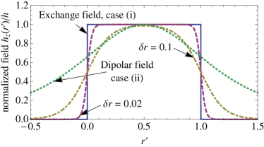
Figure 1: The dynamics in the different studies can be mapped on a time dependent field with amplitude $h_{z}(r^{\prime})$ (here normalized by its maximal value $h$) interacting with the spins positioned at integer sites. The discrete motion in the Ising/Potts model then corresponds to a step-function, which may be treated as a fixed spin interacting via exchange with one partner on the chain. The amplitude of a dipole field is sketched for comparison. The field used in this work may be tuned by adjusting the parameter $\delta r$ from one limiting case to the other.

For a certain time $1/v$ exactly one spin is exposed to the field with constant amplitude until the field reaches the next spin. Additionally the amplitude of the dipole field used in Fusco et al. (2008); Magiera et al. (2009, 2011); Magiera and Wolf (2010) is plotted. From Ref. Magiera et al. (2009) we know that for this case the adjustment of the spins with respect to the moved field happens in an adiabatic way, or in other words the time scale of relaxation is below that of the excitation. To generalize these setups, we consider a field with steepness $\delta r\ll 1$,

$$h_{z}(r^{\prime})=\frac{h}{\big{(}e^{-\frac{r^{\prime}}{\delta r}}+1\big{)}\big{(}e^{-\frac{1-r^{\prime}}{\delta r}}+1\big{)}},$$ (1)

which may be tuned from the step-like field ($\delta r=0$, now called limiting case (i)) to a slowly varying field ($\delta r\approx 0.1$, case (ii)). By shifting this field according to $r^{\prime}=r-vt$ we can directly influence the time scale at which the excitation at a fixed position $r$ occurs, $\tau_{\mathrm{switch}}\propto\delta r/v$.

We first consider a chain of classical, normalized Heisenberg spins ($|\mathbf{S}_{r}|{=}1$) of length $L$ with lattice spacing $a$, which interact with the field defined above. The corresponding time-dependent Hamiltonian is

$$\mathcal{H}(t)=-\sum_{r=1}^{L}J\;\mathbf{S}_{r}\cdot\mathbf{S}_{r+1}+d_{x}S_{r,x}^{2}+h_{z}(r-vt)S_{r,z},$$ (2)

with the exchange constant $J$. To get a well defined ground state, we use an easy axis anisotropy ($d_{x}{>}0$) and anti-periodic boundary conditions $\mathbf{S}_{r+L}{=}{-}\mathbf{S}_{r}$. The spins perform Landau-Lifshitz-Gilbert dynamics Landau and Lifshitz (1935); Gilbert (2004),

$$\frac{\mu_{s}(1+\alpha^{2})}{\gamma}\frac{\partial\mathbf{S}_{r}}{\partial t}=\mathbf{S}_{r}{\times}\frac{\partial\mathcal{H}}{\partial\mathbf{S}_{r}}+\alpha\mathbf{S}_{r}\times\left(\mathbf{S}_{r}{\times}\frac{\partial\mathcal{H}}{\partial\mathbf{S}_{r}}\right),$$ (3)

consisting of a precessional motion with a frequency proportional to $\gamma/\mu_{s}$, and a damping with the damping constant $\alpha$. For simplicity, we neglect temperature here, and the dynamic parameters yield a spin relaxation time $\tau_{\mathrm{rel}}$. The friction force $F$ can be either calculated from the dissipated power $P_{\mathrm{diss}}$ or the pumping power $P_{\mathrm{pump}}$, which are equal in the stationary state due to energy conservation and therefore we subsequently use $F=\left<P\right>/v$ after time averaging. The two cases can be described by

$$P(v)\propto v^{\phi},$$ (4)

with the dissipation exponent $\phi{=}1$ ($\phi{=}2$) for the Coulomb (Stokes) case. $P$ can be extracted from the energy terms by

$$P(t)=\frac{\partial\mathcal{H}}{\partial t}=\sum_{r=1}^{L}{\frac{\partial h_{z}(r-vt)}{\partial t}S_{r,z}}$$ (5)

which represents the power pumped into the system by the motion. In our simulations (c.f. Fig. 3a) we found $\phi{=}2$ for large $\tau_{\mathrm{switch}}$, which corresponds to the results in Fusco et al. (2008); Magiera et al. (2009, 2011); Magiera and Wolf (2010). For sufficiently small $\tau_{\mathrm{switch}}$ we get $\phi{=}1$, which was known from simulations in the Ising model, and was now reproduced in the Heisenberg model.

In the following we calculate the velocity $v_{\times}$ at which a cross-over from one regime to the other occurs. For case (i) only two spins contribute to the sum in Eq. (5) at the discrete times $vt\in\mathbb{Z}$ (at all other times and positions the field remains constant), and we can calculate the averaged pumping power by discretizing $\partial_{t}h_{z}$,

$$P_{\mathrm{C}}=-hv\left(\left<S_{1^{\prime},z}\right>-\left<S_{0^{\prime},z}\right>\right).$$ (6)

For the time $\tau_{\mathrm{ca}}$, corresponding to the time at which the amplitude of the field stays nearly constant, no pumping (respectively excitation) occurs. We consider $\tau_{\mathrm{ca}}{>}\tau_{\mathrm{rel}}$, i.e. the system always relaxes to equilibrium after a pumping event. Since the equilibrium configuration does not depend on the dynamics, Eq. 6 tells that here $\phi{=}1$. The equilibrium configuration for our choice of boundary conditions is a domain wall (DW) state, where the out-of-axis component is determined by the field and thus points in $z$-direction. As the field interacts mainly with only one spin, the shape of the DW is not influenced by $h$ and we may use the continuum limit profile ($a{\rightarrow}0$)

$$\mathbf{m}^{\mathrm{H}}(r^{\prime})=\left(\tanh{\left(r^{\prime}/\ell\right)},0,\mathrm{sech}{\left(r^{\prime}/\ell\right)}\right),$$ (7)

with the DW width $\ell{=}\sqrt{J/(2d_{x})}$, which can be calculated from minimizing the free energy Bulaevskii and Ginzburg (1964). By inserting $\langle\mathbf{S}_{0^{\prime}}\rangle{=}\mathbf{m}^{\mathrm{H}}(0)$ and $\langle\mathbf{S}_{1^{\prime}}\rangle{=}\mathbf{m}^{\mathrm{H}}(1)$ into Eq. (6) we now can calculate the power which is pumped into the system during each switching event. This quantity can be visualized in a potential plot. We again assume that $h$ does not influence the shape of the DW but its center $r_{\mathrm{dw}}$. As in limiting case (ii) the system is always near equilibrium, and in limiting case (i) it always reaches the ground state before being excited out of equilibrium, this assumption is justified and we can describe the whole configuration with $r_{\mathrm{dw}}$. We look at one cycle at which the field’s peak moves from $0$ to $1$, corresponding to the times $-1/2{\leq}vt{\leq}1/2$. For given $t$ we can calculate the system’s total energy as a function of $r_{\mathrm{dw}}$ (see the potential lines in Fig. 2). If the system evolved quasi statically, it would always be in the current potential minimum. In this picture $P_{\mathrm{C}}/v$ corresponds to the energy difference between the energy at $r_{\mathrm{dw}}{=}0,\,\,vt{=}{-}1/2$ (the equilibrium state) and $vt{=}1/2$ (the state which is present when the peak of the field has moved to the next spin while the DW is still at the same site). Results from simulations (plotted as squares in Fig. 2) confirm this: At $vt{=}0$ the system is excited to the upper state in a short time, and relaxes to the new ground state by adjusting $r_{\mathrm{dw}}$ slowly afterwards, until it reaches the new ground state configuration with $r_{\mathrm{dw}}{=}1$. Simulations of the second limiting case (circles in Fig. 2) confirm that the system is always near equilibrium, thus the DW slightly lags behind the ground state.

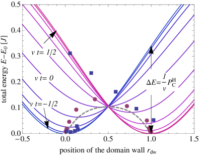
Figure 2: The system can be parameterized by the center of the DW $r_{\mathrm{dw}}$, thus for different times the total energy of the system can be calculated. This is done for field parameter $\delta r{=}0.1$ for 10 equidistant times (blue to purple curves). If the system evolved quasi static, it would follow the configuration of minimal energy, marked by the curve. Simulation results show both cases, the points indicate energy vs. $r_{\mathrm{dw}}$ for 10 time steps: (i) $\blacksquare$ The energy $P_{\mathrm{C}}^{\mathrm{H}}/v$ is periodically pumped into the system, which relaxes independent from $\tau_{\mathrm{switch}}$ afterwards. As the switching occurs at $vt=0$, we first see the relaxation from the preceding excitation in the left minimum, and at $vt=1/2$ the relaxation in the right minimum is not finished. (ii) $\bullet$ The system follows with a lag, but stays near equilibrium, slightly above the minimal energy configuration.

From our simulations, we found the pumping power

$$P_{\mathrm{S}}^{\mathrm{H}}=\frac{d_{x}\mu_{s}}{J\gamma\delta r}\alpha v^{2}.$$ (8)

The factor $d_{x}v/(\delta rJ)$ originates in the synchronization with the field, which changes at the time scale $\tau_{\mathrm{switch}}$. The factor $\alpha v\mu_{s}/\gamma$ emerges from spin dynamics, yielding a retardation of the DW as derived in Ref. Magiera et al. (2009). Setting

$$P_{\mathrm{C}}^{\mathrm{H}}(v)\stackrel{{\scriptstyle!}}{{=}}P_{\mathrm{S}}^{\mathrm{H}}(v):=P_{\times}^{\mathrm{H}}(v_{\times}^{\mathrm{H}})$$ (9)

yields the cross-over velocity

$$v^{\mathrm{H}}_{\times}=\frac{h\delta r}{\alpha d_{x}}\frac{\gamma J}{\mu_{s}}\left(1-\mathrm{sech}\left(1/\ell\right)\right),$$ (10)

where the system performs a cross-over from the Stokes-friction state to the Coulomb-friction state. In Fig. 3c these cross-over quantities have been calculated and the simulation results have been rescaled appropriately. The simulation data fit excellent over several magnitudes with the derived cross-over quantities, remaining deviations are discussed below.

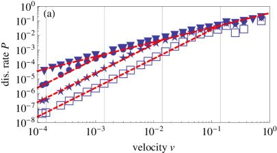
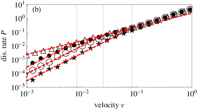
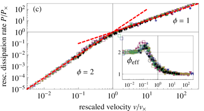
Figure 3: (Color online) Dissipated power vs. velocity (in natural units) for the a) Heisenberg ($d_{x}{=}0.5J,\alpha{=}0.5,h{=}J$, blue) and the b) Ising ($\beta{=}1/J,h{=}10J$, black) model. The simulated $\delta r$ are $\delta r{=}\infty$ ($\vartriangle$), $10^{-4}$ ($\blacktriangledown$), $10^{-3}$ (•), $3\times 10^{-3}(\circ)$, $10^{-2}$ (★) and $10^{-1}$ ($\square$). The grid lines mark the corresponding $v_{\times}$, the dashed lines display the calculated $P_{\mathrm{C}}(v)$ from Eq. (6) and fitted $P_{\mathrm{S}}(v)$. For c) we calculated explicitly the cross-over quantities $P_{\times}$ and $v_{\times}$ for both models from Eqs. (9,10), and plot the data again rescaled. Additionally we varied: $\alpha{=}0.3$ (purple), $h{=}2J$ (green) and $d_{x}{=}0.25J$ (yellow) for the same $\delta r$ set. In the inset we plot an effective exponent $\phi_{\mathrm{eff}}{=}\partial\log P/\partial\log v$, and get a universal cross-over from $2$ to $1$.

We performed also simulations of the isotropic Ising model with the same field and periodic boundary conditions ($S_{r+N}{=}S_{r}$). The Ising spins undergo spin flip dynamics with Metropolis probability Metropolis et al. (1953): Randomly chosen spins are flipped with the probability $p_{f}{=}\min{(1,\exp{(-\beta\Delta E)})}$, where $\beta$ is the inverse temperature and $\Delta E$ the energy difference between the flipped and the not flipped state.

For (i) we again find a behavior $\phi{=}1$. We assume that for (i) the spins relax after each switching event to the ground state profile which can be calculated via transfer matrix methods Hucht (2009):

$$m^{\mathrm{I}}(r^{\prime})=\tanh{(\beta h)}[\tanh{(\beta J)}]^{|r^{\prime}|}.$$ (11)

With $\langle S_{0^{\prime},z}\rangle{=}m^{\mathrm{I}}(0)$ and $\langle S_{1^{\prime},z}\rangle{=}m^{\mathrm{I}}(1)$ in Eq. (6), we get $P_{\mathrm{C}}^{I}$. $\phi{=}2$ is observed for (ii), and we fitted

$$P_{\mathrm{S}}^{\mathrm{I}}\propto v^{2}/\delta r.$$ (12)

We calculated again the cross-over velocity $v_{\times}^{\mathrm{I}}$, which is additionally plotted in Fig. 3b, and rescaled all data points for the cross-over plot, Fig. 3c.

Comparing Fig. 3a and Fig. 3b we come to the main result of our investigation, namely coincidence concerning the cross-over between both models, despite the substantial remaining differences like e.g. the dynamics of the models. The present deviations from the cross-over curve are discussed below. The slight increase of $P$, observed in the regime $v{>}0.1$ for all $\delta r$ in the Ising model is due to the fact that the system has not enough time to relax back to equilibrium before the next shift takes place and $m^{\mathrm{I}}(1)$ becomes significantly smaller than its equilibrium value. As the Heisenberg model contains spin wave excitations, we observed the generation of spin waves above a threshold velocity Magiera et al. (2011). In the cross-over plot these spin waves cause a kink above $v/v_{\times}{=}0.1$ for $\alpha{=}0.3$ (and a higher peak in the effective exponent plot). For very high velocities we observe a lowering of the power, which is due to a segregation of the peak of the field and the DW, leading to a reduced $m^{\mathrm{H}}_{z}(0){<}1$. This state with lowered dissipation has already been observed and reported in Ref. Magiera and Wolf (2010).

In conclusion, we presented a new model, which for the case of magnetic friction shows a transition from Stokes to Coulomb behavior, analogous to the Prandtl-Tomlinson model for solid friction. Whereas there, the elastic stiffness of the slider was the crucial parameter, it is the switching time of the magnetic field in our case. The comparison of both models sheds new light on the univeral origin of Coulomb behavior, which is based on a separation of the relaxation time from the much larger time scale on which the system gets excited. Our findings are in accordance to field theoretical results by Demery et al. Démery and Dean (2010, 2010), who also found Stokes-like friction as their system model does not contain discrete sites and thus $\tau_{\mathrm{ca}}=0$, i.e. the field is continiously driving the system. However, their simulation results are not correct as they simulated an Ising model with a discontinuous motion of a field, which is known to show Coulomb friction. This discrepancy stems from an incorrect definition of the friction force (Eq. (50) in Ref.Démery and Dean (2010), a correct definition has been presented in Kadau et al. (2008)).