Marginal density expansions for diffusions and stochastic volatility, part I: Theoretical Foundations

Abstract

Density expansions for hypoelliptic diffusions $\left(X^{1},\dots,X^{d}\right)$ are revisited. In particular, we are interested in density expansions of the projection $\left(X_{T}^{1},\dots,X_{T}^{l}\right)$, at time $T>0$, with $l\leq d$. Global conditions are found which replace the well-known ”not-in-cutlocus” condition known from heat-kernel asymptotics. Our small noise expansion allows for a ”second order” exponential factor. As application, new light is shed on the Takanobu–Watanabe expansion of Brownian motion and Lévy’s stochastic area. Further applications include tail and implied volatility asymptotics in some stochastic volatility models, discussed in the compagnion paper [14].

Keywords: Laplace method on Wiener space, generalized density expansions in small noise and small time, sub-Riemannian geometry with drift, focal points, Lévy’s stochastic area, Brownian motion on the Heistenberg group, stochastic volatility.

1 Introduction

Given a multi-dimensional hypoelliptic diffusion process $\mathrm{X}_{t}=\left(X_{t}^{1},\dots,X_{t}^{d}:t\geq 0\right)$, started at $\mathrm{X}_{0}=\mathrm{x}_{0}$, we are interested in the behaviour of the probability density function $f=f\left(\mathrm{y}\,,t\right)$ of the projected (in general non-Markovian) process

$$\mathrm{Y}_{t}:=\Pi_{l}\circ\mathrm{X}_{t}:=\left(X_{t}^{1},\dots,X_{t}^{l}\right),\,\,\,1\leq l\leq d\text{.}$$

Both short time asymptotics and tail asymptotics, in presence of some scaling, can be derived from the small noise problem

$$d\mathrm{X}_{t}^{\varepsilon}=b\left(\varepsilon,\mathrm{X}_{t}^{\varepsilon}\right)dt+\varepsilon\sigma\left(\mathrm{X}_{t}^{\varepsilon}\right)dW_{t},\quad\text{with }\mathrm{X}_{0}^{\varepsilon}=\mathrm{x}_{0}^{\varepsilon}\in\mathbb{R}^{d}.$$

Our main technical result, based on the Laplace method on Wiener space following Azencott, Bismut and, in particular, Ben Arous [3, 4] is a density expansion for $\mathrm{Y}_{t}^{\varepsilon}:=\Pi_{l}\circ\mathrm{X}_{t}^{\varepsilon}$ of the form, for $\mathrm{x}_{0},\mathrm{y},T$ fixed,

$$\text{ }f^{\varepsilon}\left(\mathrm{y},T\right)=e^{-c_{1}/\varepsilon^{2}}e^{c_{2}/\varepsilon}\varepsilon^{-l}\left(c_{0}+O\left(\varepsilon\right)\right)\text{ as }\varepsilon\downarrow 0.$$ (1)

Leaving definitions and precise statements to the main text below (cf theorem 8) let us briefly mention our key assumptions
(i) a strong Hörmander condition at all points (or in fact, a weak Hörmander condition at $\mathrm{x}_{0}$ and an explicit controllability condition);
(ii) existence of at most finitely many minimizers in the control problem which govern the leading order behaviour;
(iii) invertibility of the deterministic Malliavin covariance matrix at the minimizers;
(iv) a global condition on $\mathrm{x}_{0}\in\mathbb{R}^{d},\,\mathrm{y}\in\mathbb{R}^{l}$ which we call non-focality, motivated from terminology in Riemannian geometry.

Conditions (i)-(iii) will not surprise the reader familiar with the works [3, 4, 5, 45]. However, condition (iv) which guarantees non-degeneracy of the minimizers (cf. proposition 6), appears to be new in the context of density expansions, to the best of our knowledge, even in the elliptic case. It forms the essence of what is needed to extend the well-known point-point concept of non-conjugacy (crucial part of the ”$\notin$ cut-locus condition” familiar from heat kernel expansions) to a (sub-Riemannian, with drift) point-subspace setting. A simple (elliptic) example where (iv) and (1) fails, is given in section 4.3. A similar situation arises in the (hypoelliptic) example of Brownian motion and Lévy area, see section 4.4, where we recover (and then extend) some expansions previously derived by Takanobu–Watanabe [45]. We emphasize that our applications, notably those discussed in [14], require us to introduce and characterize non-focality in a control-theoretic generality; cf. section 3. (The reader may still be interested to consult geometry text books such as [9, 42] or [13, Section 4, p. 227-229] for more information on focality in the Riemannian setting.)

As far as the expansion (1) is concerned, we draw attention to the (in the context of density expansions) somewhat unusual second order exponential factor present when $c_{2}\neq 0$. As was understood in the context of the general Laplace method on Wiener space, [1, 2, 4], this has to do with allowing the drift vector field $b$ (and in the present paper also: the starting point) to depend on $\varepsilon$ at first order; the special case that arises from considering short time asymptotics - the small noise parameter $\varepsilon$ is then introduced by Brownian scaling - always leads to $c_{2}=0$. It is interesting to note that the work of Kusuoka–Stroock [33], concerning precise asymptotics for Wiener functionals (in the small noise limit), see also [38, 32] for recent applications to projected diffusions, was set up as an expansion in $\varepsilon^{2}$. This is enough to cover the model case of short time expansions, but cannot yield an expansion of the type (1) with $c_{2}\neq 0$. A similar remark applies to the small noise expansions for projected diffusions due to Takanobu–Watanabe [45].

Density expansions of diffusions in the small noise regime seem to go back (at least) to [30]; density expansions for projected diffusions in the small noise regime (which include the short time regime), with applications to implied volatility expansions, were recently considered by Y. Osajima [38], based on work with S. Kusuoka [32]. We partially improve on these results. First, as was already mentioned, $c_{2}=0$ in these works whereas expansions with $c_{2}\neq 0$ are crucial in understanding the tail behaviour of certain stochastic volatility models, [14] (see also [23, 17]). Additionally, in comparison with [38] we do not assume $x_{0}$ near $\left(y,\cdot\right)$, nor ellipticity of the problem. In further contrast to (the general results in) [32, 33] we provide a checkable, finite-dimensional criterion that guarantees that the crucial infinite-dimensional non-degeneracy assumption, left as such in [32, 33], is actually satisfied. On the other hand, these authors give somewhat explicit formulae for $c_{0}$ which we (presently) do not.

Finally, our expansion (1) leads to short time expansion for projected diffusion densities, under global conditions on $\left(\mathrm{x}_{0},\mathrm{y}\right)$, of the form

$$f\left(\mathrm{y},t\right)\sim c_{0}\left(\mathrm{x}_{0},\mathrm{y}\right)\frac{1}{t^{l/2}}\exp\left(-\frac{d^{2}\left(\mathrm{x}_{0},\mathrm{y}\right)}{2t}\right)\text{ as }t\downarrow 0.$$ (2)

When $l=d$, such expansions go back to classical works ranging from Molchanov [35] to Ben Arous [3]. The leading order behaviour $2t\log f\left(\mathrm{y},t\right)\sim-d^{2}\left(\mathrm{x}_{0},\mathrm{y}\right)$ is due to Varadhan [46]. The case $l<d$, in particular our global condition on $\left(\mathrm{x}_{0},\mathrm{y}\right)$, appears to be new. That said, expansions of this form have appeared in [45, 26, 38]; the last two references aimed at implied volatility expansions. In the context of time homogenous local volatility models ($l=d=1$), the expansion (2) holds trivially without any conditions on $\left(\mathrm{x}_{0},\mathrm{y}\right)$; the resulting expansion was derived (with explicit constant $c_{0}$) in [21]. Subject to mild technical conditions on the diffusion coefficient, they show how to deduce first a call price and then an implied volatility expansion in the short time (to maturity) regime

$$\sigma_{BS}\left(k,t\right)=|k|/d\left(\mathrm{x}_{0},k\right)+c\left(\mathrm{x}_{0},k\right)t+O\left(t^{2}\right)\text{ as }t\downarrow 0;$$

where $d\left(\mathrm{x}_{0},k\right)$ is a point-point distance and $c\left(\mathrm{x}_{0},k\right)$ is explicitly given; $k$ is $\log$-strike (better: log-forward in moneyness). The celebrated Berestycki–Busca–Florent (BBF) formula [10] asserts that $\sigma_{BS}\left(k,t\right)\sim|k|/d\left(\mathrm{x}_{0},k\right)$ as $t\downarrow 0$, and is in fact valid in generic stochastic volatility models, $d\left(\mathrm{x}_{0},k\right)$ is then understood as a point-hyperplane distance. In fact, $|k|/d\left(\mathrm{x}_{0},k\right)$ arose as the initial condition of a non-linear evolution equation for the entire implied volatility surface. As briefly indicated in [10, Sec 6.3] this can be used for a Taylor expansion of $\sigma_{BS}\left(k,t\right)$ in $t$. Such expansions have also been discussed, based on heat kernel expansions on Riemannian manifolds by [12, 27, 39], not always in full mathematical rigor. Some mathematical results are given in [38], assuming ellipticity and close-to-the-moneyness $\left|k\right|<<1$; see also forthcoming work by Ben Arous–Laurence [8]. We suspect that our formula (2), potentially applicable far-from-the-money, will prove useful in this context and shall return to this in future work.

It should be noted that the BBF formula alone can be obtained from soft large deviation arguments, cf. [40, Sec. 3.2.1] and the references therein. In a similar spirit, cf. [47, Sec 5, Rmk 2.9], the Varadhan-type formula $2t\log f\left(\mathrm{y},t\right)\sim-d^{2}\left(\mathrm{x}_{0},\mathrm{y}\right)$, when $l<d$, can be shown, without any conditions on $(\mathrm{x}_{0},\mathrm{y})$ by large deviation methods, only relying on the existence of a reasonable density.

As a final note, we recall that the (in general, non-Markovian) $\mathbb{R}^{l}$-valued Itô-process $\left(\mathrm{Y}_{t}:t\geq 0\right)$ admits - subject to some technical assumptions [24, 41] - a Markovian (or Gyöngy) projection. That is, a time-inhomogeneous Markov diffusion $(\mathrm{\tilde{Y}}_{t}:t\geq 0)$ with matching time-marginals i.e $\mathrm{Y}_{t}=\mathrm{\tilde{Y}}_{t}$  (in law) for every fixed $t\geq 0$. In a financial context, when $l=1$, this process is known as the (Dupire) local volatility model and various authors [10, 12, 27, 8] have used this as an important intermediate step in computing implied volatility in stochastic volatility models. Since all our expansions (small noise, tail, short time ) are relative to such time-marginals they may also be viewed as expansions for the corresponding Markovian projections.

Acknowledgement: JDD and AJ acknowledge (partial resp. full) financial support from MATHEON. PKF acknowledges partial support from MATHEON and the European Research Council under the European Union’s Seventh Framework Programme (FP7/2007-2013) / ERC grant agreement nr. 258237. PKF would like to thank G. Ben Arous for pointing out conceptual similarities in [17, 3] and several discussions thereafter. It is also a pleasure to thank F. Baudoin, J.P. Gauthier, A. Gulisashvili and P. Laurence for their interest and feedback.

2 The main result and its corollaries

Consider a $d$-dimensional diffusion $\left(\mathrm{X}_{t}^{\varepsilon}\right)_{t\geq 0}$ given by the stochastic differential equation

$$d\mathrm{X}_{t}^{\varepsilon}=b\left(\varepsilon,\mathrm{X}_{t}^{\varepsilon}\right)dt+\varepsilon\sigma\left(\mathrm{X}_{t}^{\varepsilon}\right)dW_{t},\quad\text{with }\mathrm{X}_{0}^{\varepsilon}=\mathrm{x}_{0}^{\varepsilon}\in\mathbb{R}^{d}$$ (3)

and where $W=(W^{1},\dots,W^{m}$) is an $m$-dimensional Brownian motion. Unless otherwise stated, we assume $b:[0,1)\times\mathbb{R}^{d}\rightarrow\mathbb{R}^{d},$ $\sigma=\left(\sigma_{1},\dots,\sigma_{m}\right):\mathbb{R}^{d}\rightarrow\mathrm{Lin}\left(\mathbb{R}^{m}\rightarrow\mathbb{R}^{d}\right)$ and $\mathrm{x}_{0}^{\cdot}:[0,1)\rightarrow\mathbb{R}^{d}$ to be smooth, bounded with bounded derivatives of all orders. Set $\sigma_{0}=b\left(0,\cdot\right)$ and assume that, for every multiindex $\alpha$, the drift vector fields $\left\{b\left(\varepsilon,\cdot\right):\varepsilon>0\right\}$ converge to $\sigma_{0}$ in the sense

$$\partial_{x}^{\alpha}b\left(\varepsilon,\cdot\right)\rightarrow\partial_{x}^{\alpha}b\left(0,\cdot\right)=\partial_{x}^{\alpha}\sigma_{0}\left(\cdot\right)\text{ uniformly on compacts as }\varepsilon\downarrow 0\text{.}$$ (4)

We shall also assume that

$$\partial_{\varepsilon}b\left(\varepsilon,\cdot\right)\rightarrow\partial_{\varepsilon}b\left(0,\cdot\right)\text{ \ uniformly on compacts as }\varepsilon\downarrow 0$$ (5)

and (one-sided) differentiability of the starting point in $\varepsilon$,

$$\mathrm{x}_{0}^{\varepsilon}=\mathrm{x}_{0}+\varepsilon\mathrm{\hat{x}}_{0}+o\left(\varepsilon\right)\text{ as }\varepsilon\downarrow 0\text{. }$$ (6)

Leaving applications to stochastic volatility models to [14], the main result of this paper is a density expansion in $\varepsilon$ of the $\mathbb{R}^{l}$-valued projection

$$\mathrm{Y}_{T}^{\varepsilon}:=\Pi_{l}\circ\mathrm{X}_{T}^{\varepsilon}:=\left(X_{T}^{\varepsilon,1},\dots,X_{T}^{\varepsilon,l}\right)\in\mathbb{R}^{l};$$

where $\Pi_{l}$ denotes the projection $\left(x^{1},\dots,x^{d}\right)\mapsto\left(x^{1},\dots,x^{l}\right)$, for fixed $l\in\left\{1,\dots,d\right\}$ and $T>0$. Of course, we need to guarantee that $\mathrm{Y}_{T}^{\varepsilon}$ indeed admits a density. We make the standing assumption that the weak Hörmander condition holds at $\mathrm{x}_{0}$,

$$\text{{span}}\left[\sigma_{i}:1\leq i\leq m;\text{ }\left[\sigma_{j},\sigma_{k}\right]:0\leq j,k\leq m;...\right]_{\mathrm{x}_{0}}=\mathcal{T}_{\mathrm{x}_{0}}\mathbb{R}^{d};$$ (H)

that is, the linear span of $\sigma_{1},\dots,\sigma_{m}$ and all Lie brackets of $\sigma_{0},\sigma_{1},\dots,\sigma_{m}$ at the starting point is full. Since this condition is ”open” it also holds, thanks to (4), for $\varepsilon>0$ small enough, with $\sigma_{0}$ and $\mathrm{x}_{0}$ replaced by ${b}\left(\varepsilon,\cdot\right)$ (or $\tilde{b}\left(\varepsilon,\cdot\right)$, cf. previous footnote) and $\mathrm{x}_{0}^{\varepsilon}$, respectively. It then is a classical result (due to Hörmander, Malliavin; see e.g. [37]) that the $\mathbb{R}^{d}$-valued r.v. $\mathrm{X}_{T}^{\varepsilon}$ admits a (smooth) density for all times $T>0$ and so does its $\mathbb{R}^{l}$-valued projection $\mathrm{Y}_{T}^{\varepsilon}$. We denote the probability density of $\mathrm{Y}_{T}^{\varepsilon}$ by $f^{\varepsilon}\left(\cdot,T\right)\equiv f^{\varepsilon}\left(\mathrm{y},T\right)$ with $\mathrm{y}\in\mathbb{R}^{l}$. In theorem 8 below, where we expand

$$f^{\varepsilon}\left(\mathrm{y},T\right)|_{\mathrm{y}=\mathrm{a}}=f^{\varepsilon}\left(\mathrm{a},T\right)$$

in $\varepsilon$ for some fixed $\mathrm{a}\in\mathbb{R}^{l}$, a crucial assumption is that $\mathcal{K}_{\mathrm{a}}$, defined by

$$\mathcal{K}_{\mathrm{x}_{0},T;\mathrm{a}}=\mathcal{K}_{\mathrm{a}}:=\left\{\mathrm{h}\in H:\Pi_{l}\circ\phi_{T}\left(h\right)=\mathrm{a}\right\},$$ (7)

is non-empty. Here, $H$ denotes the Cameron-Martin space, i.e. absolutely continuous paths with derivative in $L^{2}\left(\left[0,T\right],\mathbb{R}^{m}\right)$, with norm given by

$$\left\|\mathrm{h}\right\|_{H}^{2}=\sum_{i=1}^{m}\int_{0}^{T}|\dot{h}_{t}^{i}|^{2}dt,\,\,\,\,\,\,\,\forall\mathrm{h}=\left(h^{1},\dots,h^{m}\right)\in H.$$

We write $\phi_{T}\left(\mathrm{h}\right)$ for the time-$T$ solution to the controlled ordinary differential equation (e.g. [19, Sec.3])

$$d\phi_{t}^{\mathrm{h}}=\sigma_{0}\left(\phi_{t}^{\mathrm{h}}\right)dt+\sum_{i=1}^{m}\sigma_{i}\left(\phi_{t}^{\mathrm{h}}\right)dh_{t}^{i},\,\,\phi_{0}^{\mathrm{h}}=\mathrm{x}_{0}\in\mathbb{R}^{d}.$$ (8)

At occasions, we emphasize the starting point $\mathrm{x}_{0}$ by writing $\phi_{T}^{\mathrm{h}}\left(\mathrm{x}_{0}\right)$, and note that $\phi_{T}\left(\mathrm{h}\right)=\phi_{T}^{\mathrm{h}}\left(\mathrm{\cdot}\right)$, i.e. the mappig $\mathrm{x}_{0}\in\mathbb{R}^{d}\mapsto$ $\phi_{T}^{\mathrm{h}}\left(\mathrm{x}_{0}\right)\in\mathbb{R}^{d}$, is a diffeomorphism. Similarly, we write $\phi_{T\leftarrow t}\left(\mathrm{h}\right)$ for the time-$T$ solution, but started at time $t$. Each such $\phi_{T\leftarrow t}\left(\mathrm{h}\right)$ is again a diffeomorphism, and we denote its differential by $\Phi_{T\leftarrow t}\left(\mathrm{h}\right)$. A well-known sufficient condition for $\mathcal{K}_{\mathrm{a}}\neq\varnothing$  is the strong Hörmander condition (at all points)

$$\forall\mathrm{x}\in\mathbb{R}^{d}:\text{{Lie}}\left[\sigma_{1},\dots,\sigma_{m}\right]|_{\mathrm{x}}=\mathcal{T}_{\mathrm{x}}\mathbb{R}^{d}\cong\mathbb{R}^{d};$$ (H1)

see [29, p.106] or [25, p.441],[31] for instance.

Whenever $\mathcal{K}_{\mathrm{a}}\neq\varnothing$, it makes sense to define the energy and the set of minimizers

$$\Lambda_{\mathrm{x}_{0},T}\left(\mathrm{a}\right) : =\Lambda\left(\mathrm{a}\right):=\inf\left\{\frac{1}{2}\|\mathrm{h}\|_{H}^{2}:\mathrm{h}\in\mathcal{K}_{\mathrm{a}}\right\},$$ (9)

$$\mathcal{K}_{\mathrm{a}}^{\min} : =\left\{\mathrm{h}_{0}\in\mathcal{K}_{\mathrm{a}}:\frac{1}{2}\|\mathrm{h}_{0}\|_{H}^{2}=\Lambda\left(\mathrm{a}\right)\right\}.$$

In words, $\Lambda\left(\mathrm{a}\right)$ is the minimal energy required to go in time $T$ from $\mathrm{x}_{0}\in\mathbb{R}^{d}$ to the ”target” submanifold

$$N:=N_{\mathrm{a}}:=\left\{\mathrm{x}\in\mathbb{R}^{d}:\Pi_{l}\left(\mathrm{x}\right)=\left(x^{1},\dots,x^{l}\right)=\mathrm{a}\right\}.$$

Elements of $\mathcal{K}_{\mathrm{a}}^{\min}$ will be called minimizers or minimizing controls. A standard weak-compactness argument (e.g. [11, Thm 1.14]) shows that $\mathcal{K}_{\mathrm{a}}\neq\varnothing$ already implies that $\mathcal{K}_{\mathrm{a}}^{\min}$ is non-empty. (Throughout the paper, we shall only be concerned with the situation that $\mathcal{K}_{\mathrm{a}}^{\min}$ contains one or finitely many minimizers.)

It will be crucial that $\mathcal{K}_{\mathrm{a}}$ enjoys a (Hilbert) manifold structure, locally around (each) $\mathrm{h}_{0}\in\mathcal{K}_{\mathrm{a}}^{\min}$ . Following Bismut [11, Thm 1.5] this can be guaranteed by assuming invertibility of $C_{\mathrm{x}_{0},T;\mathrm{a}}\left(\mathrm{h}_{0}\right)$, the deterministic Malliavin matrix given by

$$C_{\mathrm{x}_{0},T;\mathrm{a}}\left(\mathrm{h}\right):=C\left(\mathrm{h}\right):=\left\langle D\phi_{T}\left(\mathrm{h}\right),D\phi_{T}\left(\mathrm{h}\right)\right\rangle_{H}\in\mathrm{Lin}\left(\mathcal{T}_{\mathrm{x}_{T}}^{\ast}\mathbb{R}^{d}\rightarrow\mathcal{T}_{\mathrm{x}_{T}}\mathbb{R}^{d}\right)\cong\mathbb{R}^{d\times d}$$

where $\mathrm{x}_{T}:=\phi_{T}\left(\mathrm{h}\right)$ and $D$ will always denote the ($H$-valued) Fréchet derivative of some function depending on $\mathrm{h}\in H$. We can also view $C\left(\mathrm{h}\right)$ as (positive semi-definite) quadratic form on $\mathcal{T}_{\mathrm{x}_{T}}^{\ast}\mathbb{R}^{d}$, in coordinates, with $\mathrm{p}=p_{i}dx^{i}\in\mathcal{T}_{\mathrm{x}_{T}}^{\ast}\mathbb{R}^{d}$,

$$\left\langle C\left(\mathrm{h}\right)\mathrm{p},\mathrm{p}\right\rangle=\left\|\left\langle\mathrm{p},D\phi_{T}\left(\mathrm{h}\right)\right\rangle\right\|_{H}^{2}=\left\|\sum_{i=1}^{d}p_{i}D\phi_{T}^{i}\left(\mathrm{h}\right)\right\|_{H}^{2}\text{ . }$$

In fact, large parts of our analysis only rely on non-degeneracy of $C\left(\mathrm{h}_{0}\right)$ restricted to $\mathbb{R}^{l\times l}$ but we find it more convenient to deal with the ”full” matrix $C\left(\mathrm{h}_{0}\right)$. A sufficient condition for ”$C\left(\mathrm{h}\right)$ is invertible for every $\mathrm{h}\neq 0$” in a strictly sub-elliptic setting is given as condition (H2) by [11]; although much stronger than Hörmander’s condition, it does apply to examples such as the $3$-dimensional Heisenberg group and thus Lévy’s area, cf. section 4.4. Most financial applications, as discussed in [14], are actually locally elliptic, or ”almost elliptic”, and are covered by the following condition.

Proposition 1

Assume $\mathrm{h}\in H$ and the condition

$$\exists t\in\left[0,T\right]:\mathrm{span}\left[\sigma_{1},\dots,\sigma_{m}\right]|_{\mathrm{x}_{t}}=\mathcal{T}_{\mathrm{x}_{t}}\mathbb{R}^{d}$$

where $\mathrm{x}_{t}:=\phi_{t}\left(\mathrm{h}\right)$. Then $C\left(\mathrm{h}\right)$ is invertible.

Proof. We have the well-known formula (e.g. [45, (4.1)]), for any $\,\mathrm{k}=\left(k^{1},\dots,k^{m}\right)\in H,$

$$\left\langle D\phi_{T}\left(\mathrm{h}\right),\mathrm{k}\right\rangle_{H}=D\phi_{T}\left(\mathrm{h}\right)\left[\mathrm{k}\right]=\int_{0}^{T}\sum_{j=1}^{m}\Phi_{T\leftarrow t}\left(\mathrm{h}\right)\sigma_{j}\left(\mathrm{x}_{t}\right)\dot{k}_{t}^{j}dt\in\mathcal{T}_{\mathrm{x}_{T}}\mathbb{R}^{d}\,\,$$

When pairing this with $\mathrm{p}=p_{i}dx^{i}\in\mathcal{T}_{\mathrm{x}_{T}}^{\ast}\mathbb{R}^{d}$, we have

$$\left\langle\left\langle\mathrm{p},D\phi_{T}\left(\mathrm{h}\right)\right\rangle,\mathrm{k}\right\rangle_{H}=\int_{0}^{T}\sum_{j=1}^{m}\left\langle\mathrm{p},\Phi_{T\leftarrow t}\left(\mathrm{h}\right)\sigma_{j}\left(\mathrm{x}_{t}\right)\right\rangle\dot{k}_{t}^{j}dt\in\mathcal{T}_{\mathrm{x}_{T}}\mathbb{R}^{d}$$

and it easily follows that $\left\langle C\left(\mathrm{h}\right)\mathrm{p},\mathrm{p}\right\rangle$ is given by

$$\left\|\left\langle\mathrm{p},D\phi_{T}\left(\mathrm{h}\right)\right\rangle\right\|_{H}^{2}=\int_{0}^{T}\sum_{j=1}^{m}\left\langle\mathrm{p},\Phi_{T\leftarrow t}\left(\mathrm{h}\right)\sigma_{j}\left(\mathrm{x}_{t}\right)\right\rangle^{2}dt=\int_{0}^{T}\sum_{j=1}^{m}\left\langle\left(\Phi_{T\leftarrow t}\left(\mathrm{h}\right)\right)^{\ast}\mathrm{p},\sigma_{j}\left(\mathrm{x}_{t}\right)\right\rangle^{2}dt.$$

Assume now $\left\langle C\left(\mathrm{h}\right)\mathrm{p},\mathrm{p}\right\rangle=0$. By assumption span$\left[\sigma_{1},\dots,\sigma_{m}\right]|_{\mathrm{x}_{t}}=\mathcal{T}_{\mathrm{x}_{t}}\mathbb{R}^{d}$ for some $t\in\left[0,T\right]$, and this clearly remains valid in a small enough open interval containing $t$ which is enough to conclude $\left(\Phi_{T\leftarrow t}\left(\mathrm{h}\right)\right)^{\ast}\mathrm{p}\equiv 0$. By non-degeneracy of the (co-)tangent flow, this implies $\mathrm{p}=0$ and so $C\left(\mathrm{h}\right)$ is non-degenerate, as claimed.   

We now introduce the Hamiltonian

$$\mathcal{H}\left(\mathrm{x},\mathrm{p}\right) : =\left\langle\mathrm{p},\sigma_{0}\left(\mathrm{x}\right)\right\rangle+\frac{1}{2}\sum_{i=1}^{m}\left\langle\mathrm{p},\sigma_{i}\left(\mathrm{x}\right)\right\rangle^{2}$$

$$= \left\langle\mathrm{p},\sigma_{0}\left(\mathrm{x}\right)\right\rangle+\frac{1}{2}\left\langle\mathrm{p},\left(\sigma\sigma^{T}\right)\left(\mathrm{x}\right)\mathrm{p}\right\rangle$$

and H${}_{t\leftarrow 0}=$H${}_{t\leftarrow 0}\left(\mathrm{x}_{0},\mathrm{p}_{0}\right)$ as the flow associated to the vector field $\left(\partial_{\mathrm{p}}\mathcal{H},-\partial_{\mathrm{x}}\mathcal{H}\right)$ on $\mathcal{T}^{\ast}\mathbb{R}^{d}$. (As in [11, p.37], this vector field is complete, i.e. H_⋅←0 does not explode.)

The following propositions generalize the respective results in Bismut’s book [11] (see also Ben Arous [3, Theorems 1.15 and 1.1.8]) from a drift-free ($\sigma_{0}\equiv 0$), point-to-point setting ($\mathrm{x}_{0}\in\mathbb{R}^{d}$ to $\mathrm{y}\in\mathbb{R}^{d}$) to a point-to-subspace setting ($\mathrm{x}_{0}\in\mathbb{R}^{d}$ to $\left(\mathrm{y},\cdot\right)\in\mathbb{R}^{l}\oplus\mathbb{R}^{d-l}$) with non-zero drift vector field $\sigma_{0}$. Note that the Bismut setting [11, Chapter I] is recovered by taking zero drift, $\sigma_{0}\equiv 0$, and $l=d$.

Proposition 2

If (i) $\mathrm{h}_{0}\in\mathcal{K}_{\mathrm{a}}^{\min}$ is a minimizing control and (ii) the deterministic Malliavin covariance matrix $C\left(\mathrm{h}_{0}\right)$ is invertible then there exists a unique $\mathrm{p}_{0}=\mathrm{p}_{0}\left(\mathrm{h}_{0}\right)\in\mathcal{T}_{\mathrm{x}_{0}}^{\ast}\mathbb{R}^{d}$, in fact

$$\mathrm{p}_{0}\in\left(\Phi_{T\leftarrow 0}\left(\mathrm{h}_{0}\right)\right)^{\ast}\mathrm{span}\left\{dx^{1},\dots,dx^{l}\right\}|_{\phi_{T}^{h}\left(\mathrm{x}_{0}\right)},$$

such that

$$\phi_{t}^{\mathrm{h}_{0}}\left(\mathrm{x}_{0}\right)=\pi\mathrm{H}_{t\leftarrow 0}\left(\mathrm{x}_{0}\mathrm{,p}_{0}\right),\text{ }0\leq t\leq T$$ (10)

($\pi$ denotes the projection from $\mathcal{T}^{\ast}\mathbb{R}^{d}$ onto $\mathbb{R}^{d}$; in coordinates $\pi\left(\mathrm{x},\mathrm{p}\right)=\mathrm{x}$)
Moreover, $\left(\mathrm{x}\left(t\right),\mathrm{p}\left(t\right)\right):=\mathrm{H}_{t\leftarrow 0}\left(\mathrm{x}_{0},\mathrm{p}_{0}\right)$ solves the Hamiltonian ODEs in $\mathcal{T}^{\ast}\mathbb{R}^{d}\cong\mathbb{R}^{d}\oplus\mathbb{R}^{d}$

$$\left(\begin{array}[]{c}\mathrm{\dot{x}}\\ \mathrm{\dot{p}}\end{array}\right)=\left(\begin{array}[]{c}\partial_{\mathrm{p}}\mathcal{H}\left(\mathrm{x}\left(t\right),\mathrm{p}\left(t\right)\right)\\ -\partial_{\mathrm{x}}\mathcal{H}\left(\mathrm{x}\left(t\right),\mathrm{p}\left(t\right)\right)\end{array}\right),$$ (11)

the minimizing control $\mathrm{h}_{0}=\mathrm{h}_{0}\left(\cdot\right)$ is recovered by

$$\mathrm{\dot{h}}_{0}=\left(\begin{array}[]{c}\,\left\langle\sigma_{1}\left(\mathrm{x}\left(\cdot\right)\right),\mathrm{p}\left(\cdot\right)\right\rangle\\ \dots\\ \,\,\left\langle\sigma_{m}\left(\mathrm{x}\left(\cdot\right)\right),\mathrm{p}\left(\cdot\right)\right\rangle\end{array}\right).$$ (12)

At last, crucial for actual computations, $\left(\mathrm{x}\left(t\right),\mathrm{p}\left(t\right)\right)=\mathrm{H}_{t\leftarrow 0}\left(\mathrm{x}_{0},\mathrm{p}_{0}\right)$ satisfies the Hamiltonian ODEs (11) as boundary value problem, subject to the following initial -, terminal - and transversality conditions,

$$\mathrm{x}\left(0\right) = \mathrm{x}_{0}\in\mathbb{R}^{d},$$

$$\mathrm{x}\left(T\right) = \left(\mathrm{a},\cdot\right)\in\mathbb{R}^{l}\mathbb{\oplus R}^{d-l}\cong\mathbb{R}^{d},$$

$$\mathrm{p}\left(T\right) = \left(\cdot,0\right)\in\mathbb{R}^{l}\mathbb{\oplus R}^{d-l}\cong\mathcal{T}_{\mathrm{x}\left(T\right)}^{\ast}\mathbb{R}^{d}.$$ (13)

Remark 3

With $C:=\mathcal{H}\left(\mathrm{x}\left(t\right),\mathrm{p}\left(t\right)\right)$ independent of $t\in\left[0,T\right]$, one has

$$\Lambda\left(\mathrm{a}\right)=\frac{1}{2}\|\mathrm{h}_{0}\|_{H}^{2}=TC-\frac{1}{2}\int_{0}^{T}\left\langle\sigma_{0}\left(\mathrm{x}\left(t\right)\right),\mathrm{p}\left(t\right)\right\rangle dt\text{.}$$ (14)

Proof. The key remark, due to Bismut [11, Chapter I], is that under the assumption ”$\exists C\left(\mathrm{h}_{0}\right)^{-1}$” the set $\mathcal{K}_{\mathrm{a}}^{\min}$ can be described by Hamilton–Jacobi theory. It then suffices to adapt the arguments of Bismut, as done in the drift-free case by Takanobu–Watanabe, [45, Prop. 4.1]. Let us note that the additional drift vector field $\sigma_{0}$ is trivially incorporated in their setting, cf. the evolution given in (8), by adding a $0$th component to the controls, i.e. $h_{t}^{0}\equiv t$. The boundary conditions - in particular, transversality, have not been pointed out explicitly in [45] although are implicitly contained in their formulation. In fact, formal application of Pontryagin’s maximum principle leads precisely to the above boundary value problem; care is necessary, however, since without assuming invertibility of $C\left(\mathrm{h}_{0}\right)$, one can be in the so-called ”strictly abnormal” case; the above approach is then not possible.   

Remark 4

Assume that $\mathrm{y}\mapsto\mathrm{h}_{0}\left(\mathrm{y}\right)\in\mathcal{K}_{\mathrm{y}}^{\min}$ is a smooth map (in a neighbourhood of the fixed point $\mathrm{a}$). Writing ^′ for the derivative with respect to ${\mathrm{y}}$, we have

$$\Lambda\left(\mathrm{y}\right)=\frac{1}{2}\left\|\mathrm{h}_{0}\left(\mathrm{y}\right)\right\|^{2}\implies\Lambda^{\prime}\left(\mathrm{a}\right)=\left\langle\mathrm{h}_{0}\left(\mathrm{a}\right),\mathrm{h}^{\prime}_{0}\left(\mathrm{a}\right)\right\rangle_{H}.$$

On the other hand, it follows from $\Pi_{l}\phi_{T}\left(\mathrm{h}_{0}\left(\mathrm{y}\right)\right)=\mathrm{y}$ that

$$\left(\Pi_{l}\right)_{\ast}D\phi_{T}\left(\mathrm{h}_{0}\left(\mathrm{a}\right)\right)\left[\mathrm{h}^{\prime}_{0}\left(\mathrm{a}\right)\right]=\mathrm{Id}\text{ on }\mathbb{R}^{l}.$$ (15)

Write $\mathrm{p}\left(T\right)=\left(\mathrm{q}\left(\mathrm{a}\right),0\right)\in\left(\cdot,0\right)$ as determined by the previous proposition, equation (13), where our notation $\mathrm{q}=\mathrm{q}\left(\mathrm{a}\right)$ emphasizes the dependency on $\mathrm{a}$, with $T$ fixed. One has (cf. lemma 14)

$$\mathrm{h}_{0}\left(\mathrm{a}\right)=D\phi_{T}\left(\mathrm{h}_{0}\left(\mathrm{a}\right)\right)^{\ast}\mathrm{p}\left(T\right)=\left(\left(\Pi_{l}\right)_{\ast}D\phi_{T}\left(\mathrm{h}_{0}\left(\mathrm{a}\right)\right)\right)^{\ast}\mathrm{q}\left(\mathrm{a}\right)$$

and it follows that

$$\Lambda^{\prime}\left(\mathrm{a}\right)=\left\langle\mathrm{h}_{0}\left(\mathrm{a}\right),\mathrm{h}^{\prime}_{0}\left(\mathrm{a}\right)\right\rangle_{H}=\left\langle\mathrm{q}\left(\mathrm{a}\right),\left(\Pi_{l}\right)_{\ast}D\phi_{T}\left(\mathrm{h}_{0}\left(\mathrm{y}\right)\right)\mathrm{h}^{\prime}_{0}\left(\mathrm{a}\right)\right\rangle.$$

Thanks to (15) we now see that

$$\Lambda^{\prime}\left(\mathrm{a}\right)=\mathrm{q}\left(\mathrm{a}\right).$$ (16)

This can be a useful short-cut when computing the energy from the Hamiltonian system. If $\#\mathcal{K}_{\mathrm{a}}^{\min}=1$ for some $\mathrm{a}$, and our non-degeneracy condition (ND) as introduced below is met, the existence of such a map $\mathrm{h}_{0}\left(\mathrm{\cdot}\right)$ can be shown along the lines of [11, Thm 1.26]. We shall not rely on formula (16) in the sequel.

Remark 5 (How to compute optimal controls $h_{0}$)

Proposition 2 - as it stands - requires $\mathrm{h}_{0}$ to be a minimizer and then, subject to condition (ii), provides us with some information about $\phi^{\mathrm{h}_{0}}\left(\mathrm{x}_{0}\right)$ and in particular allows us to reconstruct $\mathrm{h}_{0}$ from the Hamiltonian flow

$$\left(\mathrm{x,p}\right)\equiv H_{\cdot\leftarrow 0}\left(\mathrm{x}_{0},\mathrm{p}_{0}\right)=H_{\cdot\leftarrow T}\left(\mathrm{x}_{T},\mathrm{p}_{T}\right),$$

cf. equation (12). That said, we can consider any solution to the boundary valued problem (11),(13), say $\left(\mathrm{\hat{x}},\mathrm{\hat{p}}\right)$, and define a (possibly non-minimizing) control path ĥ₀ via (12) i.e.

$$\mathrm{\hat{h}}_{0}^{i}=\int_{0}^{\cdot}\,\left\langle\sigma_{i}\left(\mathrm{\hat{x}}\left(t\right)\right),\mathrm{\hat{p}}\left(t\right)\right\rangle dt,\,\,\,\,i=1,\dots,m.$$

From (11),

$$d\mathrm{\hat{x}}_{t}=\partial_{\mathrm{p}}\mathcal{H}\left(\mathrm{\hat{x}}_{t},\mathrm{\hat{p}}_{t}\right)dt=\sigma_{0}\left(\mathrm{\hat{x}}_{t}\right)dt+\sum_{i=1}^{m}\sigma_{i}\left(\mathrm{\hat{x}}_{t}\right)\left\langle\sigma_{i}\left(\mathrm{\hat{x}}_{t}\right),\mathrm{\hat{p}}_{t}\right\rangle dt$$

and so relation (10) remains valid i.e. $\phi_{t}^{\mathrm{\hat{h}}_{0}}\left(\mathrm{x}_{0}\right)=\mathrm{\hat{x}}_{t}$. It follows that the boundary conditions valid for x̂ (namely, x̂$\left(0\right)=\mathrm{x}_{0},\Pi_{l}$x̂$\left(T\right)=\mathrm{a}$) are also valid for $\phi^{\mathrm{\hat{h}}_{0}}\left(\mathrm{x}_{0}\right)$ and hence $\mathrm{\hat{h}}_{0}$ $\in\mathcal{K}_{\mathrm{a}}$. While we do not know if $\mathrm{\hat{h}}_{0}\in\mathcal{K}_{\mathrm{a}}^{\min}$, proposition 2 guarantees that every minimizer $\mathrm{h}_{0}$ $\in\mathcal{K}_{\mathrm{a}}^{\min}$ can be found be the above procedure. We thus have the following recipe:
(i) Argue a priori that $C\left(\mathrm{h}_{0}\right)$ is invertible (or ignore and check in the end).
(ii) Solve Hamiltonian ODEs as boundary value problem, cf. (11),(13). Characterize all solutions via the (non-empty!) set

$$\left\{\mathrm{\hat{p}}_{0}:\mathrm{H}_{t\leftarrow 0}\left(\mathrm{x}_{0};\mathrm{\hat{p}}_{0}\right)\equiv\left(\mathrm{\hat{x}}_{t},\mathrm{\hat{p}}_{t}\right)\text{ satisfies (\ref{HamiltonianODEs}),(\ref{ITTcond}) }\right\};$$

equivalently, characterize all solutions by $\left(\text{{\^{z}}}_{T},\mathrm{\hat{q}}_{T}\right)$ where $\left(\mathrm{\hat{x}}_{t},\mathrm{\hat{p}}_{t}\right)=\mathrm{H}_{t\leftarrow T}\left(\left(\mathrm{a},\mathrm{\hat{z}}_{T}\right);\left(\mathrm{\hat{q}}_{T},0\right)\right)$.
(iii) For each such solution $\left(\mathrm{\hat{x}}_{t},\mathrm{\hat{p}}_{t}\right)$, compute $\|\mathrm{\hat{h}}_{0}\|_{H}^{2}$ where $\mathrm{\hat{h}}_{0}$ is given by

$$\mathrm{\hat{h}}_{0}^{i}=\int_{0}^{\cdot}\,\left\langle\sigma_{i}\left(\mathrm{\hat{x}}_{t}\right),\mathrm{\hat{p}}_{t}\right\rangle dt,\,\,\,\,\,i=1,\dots,m.$$

(iv) The minimizing $\mathrm{h}_{0}$ are precisely those elements in $\{\mathrm{\hat{h}}_{0}:$ as constructed in (ii),(iii)$\}$ which minimize the energy $\|\mathrm{\hat{h}}_{0}\|_{H}^{2}$. In particular then,

$$\Lambda\left(\mathrm{a}\right)=\frac{1}{2}\|\mathrm{h}_{0}\|_{H}^{2}.$$

The following proposition is crucial.

Proposition 6

Under the assumptions of the proposition 2, in particular $\mathrm{h}_{0}\in\mathcal{K}_{\mathrm{a}}^{\min}$ with associated $\mathrm{p}_{0}=\mathrm{p}_{0}\left(\mathrm{h}_{0}\right)\in\mathcal{T}_{\mathrm{x}_{0}}^{\ast}\mathbb{R}^{d}$, the following are equivalent:
(iii) $\mathrm{h}_{0}\in\mathcal{K}_{\mathrm{a}}$ is a non-degenerate minimum of the energy $I:=\frac{1}{2}\|\cdot\|_{H}^{2}|_{\mathcal{K}_{\mathrm{a}}}$ in the sense that

$$I^{\prime\prime}\left(\mathrm{h}_{0}\right)\left[\mathrm{k},\mathrm{k}\right]>0\text{ \ \ \ }\forall\,0\neq\mathrm{k}\in\mathcal{T}_{\mathrm{h}_{0}}\mathcal{K}_{\mathrm{a}}\subset H;$$

(iii’) $\mathrm{x}_{0}$ is non-focal for $N=\left(\mathrm{a},\cdot\right)$ along $\mathrm{h}_{0}$ in the sense that, with $\left(\mathrm{x}_{T}\mathrm{,p}_{T}\right):=\mathrm{H}_{T\leftarrow 0}\left(\mathrm{x}_{0}\mathrm{,p}_{0}\left(\mathrm{h}_{0}\right)\right)\in\mathcal{T}^{\ast}\mathbb{R}^{d}$,

$$\partial_{\left(\mathfrak{z},\mathfrak{q}\right)}|_{\left(\mathfrak{z},\mathfrak{q}\right)\mathfrak{=}\left(0,0\right)}\pi\mathrm{H}_{0\leftarrow T}\left(\mathrm{x}_{T}+\left(\begin{array}[]{c}0\\ \mathfrak{z}\end{array}\right),\mathrm{p}_{T}+\left(\mathfrak{q},0\right)\right)$$

is non-degenerate (as $d\times d$ matrix; here we think of $\left(\mathfrak{z},\mathfrak{q}\right)\in\mathbb{R}^{d-l}\times\mathbb{R}^{l}\cong\mathbb{R}^{d}$ and recall that $\pi$ denotes the projection from $\mathcal{T}^{\ast}\mathbb{R}^{d}$ onto $\mathbb{R}^{d}$; in coordinates $\pi\left(\mathrm{x},\mathrm{p}\right)=\mathrm{x}$).

Proof. Let us give a quick proof of (iii’)$\implies$(iii) in the Riemannian setting, the general (sub-Riemannian, with drift) case is new and full proof is given in the next section. Since $\mathrm{h}_{0}\in\mathcal{K}_{\mathrm{a}}^{\min}$ we know that $I^{\prime\prime}\left(\mathrm{h}_{0}\right)$ must be positive semi-definite. In particular, the index of $\mathrm{h}_{0}$, relative to the point-submanifold problem $\mathrm{x}_{0}\times N$, is zero. By the Morse index theorem [42, 9], there cannot be any focal point along the $\left(\mathrm{x}_{0}\times N\right)$-geodesic

$$\left\{\pi\mathrm{H}_{t\leftarrow T}\left(\mathrm{x}_{T},\mathrm{p}_{T}\right):t\in(0,T]\right\}.$$

Condition (iii’) guarantees that this extends to $t=0$, i.e. there is no focal point along

$$\left\{\pi\mathrm{H}_{t\leftarrow T}\left(\mathrm{x}_{T},\mathrm{p}_{T}\right):t\in\left[0,T\right]\right\}.$$

We can then use [42, lemma 2.9 (b)] to conclude that $I^{\prime\prime}\left(\mathrm{h}_{0}\right)$ is positive definite.   

Definition 7 (Condition (ND); generalized $\notin$ cut-locus condition)

We say that $\left\{\mathrm{x}_{0}\right\}\times N_{\mathrm{a}}$ where $N_{\mathrm{a}}:=\left(\mathrm{a},\cdot\right):=\left\{\mathrm{x}\in\mathbb{R}^{d}:\Pi_{l}\mathrm{x}=\mathrm{a}\in\mathbb{R}^{l}\right\}$ satisfies condition (ND) if
(i) $1\leq\#\mathcal{K}_{\mathrm{a}}^{\min}<\infty$,
(ii) the deterministic Malliavin covariance matrix $C\left(\mathrm{h}\right)$ is invertible, $\forall\mathrm{h}\in\mathcal{K}_{\mathrm{a}}^{\min}$;
(iii) $\mathrm{x}_{0}$ is not focal for $N_{\mathrm{a}}$ along $\mathrm{h}$, for any $\mathrm{h}\in\mathcal{K}_{\mathrm{a}}^{\min}.$

When $\sigma_{0}\equiv 0$ and $l=d$, i.e. $N=\left\{\mathrm{a}\right\}$, and $\#\mathcal{K}_{\mathrm{a}}^{\min}=1$, condition (ND) says precisely that $\left(\mathrm{x}_{0},\mathrm{a}\right)$ is not contained in the sub-Riemannian cut-locus in the sense of Ben Arous [3]; extending the usual Riemannian meaning. In this sense our (global) condition (ND) is effectively a generalization of the well-known ”$\notin$ cut-locus” condition in the context of heat-kernel expansions.

Theorem 8

(Small noise) Let $\left(\mathrm{X}^{\varepsilon}\right)$ be the solution process to

$$d\mathrm{X}_{t}^{\varepsilon}=b\left(\varepsilon,\mathrm{X}_{t}^{\varepsilon}\right)dt+\varepsilon\sigma\left(\mathrm{X}_{t}^{\varepsilon}\right)dW_{t},\quad\text{with }\mathrm{X}_{0}^{\varepsilon}=\mathrm{x}_{0}^{\varepsilon}\in\mathbb{R}^{d}.$$

Assume $b\left(\varepsilon,\cdot\right)\rightarrow\sigma_{0}\left(\cdot\right)$ in the sense of (4), (5), and $\mathrm{X}_{0}^{\varepsilon}\equiv\mathrm{x}_{0}^{\varepsilon}\rightarrow\mathrm{x}_{0}$ as $\varepsilon\rightarrow 0$ in the sense of (6). Assume the weak Hörmander condition (H) at $\mathrm{x}_{0}\in\mathbb{R}^{d}$. Fix $T>0$ and also

$$\mathrm{a}\in\mathbb{R}^{l}\text{ \ \ and \ \ \ }N_{\mathrm{a}}:=\left(\mathrm{a},\cdot\right)\subset\mathbb{R}^{d}$$

and assume that $\left\{\mathrm{x}_{0}\right\}\times N_{\mathrm{a}}$ satisfies (ND), i.e. the generalized $\notin$ cut-locus condition (in particular then, $\#\mathcal{K}_{\mathrm{a}}^{\min}\geq 1$). Then the energy

$$\Lambda\left(\mathrm{y}\right)=\inf\left\{\frac{1}{2}\|\mathrm{h}\|_{H}^{2}:\mathrm{h}\in\mathcal{K}_{\mathrm{y}}\right\}=\frac{1}{2}\|\mathrm{h}_{0}\|_{H}^{2}.$$

is smooth as a function of $\mathrm{y}$ in a neighbourhood of $\mathrm{a}$ provided $\#\mathcal{K}_{\mathrm{a}}^{\min}=1$; otherwise i.e. when $\#\mathcal{K}_{\mathrm{a}}^{\min}>1$, we assume so. Then there exists $c_{0}=c_{0}\left(\mathrm{x}_{0},\mathrm{a},T\right)>0$ such that

$$\mathrm{Y}_{T}^{\varepsilon}=\Pi_{l}\mathrm{X}_{T}^{\varepsilon}=\left(X_{T}^{\varepsilon,1},\dots,X_{T}^{\varepsilon,l}\right),\,\,\,\,1\leq l\leq d$$

admits a density with expansion (for fixed $\mathrm{x}_{0},\mathrm{a}$ and $T>0$)

$$f^{\varepsilon}\left(\mathrm{a},T\right)=e^{-\frac{\Lambda\left(\mathrm{a}\right)}{\varepsilon^{2}}}e^{\,\frac{\max\left\{\Lambda^{\prime}\left(\mathrm{a}\right)\cdot\,\mathrm{\hat{Y}}_{T}\left(\mathrm{h}_{0}\right):\mathrm{h}_{0}\in\mathcal{K}_{\mathrm{a}}^{\min}\right\}}{\varepsilon}}\varepsilon^{-l}\left(c_{0}+O\left(\varepsilon\right)\right)\text{ as }\varepsilon\downarrow 0.$$

Here $\mathrm{\hat{Y}=\hat{Y}}\left(\mathrm{h}_{0}\right)=\left(\hat{Y}^{1},\dots,\hat{Y}^{l}\right)$ is the projection, $\mathrm{\hat{Y}=}\Pi_{l}\mathrm{\hat{X}}$, of the solution to the following (ordinary) differential equation

$$d\mathrm{\hat{X}}_{t} = \Big{(}\partial_{\mathrm{x}}b\left(0,\phi_{t}^{\mathrm{h}_{0}}\left(\mathrm{x}_{0}\right)\right)+\partial_{\mathrm{x}}\sigma(\phi_{t}^{\mathrm{h}_{0}}\left(\mathrm{x}_{0}\right))\mathrm{\dot{h}}_{0}\left(t\right)\Big{)}\mathrm{\hat{X}}_{t}dt+\partial_{\varepsilon}b\left(0,\phi_{t}^{\mathrm{h}_{0}}\left(\mathrm{x}_{0}\right)\right)dt,$$ (17)

$$\,\,\,\,\,\mathrm{\hat{X}}_{0} = \mathrm{\hat{x}}_{0}\text{ \ \ as given in (\ref{x0eps_ass}).}$$

Remark 9

The assumption $\mathcal{K}_{\mathrm{a}}\neq\varnothing$, implicit through $\#\mathcal{K}_{\mathrm{a}}^{\min}\geq 1$ in the statement of the above theorem, is known to be necessary for the existence of a positive density; in presence of (H) and invertibility of $C\left(\mathrm{h}\right)$, for some $\mathrm{h}\in\mathcal{K}_{\mathrm{a}}$, it is actually sufficient; [5]. As noted earlier, the strong Hörmander condition at all points (H1) is sufficient for $\mathcal{K}_{\mathrm{a}}\neq\varnothing$; a less well-known condition of weak-Hörmander type is given in [28].

Proof. Assume $\#\mathcal{K}_{\mathrm{a}}^{\min}=1$ and see remark 10 below for the reduction of $\#\mathcal{K}_{\mathrm{a}}^{\min}<\infty$ to this case. The basic observation is that $f^{\varepsilon}(\mathrm{y},T)$ is the Fourier inverse of its characteristic function,

$$\mathbb{E}\left[\exp\left(i\mathrm{\xi}\cdot\mathrm{Y}_{T}^{\varepsilon}\right)\right]=\mathbb{E}\left[\exp\left(i(\mathrm{\xi},0)\cdot\mathrm{X}_{T}^{\varepsilon}\right)\right]$$

where we write $\left(\mathrm{\xi},0\right)=\left(\xi^{1},\dots,\xi^{l},0,\dots,0\right)\in\mathbb{R}^{d}$. In other words, it suffices to restrict the characteristic function of $\mathrm{X}_{T}^{\varepsilon}$, the full (Markovian) process evaluated at time $T,$ to obtain the c.f. of $\mathrm{Y}_{T}^{\varepsilon}$. The density is then obtained by Fourier-inversion. When $\mathrm{X}_{T}^{\varepsilon}$ is affine the c.f. is analytically described by ODEs; (approximate) saddle points are easy to compute and the Fourier inversion - after shifting the contour through the saddle point - becomes a finite-dimensional Laplace method which leads to the desired expansion of $f^{\varepsilon}(\mathrm{a},T)$; in essence, this approach was carried out by Friz et al. in [17]. In our present situation, of course, $\mathrm{X}$ does not enjoy any affine structure, but - following Ben Arous [3], who considers the ”point-to-point” case $l=d$; a similar approach works and ultimately boils down to applying the Laplace method on Wiener space [4]. The differences to the setting of [3], aside from (i) allowing for $l<d$, is that (ii) our drift-term does not vanish of order $\varepsilon^{2}$ (which is typical when aiming for short time asymptotics; cf. also proposition 12 below) and (iii) that the starting point is allowed to depend on $\varepsilon$. In fact, (ii),(iii) are responsible for the additional exponential $\exp\left\{\left(...\right)/\varepsilon\right\}$ factor in our expansion (Such a factor was already seen in the general context of the Laplace method on Wiener space [4].) Also, (ii) implies that the limiting vector field $\sigma_{0}=\lim_{\varepsilon\rightarrow 0}b\left(\varepsilon,\cdot\right)$ affects the leading order behaviour in that the energy $\Lambda\left(\mathrm{a}\right)$ has no geometric interpretation as square of some (sub)Riemannian point-subspace distance. In particular, if we want to implement the strategy of [3] we are forced to revisit the meaning of all geometric concepts (cut-locus, geodesics, conjugate points …) upon which the work [3] is based. The key observation now is that essentially all geometric concepts channel through the (non-geometric, but infinite-dimensional) condition (iii) of proposition 6 into the application of Laplace’s method. Now, the whole point of proposition 6 was to provide checkable conditions for $(\mathrm{x}_{0},\mathrm{a})$ to satisfy (iii). Having made these part of our assumptions we are in fact ready to proceed along the lines of Ben Arous [3].

Fix $\mathrm{y}=\mathrm{a}$ and note that for any $C^{\infty}$-bounded function $\mathrm{y}\mapsto F\left(\mathrm{y}\right)$ on $\mathbb{R}^{l}$, by Fourier inversion,

$$f^{\varepsilon}(\mathrm{a},T)e^{-F(\mathrm{a})/\varepsilon^{2}} =\frac{1}{\left(2\pi\right)^{l}}\int_{\mathbb{R}^{l}}\mathbb{E}\left[\exp\left(i\mathrm{\xi}\cdot\left(\mathrm{Y}_{T}^{\varepsilon}-\mathrm{a}\right)-\frac{F\left(\mathrm{Y}_{T}^{\varepsilon}\right)}{\varepsilon^{2}}\right)\right]d\mathrm{\xi}$$ (18)

$$=\frac{1}{\left(2\pi\varepsilon\right)^{l}}\int_{\mathbb{R}^{l}}\mathbb{E}\left[\exp\left(i\mathrm{\zeta}\cdot\left(\frac{\mathrm{Y}_{T}^{\varepsilon}-\mathrm{a}}{\varepsilon}\right)-\frac{F\left(\mathrm{Y}_{T}^{\varepsilon}\right)}{\varepsilon^{2}}\right)\right]d\mathrm{\zeta}.$$

$$=\frac{1}{\left(2\pi\varepsilon\right)^{l}}\int_{\mathbb{R}^{l}}\mathbb{E}\left[\exp\left(i\left(\mathrm{\zeta},0\right)\cdot\left(\frac{\mathrm{X}_{T}^{\varepsilon}-\left(\mathrm{a},0\right)}{\varepsilon}\right)\right)e^{-\frac{F\left(\Pi_{l}\mathrm{X}_{T}^{\varepsilon}\right)}{\varepsilon^{2}}}\right]d\mathrm{\zeta}.$$ (19)

In particular, the last integrand can be computed, as asymptotic expansion in $\varepsilon$ for fixed $\mathrm{\zeta}$, by Laplace method in Wiener space, cf. [3], [4], based on the full (Markovian) process $\mathrm{X}_{T}^{\varepsilon}$. We pick $F$ (for fixed $\mathrm{a}$) such that $F\left(\cdot\right)+\Lambda\left(\cdot\right)$ has minimum at $\mathrm{a}$, i.e.

$$F\left(\mathrm{a}\right)+\Lambda\left(\mathrm{a}\right)=\inf\left\{F\left(\mathrm{y}\right)+\Lambda\left(\mathrm{y}\right):\mathrm{y}\in\mathbb{R}^{l}\right\}$$

and such that this minimum is non-degenerate; a natural candidate for $F\left(\mathrm{y}\right)$ would then be given (at least for $\mathrm{y}$ near $\mathrm{a}$) by

$$\mathrm{y} \mapsto \lambda\left|\mathrm{y}-\mathrm{a}\right|^{2}-\Lambda\left(\mathrm{a}\right)\text{, some }\lambda>0\text{;}$$

$$\text{or }\mathrm{y} \mapsto \lambda\left|\mathrm{y}-\mathrm{a}\right|^{2}-[\Lambda\left(\mathrm{y}\right)-\Lambda\left(\mathrm{a}\right)]\text{,}$$

since adding constants is irrelevant here (recall that $\mathrm{a}$ is kept fixed). The trouble with the above candidate is their potential lack of (global) smoothness; even in the classical Riemannian setting $\Lambda$ may not be smooth at the cut-locus. On the other hand, $\Lambda\left(\cdot\right)$ is smooth near $\mathrm{a}$ in case $\#\mathcal{K}_{\mathrm{a}}^{\min}=1$; this is a consequence of [11, Thm 1.26]. Let us give some detail. First note that our non-focality condition implies non-conjugacy of $\left(\mathrm{x}_{0},\phi_{T}^{\mathrm{h}_{0}}\left(\mathrm{x}_{0}\right)\right)$ along $\mathrm{h}_{0}$ and write $\phi_{T}^{\mathrm{h}_{0}}\left(\mathrm{x}_{0}\right)=\left(\mathrm{a,z}\right)$ where $\mathrm{z}=\mathrm{z}\left(\mathrm{a}\right)$, keeping $\mathrm{x}_{0}$ fixed. Using crucially $\#\mathcal{K}_{\mathrm{a}}^{\min}=1$, Bismut shows that the point-point energy function, which he calls $\bar{E}$, is a smooth function in a neighbourhood of $\left(\mathrm{a,z}\right)$. (His proof extends without difficulty to non-zero drift, i.e. $\sigma_{0}\neq 0$ in the Hamiltonian; it suffices to use (14) at the final stage of his argument.) Noting $\Lambda\left(\mathrm{a}\right)=\bar{E}\left(\mathrm{a},\mathrm{z}\left(\mathrm{a}\right)\right)$ only smoothness of $\mathrm{y}\mapsto\mathrm{z}\left(\mathrm{y}\right)$ near $\mathrm{a}$ remains to be seen. But since

$$\pi\mathrm{H}_{0\leftarrow T}\left(\left(\mathrm{y,z}\left(\mathrm{y}\right)\right);\left(\mathrm{q}\left(\mathrm{y}\right),0\right)\right)=\mathrm{x}_{0}\text{ (fixed)}$$

and the derivative with respect to $\mathrm{z},\mathrm{q}$ (non-focality!) is non-degenerate, this is an immediate consequence from the implict function theorem. When $\#\mathcal{K}_{\mathrm{a}}^{\min}>1$, smoothness of $\Lambda\left(\cdot\right)$ near $\mathrm{a}$ was in fact part of our assumptions. It is thus natural to localize the above candidates around $\mathrm{a}$ which leads us to define $F$, at least in a neighbourhood of $\mathrm{a}$, by

$$F\left(\mathrm{y}\right)=\lambda\left|\mathrm{y}-\mathrm{a}\right|^{2}-\left[\Lambda^{\prime}\left(\mathrm{a}\right)\left(\mathrm{y}-\mathrm{a}\right)+\frac{1}{2}\Lambda^{\prime\prime}\left(\mathrm{a}\right)\left(\mathrm{y}-\mathrm{a},\mathrm{y}-\mathrm{a}\right)\right];$$

a routine modification of $F$, away from $\mathrm{y}$, then guarantees $C^{\infty}$-boundedness of $F$. (Since $F\left(\mathrm{a}\right)=0$ with this last choice of $F$, the l.h.s. of (18) is actually precisely $f^{\varepsilon}(\mathrm{a},T)$.) Non-degeneracy of the minimum $\mathrm{a}$ of $F$ entails that the functional $H\ni\mathrm{h}\mapsto F\left(\Pi_{l}\circ\phi_{T}^{\mathrm{h}}\left(\mathrm{x}_{0}\right)\right)+\frac{1}{2}\left\|\mathrm{h}\right\|_{H}^{2}$ has a non-degenerate minimum at $\mathrm{h}_{0}\in H$. (The argument is identical to [3, Thm 2.6] and makes crucial use of proposition 6.) The Laplace method is then applicable: we replace $\varepsilon dW$ by $\varepsilon dW+d\mathrm{h}_{0}$ in (3) and call the resulting diffusion process $Z^{\varepsilon}$. The integrand of (19) can then be expressed in terms with $\mathrm{X}^{\varepsilon}$ replaced by Z^ε; of course at the price of including the Girsanov factor

$$\mathcal{G}:=\exp\left(-\frac{1}{\varepsilon}\int_{0}^{T}\mathrm{\dot{h}}_{0}\left(t\right)dW_{t}-\frac{1}{2\varepsilon^{2}}\int_{0}^{T}\left|\mathrm{\dot{h}}_{0}\left(t\right)\right|^{2}dt\right)=\exp\left(-\frac{1}{\varepsilon}\int_{0}^{T}\mathrm{\dot{h}}_{0}\left(t\right)dW_{t}-\frac{1}{\varepsilon^{2}}\Lambda\left(\mathrm{a}\right)\right).$$

A stochastic Taylor expansion of Z^ε, noting right away that

$$F\left(\Pi_{l}\mathrm{Z}_{T}^{\varepsilon}\right)|_{\varepsilon=0}=F\left(\Pi_{l}\phi_{T}^{h}\left(\mathrm{x}_{0}\right)\right)=F\left(\mathrm{a}\right)=0,$$

then leads to (cf. [4, Lemme 1.43])

$$\exp\left(-\frac{1}{\varepsilon^{2}}F\left(\Pi_{l}\mathrm{Z}_{T}^{\varepsilon}\right)\right)$$ (20)

$$= \exp\left(-\frac{1}{\varepsilon^{2}}\left[F\left(\mathrm{a}\right)-\varepsilon\int_{0}^{T}\dot{h}_{0}\left(t\right)dW_{t}-\varepsilon\Pi_{l}\mathrm{\hat{X}}_{T}\cdot\Lambda^{\prime}\left(\mathrm{a}\right)+O\left(\varepsilon^{2}\right)\right]\right)$$

$$= \exp\left(\frac{1}{\varepsilon}\int_{0}^{T}\mathrm{\dot{h}}_{0}\left(t\right)dW_{t}+\frac{1}{\varepsilon}\left(\mathrm{\hat{Y}}_{T}\right)\cdot\Lambda^{\prime}\left(\mathrm{a}\right)+O\left(1\right)\right).$$

Putting things together, we have, using $F\left(\mathrm{a}\right)=0$, and noting cancellation of $\int_{0}^{T}\mathrm{\dot{h}}_{0}\left(t\right)dW_{t}$ in (20) with the identical term in the Girsanov factor $\mathcal{G}$,

$$f^{\varepsilon}(\mathrm{a},T) = \frac{1}{\left(2\pi\varepsilon\right)^{l}}\int_{\mathbb{R}^{l}}\mathbb{E}\left[\mathcal{G\times}\exp\left(i\left(\mathrm{\zeta},0\right)\cdot\left(\frac{\mathrm{Z}_{T}^{\varepsilon}-\left(\mathrm{a},0\right)}{\varepsilon}\right)\right)e^{-\frac{F\left(\Pi_{l}\mathrm{Z}_{T}^{\varepsilon}\right)}{\varepsilon^{2}}}\right]d\mathrm{\zeta}$$ (21)

$$= \frac{1}{\varepsilon^{l}}\exp\left(-\frac{1}{\varepsilon^{2}}\Lambda\left(\mathrm{a}\right)\right)\exp\left(\frac{1}{\varepsilon}\left(\mathrm{\hat{Y}}_{T}\right)\cdot\Lambda^{\prime}\left(\mathrm{a}\right)\right)$$

$$\times\underset{=:c_{0}}{\underbrace{\frac{1}{\left(2\pi\right)^{l}}\int_{\mathbb{R}^{l}}\mathbb{E}\left[\exp\left(i\left(\mathrm{\zeta},0\right)\cdot\left(\frac{\mathrm{Z}_{T}^{\varepsilon}-\left(\mathrm{a},0\right)}{\varepsilon}\right)\right)\exp\left(O\left(1\right)\right)\right]d\mathrm{\zeta}}}$$

where $O\left(1\right)$ denotes the term, bounded as $\varepsilon\downarrow 0$, from (20). What is left to show, of course, is that $c_{0}$, i.e. the final factor in the above expression, is indeed a strictly positive and finite real number. But since our analysis is based on the full Markovian process $\mathrm{X}^{\varepsilon}$ (resp. $\mathrm{Z}^{\varepsilon}$ after change of measure), the arguments of [3, Lemme (3.25)] apply with essentially no changes. In particular, one uses large deviations as in [3, Lemme (3.25)]) and, crucially, non-degeneracy of the minimizer $\mathrm{h}_{0}\in H$, guaranteed by proposition 6. Finally, integrating the asymptotic expansion with respect to $\mathrm{\zeta}\in\mathbb{R}^{l}$ is justified using the estimates of [3, Lemme (3.48)], obtained using Malliavin calculus techniques. (There is a slip in [3, Lemme (3.36)]; the correction was given in [34, p.23]). At last one sees $c_{0}>0$, as in [3, p. 330].   

Remark 10 (Finitely many multiple minimizers)

The case

$$\mathcal{K}_{\mathrm{a}}^{\min}=\left\{\mathrm{h}_{0}^{\left(1\right)},\dots,\mathrm{h}_{0}^{\left(n\right)}\right\},$$

is handled as in [4]. Assuming invertibility of the Malliavin matrix as well as non-focality along each of these minimizers, the expansion for $f^{\varepsilon}\left(\mathrm{y},T\right)$ as given in theorem 8 remains valid. Indeed, after localization around each of these $n$ minimizers,

$$f^{\varepsilon}\left(\mathrm{y},T\right) = \left(\sum_{\mathrm{h}_{0}\in\mathcal{K}_{\mathrm{a}}^{\min}}e^{-\frac{\Lambda\left(\mathrm{y}\right)}{\varepsilon^{2}}}e^{\frac{\Lambda^{\prime}\left(\mathrm{y}\right)\cdot\,\mathrm{\hat{Y}}_{T}\left(\mathrm{h}_{0}\right)}{\varepsilon}}\varepsilon^{-l}c_{0}\left(\mathrm{h}_{0}\right)\right)(1+O\left(\varepsilon\right))$$

$$\sim \mathrm{(const)}e^{-\frac{\Lambda\left(\mathrm{y}\right)}{\varepsilon^{2}}}e^{\,\max\left\{\frac{\Lambda^{\prime}\left(\mathrm{y}\right)\cdot\,\mathrm{\hat{Y}}_{T}\left(\mathrm{h}_{0}\right)}{\varepsilon}:\mathrm{h}_{0}\in\mathcal{K}_{\mathrm{a}}^{\min}\right\}}\varepsilon^{-l}$$

where $\mathrm{\hat{Y}}_{T}\left(\mathrm{h}_{0}\right)$ denotes the solution of (17).

Remark 11 (Localization)

The assumptions on the coefficients $b,\sigma$ in theorem 8 (smooth, bounded with bounded derivatives of all orders) are typical in this context (cf. Ben Arous [3, 4] for instance) but rarely met in practical examples. This difficulty can be resolved by a suitable localization which we now outline. Set $\tau_{R}:=\inf\left\{t\in\left[0,T\right]:\sup_{s\in\left[0,t\right]}\left|\mathrm{X}_{s}^{\varepsilon}\right|\geq R\right\}$ and assume

$$\mathbb{P}\left[\tau_{R}\leq T\right]\lesssim e^{-J_{R}/\varepsilon^{2}}\text{ as }\varepsilon\downarrow 0$$

with $J_{R}\rightarrow\infty$ as $R\rightarrow\infty$ by this we mean, more precisely,

$$\lim_{R\rightarrow\infty}\lim\sup_{\varepsilon\rightarrow 0}\varepsilon^{2}\log\mathbb{P}\left[\tau_{R}\leq T\right]=-\infty.$$ (22)

In that case, we can pick $R$ large enough so that $c_{1}=\Lambda\left(\mathrm{a}\right)<J_{R}$, uniformly for $\varepsilon$ near $0+$, and can expect that the behaviour beyond some big ball of radius $R$ will not influence the expansion. In particular, if the coefficients $b,\sigma$ are smooth, but fail to be bounded resp. have bounded derivatives, we can modify them outside a ball of radius $R$ such as to have this property; call $\tilde{b},\tilde{\sigma}$ these new coefficients and $\mathrm{\tilde{X}}^{\varepsilon}$ the associated diffusion. To illustrate the localization, consider $l=1$, i.e. $\mathrm{Y}_{T}^{\varepsilon}\equiv\mathrm{X}_{T}^{\varepsilon,1}$, and the distribution function for $\mathrm{Y}_{T}^{\varepsilon}$. Clearly, one has the two-sided estimates

$$\mathbb{P}\left[\mathrm{Y}_{T}^{\varepsilon}\geq\mathrm{a};\tau_{R}>T\right]\leq\mathbb{P}\left[\mathrm{Y}_{T}^{\varepsilon}\geq\mathrm{a}\right]\leq\mathbb{P}\left[\mathrm{Y}_{T}^{\varepsilon}\geq\mathrm{a};\tau_{R}>T\right]+\mathbb{P}\left[\tau_{R}\leq T\right],$$

and similar for $\mathrm{\tilde{Y}}_{T}^{\varepsilon}$ $\equiv\mathrm{\tilde{X}}_{T}^{\varepsilon,1}$. Since $\mathbb{P}\left[\mathrm{Y}_{T}^{\varepsilon}\geq\mathrm{a};\tau_{R}>T\right]=\mathbb{P}\left[\mathrm{\tilde{Y}}_{T}^{\varepsilon}\geq\mathrm{a};\tau_{R}>T\right]$ it then follows

$$\left|\mathbb{P}\left[\mathrm{Y}_{T}^{\varepsilon}\geq\mathrm{a}\right]-\mathbb{P}\left[\mathrm{\tilde{Y}}_{T}^{\varepsilon}\geq\mathrm{y}\right]\right|\leq\mathbb{P}\left[\tau_{R}\leq T\right]\lesssim e^{-J_{R}/\varepsilon^{2}}.$$

In particular, any expansion for $\mathrm{\tilde{Y}}_{T}^{\varepsilon}$ of the form

$$\mathbb{P}\left[\mathrm{\tilde{Y}}_{T}^{\varepsilon}\geq\mathrm{a}\right]=e^{-c_{1}/\varepsilon^{2}}e^{\,c_{2}/\varepsilon^{2}}\varepsilon^{-l}c_{0}\left(1+O\left(\varepsilon\right)\right)$$

leads, upon taking $R$ large enough so that $J_{R}>c_{1}$, to the same expansion for $\mathbb{P}\left[\mathrm{Y}_{T}^{\varepsilon}\geq\mathrm{a}\right]$. With more work of routine type, this localization can also be employed for the density expansion in theorem 8.

2.1 Corollary on short time expansions

We have the following application to short time asymptotics.

Corollary 12

(Short time) Consider $d\mathrm{X}_{t}=b\left(\mathrm{X}_{t}\right)dt+\sigma\left(\mathrm{X}_{t}\right)dW$, started at $\mathrm{X}_{0}=\mathrm{x}_{0}\in\mathbb{R}^{d}$, with $C^{\infty}$-bounded vector fields such that the strong Hörmander condition holds,

$$\forall\mathrm{x}\in\mathbb{R}^{d}:\text{{Lie}}\left[\sigma_{1},\dots,\sigma_{m}\right]|_{\mathrm{x}}=\mathcal{T}_{\mathrm{x}}\mathbb{R}^{d}.$$ (H1)

For fixed $l\in\left\{1,\dots,d\right\}$ assume $\left\{\mathrm{x}_{0}\right\}\times N_{\mathrm{a}}$, where $N_{\mathrm{a}}:=\left(\mathrm{a},\cdot\right)$ for some $\mathrm{a}\in\mathbb{R}^{l}$, satisfies condition (ND). Let $f\left(t,\mathrm{y}\right)$ be the density of $\mathrm{Y}_{t}=\left(\mathrm{X}_{t}^{1},\dots,\mathrm{X}_{t}^{l}\right)$. Then the following expansion holds at $\mathrm{y}=\mathrm{a}$,

$$f\left(t,\mathrm{a}\right)\sim\text{(const)}\frac{1}{t^{l/2}}\exp\left(-\frac{d^{2}\left(\mathrm{x}_{0},\mathrm{a}\right)}{2t}\right)\text{ as }t\downarrow 0,$$

where $d\left(\mathrm{x}_{0},\mathrm{a}\right)$ is the sub-Riemannian distance, based on $\left(\sigma_{1},\dots,\sigma_{m}\right)$, from the point $\mathrm{x}_{0}$ to the affine subspace $N_{\mathrm{a}}$.

Proof. After Brownian scaling, we apply the theorem with $T=1,\varepsilon^{2}=t$ so that

$$b\left(\varepsilon,\cdot\right)=\varepsilon^{2}b\left(\cdot\right)\rightarrow\sigma_{0}\left(\cdot\right)\equiv 0;$$

which explains why there is no drift vector field in the present Hörmander condition (H1). Also $\mathrm{x}_{0}^{\varepsilon}=\mathrm{x}_{0}$ here. The identification of the energy with $1/2$ times the square of the sub-Riemannian (or: control - , Carnot-Caratheodory - ) distance from $\mathrm{x}_{0}$ to $N_{\mathrm{a}}$ is classical. At last, the unique ODE solution to (17) is then given by $\mathrm{\hat{Y}}\equiv 0$ and there is no $\exp\left\{\left(...\right)/\varepsilon\right\}$ factor.   

3 Non-focality and infinite-dimensional non-degeneracy

In this section we give the complete proof of the crucial proposition 6. To lighten notation, we write $\mathrm{h}$ (rather than $\mathrm{h}_{0}$) for an arbitrary fixed element in $K_{\mathrm{a}}^{\min}.$

By assumption the deterministic Malliavin matrix $C\left(\mathrm{h}\right)$ is invertible and so (cf. Bismut [11, Thm 1.5]) the space $\mathcal{K}_{\mathrm{a}}$ enjoys a (Hilbert) manifold structure, locally around the minimizer $\mathrm{h}$, and the tangent space at $\mathrm{h}$

$$\mathcal{T}_{\mathrm{h}}\mathcal{K}_{\mathrm{a}}\cong\ker D\left(\Pi_{l}\circ\phi_{T}\right)\left(\mathrm{h}\right)=:H_{0}.$$

can be identified as

$$H_{0}=\left\{\mathrm{k}\in H:\int_{0}^{T}\sum_{j=1}^{m}\left\langle\mathrm{p},\Phi_{T\leftarrow t}\left(\mathrm{h}\right)\sigma_{j}\left(\mathrm{x}_{t}\right)\right\rangle\text{{\.{k}}}_{t}^{j}dt=0\,\,\forall\mathrm{p}\in\mathrm{span}\left[dx^{1},\dots,dx^{l}\right]|_{\mathrm{x}_{T}}\subset\mathcal{T}_{\mathrm{x}_{T}}^{\ast}\mathbb{R}^{d}\text{ }\right\}.$$

Let us also write $\psi_{T}\equiv\Pi_{l}\phi_{T}$. Since $\mathrm{h}$ is a minimizer of the energy, we have the first order optimality condition,

$$I^{\prime}\left(\mathrm{h}\right)=DI\left(\mathrm{h}\right)=0\text{ on }\mathcal{T}_{\mathrm{h}}\mathcal{K}_{\mathrm{a}}=H_{0}.\text{ }$$

We write $\mathrm{x}_{T}=\phi_{T\leftarrow 0}^{\mathrm{h}}\left(\mathrm{x}_{0}\right)$ or $\phi_{T}\left(\mathrm{h}\right)$ with $\mathrm{x}_{0}$ fixed. Given

$$\mathrm{q}\in\mathrm{span}\left\{dx^{1}|_{\mathrm{x}_{T}},\dots,dx^{l}|_{\mathrm{x}_{T}}\right\}$$

with $1\leq l\leq d$ we shall write

$$\left(\mathrm{q},0\right)\in\mathrm{span}\left\{dx^{1}|_{\mathrm{x}_{T}},\dots,dx^{d}|_{\mathrm{x}_{T}}\right\}=\mathcal{T}_{\mathrm{x}_{T}}^{\ast}\mathbb{R}^{d}$$

for q ”viewed” as element in $\mathcal{T}_{\mathrm{x}_{T}}^{\ast}\mathbb{R}^{d}$. We can describe $H_{0}$ as the set of those $\mathrm{k}=\left(k^{1},\dots,k^{m}\right)\in H$ such that, for any q$\in\mathrm{span}\left\{dx^{1}|_{\mathrm{x}_{T}},\dots,dx^{l}|_{\mathrm{x}_{T}}\right\}$,

$$\int_{0}^{T}\left\langle\left(\mathrm{q},0\right),\Phi_{T\leftarrow t}^{\mathrm{h}}\sigma_{i}\left(\phi_{t\leftarrow T}^{\mathrm{h}}\left(\mathrm{x}_{T}\right)\right)\right\rangle\dot{k}_{t}^{i}dt=0;$$

where, of course, $\left\{x^{1},\dots,x^{d}\right\}$ denotes the standard coordinate chart of $\mathbb{R}^{d}$ and we tacitly use Einstein’s summation convention.

Lemma 13

The linear map $\tilde{\rho}_{\mathrm{h}}:$ $\mathrm{span}\left\{dx^{1}|_{\mathrm{x}_{T}},\dots,dx^{l}|_{\mathrm{x}_{T}}\right\}\rightarrow H$ given by

$$\tilde{\rho}_{\mathrm{h}}\left(\mathrm{q}\right):=\left(\begin{array}[]{c}\int_{0}^{\cdot}\left\langle\left(\mathrm{q},0\right),\Phi_{T\leftarrow t}^{\mathrm{h}}\sigma_{1}\left(\phi_{t\leftarrow T}^{\mathrm{h}}\left(\mathrm{x}_{T}\right)\right)\right\rangle dt\\ \cdots\\ \int_{0}^{\cdot}\left\langle\left(\mathrm{q},0\right),\Phi_{T\leftarrow t}^{\mathrm{h}}\sigma_{m}\left(\phi_{t\leftarrow T}^{\mathrm{h}}\left(\mathrm{x}_{T}\right)\right)\right\rangle dt\end{array}\right)$$

for $i=1,\dots,m$ and  $t\in\left[0,T\right]$ is one-one with range $H_{0}^{\bot}$.

Proof. Since $H_{0}$ is the set of those k$\in H$ such that, for any q$\in\mathrm{span}\left\{dx^{1}|_{\mathrm{x}_{T}},\dots,dx^{l}|_{\mathrm{x}_{T}}\right\}$,

$$\int_{0}^{T}\left\langle\left(\mathrm{q},0\right),\Phi_{T\leftarrow t}^{\mathrm{h}}\sigma_{i}\left(\phi_{t\leftarrow T}^{\mathrm{h}}\left(\mathrm{x}_{T}\right)\right)\right\rangle\dot{k}_{t}^{i}dt=0$$

we see that $H_{0}$ is the orthogonal complement in $H$ of

$$\left\{\tilde{\rho}_{\mathrm{h}}\left(\mathrm{q}\right):\mathrm{q}\in\mathrm{span}\left\{dx^{1}|_{\mathrm{x}_{T}},\dots,dx^{l}|_{\mathrm{x}_{T}}\right\}\right\};$$

i.e. $H_{0}^{\bot}$ is the range of $\tilde{\rho}_{\mathrm{h}}$. Invertibility of the deterministic Malliavin matrix (along $h$) then implies $\ker\tilde{\rho}_{\mathrm{h}}=\left\{0\right\}$ which shows that $\tilde{\rho}_{\mathrm{h}}$ is one-one (and also that $H_{0}^{\bot}$ has dimension $l$).   

Lemma 14

For each minimizer $\mathrm{h}\in\mathcal{K}_{\mathrm{a}}^{\min}$, there exists a unique $\mathrm{q}=\mathrm{q}\left(\mathrm{h}\right)\in\mathrm{span}\left\{dx^{1}|_{\mathrm{x}_{T}},\dots,dx^{l}|_{\mathrm{x}_{T}}\right\}$ s.t.

$$\mathrm{h}=D\phi_{T}\left(\mathrm{h}\right)^{\ast}\left[\left(\mathrm{q},0\right)\right].$$

(Recall $D\phi_{T}\left(\mathrm{h}\right):H\rightarrow\mathcal{T}_{\mathrm{x}_{T}}\mathbb{R}^{d};$ its adjoint then maps $\mathcal{T}_{\mathrm{x}_{T}}^{\ast}\mathbb{R}^{d}\rightarrow H$ where we identify $H^{\ast}$ with $H$.)

Proof. By assumption, $\mathrm{h}=\left(h^{1},\dots,h^{m}\right)$ is a minimizer, and so its differential $I^{\prime}\left(\mathrm{h}\right)$ is $0$ on $T_{\mathrm{h}}\mathcal{K}_{a}\equiv H_{0}$. It follows that for every k$\in H_{0}$,

$$\left\langle dI\left(\mathrm{h}\right),\mathrm{k}\right\rangle=\int_{0}^{T}\sum_{i=1}^{m}\dot{h}_{t}^{i}\dot{k}_{t}^{i}dt=0$$

so that $\mathrm{h}$ is in the orthogonal complement of $H_{0}$. It follows that there exists a (unique, thanks to invertibility of the deterministic Malliavin matrix along $\mathrm{h}$)

$$\mathrm{q}=\mathrm{q}\left(\mathrm{h}\right)\in\mathrm{span}\left\{dx^{1}|_{\mathrm{x}_{T}},\dots,dx^{l}|_{\mathrm{x}_{T}}\right\}$$

such that $\mathrm{h}=\tilde{\rho}_{\mathrm{h}}\left(\mathrm{q}\right)$. It follows that

$$\dot{h}_{t}^{i}=\left\langle\left(\mathrm{q},0\right),\Phi_{T\leftarrow t}^{\mathrm{h}}\sigma_{i}\left(\phi_{t\leftarrow T}^{\mathrm{h}}\left(\mathrm{x}_{T}\right)\right)\right\rangle.$$

It remains to see that, for any k$\in H$,

$$\left\langle\mathrm{k,h}\right\rangle_{H}=\left\langle\mathrm{k},D\phi_{T}\left(\mathrm{h}\right)^{\ast}\left[\left(\mathrm{q},0\right)\right]\right\rangle_{H}=\left\langle\left(\mathrm{q},0\right),D\phi_{T}\left(\mathrm{h}\right)\left[\mathrm{k}\right]\right\rangle,$$

but this follows immediately from the computation

$$\left\langle\mathrm{k,h}\right\rangle_{H} = \,\left\langle\mathrm{k},\hat{\rho}_{\mathrm{h}}\left(\mathrm{q}\right)\right\rangle_{H}$$

$$= \int_{0}^{T}\dot{k}_{t}^{i}\left\langle\left(\mathrm{q},0\right),\Phi_{T\leftarrow t}^{\mathrm{h}}\sigma_{i}\left(\phi_{t\leftarrow T}^{\mathrm{h}}\left(\mathrm{x}_{T}\right)\right)\right\rangle dt$$

$$= \left\langle\left(\mathrm{q},0\right),\int_{0}^{T}\Phi_{T\leftarrow t}^{\mathrm{h}}\sigma_{i}\left(\phi_{t\leftarrow T}^{\mathrm{h}}\left(\mathrm{x}_{T}\right)\right)\dot{k}_{t}^{i}dt\right\rangle.$$

 

Lemma 15

$I^{\prime\prime}\left(\mathrm{h}\right)$ is a bilinear form on $H_{0}$ given by

$$I^{\prime\prime}\left(\mathrm{h}\right)\left[\mathrm{k},\mathrm{l}\right] = \left\langle\mathrm{k},\mathrm{l}\right\rangle_{H}-\left\langle\left(\mathrm{q}\left(\mathrm{h}\right),0\right),D^{2}\phi_{T}\left(h\right)\left[\mathrm{k},\mathrm{l}\right]\right\rangle$$

$$= \left\langle\mathrm{k},\mathrm{l}\right\rangle_{H}-\left(\mathrm{q}\left(\mathrm{h}\right),D^{2}\psi_{T}\left(h\right)\left[\mathrm{k},\mathrm{l}\right]\right)$$

where $\left(\mathrm{q}\left(\mathrm{h}\right),0\right)\in\mathcal{T}_{\mathrm{x}_{T}}^{\ast}\mathbb{R}^{d}$ was constructed in lemma 14. In particular, an element $\mathrm{k}\in H_{0}$ is in the null-space $\mathcal{N}\left(\mathrm{h}\right)$ of $I^{\prime\prime}\left(\mathrm{h}\right)$,

$$\mathrm{k} \in \mathcal{N}\left(\mathrm{h}\right):=\left\{\mathrm{k}\in H_{0}:I^{\prime\prime}\left(\mathrm{h}\right)\left[\mathrm{k},\mathrm{k}\right]=0\right\}$$

$$= \left\{\mathrm{k}\in H_{0}:I^{\prime\prime}\left(\mathrm{h}\right)\left[\mathrm{k},\cdot\right]\equiv 0\text{ on }H_{0}\text{ }\right\}.$$

if and only if (identifying $H^{\ast}$ with $H$)

$$\left\langle\mathrm{k},\cdot\right\rangle_{H}-\left(\mathrm{p}_{T},D^{2}\psi_{T}\left(h\right)\left[\mathrm{k},\cdot\right]\right)\in H_{0}^{\bot}.$$

Proof. Take a smooth curve $c:\left(-\varepsilon,\varepsilon\right)\rightarrow$ $\mathcal{K}_{\mathrm{a}}$ s.t. $c\left(0\right)=\mathrm{h},\dot{c}\left(0\right)=\mathrm{k}$. Then

$$I^{\prime\prime}\left(h\right)\left[\mathrm{k},\mathrm{k}\right]=\left\|\mathrm{k}\right\|_{H}^{2}+\left\langle\mathrm{h},\overset{..}{c}\left(0\right)\right\rangle.$$

From the previous lemma

$$I^{\prime\prime}\left(\mathrm{h}\right)\left[\mathrm{k},\mathrm{k}\right] = \left\|\mathrm{k}\right\|_{H}^{2}+\left\langle\left(\mathrm{q},0\right),D\phi_{T}\left(\mathrm{h}\right)\left[\overset{..}{c}\left(0\right)\right]\,\right\rangle$$

$$= \left\|\mathrm{k}\right\|_{H}^{2}+\left\langle\mathrm{q},D\psi_{T}\left(\mathrm{h}\right)\left[\overset{..}{c}\left(0\right)\right]\,\right\rangle.$$

On the other hand, since $\psi_{T}\left(c\left(t\right)\right)=\Pi_{l}\phi_{T}\left(c\left(t\right)\right)\equiv\mathrm{a}$ for $t\in\left(-\varepsilon,\varepsilon\right)$ we have

$$0 = \frac{d^{2}}{dt^{2}}\psi_{T}\left(c\left(t\right)\right)|_{t=0}$$

$$= \frac{d}{dt}D\psi_{T}\left(c\left(t\right)\right)\left[\dot{c}\left(t\right)\right]|_{t=0}$$

$$= D^{2}\psi_{T}\left(\mathrm{h}\right)\left[\mathrm{k},\mathrm{k}\right]+D\psi_{T}\left(\mathrm{h}\right)\left[\overset{..}{c}\left(0\right)\right]$$

and hence

$$I^{\prime\prime}\left(\mathrm{h}\right)\left[\mathrm{k},\mathrm{k}\right] = \left\|\mathrm{k}\right\|_{H}^{2}-\left\langle\mathrm{q},D^{2}\psi_{T}\left(\mathrm{h}\right)\left[\mathrm{k},\mathrm{k}\right]\,\right\rangle$$

$$= \left\|\mathrm{k}\right\|_{H}^{2}-\left\langle\left(\mathrm{q},0\right),D^{2}\phi_{T}\left(\mathrm{h}\right)\left[\mathrm{k},\mathrm{k}\right]\,\right\rangle.$$

The characterization of elements in $\mathcal{N}\left(\mathrm{h}\right)$ is then clear. Let us just remark that $\mathcal{N}\left(\mathrm{h}\right)$ is indeed equal to the space $\left\{\mathrm{k}\in H_{0}:I^{\prime\prime}\left(\mathrm{h}\right)\left[\mathrm{k},\cdot\right]\equiv 0\text{ on }H_{0}\text{ }\right\}$ as is easily seen from the fact that $I^{\prime\prime}\left(\mathrm{h}\right)$ is positive semi-definite, since $\mathrm{h}$ is (by assumption) a minimizer.   

If $U$ is a vector field on $\mathbb{R}^{d}$ we define the push-forward, under the diffeomorphism $\left(\phi_{s\leftarrow T}^{\mathrm{h}}\right)^{-1}$, by

$$\left(\phi_{s\leftarrow T}^{\mathrm{h}}\right)_{\ast}^{-1}U\left(\mathrm{z}\right):=\left(\Phi_{s\leftarrow T}^{\mathrm{h}}\right)^{-1}U\left(\phi_{s\leftarrow T}^{\mathrm{h}}\left(\mathrm{z}\right)\right)\in\mathcal{T}_{\mathrm{z}}\mathbb{R}^{d}$$

We shall then need the following known formula, cf. [11, 1.21] combined with trivial time reparameterization $t\leadsto T-t$;

$$D\left(\phi_{t\leftarrow T}^{\mathrm{h}}\right)_{\ast}^{-1}U\left(\mathrm{z}\right)\left[\mathrm{k}\right]=\int_{t}^{T}\left[\left(\phi_{s\leftarrow T}^{\mathrm{h}}\right)_{\ast}^{-1}\sigma_{j},\left(\phi_{t\leftarrow T}^{\mathrm{h}}\right)_{\ast}^{-1}U\right]\left(\mathrm{z}\right)\dot{k}_{s}^{j}ds.$$ (23)

Lemma 16

For k$,\mathrm{l}\in H$ we have, with $\mathrm{x}_{T}=\phi_{T}\left(\mathrm{h}\right)$,

$$D^{2}\phi_{T}\left(\mathrm{h}\right)\left[\mathrm{k},\mathrm{l}\right] = \int_{0}^{T}\int_{t}^{T}\left[\left(\phi_{s\leftarrow T}^{\mathrm{h}}\right)_{\ast}^{-1}\sigma_{j},\left(\phi_{t\leftarrow T}^{\mathrm{h}}\right)_{\ast}^{-1}\sigma_{i}\right]\left(\mathrm{x}_{T}\right)\dot{k}_{s}^{j}\dot{l}_{t}^{i}dsdt$$

$$+\int_{0}^{T}\Phi_{T\leftarrow t}^{\mathrm{h}}\partial\sigma_{i}\left(\phi_{t\leftarrow T}^{\mathrm{h}}\left(\mathrm{x}_{T}\right)\right)\Phi_{t\leftarrow T}^{\mathrm{h}}D\phi_{T}\left(\mathrm{h}\right)\left[\mathrm{k}\right]\dot{l}_{t}^{i}dt.$$

Proof. Clearly

$$D\phi_{T}\left(\mathrm{h}\right)\left[\mathrm{l}\right]=\int_{0}^{T}\Phi_{T\leftarrow t}^{\mathrm{h}}\sigma_{i}\left(\phi_{t\leftarrow T}^{\mathrm{h}}\left(\mathrm{x}_{T}\right)\right)\dot{l}_{t}^{i}dt$$

where $\phi_{T}\left(\mathrm{h}\right)=\mathrm{x}_{T}$. Perturbing $\mathrm{h}$ implies

$$\phi_{T}\left(\mathrm{h}+\varepsilon\mathrm{k}\right)=\mathrm{x}_{T}+\varepsilon D\phi_{T}\left(\mathrm{h}\right)\left[\mathrm{k}\right]+o\left(\varepsilon\right)$$

and then

$$D\phi_{T}\left(\mathrm{h}+\varepsilon\mathrm{k}\right)\left[\mathrm{l}\right]=\int_{0}^{T}\Phi_{T\leftarrow t}^{\mathrm{h}+\varepsilon\mathrm{k}}\sigma_{i}\left(\phi_{t\leftarrow T}^{\mathrm{h}+\varepsilon\mathrm{k}}\left(\mathrm{x}_{T}+\varepsilon D\phi_{T}\left(\mathrm{h}\right)\left[\mathrm{k}\right]+o\left(\varepsilon\right)\right)\right)\dot{l}_{t}^{i}dt.$$

Taking derivatives then leads us to

$$D^{2}\phi_{T}\left(\mathrm{h}\right)\left[\mathrm{k},\mathrm{l}\right] = \int_{0}^{T}D\left\{\Phi_{T\leftarrow t}^{\mathrm{h}}\sigma_{i}\left(\phi_{t\leftarrow T}^{\mathrm{h}}\left(\mathrm{x}_{T}\right)\right)\right\}\left[\mathrm{k}\right]\dot{l}_{t}^{i}dt$$

$$+\int_{0}^{T}\Phi_{T\leftarrow t}^{\mathrm{h}}\partial\sigma_{i}\left(\phi_{t\leftarrow T}^{\mathrm{h}}\left(\mathrm{x}_{T}\right)\right)\Phi_{t\leftarrow T}^{\mathrm{h}}D\phi_{T}\left(\mathrm{h}\right)\left[\mathrm{k}\right]\dot{l}_{t}^{i}dt.$$

The proof is then finished using (23).   

Given k$\in H_{0}$, set

$$\left(\begin{array}[]{c}0\\ \eta\end{array}\right):=D\phi_{T}\left(\mathrm{h}\right)\left[\mathrm{k}\right]$$ (24)

where the notation is meant to suggest that

$$\eta\in\mathcal{T}_{\mathrm{x}_{T}}N_{\mathrm{a}}\text{ where }N_{\mathrm{a}}=\left(\mathrm{a,\cdot}\right)\subset\mathbb{R}^{l}\times\mathbb{R}^{d-l}\cong\mathbb{R}^{d}.$$

Proposition 17

Elements k$\in\mathcal{N}\left(\mathrm{h}\right)\subset H_{0}$ are characterized by (inhomogeneous, linear ”backward”) Volterra equation

$$\dot{k}_{t}^{i} = \left\langle\left(\mathrm{q}\left(\mathrm{h}\right),0\right),\int_{t}^{T}\left[\left(\phi_{s\leftarrow T}^{\mathrm{h}}\right)_{\ast}^{-1}\sigma_{j},\left(\phi_{t\leftarrow T}^{\mathrm{h}}\right)_{\ast}^{-1}\sigma_{i}\right]\left(\mathrm{x}_{T}\right)\dot{k}_{s}^{j}ds\right\rangle$$

$$+\left\langle\left(\mathrm{q}\left(\mathrm{h}\right),0\right),\Phi_{T\leftarrow t}^{\mathrm{h}}\partial\sigma_{i}\left(\phi_{t\leftarrow T}^{\mathrm{h}}\left(\mathrm{x}_{T}\right)\right)\Phi_{t\leftarrow T}^{\mathrm{h}}\left(\begin{array}[]{c}0\\ \eta\end{array}\right)\right\rangle$$

$$+\left\langle\left(\theta,0\right),\Phi_{T\leftarrow t}^{\mathrm{h}}\sigma_{i}\left(\phi_{t\leftarrow T}^{\mathrm{h}}\left(\mathrm{x}_{T}\right)\right)\right\rangle.$$

where

$$\eta=\eta\left(\mathrm{k}\right)\in\mathrm{span}\left\{\partial_{l+1}|_{\mathrm{x}_{T}},\dots,\partial_{d}|_{\mathrm{x}_{T}}\right\}=\mathcal{T}_{\mathrm{x}_{T}}N_{\mathrm{a}}$$

is given by (24) and

$$\theta=\theta\left(\mathrm{k}\right)\in\mathrm{span}\left\{dx^{1}|_{\mathrm{x}_{T}},\dots,dx^{l}|_{\mathrm{x}_{T}}\right\}=\mathcal{T}_{\mathrm{x}_{T}}^{\ast}N_{\mathrm{a}}^{\perp}.$$

Remark 18

When k$\in\mathcal{N}\left(\mathrm{h}\right)$ is also in $H_{1}=\ker D\phi_{T}\left(\mathrm{h}\right)$ (which is always true in the point-point setting!) we have $\eta=0;\,$the equation for k simplifies accordingly and matches precisely the Bismut’s equation [11, 1.65].

Remark 19

It is an important step in our argument to single out $\eta$. In fact, we must not use

$$\left(\begin{array}[]{c}0\\ \eta\end{array}\right)=\int_{0}^{T}\Phi_{T\leftarrow s}^{\mathrm{h}}\sigma_{j}\left(\phi_{s\leftarrow T}^{\mathrm{h}}\left(\mathrm{x}_{T}\right)\right)\dot{k}_{s}^{j}ds$$

as integral term for k̇ in the above integral equation for k̇. Indeed, doing so would lead to a Fredholm integral equation (of the second kind) for $\dot{k}$ whereas it will be crucial for the subsequent argument to have a Volterra structure. (Solutions to such Volterra equations are unique; the same is not true for Fredholm integral equations.)

Proof. For fixed $\mathrm{k}\in H_{0}$, we write

$$\left(\begin{array}[]{c}0\\ \eta\end{array}\right):=D\phi_{T}\left(\mathrm{h}\right)\left[\mathrm{k}\right].$$

With slight abuse of notation (Riesz!) the previous result then implies that

$$\left\{D^{2}\phi_{T}\left(\mathrm{h}\right)\left[\mathrm{k},\cdot\right]\right\}_{t}^{i} = \int_{t}^{T}\left[\left(\phi_{s\leftarrow T}^{\mathrm{h}}\right)_{\ast}^{-1}\sigma_{j},\left(\phi_{t\leftarrow T}^{\mathrm{h}}\right)_{\ast}^{-1}\sigma_{i}\right]\left(\mathrm{x}_{T}\right)\dot{k}_{s}^{j}ds$$ (29)

$$+\Phi_{T\leftarrow t}^{\mathrm{h}}\partial\sigma_{i}\left(\phi_{t\leftarrow T}^{\mathrm{h}}\left(\mathrm{x}_{T}\right)\right)\Phi_{t\leftarrow T}^{\mathrm{h}}\left(\begin{array}[]{c}0\\ \eta\end{array}\right).$$

On the other hand, for $\mathrm{k}\in\mathcal{N}\left(\mathrm{h}\right)$, we know that

$$\left\langle\mathrm{k},\cdot\right\rangle_{H}-\left\langle\left(\mathrm{q}\left(\mathrm{h}\right),0\right),D^{2}\phi_{T}\left(h\right)\left[\mathrm{k},\cdot\right]\right\rangle\in H_{0}^{\perp}=\text{range}\left(\tilde{\rho}_{\mathrm{h}}\right).$$

Hence, recalling

$$\tilde{\rho}_{\mathrm{h}}\left(\theta\right)=\left\langle\left(\theta,0\right),\Phi_{T\leftarrow t}^{\mathrm{h}}\sigma_{i}\left(\phi_{t\leftarrow T}^{\mathrm{h}}\left(\mathrm{x}_{T}\right)\right)\right\rangle,\,\,\,$$

it follows from (29) that

$$\dot{k}_{t}^{i} = \left\langle\left(\mathrm{q}\left(\mathrm{h}\right),0\right),\int_{t}^{T}\left[\left(\phi_{s\leftarrow T}^{\mathrm{h}}\right)_{\ast}^{-1}\sigma_{j},\left(\phi_{t\leftarrow T}^{\mathrm{h}}\right)_{\ast}^{-1}\sigma_{i}\right]\left(\mathrm{x}_{T}\right)\dot{k}_{s}^{j}ds\right\rangle$$

$$+\left\langle\left(\mathrm{q}\left(\mathrm{h}\right),0\right),\Phi_{T\leftarrow t}^{\mathrm{h}}\partial\sigma_{i}\left(\phi_{t\leftarrow T}^{\mathrm{h}}\left(\mathrm{x}_{T}\right)\right)\Phi_{t\leftarrow T}^{\mathrm{h}}\left(\begin{array}[]{c}0\\ \eta\end{array}\right)\right\rangle$$

$$+\left\langle\left(\theta,0\right),\Phi_{T\leftarrow t}^{\mathrm{h}}\sigma_{i}\left(\phi_{t\leftarrow T}^{\mathrm{h}}\left(\mathrm{x}_{T}\right)\right)\right\rangle$$

 

Remark 20

If we introduce the orthogonal complement $H_{2}$ so that

$$H_{0}=H_{1}\oplus H_{2}\text{ (orthogonal)}$$

the map

$$\mathrm{k}\mapsto D\phi_{T}\left(\mathrm{h}\right)\left[\mathrm{k}\right]=\left(\begin{array}[]{c}0\\ \eta\end{array}\right)\mapsto\eta$$

is a bijection from $H_{2}\rightarrow$ $\mathcal{T}_{\mathrm{x}_{T}}N_{\mathrm{a}}$.

3.1 Jacobi variation

Again, the starting point is the formula

$$\dot{h}_{t}^{i} = \left\langle\mathrm{p}_{T},\Phi_{T\leftarrow t}^{\mathrm{h}}\sigma_{i}\left(\phi_{t\leftarrow T}^{\mathrm{h}}\left(\mathrm{x}_{T}\right)\right)\right\rangle$$

$$= \left\langle\left(\mathrm{q}(\mathrm{h}),0\right),\Phi_{T\leftarrow t}^{\mathrm{h}}\sigma_{i}\left(\phi_{t\leftarrow T}^{\mathrm{h}}\left(\mathrm{x}_{T}\right)\right)\right\rangle$$

where we recall

$$\mathrm{p}_{T}=\left(\mathrm{q}(\mathrm{h}),0\right),\,\,\mathrm{x}_{T}\in\left(\mathrm{a},\cdot\right)\equiv N_{\mathrm{a}}\text{.}$$

We keep $\mathrm{p}_{T}$ and $\mathrm{x}_{T}$ fixed and note that the Hamiltonian (backward) dynamics are such that

$$\pi\mathrm{H}_{t\leftarrow T}\left(\mathrm{x}_{T},\mathrm{p}_{T}\right)=\phi_{t\leftarrow T}^{\mathrm{h}}\left(\mathrm{x}_{T}\right).$$

Replace $\mathrm{p}_{T}$ by $\mathrm{p}_{T}+\varepsilon(\theta,0)$ above, $\mathrm{x}_{T}$ by $\mathrm{x}_{T}+\varepsilon\left(\begin{array}[]{c}0\\ \eta\end{array}\right)$ and write $\mathrm{h}\left(\varepsilon\right)=\left(h^{1}\left(\varepsilon\right),\dots,h^{m}\left(\varepsilon\right)\right)$ for the according control which satisfies the relation

$$\dot{h}\left(\varepsilon\right)_{t}^{i}=\left\langle\mathrm{p}_{T}+\varepsilon\left(\theta,0\right),\Phi_{T\leftarrow t}^{\mathrm{h}\left(\varepsilon\right)}\sigma_{i}\left(\phi_{t\leftarrow T}^{\mathrm{h}\left(\varepsilon\right)}\left(\mathrm{x}_{T}+\varepsilon\left(\begin{array}[]{c}0\\ \eta\end{array}\right)\right)\right)\right\rangle\text{ .}$$

Define the Jacobi type variation

$$\mathrm{g}:=\partial_{\left(\theta,\eta\right)}\mathrm{h}:=\frac{\partial\mathrm{h}\left(\varepsilon\right)}{\partial\varepsilon}|_{\varepsilon=0}$$

so that, with $\mathrm{g}=\left(g^{1},\dots,g^{m}\right)$,

$$\dot{g}_{t}^{i} = \left\langle\mathrm{p}_{T},D\left\{\Phi_{T\leftarrow t}^{\mathrm{h}}\sigma_{i}\left(\phi_{t\leftarrow T}^{\mathrm{h}}\left(\mathrm{x}_{T}\right)\right)\right\}\left[\mathrm{g}\right]\right\rangle$$

$$+\left\langle\mathrm{p}_{T},\Phi_{T\leftarrow t}^{\mathrm{h}}\partial\sigma_{i}\left(\phi_{t\leftarrow T}^{\mathrm{h}}\left(\mathrm{x}_{T}\right)\right)\Phi_{t\leftarrow T}^{\mathrm{h}}\left(\begin{array}[]{c}0\\ \eta\end{array}\right)\right\rangle$$

$$+\left\langle\left(\theta,0\right),\Phi_{T\leftarrow t}^{\mathrm{h}}\sigma_{i}\left(\phi_{t\leftarrow T}^{\mathrm{h}}\left(\mathrm{x}_{T}\right)\right)\right\rangle.$$

With $\mathrm{p}_{T}=\left(\mathrm{q}(\mathrm{h}),0\right)$ and formula (23) we see that $\mathrm{\dot{g}}$ satisfies the identical (inhomogeneous, linear backward Volterra equation) as the one given for k̇ in proposition 17. By basic uniqueness theory for such Volterra equations we see that $\mathrm{\dot{g}}=$k̇ as elements in $L^{2}\left(\left[0,T\right],\mathbb{R}^{m}\right)$, and hence $\mathrm{g}=$k as elements in $H$.

Proposition 21

Let $\mathrm{k}\in\mathcal{N}\left(\mathrm{h}\right)\subset H_{0}$ with associated parameters

$$\theta \in \mathrm{span}\left\{dx^{1}|_{\mathrm{x}_{T}},\dots,dx^{l}|_{\mathrm{x}_{T}}\right\}=\mathcal{T}_{\mathrm{x}_{T}}^{\ast}N_{\mathrm{a}}^{\perp}$$

$$\eta \in \mathrm{span}\left\{\partial_{l+1}|_{\mathrm{x}_{T}},\dots,\partial_{d}|_{\mathrm{x}_{T}}\right\}=\mathcal{T}_{\mathrm{x}_{T}}N_{\mathrm{a}}$$

provided by proposition 17. (In particular, $\eta$ is given by $D\phi_{T}\left(\mathrm{h}\right)\left[\mathrm{k}\right]$, cf. (24).) Then k can be written in terms of a Jacobi type variation

$$\mathrm{k}=\partial_{\left(\theta,\eta\right)}\mathrm{h}.$$

Conversely, any Jacobi type variation, with $\theta\in$ $\mathcal{T}_{\mathrm{x}_{T}}^{\ast}N_{\mathrm{a}}^{\perp},\eta\in\mathcal{T}_{\mathrm{x}_{T}}N_{\mathrm{a}}$ yields an element in $\mathcal{N}\left(\mathrm{h}\right)$.

Proof. The first part follows from the above discussion and it only remains to prove the converse part. Since we have seen that every Jacobi type variation $\mathrm{g}:=\partial_{\left(\theta,\eta\right)}\mathrm{h}$ satisfies the appropriate Volterra equation, cf. proposition 17, we only need to check

$$\left(\begin{array}[]{c}0\\ \eta\end{array}\right)=D\phi_{T}\left(\mathrm{h}\right)\left[\mathrm{g}\right]$$

and we leave this as an easy exercise to the reader.   

Recall that we say that $\mathrm{x}_{0}$ is non-focal for $\left(\mathrm{a},\cdot\right)\equiv N_{\mathrm{a}}$ along $\mathrm{h}$ if for all $\theta\in\mathcal{T}_{\mathrm{x}_{T}}^{\ast}N_{\mathrm{a}}^{\perp}$, $\eta\in\mathcal{T}_{\mathrm{x}_{T}}N_{\mathrm{a}}$

$$\partial_{\varepsilon}|_{\varepsilon=0}\pi\mathrm{H}_{0\leftarrow T}\left(\mathrm{x}_{T}+\varepsilon\left(\begin{array}[]{c}0\\ \eta\end{array}\right),\mathrm{p}_{T}+\varepsilon\left(\theta,0\right)\right)=0\implies\left(\theta,\eta\right)=0.$$

In the point-point setting (i.e. $l=d$ so that $\theta\in\mathcal{T}_{\mathrm{x}_{T}}^{\ast}\mathbb{R}^{d},\,\eta=0$) the criterion reduces to

$$\partial_{\varepsilon}|_{\varepsilon=0}\pi\mathrm{H}_{0\leftarrow T}\left(\mathrm{x}_{T},\mathrm{p}_{T}+\varepsilon\theta\right)=0\implies\theta=0\text{;}$$

disregarding time reparameterization $t\leadsto T-t$ and the fact that our setup allows for a non-zero drift vector field, this is precisely Bismut’s non-conjugacy condition [11, p.50].

Corollary 22

The point $\mathrm{x}_{0}$ is non-focal for $\left(\mathrm{a},\cdot\right)\equiv N_{\mathrm{a}}$ along $\mathrm{h}$ if and only if $I^{\prime\prime}\left(\mathrm{h}\right)$, i.e. the second derivative of $\left.\left\|\cdot\right\|_{H}^{2}\right|_{\mathcal{K}_{\mathrm{a}}}$ at the minimizer $\mathrm{h}$, viewed as quadratic form on $H_{0}=\ker D\left(\Pi_{l}\phi_{T}\right)\left(\mathrm{h}\right)$, is non-degenerate, i.e.

$$\mathcal{N}\left(\mathrm{h}\right)\equiv\left\{0\right\}.$$

Proof. ”$\Rightarrow$”: Take $\mathrm{k}\in\mathcal{N}\left(\mathrm{h}\right);$ from proposition 21

$$\mathrm{k}=\partial_{\left(\theta,\eta\right)}\mathrm{h}\equiv\partial_{\varepsilon}|_{\varepsilon=0}\mathrm{h}\left(\varepsilon\right)$$

for suitable $\theta\in\mathcal{T}_{\mathrm{x}_{T}}^{\ast}N_{\mathrm{a}}^{\perp},\eta\in\mathcal{T}_{\mathrm{x}_{T}}N_{\mathrm{a}}$; in fact,

$$\left(\begin{array}[]{c}0\\ \eta\end{array}\right)=D\phi_{T\leftarrow 0}^{\mathrm{h}}\left(\mathrm{x}_{0}\right)\left[\mathrm{k}\right].$$

The criterion says that if

$$\partial_{\varepsilon}|_{\varepsilon=0}\pi\mathrm{H}_{0\leftarrow T}\left(\mathrm{x}_{T}+\varepsilon\left(\begin{array}[]{c}0\\ \eta\end{array}\right),\mathrm{p}_{T}+\varepsilon\left(\theta,0\right)\right)=\partial_{\varepsilon}|_{\varepsilon=0}\left(\phi_{0\leftarrow T}^{\mathrm{h}\left(\varepsilon\right)}\right)\left(\mathrm{x}_{T}+\varepsilon\left(\begin{array}[]{c}0\\ \eta\end{array}\right)\right)$$

equals zero then $\left(\theta,\eta\right)$ must be zero. But this is indeed the case here since

$$\partial_{\varepsilon}|_{\varepsilon=0}\left(\phi_{0\leftarrow T}^{\mathrm{h}\left(\varepsilon\right)}\right)\left(\mathrm{x}_{T}+\varepsilon\left(\begin{array}[]{c}0\\ \eta\end{array}\right)\right)$$

$$= D\left\{\phi_{0\leftarrow T}^{\mathrm{h}}\left(\mathrm{x}_{T}\right)\right\}\left[\partial_{\varepsilon}|_{\varepsilon=0}\mathrm{h}\left(\varepsilon\right)\right]+\Phi_{0\leftarrow T}^{\mathrm{h}}\left(\begin{array}[]{c}0\\ \eta\end{array}\right)$$

$$= D\left\{\phi_{0\leftarrow T}^{\mathrm{h}}\left(\mathrm{x}_{T}\right)\right\}\left[\mathrm{k}\right]+\Phi_{0\leftarrow T}^{\mathrm{h}}D\phi_{T\leftarrow 0}^{\mathrm{h}}\left(\mathrm{x}_{0}\right)\left[\mathrm{k}\right]$$

$$= D\left\{\phi_{0\leftarrow T}^{\mathrm{h}}\circ\phi_{T\leftarrow 0}^{\mathrm{h}}\left(\mathrm{x}_{0}\right)\right\}\left[\mathrm{k}\right]$$

$$= 0.$$

We thus conclude that the directional derivative $\partial_{\left(\theta,\eta\right)}\mathrm{h}$, which of course depends linearly on $\left(\theta,\eta\right)$, vanishes. It then follows that k$=\partial_{\left(\theta,\eta\right)}\mathrm{h}=0$ which is what we wanted to show.
”$\Leftarrow$”: Assume there exists $\left(\theta,\eta\right)\neq 0$ so that

$$\partial_{\varepsilon}|_{\varepsilon=0}\pi\mathrm{H}_{0\leftarrow T}\left(\mathrm{x}_{T}+\varepsilon\left(\begin{array}[]{c}0\\ \eta\end{array}\right),\mathrm{p}_{T}+\varepsilon\left(\theta,0\right)\right)=0.$$

Then k$:=\partial_{\left(\theta,\eta\right)}\mathrm{h}$ yields an element in the null-space $\mathcal{N}\left(\mathrm{h}\right)$. We need to see that k is non-zero. Assume otherwise, i.e. k$=0$. Then $D\phi_{T\leftarrow 0}^{\mathrm{h}}\left(\mathrm{x}_{0}\right)\left[\mathrm{k}\right]=0$ and hence also $\eta=0$. From the Volterra equation for k we see that

$$0=\left\langle\left(\theta,0\right),\Phi_{T\leftarrow t}^{\mathrm{h}}\sigma_{i}\left(\phi_{t\leftarrow T}^{h}\left(\mathrm{x}_{T}\right)\right)\right\rangle=\tilde{\rho}_{\mathrm{h}}\left(\left(\theta,0\right)\right).$$

But $\ker\tilde{\rho}_{\mathrm{h}}$ was seen to be trivial and so $\theta=0$; in contradiction to assumption $\left(\theta,\eta\right)\neq 0$.   

4 Examples

We now consider a number of examples which illustrate the use of our main result, theorem 8. As already noted in remark 11, the boundedness assumptions on the vector fields (i.e. SDE coefficients) are rarely met. It is, however, easy enough in all the following examples to check the localization estimate (22) so that application of theorem 8 is indeed fully justified.

4.1 Scalar Ornstein-Uhlenbeck process

As a warmup, consider a $1$-dimensional Ornstein-Uhlenbeck process $Y^{\varepsilon}$ with small noise parameter $\varepsilon$. (Since there is no projection here, there is no need to distinguish between $l$-dimensional $\mathrm{Y}^{\varepsilon}$ and $d$-dimensional $\mathrm{X}^{\varepsilon}$.) Fix $\gamma>0$ and assume dynamics of the form

$$dY_{t}^{\varepsilon}=\left(\alpha\varepsilon+\beta Y_{t}^{\varepsilon}\right)dt+\gamma\varepsilon dW_{t},\,\,\,Y_{0}^{\varepsilon}=\varepsilon\hat{y}_{0}\in\mathbb{R}$$

with explicit solution at time $T>0$ given by the variation of constants formula

$$Y_{T}^{\varepsilon}=\varepsilon\hat{y}_{0}e^{\beta T}+\varepsilon\alpha\int_{0}^{T}e^{\beta\left(T-t\right)}dt+\varepsilon\gamma\int_{0}^{T}e^{\beta\left(T-t\right)}dW_{t}.$$

In particular, using Itô’s isometry, $Y_{T}^{\varepsilon}\sim N\left(\varepsilon\mu,\varepsilon^{2}\sigma^{2}\right)$ with

$$\mu:=\hat{y}_{0}e^{\beta T}+\alpha\int_{0}^{T}e^{\beta\left(T-t\right)}dt,\,\,\sigma^{2}:=\gamma^{2}\int_{0}^{T}e^{2\beta\left(T-t\right)}dt$$ (34)

and so $Y_{T}^{\varepsilon}$ admits a density of the form

$$f^{\varepsilon}\left(y,T\right)=\frac{1}{\varepsilon\sigma\sqrt{2\pi}}\exp\left(-\frac{\left(y-\varepsilon\mu\right)^{2}}{2\varepsilon^{2}\sigma^{2}}\right)\equiv\varepsilon^{-1}e^{-c_{1}/\varepsilon^{2}}e^{c_{2}/\varepsilon}\left(c_{0}+O\left(\varepsilon\right)\right),$$ (35)

where, in particular,

$$c_{1}=\frac{1}{2}\frac{y^{2}}{\sigma^{2}}\text{ and }c_{2}=\mu y/\sigma^{2}\text{.}$$ (36)

Let us derive the same from our theorem 8. Since $y_{0}:=\lim_{\varepsilon\rightarrow 0}\,Y_{0}^{\varepsilon}=0$, the associated control problem is of the form

$$d\phi_{t}^{h}=\beta\phi_{t}^{h}dt+\gamma dh_{t},\,\,\,\phi_{0}^{h}=y_{0}=0.$$

The Hamiltonian is given by $\mathcal{H}\left(y,p\right)=\beta yp+\frac{1}{2}\gamma^{2}p^{2}$ and the Hamiltonian ODEs to be solved read

$$\dot{y}_{t}=\beta y_{t}+\gamma^{2}p_{t},\,\,\,\dot{p}_{t}=-\beta p_{t}.$$

(with boundary data $y_{0}=0,y_{T}=y$). By variation of constants, $y_{T}=y_{t}e^{\beta\left(T-t\right)}+\int_{t}^{T}e^{\beta\left(T-s\right)}\gamma^{2}p_{s}ds$ and it easily follows that the Hamiltonian flow, as function of $\left(y_{T},p_{T}\right)$, is given by

$$p_{t} = p_{T}e^{\beta\left(T-t\right)}$$

$$y_{t} = y_{T}e^{-\beta\left(T-t\right)}-e^{-\beta\left(T-t\right)}\int_{t}^{T}e^{\beta\left(T-s\right)}\gamma^{2}p_{s}ds$$ (37)

$$= y_{T}e^{-\beta\left(T-t\right)}-\gamma^{2}p_{T}e^{-\beta\left(T-t\right)}\int_{t}^{T}e^{2\beta\left(T-s\right)}ds$$

Taking into account the boundary data $y_{t}|_{t=0}=0$ and $y_{T}=y,$ we find

$$y=\gamma^{2}p_{T}\int_{0}^{T}e^{2\beta\left(T-s\right)}ds\implies p_{T}=\frac{y}{\sigma^{2}}$$

where $\sigma$ was defined in (34). According to (12), the (only candidate for a) minimizing control $h_{0}$ is then given via $\dot{h}_{0}\left(t\right)=\gamma p_{t}=\gamma p_{T}e^{\beta\left(T-t\right)}$ so that

$$\Lambda\left(y\right)=\frac{1}{2}\int_{0}^{T}\left|\dot{h}_{0}\left(t\right)\right|^{2}dt=\frac{1}{2}p_{T}^{2}\gamma^{2}\int_{0}^{T}e^{2\beta\left(T-t\right)}dt=\frac{1}{2}p_{T}^{2}\sigma^{2}=\frac{1}{2}\frac{y^{2}}{\sigma^{2}}$$

in agreement with $c_{1}$ as given in (36). To compute $c_{2}$ we specialize (17) to our situation and the resulting ODE reads

$$d\hat{Y}_{t}=\beta\hat{Y}_{t}dt+\alpha dt,\,\,\,\,\hat{Y}_{0}=\hat{y}_{0}.$$

One readily computes $\hat{Y}_{T}=\hat{y}_{0}e^{\beta T}+\alpha\int_{0}^{T}e^{\beta\left(T-t\right)}dt$, which equals precisely $\mu$ as defined (34). Noting that $\Lambda^{\prime}\left(y\right)=y/\sigma^{2}$ we find indeed $\hat{Y}_{T}\Lambda^{\prime}\left(y\right)=\mu y/\sigma^{2}=c_{2}$ in agreement with (36).

Finally, a word concerning the non-degeneracy condition (ND), upon which a justified application of theorem 8 relies. Clearly, as we have seen, there is only one minimizer. Invertibility of the deterministic Malliavin covariance matrix is trivially guaranteed due to ellipticity (here: $\gamma>0$). Finally, the non-focality condition (which here reduces to the a non-conjugacy condition) requires $y_{0}=\pi\mathrm{H}_{0\leftarrow T}\left(y_{T},p_{T}\right)$ to be non-degenerate as function of $p_{T}$. But this follows from (37)$|_{t=0}$; indeed

$$\frac{\partial y_{0}}{\partial p_{T}}=-\gamma^{2}e^{-\beta T}\int_{0}^{T}e^{2\beta\left(T-s\right)}ds\neq 0.$$

4.2 Langevin dynamics, tail behaviour

We consider a classical hypoelliptic situation, with Langevin dynamics given by

$$dY =Zdt,\quad Y_{0}=\hat{y}_{0},$$

$$dZ =dW_{t},\quad Z_{0}=\hat{z}_{0}.$$

Of course, $Y_{T}$ is Gaussian with mean $\mu=\hat{y}_{0}+\hat{z}_{0}T$ and variance

$$\sigma^{2}:=\mathbb{V}\left[Y_{T}\right]=\mathbb{E}\left[\int_{0}^{T}\int_{0}^{T}W_{s}W_{t}dsdt\right]=2\left[\int_{0<s<t<T}sdsdt\right]=\int_{0}^{T}t^{2}dt=T^{3}/3.$$

We are not looking here at the short time behaviour of $Y_{t}$ as $t\downarrow 0$: Indeed, condition (H1) is not satisfied here and indeed the $\log$ density of $Y_{t}$ is proportional to $1/\sigma^{2}=$ $O\left(t^{-3}\right)$ as $t\downarrow 0$ which is not at all the behaviour described in corollary (12). Instead, we fix $T>0$ and note that the density of $Y_{T}$ is of the form

$$\frac{1}{\sqrt{2\pi\sigma^{2}}}e^{-\frac{\left(y-\mu\right)^{2}}{2\sigma^{2}}}\sim\text{(const)}e^{-\frac{3}{2T^{3}}\left(y^{2}-2\mu y\right)}\equiv\text{(const)}e^{-c_{1}y^{2}+c_{2}y}\text{ as }y\uparrow\infty.$$ (38)

We now show how to derive this from theorem 8.

Scaling: Set $Y^{\varepsilon}:=\varepsilon Y$ and similarly for $Z$. Then

$$dY_{t}^{\varepsilon} =Z_{t}^{\varepsilon}dt,\quad Y_{0}^{\varepsilon}=\varepsilon\hat{y}_{0}.$$

$$dZ_{t}^{\varepsilon} =\varepsilon dW_{t},\quad Z_{0}^{\varepsilon}=\varepsilon\hat{z}_{0}.$$

(We also set $y_{0}=\lim_{\varepsilon\rightarrow 0}Y_{0}^{\varepsilon}=0$ and similarly $z_{0}=\lim_{\varepsilon\rightarrow 0}Z_{0}^{\varepsilon}=0$.) The density expansion of $Y_{T}$, as the space variable $y$ tends to $+\infty$, is readily obtained from the density expansion of $Y_{T}^{\varepsilon}$, at unit in space, as $\varepsilon=1/y$ tends to zero. It remains to check the assumptions for theorem 8. With $\sigma_{0}=z\partial_{y}$ and $\sigma_{1}=\partial_{z}$ we have $\left[\sigma_{0},\sigma_{1}\right]=\partial_{y}$ which not only implies the weak Hörmander’s condition H but a stronger ”Bismut $\mathrm{H2}$ type” condition which implies [11, Thm 1.10] invertibility of $C_{T}^{h,x_{0}}$ for all $h\neq 0$. We are interested in paths going from the origin in $\mathbb{R}^{2}$ to $N=\left(a,\cdot\right)$ with $a=1$ and it is easy to see that this is possible upon replacing $W$ by a suitable Cameron-Martin path; in other words,

$$\mathcal{K}_{a}\neq\varnothing.$$

(Cf. [28] for an abstract criterion that applies in this example). Since $h\equiv 0$ will never stir us from $\left(0,0\right)$ to $N$ we only need to check that $\left(0,0\right)\times N$ satisfies condition (ND). To this end, we note that the Hamiltonian in the present setting is

$$\mathcal{H}\left(\left(\begin{array}[]{c}y\\ z\end{array}\right);\left(p,q\right)\right)=pz+\frac{1}{2}q^{2};$$

the Hamiltonian ODEs $\dot{y}=z,\,\dot{z}=q;\,\dot{p}=0,\,\dot{q}=-p$ with (time $T$) terminal data are immediately solved and yield the Hamiltonian (backward) flow

$$\mathrm{H}_{t\leftarrow T}\left(\left(\begin{array}[]{c}y_{T}\\ z_{T}\end{array}\right);\left(p_{T},\,q_{T}\right)\right)$$

$$= \left(\left(\begin{array}[]{c}y_{T}-z_{T}\left(T-t\right)+q_{T}\left(T-t\right)^{2}/2+p_{T}\left(T-t\right)^{3}/6\\ z_{T}-q_{T}\left(T-t\right)-p_{T}\left(T-t\right)^{2}/2\end{array}\right);\left(p_{T},\,q_{T}+p_{T}\left(T-t\right)\right)\right).$$

For later reference let us also note

$$\pi\mathrm{H}_{0\leftarrow T}\left(\left(\begin{array}[]{c}y\\ z\end{array}\right);\left(p,\,q\right)\right)=\left(\begin{array}[]{c}y-zT+qT^{2}/2+pT^{3}/6\\ z-qT-pT^{2}/2\end{array}\right).$$ (41)

We solve the Hamiltonian ODEs as boundary value problem (with $y_{0}=z_{0}=0;\,y_{T}=a=1$ and $q_{T}=0$). With the explicit form of $\pi\mathrm{H}_{0\leftarrow T}$, the matching (time $T$) terminal data for Hamiltonian (backward) flow is immediately computed;

$$\left.\begin{array}[]{c}0=1-z_{T}T+p_{T}T^{3}/6\\ 0=z_{T}-p_{T}T^{2}/2\end{array}\right\}\implies z_{T}=3/\left(2T\right),\,p_{T}=3/T^{3}\,$$

and so the (time $T$) terminal data is found to be $\left(\ast\right):=\left(\left(\begin{array}[]{c}1\\ 3/\left(2T\right)\end{array}\right);\left(3/T^{3},0\right)\right)$. In particular,

$$\mathrm{H}_{t\leftarrow T}|_{\left(\ast\right)}=\left(\left(\begin{array}[]{c}1-\frac{3}{2T}\left(T-t\right)+\frac{1}{2T^{3}}\left(T-t\right)^{3}\\ z_{T}-\frac{3}{2T^{3}}\left(T-t\right)^{2}\end{array}\right);\left(\frac{3}{T^{3}},\,\frac{3}{T^{3}}\left(T-t\right)\right)\right).$$

With a look at (41), non-focality now follows from

$$\det\left(\partial_{z}\pi\mathrm{H}_{0\leftarrow T}|_{\left(\ast\right)}\,\,\,|\,\,\,\partial_{p}\pi\mathrm{H}_{0\leftarrow T}|_{\left(\ast\right)}\right)=\det\left(\left(\begin{array}[]{c}-T\\ 1\end{array}\right.\,\left|\begin{array}[]{c}T^{3}/6\\ -T^{2}/2\end{array}\right.\right)=T^{3}\left(\frac{1}{2}-\frac{1}{6}\right)\neq 0.$$

Writing $\mathrm{H}_{t\leftarrow T}|_{\left(\ast\right)}=\mathrm{H}_{t\leftarrow 0}\left(y_{0},z_{0};p_{0},q_{0}\right)=:\left(y_{t},z_{t};p_{t},q_{t}\right),$ the minimizing control $\mathrm{h}_{0}=\mathrm{h}_{0}\left(t\right)$ is then found following the recipe given in remark 5. Since $\sigma_{1}$ is the $z$-coordinate vector field,

$$\mathrm{\dot{h}}_{0}\left(t\right)=\left\langle\sigma_{1}\left(\begin{array}[]{c}y_{t}\\ z_{t}\end{array}\right),\left(p_{t},\,q_{t}\right)\right\rangle=q_{t}=\frac{3}{T^{3}}\left(T-t\right)$$

and so

$$c_{1}:=\Lambda\left(1\right)=\frac{1}{2}\int_{0}^{T}\left|\mathrm{\dot{h}}_{0}\left(t\right)\right|^{2}dt=\frac{3}{2T^{3}}$$

in agreement with (38). Scaling actually implies $\Lambda^{\prime}\left(1\right)=2\Lambda\left(1\right)$. For the second order constant $c_{2}$, we need to compute $\hat{Y}_{T}$ where

$$d\hat{Y}_{t}=\hat{Z}_{t}dt,\,\,\,\,\hat{Y}_{0}=\hat{y}_{0},\,\,\,d\hat{Z}_{t}=0,\,\,\,\,\hat{Z}_{0}=\hat{z}_{0}.$$

This leads immediately to $\hat{Y}_{T}=\hat{y}_{0}+\hat{z}_{0}T=:\mu$ and then $c_{2}=\Lambda^{\prime}\left(1\right)\hat{Y}_{T}=2\mu c_{1},\,$again in agreement with the Gaussian computation.

4.3 An elliptic example with flat metric and degeneracy

Consider the small noise problem for the stochastic differential equation

$$dY^{\varepsilon} = \varepsilon dW^{1}+\theta Z^{\varepsilon}\varepsilon dW^{2},\,\,Y_{0}^{\varepsilon}=0;$$

$$dZ^{\varepsilon} = \varepsilon dW^{2},\,\,Z_{0}^{\varepsilon}=0;$$

where $\theta\in\left[0,1\right]$, say. Note that it could be immediately rephrased as short-time problem $\left(T=1,t=\varepsilon^{2}\right)$. We are in an elliptic (Riemannian) setting. In fact, the induced metric on $\mathbb{R}^{2}$ is flat i.e. has zero-curvature and hence empty cut-locus. Clearly, $Y_{T}^{\varepsilon}$ admits a density, say $f^{\varepsilon}\left(y\right)$ at time$~{}T=1$. Considering the point $y=1$, for instance, it is not hard to see that

$$\varepsilon^{2}\log f^{\varepsilon}\left(1\right)\sim-\frac{1}{2}\text{ as }\varepsilon\downarrow 0.$$

At least when $\theta=0$ it is obvious from $Y_{T}^{\varepsilon}$ $\sim N\left(0,\varepsilon^{2}T\right)$ that one has the expansion

$$f^{\varepsilon}\left(1\right)=\varepsilon^{-1}e^{-\frac{1}{2\varepsilon^{2}}}\left(c_{0}+O\left(\varepsilon\right)\right)$$

for some (easy to compute) $c_{0}>0.$ Interestingly, the general situation is much more involved. Exploiting the fact that $Y_{T}^{\varepsilon}$ can be written as the independent sum of a Gaussian and a (non-centered) Chi-square random-variable, $f^{\varepsilon}\left(y\right)$ is given by a convolution integral and a direct (tedious) analysis shows that

$$f^{\varepsilon}\left(1\right)=\left\{\begin{array}[]{c}\varepsilon^{-1}e^{-\frac{1}{2\varepsilon^{2}}}\left(c_{0}+O\left(\varepsilon\right)\right)\text{ \ \ \ when }\theta\in[0,1)\\ \varepsilon^{-3/2}e^{-\frac{1}{2\varepsilon^{2}}}\left(c_{0}+O\left(\varepsilon\right)\right)\text{ \ \ \ when }\theta=1\end{array}\right..$$ (42)

While the energy is equal to $1/2$, no matter the value $\theta\in\left[0,1\right]$, we see the appearance of an atypical algebraic factor $\varepsilon^{-3/2}$ in the case $\theta=1$.

With a view towards applying our theorem 8: we have vector fields $\sigma_{1},\sigma_{2}$ of the form $\partial_{y},$ $\theta z\partial_{y}+\partial_{z}$. One checks without difficulty that $\mathrm{h}_{0}\left(t\right)=\left(t,0\right)$ is the (unique) element in $\mathcal{K}_{a}^{\min}$, for any $\theta=\left[0,1\right]$. In particular, the ”most-likely” arrival point is $\left(1,0\right)\in\left(1,\cdot\right)$. (Minimizers and energy start to look different when $\theta>1$ which is why we have focused on $\theta\in\left[0,1\right].$) In the case $\theta=1$, the explicit ”backward” and projected Hamiltonian flow is

$$\pi\mathrm{H}_{0\leftarrow T}\left(\left(\begin{array}[]{c}y_{T}\\ z_{T}\end{array}\right),\left(p_{T},q_{T}\right)\right)$$

$$= \left(\begin{array}[]{c}y_{T}+\frac{1}{2}\left(p_{T}z_{T}T+q_{T}T-z_{T}\right)^{2}-\left(p_{T}T+\frac{1}{2}z_{T}^{2}\right)\\ z_{T}-q_{T}T-p_{T}z_{T}T\end{array}\right).$$

From this expression, it is then easy to check that $\left(0,0\right)$ is focal for $\left(1,\cdot\right)$. (Proposition 6 then implies that the Hessian of the energy at $\mathrm{h}_{0}$ is degenerate. In fact, a simple computation shows that in this example the null-space of $I^{\prime\prime}\left(\mathrm{h}_{0}\right)$ is given by $\mathcal{N}\left(\mathrm{h}_{0}\right)=\mathrm{span}\left\{\mathrm{k}\right\}$ where $\mathrm{k}\in\mathcal{T}_{\mathrm{h}_{0}}\mathcal{K}_{1}\backslash\left\{0\right\},\,$ $\mathrm{k}:\left[0,T\right]\rightarrow\mathbb{R}^{2}$ given by $\mathrm{k}\left(t\right)=\left(0,t\right)$. It follows that one must not apply theorem 8 here, and indeed, the prediction of the theorem (algebraic factor $\varepsilon^{-1}$) would be false in the case $\theta=1$, as we know from (42). On the other hand, one checks without trouble that for $\theta<1$ the situation is non-focal, all our assumptions are then met, and so theorem 8 yields the correct expansion, in agreement with (42).

Let us insist that in this example, when $\theta=1$, the degeneracy is precisely due to focality, whereas the corresponding point-point problem (after all, there is a unique optimal path from the origin to $(1,0)\in(1,\cdot)$) is non-degenerate.

4.4 Brownian motion on the Heisenberg group

Following a similar discussion by Takanobu–Watanabe [45], we consider

$$\sigma_{1}\left(\begin{array}[]{c}x\\ y\\ z\end{array}\right)=\left(\begin{array}[]{c}1\\ 0\\ -y/2\end{array}\right),\,\sigma_{2}\left(\begin{array}[]{c}x\\ y\\ z\end{array}\right)=\left(\begin{array}[]{c}0\\ 1\\ x/2\end{array}\right).$$

The solution $\phi\left(\mathrm{h}\right)\equiv\left(x_{\cdot},y_{\cdot},z_{\cdot}\right)$ to the corresponding controlled ordinary differential equation in the sense of (8), with drift $\sigma_{0}\equiv 0$, has a simple geometric interpretation. Write $\mathrm{h}=\left(h^{1},h^{2}\right)$ and assume for simplicity that we start at the origin, $x_{0}=y_{0}=z_{0}=0$. Then $\left(x_{\cdot},y_{\cdot}\right)\equiv\left(h^{1},h^{2}\right)$ and $z_{t}$ is the (signed) area between the curve $\left(x_{s},y_{s}:0\leq s\leq t\right)$ and the chord from $\left(x_{t},y_{t}\right)$ to $\left(x_{0},y_{0}\right)=\left(0,0\right)$ where multiplicity and orientation are taken into account. (When one starts away from the origin, the interpretation just given holds for $t\mapsto\left(x_{0,t},y_{0,t},z_{0,t}\right)$ where

$$\left(\begin{array}[]{c}-x_{0}\\ -y_{0}\\ -z_{0}\end{array}\right)\ast\left(\begin{array}[]{c}x_{t}\\ y_{t}\\ z_{t}\end{array}\right)=\left(\begin{array}[]{c}x_{0,t}\\ y_{0,t}\\ z_{0,t}\end{array}\right);$$

where $\left(x,y,z\right)\ast\left(x^{\prime},y^{\prime},z^{\prime}\right)=\left(x+x^{\prime},y+y^{\prime},z+z^{\prime}+\frac{1}{2}\left(xy^{\prime}-yx^{\prime}\right)\right)$ gives $\mathbb{R}^{3}$ the so-called $3$-dimensional Heisenberg group structure. We shall consider unit time horizon, $T=1$, so that $\mathrm{h}:\left[0,1\right]\rightarrow\mathbb{R}^{2}$. It follows that $\left\|\mathrm{h}\right\|_{H}$ is precisely the (Euclidean) length of the planar path $\left(x_{t},y_{t}:0\leq t\leq 1\right)$.

The corresponding diffusion process, Brownian motion on the $3$-dimensional Heisenberg group, is given by

$$d\mathrm{X}_{t}=\sigma_{1}\left(\mathrm{X}_{t}\right)dW_{t}^{1}+\sigma_{2}\left(\mathrm{X}_{t}\right)dW_{t}^{2},\,\,\,\mathrm{X}_{0}=\mathrm{x}_{0}\in\mathbb{R}^{3}.$$

It can also be viewed as the Brownian rough path over planar Brownian motion $\left(W^{1},W^{2}\right)$, see e.g. [19] and the references therein; the third component is precisely Lévy’s stochastic area. Set $\mathrm{X}^{\varepsilon}:=\delta_{\varepsilon}\mathrm{X}$ where $\delta_{\varepsilon}\left(x,y,z\right)=\left(\varepsilon x,\varepsilon y,\varepsilon^{2}z\right)$ is the dilation operator on the Heisenberg group. We now consider the small noise problem

$$d\mathrm{X}_{t}^{\varepsilon}=\sigma_{1}\left(\mathrm{X}_{t}^{\varepsilon}\right)\varepsilon dW_{t}^{1}+\sigma_{2}\left(X_{t}^{\varepsilon}\right)\varepsilon dW_{t}^{2}.$$ (45)

Since the Hamiltonian flow is analytically tractable [20] there is hope for quite explicit computations.

4.4.1 Takanobu–Watanabe expansions and focality

We now use our methods to recover all ”non-degenerate” marginal density expansions [45] based on (45), at time $T=1$ and started at

$$\mathrm{X}_{0}^{\varepsilon}=0.$$

In the notation of that paper, section 7, we cover their cases (I)${}_{1},$(I)${}_{2},$(III)${}_{1},$(III)${}_{2},$(III)₃. The main difference, comparing the approach [45] with ours, is that our criterion (ND) bypasses the involved analysis, carried out by hand in [45], of the infinite-dimensional Hessian of the energy at the minimizer. On the other hand, our approach (presently) does not deal with degenerate minima, and we do not cover their cases (I)₃, (II), (III)₄; all of which are, of course, ruled out by violating condition (ND). The most interesting situation perhaps is the point-line case (III) in which the degenerate subcase (III)₄ is precisely due to focality whereas the corresponding point-point problem is non-degenerate; this is similar in spirit to the example given in section 4.3.

In order to compute marginal density expansions of $\mathrm{X}_{T}^{\varepsilon}$ with $T=1$ and $\mathrm{X}_{0}^{\varepsilon}=0$ $\forall\varepsilon>0$ we first note that the Hamiltonian takes the form

$$\mathcal{H}\left(x,y,z;p,q,r\right)=\frac{1}{2}\left(p-\frac{ry}{2}\right)^{2}+\frac{1}{2}\left(q+\frac{rx}{2}\right)^{2}$$

and the Hamilton ODEs are

$$\left(\begin{array}[]{c}\dot{x}\\ \dot{y}\\ \dot{z}\end{array}\right)=\left(\begin{array}[]{c}p-\frac{ry}{2}\\ q+\frac{rx}{2}\\ r\left(y^{2}+x^{2}\right)/4+qx/2-py/2\end{array}\right),\,\,\,\left(\begin{array}[]{c}\dot{p}\\ \dot{q}\\ \dot{r}\end{array}\right)=\left(\begin{array}[]{c}-\frac{r}{2}\left(q+\frac{rx}{2}\right)\\ \frac{r}{2}\left(p-\frac{ry}{2}\right)\\ 0\end{array}\right).$$

We compute the Hamiltonian flow. Noting that $r_{t}\equiv r$ constant in time, we see $\dot{p}$ (resp. $\dot{q}$) is $-r/2$ (resp. $r/2$) times $\dot{y}~{}$ (resp $\dot{x})$ so that

$$p_{t} = -\frac{r}{2}\left(y_{t}-y_{0}\right)+p_{0},\,$$ (46)

$$\,q_{r} = \frac{r}{2}\left(x_{t}-x_{0}\right)+q_{0}.$$

It follows that $\left(p,q\right)$ can be expressed ”affine linearly” in terms of $\left(x,y\right)$ and also that $\left(x,y\right)$ is the solution of a 2-dimensional inhomogenous, linear ODE and one immediately finds, if $r\neq 0$,

$$x_{t} = \left(\frac{q_{0}}{r}+\frac{x_{0}}{2}\right)\cos\left(rt\right)+\left(\frac{p_{0}}{r}-\frac{y_{0}}{2}\right)\sin\left(rt\right)-\left(\frac{q_{0}}{r}-\frac{x_{0}}{2}\right)$$ (47)

$$y_{t} = \left(\frac{q_{0}}{r}+\frac{x_{0}}{2}\right)\sin\left(rt\right)-\left(\frac{p_{0}}{r}-\frac{y_{0}}{2}\right)\cos\left(rt\right)+\left(\frac{p_{0}}{r}+\frac{y_{0}}{2}\right).$$

Note that $x_{t}+iy_{t}=\left\{\left(\frac{q_{0}}{r}+\frac{x_{0}}{2}\right)-i\left(\frac{p_{0}}{r}-\frac{y_{0}}{2}\right)\right\}e^{irt}$ which makes it plain that $\left(x_{t},y_{t}:0\leq t\leq 1\right)$ form arcs of circles. Theses circles have radius

$$\rho:=\sqrt{\left(\frac{q_{0}}{r}+\frac{x_{0}}{2}\right)^{2}+\left(\frac{p_{0}}{r}-\frac{y_{0}}{2}\right)^{2}}$$ (48)

i.e. $\sim 1/r$ as $r\downarrow 0$ (at least when $p_{0}^{2}+q_{0}^{2}>0$). The limiting case $r=0$ then should correspond to straight lines; and indeed the Hamiltonian ODEs simplify to $\dot{x}=p,\dot{p}=0$ (similarly for $y,q$) and so, if $r=0$,

$$x_{t}=x_{0}+tp_{0},\,\,\,y_{t}=y_{0}+tq_{0}\text{.}$$ (49)

(For later reference, let us state explicitely that the Hamiltonian flow projected to $\left(x_{\cdot},y_{\cdot}\right)$-components is a straight line if and only if $r=0$.) It remains to determine $z=\left(z_{t}\right)$. When $r=0$, this is trivial computation left to the reader. (Actually, if $x_{0}=y_{0}=z_{0}=0$ which will always be the case later on, $z_{t}\equiv 0$.) Assume now that $r\neq 0$. From the Hamiltonian ODEs we see that $\dot{z}$ is independent of $z$ and so a simple integration over $\left[0,t\right]$ yields

$$z_{t} = z_{0}+\frac{1}{8r^{2}}[rt\left(\left(2q_{0}+rx_{0}\right)^{2}+\left(-2p_{0}+ry_{0}\right)^{2}\right)$$

$$-4r\left(p_{0}x_{0}+q_{0}y_{0}\right)\left(-1+\cos\left(rt\right)\right)+\left(-4p_{0}^{2}-4q_{0}^{2}+r^{2}\left(x_{0}^{2}+y_{0}^{2}\right)\right)\sin\left(rt\right)].$$

For later references we note that (4.4.1)$|_{x_{0}=y_{0}=z_{0}=0,t=1,z_{1}=z}$ specializes to

$$z=\frac{p_{0}^{2}+q_{0}^{2}}{2}\frac{r-\sin r}{r^{2}}.$$ (51)

With (47),(4.4.1),(46) and $r_{t}\equiv r=r_{0}$  we are now in possession of the explicit solution to the Hamilonian flow $\mathrm{H}_{0\rightarrow t}$ as function of the initial data $\left(x_{0},y_{0},z_{0};p_{0},q_{0},r_{0}\right)$. When $x_{0}=y_{0}=z_{0}=0$, the projected Hamiltonian flow equals the control $\mathrm{h}\mathbf{=}\left(h^{1},h^{2}\right)\equiv\left(x,y\right)$ and its area,

$$\pi\mathrm{H}_{0\rightarrow\cdot}\left(0;p_{0},q_{0},r_{0}\right)\equiv\left(h^{1},h^{2},\frac{1}{2}\left(\int_{0}^{\cdot}h^{1}dh^{2}-h^{2}dh^{1}\right)\right).$$

In that case, cf. (14) with $\sigma_{0}=0$, we have the simple formula

$$\frac{1}{2}\left\|\mathrm{h}\right\|_{H}^{2} = \frac{1}{2}\left(p_{0}^{2}+q_{0}^{2}\right)$$

$$= \frac{1}{2}r^{2}\left[\left(\frac{p_{0}}{r}\right)^{2}+\left(\frac{q_{0}}{r}\right)^{2}\right]=\frac{1}{2}r^{2}\rho^{2}.$$

In other words, $\left\|\mathrm{h}\right\|_{H}=\left|r\right|\rho$ which is in perfect agreement with $\left\|\mathrm{h}\right\|_{H}$ being the Euclidean length of $\mathrm{h:}\left[0,1\right]\rightarrow\mathbb{R}^{2}$; after all, $\mathrm{h}$ is the arc of a circle with radius $\rho$ and angle $r$.

We now compute marginal density expansions; to facilitate comparison with [45] we use the same case distinctions.

Case (I): expand the density of $\mathrm{X}_{1}^{\varepsilon}=\left(X_{1}^{\varepsilon},Y_{1}^{\varepsilon},Z_{1}^{\varepsilon}\right)$; here $d=l=3$ and we are dealing with a point-point problem: given $x,y,z\in\mathbb{R}^{3}$ we look for a curve $\left(x_{t},y_{t}:0\leq t\leq 1\right)$ of minimal length which, after joining $\left(x_{1,}y_{1}\right)=\left(x,y\right)$ and $\left(x_{0},y_{0}\right)=\left(0,0\right)$ by a straight line, encloses (signed) area $z$.

Case (II): expand the density of Lévy’s area $Z_{1}^{\varepsilon}$; here $d=3;l=1$ and we are dealing with a point-plane problem: given $\,z\in\mathbb{R}$, we need to find a curve $\left(x_{t},y_{t}:0\leq t\leq 1\right)$ of minimal length which, after joining its endpoint $\left(x_{1,}y_{1}\right)$ with $\left(x_{0},y_{0}\right)=\left(0,0\right)$ by a straight line, encloses (signed) area $z$.

Case (III): the density of $\left(X_{1}^{\varepsilon},Z_{1}^{\varepsilon}\right)$; here $d=3,l=2$ and we are dealing with a point-to-line problem: given $x,z\in\mathbb{R}^{2}$, we need to find a curve $\left(x_{t},y_{t}:0\leq t\leq 1\right)$ of minimal length which starts at $\left(0,0\right)$ and arrives at the target manifold $\left(x,\cdot\right)$ at unit time, such that after joining $\left(x_{1,}y_{1}\right)$ and $\left(x_{0},y_{0}\right)=\left(0,0\right)$ by a straight line, it encloses (signed) area $z$.

In all cases we have to solve the Hamiltonian ODEs subjected to the right boundary conditions and then check our non-degeneracy condition. Let us note straight away that we need to rule out $x=y=z=0$ in case (I); $z=0$ in case (II) and $x=y=0$ in Case (III). Indeed, in all these situations the obvious minimizing control is $\mathrm{h}\equiv 0$ - but then $\det C^{\mathrm{0}}=0$, and hence $\mathrm{(ND)}$ is violated. (For the same reason, these situations are disregarded in [45]). In all other situations, $\mathrm{h}$ is not identically equal to zero and hence, by Bismut’s $\mathrm{H2}$ condition or direct verification, $\det C^{\mathrm{h}}\neq 0$. In particular, checking our non-degeneracy conditions boils down to check $\#\left\{\text{minimizers}\right\}<\infty$ and then non-focality (if $d=l$ better called non-conjugacy).

Case (I.1) $x^{2}+y^{2}>0,\,z=0$; the unique shortest path between $\left(0,0\right)$ and $\left(x,y\right)$ is a straight-line which obviously has zero area throughout and hence is compatible with $z=0$. In particular then $\mathrm{h}\left(t\right)=\left(tx,ty\right)$ is the (unique) minimizer and from (49) we see $p_{0}=x,q_{0}=y$. By considering either the length of $\mathrm{h}$ or by recalling (4.4.1), $\left\|\mathrm{h}\right\|_{H}^{2}=x^{2}+y^{2}$. As for the Hamiltonian flow, we must have $r=0$ (for otherwise, $\mathrm{h}$ would be an arc), hence $p_{\cdot},q_{\cdot}$ are constant (since $\dot{p},\dot{q}\propto r$) with constant values $p_{0}$ and $q_{0}$ respectively. It can be checked below that $\mathrm{(ND)}$ holds (only non-conjugacy remains to be checked), as a consequence of theorem 8 we then have

$$f^{\varepsilon}\left(x,y,z;T\right)|_{T=1}\sim e^{-\frac{x^{2}+y^{2}}{2\varepsilon^{2}}}\varepsilon^{-3}c_{0}$$

in agreement with the corresponding expansion given in [45, Sec. 7, case (I.2)].

Case (I.2) $x^{2}+y^{2}>0,z\neq 0$; since $r=0$ always leads to straight lines, and straight lines have zero area, we necessarily have $r\neq 0$. Imposing terminal conditions $x_{1}=x,y_{1}=y$ in (47) and then $z_{1}=z$, cf. (51), allows one to see that, given $x,y,z$ as specified by Case (I.2) there is a unique $r\in\left(-2\pi,2\pi\right)\backslash\{0\}$ for which

$$\frac{r-\sin r}{8\sin^{2}\left(\frac{r}{2}\right)}=\frac{z}{x^{2}+y^{2}}.$$

holds. It remains to see non-degeneracy of

$$\frac{\partial\pi\mathrm{H}_{0\leftarrow 1}\left(x,y,z;p,q,r\right)}{\partial\left(p,q,r\right)}|_{\ast}$$

where $\ast$ stands for evaluation at $\mathrm{H}_{0\rightarrow 1}\left(0,0,0;p_{0},q_{0},r_{0}\right)=\left(x,y,z,p,q,r\right)$ with

$$p=x\frac{r}{2}\cot\frac{r}{2},\,\,q=y\frac{r}{2}\cot\frac{r}{2}.$$ (53)

Now $\left(x_{0},y_{0},z_{0}\right)=\pi\mathrm{H}_{0\leftarrow 1}\left(x,y,z;p,q,r\right)$ (which of course equals zero upon evaluation $|_{\ast}$) can be differentiated in closed form with respect to $p,q,r$. Taking into account (53), the resulting matrix is indeed a function of $r,x,y$ (observe that dependecy of $z$ also drops out because $z$ appears additively). A tedious computation (for which we used MATHEMATICA) then shows

$$\det\frac{\partial\pi\mathrm{H}_{0\leftarrow 1}\left(x,y,z;p,q,r\right)}{\partial\left(p,q,r\right)}|_{\ast}=\left(x^{2}+y^{2}\right)\frac{\frac{r}{2}\cos\frac{r}{2}-\sin\left(\frac{r}{2}\right)}{r^{2}\sin\left(\frac{r}{2}\right)}.$$

By assumption $x^{2}+y^{2}>0$ and we since the remaining fraction above as function of $r$, is strictly negative on $\left(-2\pi,2\pi\right)$, we obtain the desired non-degeneracy. In other words, $(0,0,0)$ and $(x,y,z)$ are non-conjugate (along the unique minimizer). Hence, after computing the energy with the aid of formula (4.4.1), our theorem 8 gives

$$f^{\varepsilon}\left(x,y,z;T\right)|_{T=1}\sim e^{-\frac{x^{2}+y^{2}}{2\varepsilon^{2}}\frac{r^{2}}{4\sin^{2}\frac{r}{2}}}\varepsilon^{-3}c_{0}$$ (54)

in agreement with the corresponding expansion given in [45, Sec. 7, case (I.2)].

Case (I.3) $x=y=0,\,z\neq 0$. We are looking for the shortest path $\left(x_{\cdot},y_{\cdot}\right)$ which starts and ends (at unit time) at the origin, subject to enclosed area $z$. Any minimizing path (which actually must be a full circles, obviously of radius $\sqrt{\left|z\right|/\pi}$; and then perimeter $2\sqrt{\left|z\right|\pi}$ and energy $2\left|z\right|\pi$) may be rotated by some angle $\theta\in[0,2\pi)$ to yield another, and distinct, minimizing path. In other words, the assumption of finitely many minimizers which formed part of condition $\mathrm{(ND)}$ is violated. And indeed, [45] find (note the algebraic factor $\varepsilon^{-4}$ in contrast to theorem 8 with generic prediction $\varepsilon^{-l},\,l=3$)

$$f^{\varepsilon}\left(x,y,z;T\right)|_{T=1}\sim e^{-\frac{2\pi\left|z\right|}{\varepsilon^{2}}}\varepsilon^{-4}c_{0}.$$

Case (II) Given $\,z\neq 0$, we need to find a curve $\left(x_{t},y_{t}:0\leq t\leq 1\right)$ of minimal length which, after joining its endpoint $\left(x_{1,}y_{1}\right)$ with $\left(x_{0},y_{0}\right)=\left(0,0\right)$ by a straight line, encloses (signed) area $z$. As is well-known (”Dido’s problem”, e.g. [36] and the references therein), and easily verified by solving the Hamiltonian ODEs with boundary data

$$x_{0}=y_{0}=z_{0}=0;\text{ }p_{1}=q_{1}=0\text{ and }z_{1}=z,$$

the solution to this classical isoperimetric problem is a half-circle (hence the ”angle” $\left|r\right|$ equals $\pi$; the sign of $r$ is the sign of $z$). Note that a half-circle of given area $\left|z\right|$ has radius $\sqrt{2\left|z\right|/\pi}$, the length of the arc is then $\sqrt{2\left|z\right|\pi}$, the energy equal to $\left|z\right|\pi$.)

Again, any such half-circle may be rotated by some angle $\theta\in[0,2\pi)$ to yield another, and distinct, minimizing path. For the same reason as in case (I.3) above, condition $\mathrm{(ND)}$ is thus violated. And indeed, [45] find a density expansion of Lévy’s area $Z_{1}^{\varepsilon}$ of the form (note the algebraic factor $\varepsilon^{-2}$ in contrast to theorem 8 with generic prediction $\varepsilon^{-l},\,l=1$)

$$f^{\varepsilon}\left(z;T\right)|_{T=1}\sim\mathrm{(const)}e^{-\frac{\left|z\right|\pi}{\varepsilon^{2}}}\varepsilon^{-2}$$

Case (III). Given $x,z$, we need to find a curve $\left(x_{t},y_{t}:0\leq t\leq 1\right)$ of minimal length which starts at $\left(0,0\right)$ and arrives at the target manifold $\left(x,\cdot\right)$ at unit time, such that after joining $\left(x_{1,}y_{1}\right)$ and $\left(x_{0},y_{0}\right)=\left(0,0\right)$ by a straight line, it encloses (signed) area $z$. This translates to the following boundary data for the Hamiltonian ODEs,

$$x_{0}=y_{0}=z_{0}=0;\text{ }x_{1}=x,\text{ }q_{1}=0\text{ and }z_{1}=z.$$ (55)

We start with an informal discussion. To avoid essentially trivial situations (in which minimizers are straight lines) we assume $z\neq 0$, and then w.l.o.g. $z>0$. If we ignore momentarily $x_{1}=x$ (so that we are back in case II), the energy minimizing path is a half-circle with area $z$; hence of radius $\rho:\rho=\sqrt{2z/\pi}$; note that the diameter is $2\rho=\sqrt{8z/\pi}$. Consider case (III.1) in which this quantity is strictly greater than $\left|x\right|$. By symmetry, there are two minimizing paths - both half-circles - ending at $\left(x,\pm y^{\ast},z\right)$ for some computable $y^{\ast}>0$. As $z$ decreases, eventually one has equality $\left|x\right|=\sqrt{8z/\pi}$ and the two minimizing paths now collapse into one (half-circle) which ends at $\left(x,0,z\right)$; following [45] we call this case (III.4). Note that the ”half-circle” condition $\left|r\right|=\pi$ (and actually $r=\pi$ here since $z>0$) holds for both (III.1), (III.4). Finally, we follow [45] in calling ” $\left|x\right|<\sqrt{8z/\pi}$” Case (III.2). In this case, no half-circle (with diameter $2\rho=\sqrt{8z/\pi}$) can possibly be energy-minimizing for the point-line problem for it cannot possibly satisfy the admissiblity condition $x_{1}=x$. The (unique) minimizer in this case is a ”less curved” arc (with angle $\left|r\right|<\pi$ and actually $r\in\left(0,\pi\right)$ since $z>0$) which ends at $\left(x,0,z\right)$. We now claim that cases (III.1) and (III.2) are not focal (so that theorem 8 applies) while case (III.4) is focal. Note that the point-point problem from the origin to the most likely arrival point $\left(x,0,z\right)$ is non-conjugate; i.e. we are dealing with a genuine focality phenomena here. (For the sake of completeness we also consider case (III.3) below which deals with straight lines.)

Case (III.1) Assume $\left|x\right|<$ $\sqrt{8\left|z\right|/\pi}$ ($\implies z\neq 0$); see figure 1.

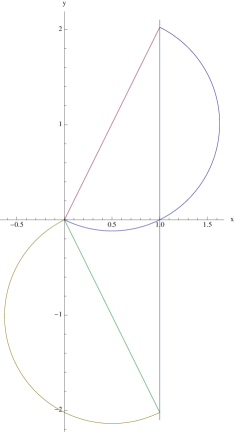
Figure 1: Case (III.1) is illustrated by drawing both ”half-circle” minimizers for arrival at $\left(x,\cdot,z\right)$ with $x=1,z=2$.

We analyze the Hamiltonian ODEs with boundary data (55). With $x_{0}=y_{0}=0$ and terminal conditions $x_{1}=x$ in (47) we have

$$rx = p_{0}\sin r-q_{0}\left(1-\cos r\right)$$

$$= p_{0}\sin r-2q_{0}\sin^{2}\frac{r}{2}.$$

Recall $q_{1}-q_{0}=\frac{r}{2}\left(x_{1}-x_{0}\right)$, a simple consequence from the Hamiltonian ODEs. Transversality condition $q_{1}=0$ (and $x_{1}=x,x_{0}=0$) then translates to $-2q_{0}=rx$. Plugging this into the previous equation leaves us with $rx\left(1+\cos r\right)=2p_{0}\sin r$. On the other hand, $z\neq 0\implies r\neq 0$ (no straight lines!) and we already pointed out in (51) that taking into account $z_{1}=z$ in (4.4.1), in addtion to $x_{0}=y_{0}=z_{0}=0$, gives

$$z=\frac{p_{0}^{2}+q_{0}^{2}}{2}\frac{r-\sin r}{r^{2}}.$$

Noting that $r-\sin r\neq 0$ when $r\neq 0$, it follows that

$$\frac{z\sin^{2}r}{r-\sin r} = \frac{4p_{0}^{2}\sin^{2}r+4q_{0}^{2}\sin^{2}r}{8r^{2}}$$

$$= x^{2}\frac{\left(1+\cos r\right)^{2}+\sin^{2}r}{8}=x^{2}\frac{1+\cos r}{4}.$$

If $\cos r=-1$ (equivalently: $r=\pi+2\pi\mathbb{Z}$) this equation is trivially satisfied; indeed both sides are zero since $\sin$ vanishes on $\pi+2\pi\mathbb{Z}$. Otherwise, the above equation may be written as

$$\frac{x^{2}}{z}=\frac{4\sin^{2}r}{\left(r-\sin r\right)\left(1+\cos r\right)}.$$ (56)

Focus on $z>0$ in the sequel, the other case being similar. Note that the right-hand-side above has a removable singularity at $r=\pi$ and takes, as $r\rightarrow\pi$, the value $8/\pi$. In fact, it is easy to see that the graph of the right-hand-side above as function of $r$ stays strictly below $8/\pi$ as $r\in\left(\pi,\infty\right)$. The assumption made in the (present) case III.1 is precisely $x^{2}/z<$ $8/\pi$. In particular then, each solution - there may be more than one - to (56), given $x^{2}/z\in[0,8/\pi)$, will be strictly bigger than $\pi$. We then have found the following possible values for $r:$

$$r\in\left\{\pm\pi,\pm 3\pi,...\right\}\cup\left\{\text{solutions to (\ref{LA_CaseIII_ratioxx_z}), "}>\pi\text{"}\right\}.$$

We can see that those values of $r$ for which $\left|r\right|$ is smallest correspond to the energy minimizing choice. Hence, in case (III.1), we have $r=\pm\pi$. Accordingly,

$$q_{0}=-\mathrm{sgn}\left(z\right)\pi x/2,\,\,\,p_{0}=\pm\sqrt{\frac{\pi}{4}\left(8\left|z\right|-\pi x^{2}\right)}$$

and also

$$p_{1}=0,\,y_{1}=\pm 2p_{0}/\pi,r=\pm\pi$$

which complements our apriori knowledge ($x_{1}=x,q_{1}=0,z_{1}=z$) of the Hamiltonian ODE solution at unit time. Note that we have two minimizing paths here, with respective arrival points $\left(x,\pm 2p_{0}/\pi,z\right)\in\left(x,\cdot,z\right)$. As usual, the energy is

$$\frac{1}{2}\left(p_{0}^{2}+q_{0}^{2}\right)=\left|z\right|\pi.$$

(The absence of $x$ in the energy is not surprising, since we are effectively dealing with (two) half-circles, radius (and then length) are fully determined by the prescribed area $z$.) Note that the energy function if smooth in a neighbourhood of $z$ since $z\neq 0$. At last, a computation gives

$$\frac{\partial\pi\mathrm{H}_{0\leftarrow 1}\left(x;y_{1},z,p_{1},q_{1},r\right)}{\partial\left(p_{1},y_{1},r\right)}=\left(\begin{array}[]{ccc}0&0&-\frac{y_{1}}{2}\\ \frac{2}{r}&0&\frac{x}{2}\\ \frac{rx+r\left(x+ry_{1}\right)}{2r^{2}}&-\frac{ry_{1}}{4}&0\end{array}\right),$$

the determinant of which equals

$$y_{1}^{2}/4=p_{0}^{2}/\pi^{2}=\frac{1}{4}\left(\frac{8}{\pi}\left|z\right|-x^{2}\right)>0$$

In particular, $\mathrm{x}_{0}=0$ is non-focal for $\left(x,\cdot,z\right)$ along either of the two minimizers. As a consequence, theorem 8 gives

$$f^{\varepsilon}\left(x,z;T\right)|_{T=1}\sim e^{-\left|z\right|\pi/\varepsilon^{2}}\varepsilon^{-2}c_{0}$$

in agreement with the corresponding expansion given in [45, Sec. 7, case (III.1)].

Case (III.2) Assume $\left|x\right|>\sqrt{8\left|z\right|/\pi}$ ($\implies x\neq 0$) and also $z\neq 0$; see figure 2.

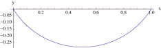
Figure 2: Case (III.2) is illustrated by drawing the unique minimizing arc for arrival at $\left(x,\cdot,z\right)$ with $x=1,z=1/5$.

(The case $z=0$ is simpler and discussed separately below). We proceed exactly as above, but now there is a (unique) solution $r_{0}:=r\in(-\pi,\pi)\backslash\left\{0\right\}$ to (56), which corresponds to the energy correspond to the energy minimizing choice. We then find

$$p_{1}=x\frac{r}{2}\cot\frac{r}{2},\,y_{1}=0,r=r_{0}$$

which complements our apriori knowledge ($x_{1}=x,q_{1}=0,z_{1}=z$) of the Hamiltonian ODE solution at unit time. (The results corresponds precisely to the point-point problem discussed in case (I.2) with arrival point $\left(x,0,z\right)$.) A computation then shows that

$$\frac{\partial\pi\mathrm{H}_{0\leftarrow 1}\left(x;y_{1},z,p_{1},q_{1},r\right)}{\partial\left(p_{1},y_{1},r\right)}|=\left(\begin{array}[]{ccc}-\frac{\sin r}{r}&\frac{\sin r}{r}&\frac{x\cot\left(\frac{r}{2}\right)\left(-r+\sin r\right)}{2r}\\ \frac{1-\cos r}{r}&\cos^{2}\frac{r}{2}&\frac{x\left(r-\sin r\right)}{2r}\\ \frac{x}{r}-\frac{1}{2}x\cot\frac{r}{2}&\frac{1}{4}rx\cot\frac{r}{2}&\frac{x^{2}\left(-2+r\cot\frac{r}{2}\right)\cot\frac{r}{2}}{4r}\end{array}\right),$$

the determinant of which simplifies to

$$\frac{x^{2}\left(-2+r\cot\frac{r}{2}\right)\cot\frac{r}{2}}{r}\text{. }$$

Since $x\neq 0$, it suffices to remark that the remaining factor, as function of $r$ only, does not take the value zero for $r\in\left(-\pi,\pi\right)\backslash\left\{0\right\}$. In fact, as is easy to see, the determinant has a removable singularity at zero remains strictly negative on the entire open interval $\left(-\pi,\pi\right)$. We thus established non-focality (note however, that the determinante does vanish in the limit $\left|r\right|\uparrow\pi$; this is the focal case (III.4) discussed below.) Theorem 8 then gives

$$f^{\varepsilon}\left(x,z;T\right)|_{T=1}\sim e^{-c_{1}/\varepsilon^{2}}\varepsilon^{-2}c_{0}$$

where $c_{1}$ is determined exactly as in case (I.2), equation (54), just with $y=y_{1}=0$.

Case (III.3) Assume $\left|x\right|>\sqrt{8\left|z\right|/\pi}=0$ (i.e. $x\neq 0,\,z=0$) One finds without trouble $r=0,\,p_{0}=x,q_{0}=0$ and then $p_{1}=x,y_{1}=0$; from transversality of course $q_{1}=0$. The (unique) minimizing path is then given by $\left(x_{t},y_{t}\right)=\left(tx,0\right)$, the energy is equal to $\left|x\right|$. Non-focality can be checked e.g. by recycling the expression of case (III.2) in the limit $r=0$.

Case (III.4) All computations from either case (III.1) remain valid. We have $y_{1}=0$ (so that there is a unique minimizer) and the determinant, which was seen to be $\propto y_{1}^{2}$ is now equal to zero. By definition, $\mathrm{x}_{0}=0$ is then focal for $\left(x,\cdot,z\right)$ along the (now: unique) minimizer. Equivalently, we may approach this from case (III.2), by taking the limit $\left|r\right|\uparrow\pi$ (geometrically this amounts to have more and more curved arcs from $\left(0,0\right)$ to $\left(x,0\right)$ until we arrive at the half-circle solution from). Either way, being in a focal situation, we cannot apply theorem 8 and indeed in [45] a density expansion is given with algebraic factor $\varepsilon^{-5/2}$, in contrast to the generic prediction $\varepsilon^{-l},\,l=2$ of our theorem.

4.4.2 Starting point with O($\varepsilon)$-dependence; appearance of $e^{c_{2}/{\varepsilon}}$-factor

Let us briefly illustrate how our methods allow to go beyond the results of Takanobu–Watanabe, which are - in the non-degenerate case - marginal density expansions based on (45), started at the origin and run til unit time ($T=1$), of the form

$$\bar{f}^{\varepsilon}\left(\mathrm{a}\right)|\sim e^{-c_{1}/\varepsilon^{2}}\varepsilon^{-l}c_{0}\text{ with }c_{1}=\Lambda\left(\mathrm{a}\right)\text{ and }c_{0}>0.$$

For instance, in the case (III) above, we have $\mathrm{a}=\left(x,z\right)\in\mathbb{R}^{l}$ for $l=2$. To this end, we again consider marginal density expansions based on (45), but now started order $\varepsilon$ away from the origin. For simplicity only, we shall consider the subcase (III.1), the energy in this case was computed to be $\Lambda\left(\mathrm{a}\right)=\Lambda\left(x,z\right)=\pi|z|$, and take the starting point

$$X_{0}=0,\,Y_{0}=\varepsilon\hat{y}_{0},\,Z_{0}=\varepsilon\hat{z}_{0}.$$

According to our general theory, as laid out in theorem 8, perturbation of the starting point to first order in $\varepsilon$ will lead to appearance of second order exponential terms in the density (at time $T=1$),

$$f^{\varepsilon}\left(\mathrm{a}\right)\sim e^{-c_{1}/\varepsilon^{2}}e^{c_{2}/\varepsilon}\varepsilon^{-l}c_{0}.$$

We now compute $c_{2}$. With ^′ for the derivative with respect to $\mathrm{a}=\left(x,z\right)$ as usual, we have, assuming $z>0$ w.l.o.g.,

$$\Lambda^{\prime}\left(\mathrm{a}\right)=\left(\partial_{x}\Lambda\left(x,z\right),\partial_{z}\Lambda\left(x,z\right)\right)=\left(0,\pi\right).$$

On the other hand, we need to compute $\mathrm{\hat{Y}}_{T}=\left(\hat{X}_{T},\hat{Z}_{T}\right)$, along (apriori each of the two) minimizing controls $\mathrm{h}=\left(h^{1},h^{2}\right)$, based on the following auxilary ODE,

$$d\hat{X} = 0,d\hat{Y}=0,d\hat{Z}=-\frac{1}{2}\hat{Y}dh^{1}+\frac{1}{2}\hat{X}dh^{2},$$

$$\hat{X}_{0} = 0,\,\hat{Y}_{0}=\hat{y}_{0},\,\hat{Z}_{0}=\hat{z}_{0}.$$

Noting that $\mathrm{h}_{0}=\left(0,0\right),\,\mathrm{h}_{T}\in\left(x,\cdot\right)$, and thanks to $\hat{X}\equiv 0$, the computation is identical for both controls, $\hat{Z}_{T}=\hat{z}_{0}-\hat{y}_{0}x/2$. And it follows that $c_{2}=\Lambda^{\prime}\left(\mathrm{a}\right)\cdot\mathrm{\hat{Y}}_{T}=\pi\left(\hat{z}_{0}-\hat{y}_{0}x/2\right)$. We thus proved

Proposition 23

Let $\left(X^{\varepsilon},Y^{\varepsilon},Z^{\varepsilon}\right)$ be $\varepsilon$-dilated Brownian motion on the Heisenberg group, started at $\left(0,\varepsilon\hat{y}_{0,}\varepsilon\hat{z}_{0}\right)$. Then $\left(X_{1}^{\varepsilon},Z_{1}^{\varepsilon}\right)$ admits a density which in the case (III.1), say when $z>0$ and $\left|x\right|<$ $\sqrt{8z\pi}$, has an expansion as $\varepsilon\to 0$, for some $c_{0}>0$, of the form

$$f_{\varepsilon}\left(x,z;T\right)|_{T=1}\sim e^{-\pi z/\varepsilon^{2}}e^{\pi\left(\hat{z}_{0}-\hat{y}_{0}x/2\right)/\varepsilon}\varepsilon^{-2}c_{0}.$$ (57)

Note that, upon taking $\hat{y}_{0}=\hat{z}_{0}=0$, we recover the previous expansion of case (III.1),

$$\bar{f}^{\varepsilon}\left(x,z\right)\sim e^{-\pi z/\varepsilon^{2}}\varepsilon^{-2}c_{0}.$$

Other cases than (III.1), and also $\hat{X}_{0}=\hat{x}_{0}\neq 0$, are treated similarly but the computations are more involved. Let us, instead, verify (57) by a reduction to the zero starting point case, using the Heisenberg group structure. Namely,

$$\left(\bar{X}^{\varepsilon},\bar{Y}^{\varepsilon},\bar{Z}^{\varepsilon}\right):=\left(0,-\varepsilon\hat{y}_{0},-\varepsilon\hat{z}_{0}\right)\ast\left(X^{\varepsilon},Y^{\varepsilon},Z^{\varepsilon}\right)$$

satisfies the same stochastic differential equations, but now started at the origin. In particular,

$$\left(\bar{X}_{T}^{\varepsilon},\bar{Z}_{T}^{\varepsilon}\right)=\left(X_{T}^{\varepsilon},Z_{T}^{\varepsilon}-\varepsilon\left(\hat{z}_{0}+\hat{y}_{0}X_{T}^{\varepsilon}/2\right)\right)$$

and so

$$f^{\varepsilon}\left(x,z\right) = \bar{f}^{\varepsilon}\left(x,z-\varepsilon\left(\hat{z}_{0}+\hat{y}_{0}x/2\right)\right)$$

$$\sim e^{-\pi\left(z-\varepsilon\left(\hat{z}_{0}+\hat{y}_{0}x/2\right)\right)/\varepsilon^{2}}\varepsilon^{-2}c_{0}$$

$$\sim e^{-\pi z}e^{\pi\left(\hat{z}_{0}-\hat{y}_{0}x/2\right)/\varepsilon}\varepsilon^{-2}c_{0}.$$

in agreement with the above proposition (the constant $c_{0}$ was allowed to change here). It is not hard to devise variations on the theme (in particular, upon inclusion of drift vector fields of order $\varepsilon$) where theorem 8 still applies but the above reasoning based on the (rigid) Heisenberg group structure fails.

References

• [1] R. Azencott. Formule de Taylor stochastique et développement asymptotique d’intégrales de Feynmann. Séminaire de Probabilités XVI; Supplément: Géométrie différentielle stochastique. Lecture notes in Mathematics, 921, 237-285, 1982.
• [2] R. Azencott. Petites perturbations aléatoires des systèmes dynamiques: développements asymptotiques. Bulletin des sciences mathématiques. vol. 109, no3, pp. 253-308, 1985.
• [3] G. Ben Arous. Développement asymptotique du noyau de la chaleur hypoelliptique hors du cut-locus. Annales Scientifiques de l’Ecole Normale Supérieure, 4 (21): 307-331, 1988.
• [4] G. Ben Arous. Methods de Laplace et de la phase stationnaire sur l’espace de Wiener. Stochastics, 25: 125-153, 1988.
• [5] G. Ben Arous, R. Léandre: Décroissance exponentielle du noyau de la chaleur sur la diagonale (I), Probab. Th. Rel. Fields 90, 175-202 (1991)
• [6] G. Ben Arous and R. Léandre, Décroissance exponentielle du noyau de la chaleur sur la diagonale (II), Probab. Theory Related Fields, 90, 377-402 (1991)
• [7] G. Ben Arous, R. Léandre: Décroissance exponentielle du noyau de la chaleur sur la diagonale (II), Probab. Th. Re1. Fields 90, 377-402,1991.
• [8] G. Ben Arous, P. Laurence: Second order expansion for implied volatility in two factor local-stochastic volatility models and applications to the dynamic Sabr model. Preprint 2010.
• [9] R. Bishop, R. Crittenden, Geometry of Manifolds, Academic Press 1964.
• [10] H. Berestycki, J. Busca, and I. Florent. Computing the implied volatility in stochastic volatility models. Communications on Pure and Applied Mathematics, 57(10):1352-1373, 2004.
• [11] J.M. Bismut. Malliavin Calculus and Large Deviations. volume 45 of Progress in Mathematics. Birkhäuser Boston Inc., Boston, MA, 1984.
• [12] P Bourgade and O Croissant. Heat kernel expansion for a family of stochastic volatility models : delta-geometry; arXiv:cs.CE/0511024, 2005.
• [13] do Carmo, M. , “Riemannian Geometry”, Birkhaeuser (1992).
• [14] J.D. Deuschel, P.K. Friz, A. Jacquier, S. Violante. Marginal density expansions for diffusions and stochastic volatility, part II: Applications. Communications on Pure and Applied Mathematics, to appear.
• [15] J.D. Deuschel and D.W. Stroock. Large Deviations. Volume 342 of AMS/Chelsea Series. 2000.
• [16] M. Freidlin and A.D. Wentzell. Random perturbations of dynamical systems. Grundlehren der Mathematischen Wissenschaften (Second edition ed.). New York: Springer-Verlag, 1998.
• [17] P. Friz, S. Gerhold, A. Gulisashvili and S. Sturm. Refined implied volatility expansions in the Heston model. Quant. Finance, Volume 11, Issue 8, 1151-1164, 2011.
• [18] Friz, Peter; Oberhauser, Harald A generalized Fernique theorem and applications, Proceedings of the American Mathematical Society, 138 (2010), 3679-3688. ISSN 0002-9939. Publisher: AMS, US
• [19] Friz, Peter; Victoir, Nicolas; Multidimensional Stochastic Processes as Rough Paths. Theory and Applications, Cambridge Studies of Advanced Mathematics Vol. 120, 670 p., Cambridge University Press
• [20] Gaveau B.: Principe de moindre action, propagation de la chaleur et estimées sous-elliptiques sur certains groupes nilpotents. Acta. Math. 139 (1977), 95- 153.
• [21] Gatheral, Jim; Hsu, Elton P.; Laurence, Peter; Ouyang, Cheng; Wang, Tai-Ho. Asymptotics of Implied Vol in Local Vol Models. Math. Finance, Volume 22, Issue 4, pages 591–620, October 2012
• [22] R. Giambo, F. Giannoni, P. Piccione and D. V. Tausk, Morse theory for normal geodesics in sub-Riemannian manifolds with codimension one distributions, Topological Methods in Nonlinear Analysis, Journal of the Julius Schauder Center Volume 21, 2003, 273–291
• [23] A. Gulisashvili and E. Stein. Asymptotic Behavior of the Stock Price Distribution Density and Implied Volatility in Stochastic Volatility Models, Applied Mathematics & Optimization, Volume 61, Number 3, 287-315, DOI: 10.1007/s00245-009-9085-x
• [24] I. Gyöngy. Mimicking the one-dimensional marginal distributions of processes having an Itô differential. Probab. Theory Relat. Fields, 71(4):501–516, 1986
• [25] N. Ikeda and S. Watanabe, Stochastic differential equations and diffusion processes, North-Holland Mathematical Library, vol. 24, North-Holland, Publishing Co., Amsterdam, 1981.
• [26] Patrick Hagan, Andrew Lesniewski, and Diana Woodward; Probability Distribution in the SABR Model of Stochastic Volatility. Working Paper 2005. Available on lesniewski.us/working.html
• [27] Henry-Labordère P, Analysis, geometry and modeling in finance, Chapman and Hill/CRC, 2008.
• [28] Jurdjevic, Kupka; Polynomial Control Systems; Math. Ann. 272, 361-368 (1985)
• [29] V. Jurdjevic; Geometric Control Theory; CUP (1996)
• [30] Yu. I. Kifer, “On the asymptotics of the transition probability density of processes with small diffusion”, Teor. Veroyatnost. i Primenen., 21:3 (1976), 527–536
• [31] H. Kunita, Supports of diffusion processes and controllability problems. Proc. Intern. Symp. SDE Kyoto 1976, 163-185, Kinokuniya, Tokyo, 1978.
• [32] S. Kusuoka and Y. Osajima: A remark on the asymptotic expansion of density function of Wiener functionals. Journal of Functional Analysis, Volume 255, Issue 9, 1 November 2008, Pages 2545–2562, Special issue dedicated to Paul Malliavin
• [33] S. Kusuoka and D. W. Stroock, Precise asymptotics of certain Wiener functionals. Journal of Functional Analysis, Volume 99, Issue 1, July 1991, Pages 1-74.
• [34] L. Mesnager, Etude en temps petit de densités conditionnelles dans des problèmes de Filtrage Non Linéaire. Travaux Universitaires - Thèse nouveau doctorat, 126 pages. Université de Paris 11, Orsay. 1996.
• [35] S. A. Molchanov, Diffusion processes and Riemannian geometry, Russ. Math. Surv., 1975, 30 (1), 1–63.
• [36] R. Montgomery. A Tour of SubRiemannian Geometries, their Geodesics and Applications, Volume 91 of Mathematical Surveys and Monographs. American Mathematical Society, Providence, RI, 2002.
• [37] D. Nualart. The Malliavin Calculus and Related Topics. Springer-Verlag, Berlin, second edition, 2006.
• [38] Osajima, Yasufumi, General Asymptotics of Wiener Functionals and Application to Mathematical Finance (July 25, 2007). Available at SSRN: http://ssrn.com/abstract=1019587
• [39] Paulot, Louis, Asymptotic Implied Volatility at the Second Order with Application to the SABR Model (June 3, 2009). Available at SSRN: http://ssrn.com/abstract=1413649
• [40] Huyên Pham, Large deviations in Finance, 2010, Third SMAI European Summer School in Financial Mathematics.
• [41] V. Piterbarg, Markovian projection method for volatility calibration; Risk, April 2007, available at SSRN: http://ssrn.com/abstract=906473, 2006.
• [42] Sakai, T.: Riemannian Geometry, AMS, 1992.
• [43] Seierstad, A. and Sydsaeter, K.: Optimal Control Theory with Economic Applications. (Advanced Textbooks in Economics, 24). North- Holland Amsterdam, 1987
• [44] Stein, E. M., and J. C. Stein, 1991, “Stock Price Distributions with Stochastic Volatility: An Analytic Approach,” Review of Financial Studies, 4, 727-752.
• [45] Takanobu S. Watanabe S.: Asymptotic expansion formulas of the Schilder type for a class of conditional Wiener functional integration. In “Asymptotics problems in probability theory: Wiener functionals and asymptotics”. K.D. Elworthy N. Ikeda edit. Pitman. Res. Notes. Math. Series. 284 (1993), 194-241.
• [46] Varadhan, S. R. S., On the behavior of the fundamental solution of the heat equation with variable coefficients. Communications on Pure and Applied Mathematics, 20: 431–455. 1967
• [47] Varadhan, S.R.S.: Lectures on large deviations, available at http://math.nyu.edu/faculty/varadhan/LDP.html, 2010.