POISSON project – II – A multi-wavelength spectroscopic and photometric survey of young protostars in L 1641

Abstract

Context. Characterising stellar and circumstellar properties of embedded young stellar objects (YSOs) is mandatory for understanding the early stages of the stellar evolution. This task requires the combination of both spectroscopy and photometry, covering the widest possible wavelength range, to disentangle the various protostellar components and activities.

Aims. As part of the POISSON project (Protostellar Optical-Infrared Spectral Survey On NTT), we present a multi-wavelength spectroscopic and photometric investigation of embedded YSOs in L 1641, aimed to derive the stellar parameters and evolutionary stages and to infer their accretion properties.

Methods. Our multi-wavelength database includes low-resolution optical-IR spectra from the NTT and Spitzer (0.6-40 $\mu$m) and photometric data covering a spectral range from 0.4 to 1100 $\mu$m, which allow us to construct the YSOs spectral energy distributions (SEDs) and to infer the main stellar parameters (visual extinction, spectral type, accretion, stellar, bolometric luminosity, mass accretion and ejection rates).

Results. The NTT optical-NIR spectra are rich in emission lines, which are mostly associated with YSO accretion, ejection, and chromospheric activities. A few emission lines, prominent ice (H₂O and CO₂), and amorphous silicate absorption features have also been detected in the Spitzer spectra. The SED analysis allows us to group our 27 YSOs into nine Class I, eleven Flat, and seven Class II objects. However, on the basis of the derived stellar properties, only six Class I YSOs have an age of $\sim$10⁵ yr, while the others are older (5$\times$10⁵–10⁶ yr), and, among the Flat sources, three out of eleven are more evolved objects (5$\times$10⁶–10⁷ yr), indicating that geometrical effects can significantly modify the SED shapes. Inferred mass accretion rates ($\dot{M}_{acc}$) show a wide range of values (3.6$\times$10^-9 to 1.2$\times$10^-5 M_☉ yr^-1), which reflects the age spread observed in our sample well. Average values of mass accretion rates, extinction, and spectral indices decrease with the YSO class. The youngest YSOs have the highest $\dot{M}_{acc}$, whereas the oldest YSOs do not show any detectable jet activity in either images and spectra. Apart from the outbursting source # 25 and, marginally, # 20, none of the remaining YSOs is accretion-dominated ($L_{acc}>L_{*}$). We also observe a clear correlation among the YSO $\dot{M}_{acc}$, $M_{*}$, and age. For YSOs with $t>10^{5}$ yr and $0.4\,M_{\sun}\leq M_{*}\leq 1.2$ $M_{\sun}$, a relationship between $\dot{M}_{acc}$ and $t$ ($\dot{M}_{acc}\propto t^{-1.2}$) has been inferred, consistent with mass accretion evolution in viscous disc models and indicating that the mass accretion decay is slower than previously assumed. Finally, our results suggest that episodic outbursts are required for Class I YSOs to reach typical classical T Tauri stars stellar masses.

1 Introduction

Our working model of low-mass star formation arises from a combination of the empirical classification of the YSO SEDs (Lada & Wilking, 1984; Lada, 1987) with a theoretical picture of YSO formation, which involves the collapse of an isolated rotating dense core, which then forms an accreting protostellar core and a disc (Adams & Shu, 1986; Adams et al., 1987). The empirical evolutionary sequence goes from Class 0 to III objects. Class 0 YSOs are the youngest sources ($\sim$10⁴ yr), while Class III (the so-called weak T Tauri stars) are the oldest ones (10⁷ yr). The classification of Class I, II, and III objects is based on the slope of the SED between 2 and 20 $\mu$m ($\alpha_{2-20\,\mu m}$), defined as $\alpha=dLog(\lambda F_{\lambda})/dLog(\lambda)$ (Lada, 1987). On the other hand, Class 0 YSOs, which are usually not visible at these wavelengths, are defined as having $L_{smm}/L_{bol}>$0.5%, where $L_{smm}$ is measured longward of 350 $\mu$m (Andre et al., 1993, 2000), and they have more than 50% of their mass in the surrounding envelope. The youngest protostars (0, I) are thus extremely embedded, and are characterised by steeply rising SEDs from near to far-IR, mostly or entirely coming from the emission of their surrounding envelope. According to this picture, most (in the case of Class I YSOs) or all (in the case of Class 0 YSOs) the YSO luminosity is believed to come from accretion ($L_{bol}\sim L_{acc}\sim GM{{}_{*}}\dot{M}_{acc}/R_{*}$) through a circumstellar disc. Part of the accreted material ($\sim$10%) is ejected by means of powerful collimated jets. The more evolved Class II and III sources instead have smaller IR excesses, and their SEDs can be modelled well by pre-main sequence photospheres surrounded by circumstellar discs (i. e., classical T Tauri stars - CTTs). The luminosity of these ‘older’ objects mostly originates in their stellar photosphere, rather than from accretion processes. Thus, accretion and ejection activities are strongly reduced or even absent in the latest stages.

Our understanding of the YSO early evolutionary stages (Class 0 and I), mostly relies on SED analysis or, indirectly, on studies of their jets and outflows. On the other hand, we have a clearer picture of the latest stages, for which the physical properties of the accreting protostars can be well studied and characterised. Recent theoretical studies on SEDs (Whitney et al., 2003a, b; Robitaille et al., 2007) have shown that the SED analysis alone may not be sufficient to disentangle the YSO evolutionary stage, and NIR spectroscopy is needed to characterise the embedded accreting protostellar core. For example, geometrical effects may produce SED misclassifications, i. e. old objects observed edge-on may show Class I shapes, or young YSOs face-on may appear older, showing Class II SED shapes. Thus, a correct classification can be only obtained from the combined analysis of the YSO SED and the characterisation of the embedded stellar object and its activity. Quantitative information on the various phenomena characterising the environment of young stars can be derived from NIR spectroscopic studies, which allow us to observe embedded objects, and investigate processes occurring in regions spatially unresolved, like the accretion funnel flows, and the ejection of jets from the adjacent inner disc, by using features related to the different emitting regions.

These considerations have recently triggered a series of observational studies, aimed at deriving the stellar physical properties and evolutionary status of the embedded YSOs, in particular of the Class I YSOs, which are visible at IR wavelengths. As a result, these studies have indicated that only a fraction of Class I sources is composed of highly accreting objects (see, e. g. White & Hillenbrand, 2004; Nisini et al., 2005a; Doppmann et al., 2005; Antoniucci et al., 2008), which show evidence of jet activity. Several objects, classified as Class I, have indeed mass accretion/ejection rates similar to those of Class II. Some of them are mis-classified, whereas others appear to be bona-fide young embedded objects (White et al., 2007). Indeed, the so far studied sample is still limited, biased, and mostly confined to a few selected star-forming regions (i. e. mostly Taurus, see, e. g., White et al., 2007; Beck, 2007; Prato et al., 2009).

In this framework, we have undertaken a combined optical/IR unbiased spectroscopic survey on a flux-limited sample of selected Class I/II sources, located in six different nearby clouds (namely Cha I & II, L 1641, Serpens, Lupus, Vela, and Corona Australis; see, Antoniucci et al., 2011, hereafter paper-1), using the EFOSC2/SOFI instruments on the ESO-NTT (POISSON: Protostellar Objects IR-optical Spectral Survey On NTT). In paper-1 we presented the results of the Cha I & II regions, comparing $L_{acc}$ determinations from the different tracers, and discussing the reliability and consistency of the different empirical relationships considered. In this paper we report the survey results on L 1641, largely complemented by archive and literature data, which allow us to characterise the studied YSOs.

At a distance of 450 pc, the Lynds 1641 molecular cloud (L 1641) is part of the Orion GMC complex (for a complete review see, Allen & Davis, 2008). Southward of the ONC, L 1641 extends from NW to SE for $\sim$2.5$\degr$, and contains hundreds of young stellar objects, ranging from high- to low-mass YSOs. Moreover, the L 1641 cloud has been producing stars for nearly 30 Myr (Allen, 1995), thus it harbours a very heterogeneous sample of YSOs, which span from extremely active and young to old and quiet objects, making it the perfect candidate to study the different YSO evolutionary stages in an unbiased fashion. Our observations were performed on 27 embedded YSOs selected in L 1641 on the basis of the brightness and SED spectral index ($\alpha$). Our multi-wavelength database includes low-resolution optical-IR spectra from the NTT and Spitzer (0.6-40 $\mu$m), as well as photometric data covering the spectral range from 0.4 to 1100 $\mu$m, which allow us to construct the YSO SEDs and to characterise the object parameters (visual extinctions, spectral types, accretion and bolometric luminosities, mass accretion and ejection rates).

This paper is organised as follows. Section 2 describes the selection criteria for our YSO sample. In Section 3 we define our observations, data reduction, and the collected literature data. In Section 4 we report on the results obtained from our photometry and spectroscopy, we describe the detected spectral features and characterise the YSOs. In Section 5 we discuss the accretion properties of the sample, as well as the origin of the observed mass accretion evolution. Finally, our conclusions are drawn in Section 6.

2 Sample definition

Our sample of YSOs in L 1641 was selected from Chen & Tokunaga (1994) on the basis of the SED spectral index ($\alpha$) and NIR brightness of each source, because of the instrumental sensitivity. In particular, we chose those objects showing $\alpha>$-0.4 and $K^{\prime}\leq$12 mag, implying that most of our targets are, in principle, Class I and flat YSO candidates. According to te latest Spitzer surveys, this brightness constraint limits our study to about 15% of the entire embedded population in L 1641 (see, Allen & Davis, 2008, and references therein).

It is worth noting that the $\alpha$ classification in Chen & Tokunaga (1994) is based on $K^{\prime}$ and $IRAS$ 25 $\mu$m photometry, and, as it will be shown in Sect. 3.3 and Sect. 4.4.2, often differs from the 2MASS/Spitzer classification obtained in this paper (Sect. 4.4.2). This is mostly due to the low spatial resolution of the IRAS beam (1$\arcmin\times$5$\arcmin$ at 25 $\mu$m) that is not enough to properly resolve different sources in crowded regions such as L 1641. As a result, the 27 YSOs are grouped into nine Class I, eleven Flat, and seven Class II objects. Additionally, some targets identified as single sources in Chen & Tokunaga (1994) turned out to be double YSOs after analysing the Spitzer images (namely [CTF93]146, [CTF93]216, [CTF93]237, and [CTF93]245B).

The targets, along with their ID, $SIMBAD$ name, and coordinates (J2000.0), are listed in Table 1 (Columns 1–5). The sources have been named following the nomenclature of Chen et al. (1993) with the exception of those identified here as double YSOs, which have been labelled as “ target-1” , when coincident or closest to the literature coordinates, and “ target-2” , the farthest. The large separations ($\geq$40$\arcsec$) exclude that these sources are physically bound, with the exception of sources [CTF93]237, separated less than 5$\arcsec$ ($\sim$2250 AU at 450 pc). Another exception might be [CTF93]216-1 and [CTF93]216-2. They might be part of a wide binary system (35$\arcsec\sim$15 700 AU, at d=450 pc), and both sources show two precessing jets in the Spitzer images (see also Fig. 16 in Appendix B). However such a wide system would not produce precessing jets, thus it is more likely that both sources are binary systems.

Table 1: Targets and Observations.

ID	Target name	Other Name	$\alpha$ (J2000.0)			$\delta$ (J2000.0)			Spectroscopy
			(h	m	s)	($\degr$	$\arcmin$	$\arcsec$)
1	[CHS2001]13811	2MASS-J05360665-0632171	05	36	06.65	-06	32	17.1	O,B,R,S
2	[CTF93]50	NAME HH 147MMS	05	36	25.13	-06	44	41.8	O,B,R,S
3	[CTF93]47	V* V380 Ori	05	36	25.43	-06	42	57.7	O,B,R
4	[CTF93]32	V* V846 Ori	05	36	41.34	-06	34	00.3	O,B,R,S
5	[CTF93]72	IRAS 05350-0700	05	37	24.47	-06	58	32.9	O,B,R,S
6	[CTF93]83	HH 43 IRS1	05	38	07.44	-07	08	30.0	R,S
7	[CTF93]62	V* V1787 Ori	05	38	09.23	-06	49	15.9	O,B,R,S
8	[CTF93]79	V* V883 Ori	05	38	18.10	-07	02	25.9	O,B,R
9	[CTF93]99	Haro 4-254	05	38	52.36	-07	21	09.5	O,B,R,S
10	[CTF93]87	2MASS-J05390536-0711052	05	39	05.36	-07	11	05.2	O,B,R,S
11	[CTF93]104	HBC 176	05	39	22.32	-07	26	44.5	O,B,R
12	Meag31	2MASS-J05401379-0732159	05	40	13.79	-07	32	15.9	B,R
13	[CTF93]146-2	2MASS-J05401494-0748485	05	40	14.94	-07	48	48.5	R,S
14	[CTF93]146-1	IRAS 05378-0750	05	40	17.80	-07	48	25.8	R,S
15	[CTF93]211	IRAS 05379-0815	05	40	19.40	-08	14	16.3	O,B,R,S
16	[CTF93]187	V* V1791 Ori	05	40	37.36	-08	04	03.0	O,B,R,S
17	[CTF93]168	IRAS 05389-0759	05	41	22.13	-07	58	03.0	R,S
18	[CTF93]191	V* DL Ori	05	41	25.34	-08	05	54.7	O,B,R,S
19	[CTF93]246A	2MASS-J05413005-0840092	05	41	30.05	-08	40	09.2	R,S
20	[CTF93]186	IRAS 05391-0805	05	41	30.22	-08	03	41.4	R,S
21	[CTF93]246B	2MASS-J05413033-0840177	05	41	30.33	-08	40	17.7	R,S
22	[CTF93]237-2	2MASS-J05413418-0835273	05	41	34.18	-08	35	27.3	R,S
23	[CTF93]237-1	IRAS 05391-0836	05	41	34.78	-08	35	23.0	R,S
24	[CTF93]216-1	IRAS 05403-0818	05	42	47.06	-08	17	06.9	R,S
25	[CTF93]216-2	2MASS-J05424706-0817069	05	42	48.48	-08	16	34.7	R,S
26	[CTF93]245B-2	[BDB2003]G212.98-19.15	05	42	50.48	-08	38	29.2	O,B,R
27	[CTF93]245B-1	IRAS 05404-0841	05	42	50.50	-08	39	57.6	B,R

3 Observations and data reduction

Our multi-wavelength database on L 1641 targets is made of: i) low-resolution optical and NIR spectroscopic observations from the ESO/NTT, to infer most of the YSO main stellar parameters (spectral type, accretion, mass accretion and ejection rates); ii) archival Spitzer-IRS spectra, mostly used to derive the visual extinction; iii) Spitzer-IRAC and Spitzer-MIPS images from the Spitzer Heritage Archive, and literature photometric data, covering a spectral range from 0.4 to 1100 $\mu$m, which allow us to construct the SEDs.

3.1 Optical and NIR spectroscopy

Our optical and near-infrared spectroscopic observations were obtained at the ESO New Technology Telescope with EFOSC2 (Buzzoni et al., 1984) and SofI (Moorwood et al., 1998), respectively. The observations were carried out over a short period of time (10-13 and 14-16 February 2009, for the NIR and optical spectroscopy, respectively), thus possible YSO variability should not significantly affect the optical and NIR segments of our spectra. The observational settings (spectral resolution and slit width) were chosen to obtain, as far as possible, homogeneous spectra, aiming to apply a combined optical/NIR analysis. The total integration time on source (I_t) in both optical and NIR spectra differs from target to target, depending on the source brightness, which was chosen to obtain a signal to noise ratio $\geq$200 on the continuum and detect emission lines, which are 1/20 of the continuum, with at least S/N = 10. No preferential position angles for the slits were chosen.

The EFOSC2 spectra were taken with the grism N.16 and a 0$\aas@@fstack{\prime\prime}$7 slit width, covering a wavelength range from $\sim$0.6 to 1 $\mu$m, and with a spectral resolution of R$\sim$700. I_t ranges from 30 s (targets with $V$=11 mag) up to 1800 s (targets with $V$=17 mag). Only those targets having a $V$ band magnitude $\leq$17 were observed (namely 14 out of 27 objects), and they are indicated in our observation log of Table 1 (column 6) with the label ‘O’.

The SofI NIR spectra were taken with an AB offset scheme. We used a 0$\aas@@fstack{\prime\prime}$6 slit (R$\sim$900) for both the blue grism (ranging from 0.95 to 1.64 $\mu$m, and labelled as ‘B’ in column 6 of Tab. 1) and the red grism (ranging from 1.51-2.5 $\mu$m, and labelled as ‘R’ in column 6 of Tab. 1). Only those targets with J$\leq$15 mag were observed with the blue grism (namely 16 out of 27 targets), whereas all the targets were observed with the red grism. I_t ranges from 20 s (objects with J=8 mag) up to 1200 s (objects J$\geq$13 mag) in the blue grism, and from 20 s (targets with K=5 mag) up to 1800 s (K$\geq$12 mag) in the red grism.

Additionally, telluric and spectro-photometric standards were observed to correct for the atmospheric spectral response and to flux-calibrate the spectra, respectively. In particular HD 289002 (B3 spectral type) was chosen for the optical spectra, whereas an F8V type star (Hip 23930) was selected for the NIR.

The data reduction was done using standard IRAF tasks. Each spectrum segment was flat fielded, sky subtracted and corrected for the curvature derived from long-slit spectroscopy, while atmospheric features were removed by dividing the spectra by the telluric standard star. The wavelength calibrations were performed using a helium-argon lamp in the optical and a xenon lamp in the infrared. The resulting spectra were originally flux calibrated by means of the observed standard stars. We thus obtained for each target up to three individually calibrated spectra (optical, blue and red grism). However, due to variable seeing conditions during our observations (from 0$\aas@@fstack{\prime\prime}$6 to 1$\aas@@fstack{\prime\prime}$3) and SofI instrumental problems (the source did not remain correctly centred on the slit during the nodding cycle), often the stellar calibrated continua do not properly match in the three spectral segments. Thus, we performed aperture photometry on the $K_{s}$ band SofI acquisition images (see Sect. 3.3), to get an absolute flux-calibration for the red grism spectra, and match to these the stellar continua of the two remaining segments, finally obtaining a single flux-calibrated spectrum from 0.6 to 2.5 $\mu$m. Uncertainties on the $K_{s}$ photometry range from $\sim$5 to 10% of the total flux.

3.2 Archival Spitzer spectroscopy

From the Spitzer Heritage Archive we retrieved 20 spectra (the spectrum of [CTF93]50 - #2 - has already been presented by Fischer et al., 2010), which were labelled as ‘S’ in column 6 of Tab. 1. [CTF93]237-1 and -2 are not spectrally resolved, thus the spectra are blended. No additional data are available in the archive for the remaining objects in the Spitzer archive.

All the data were taken with the Spitzer Infrared Spectrograph (IRS; Houck et al., 2004) under a variety of programs (namely 30706, 30859, and 50374), and observed between November 2006 and November 2008. All the IRS spectra were obtained with a combination of short-low (SL2/SL1, 5.2-8.7/7.4-14.5 $\mu$m, R = 64-128), and long-low (LL, 14.0-39.0 $\mu$m, R = 64-128) modules (i. e. ranging from 5 to 39 $\mu$m). Source # 9 was observed with the LL module alone. The total exposure time on source ranges from four to eight minutes. All the spectra were observed in IRS staring mode and extracted from the Spitzer Science Center S18.7.0 pipeline basic calibrated data (BCD) using the Spitzer IRS Custom Extraction (SPICE) software. This process includes bad-pixel correction, optimal point-spread function (PSF) aperture extraction, defringing, order matching, wavelength and flux calibration. The extracted spectra from the eight nod positions were averaged together (four for the SL2/SL1 and LL modules, respectively), obtaining a final flux-calibrated spectrum, which ranges from $\sim$5 to 39 $\mu$m.

3.3 Imaging: SofI, Archival Spitzer imaging

Acquisition images in the $K_{s}$ band were taken with SofI before each NIR spectroscopic observation, with an I_t of one minute each. The data were reduced using IRAF packages and applying standard procedures for sky subtraction, dome flat-fielding and bad pixel removal.

Aperture photometry was performed on the resulting images using the task phot in IRAF. The images were, then, flux calibrated using several field stars as ’standards’ along with their Two-Micron All Sky Survey (2MASS, Skrutskie et al., 2006) $K_{s}$ band photometry. An aperture correction was estimated on a few isolated stars using the task mkapfile in IRAF with a formal error of 0.02–0.03 mag. As a result, we get uncertainties for the YSO photometry in the range of $\sim$0.05–0.2 mag, depending on the number of standards and the YSO brightness.

In addition, Spitzer basic calibrated data (BCD) have been obtained from the Spitzer Heritage Archive, reduced with the S14.0 pipeline.

They consist of several individual frames, which map the entire L 1641 cloud, observed with the Infrared Array Camera (IRAC; Fazio et al., 2004) in four channels (at 3.6, 4.5, 5.8, and 8.0 $\mu$m) (covering a region of $\sim$1.04 deg²) and with the Multiband Imaging Photometer for Spitzer (MIPS; Rieke et al., 2004) (at 24, 70, and 160 $\mu$m) ($\sim$1.5 deg²). The IRAC images were performed in High-Dynamic Range mode with integration times of 0.4 and 10.4 s (Spitzer program ID 43), and have been presented in previous papers (Megeath et al., 2005; Fang et al., 2009). The MIPS images (Spitzer program ID 47) have effective integration times of 80, 40, and 8 s at 24, 70, and 160 $\mu$m, respectively, and have been presented by Fang et al. (2009).

A mosaicking of the individual frames in the seven different bands was performed using the Spitzer MOPEX (MOsaicker and Point source EXtractor) tool (Makovoz et al., 2005), which performs background matching of individual data frames, mosaics the individual frames, and rejects outliers. IRAC and MIPS 24 $\mu$m photometry for our targets was reported by Megeath et al. (2005) and Fang et al. (2009), and kindly provided by these authors.

We thus performed photometry only on the MIPS 70 and 160 $\mu$m reduced mosaics. We manually examined the latter for target detection and used MOPEX/APEX for the source extraction. We detect 26 out of 27 targets at 70 $\mu$m, and 11 out of 27 in the 160 $\mu$m map.

As indicated in the MIPS data handbook, we used apertures of radius 16$\arcsec$ and 32$\arcsec$ for the 70 $\mu$m and 160 $\mu$m photometry respectively, a sky annulus with inner and outer radii of 18$\arcsec$ and 39$\arcsec$ at 70 $\mu$m, and 64$\arcsec$ and 128$\arcsec$ at 160 $\mu$m and an aperture correction factor of 2.07 and 1.98 for the 70 $\mu$m and 160 $\mu$m photometry, respectively. Uncertainties were obtained from the pixel-to-pixel noise in the sky annulus. This error is added in quadrature to the photometric uncertainty. Source identification and extraction were particularly difficult for the 160 $\mu$m map, due to the extreme brightness and saturation of the 160 $\mu$m diffuse emission in several parts of the map, which translated into very large photometric errors or into a non-detection of the targets.

3.4 Additional photometry from the literature

Additional NIR photometry in the $J$, $H$, and $K_{s}$ bands was retrieved from 2MASS (observed in November 1998), with 10 $\sigma$ detection limits of 16.2, 15.3, and 14.6 mag, respectively.

Additional photometric data for the sample were retrieved from ‘the Naval Observatory Merged Astrometric Dataset’ (NOMAD; Zacharias et al., 2004) in the optical which includes USNO optical photometry (B, V, R, I bands). More optical data were taken from the Sloan Digital Sky Survey (SDSS York et al., 2000), which includes measurements at u’g’r’i’z’ bands at 3540, 4760, 6290, 7690, and 9250Å.

Finally sub-MM photometry was retrieved from Di Francesco et al. (2008) (SCUBA/JCMT, at 450 and 850 $\mu$m), and from Dent et al. (1998) (UKT14/JCMT, at 350, 800, 850, and 1100  $\mu$m).

4 Results

4.1 Imaging

Table 2: 2MASS and SofI $K_{s}$ band magnitudes of the observed targets

ID	$K_{s}(2MASS)$	$K_{s}(SofI)$	$\Delta K_{s}(S-2M)$
	(mag)	(mag)	($\Delta$mag)
1	9.68$\pm$0.02	9.3$\pm$0.1	-0.38
2	8.21$\pm$0.02	8.2$\pm$0.1	-0.01
3	5.95$\pm$0.02	6.10$\pm$0.05	0.15
4	9.52$\pm$0.03	9.3$\pm$0.1	-0.22
5	9.85$\pm$0.02	9.8$\pm$0.1	-0.05
6	11.79$\pm$0.07	11.6$\pm$0.2	-0.19
7	7.98$\pm$0.02	7.6$\pm$0.06	-0.38
8	5.15$\pm$0.01	5.7$\pm$0.05	0.55
9	8.03$\pm$0.03	8.00$\pm$0.06	-0.03
10	10.54$\pm$0.02	10.5$\pm$0.1	-0.04
11	8.17$\pm$0.03	8.1$\pm$0.05	-0.06
12	11.1$\pm$0.02	11.2$\pm$0.2	0.1
13	13.47$\pm$0.06	13.5$\pm$0.2	0.03
14	10.49$\pm$0.02	10.3$\pm$0.1	-0.19
15	10.22$\pm$0.02	10.2$\pm$0.1	-0.02
16	7.93$\pm$0.05	7.90$\pm$0.05	-0.03
17	10.53$\pm$0.02	10.6$\pm$0.1	0.07
18	9.29$\pm$0.02	9.20$\pm$0.07	-0.09
19	12.27$\pm$0.03	12.4$\pm$0.2	0.13
20	10.56$\pm$0.02	10.1$\pm$0.1	-0.41
21	11.86$\pm$0.03	11.8$\pm$0.2	-0.05
22	11.52$\pm$0.02	11.6$\pm$0.2	0.08
23	10.57$\pm$0.04	10.1$\pm$0.1	-0.47
24	11.76$\pm$0.03	11.8$\pm$0.1	0.04
25	11.06$\pm$0.03	7.98$\pm$0.05	-3.08
26	9.09 $\pm$0.02	9.2$\pm$0.1	0.11
27	10.36$\pm$0.02	10.5$\pm$0.1	0.14

Table 2 reports the 2MASS, and SofI $K_{s}$ band photometry for the sample, as well as the YSO variability between the SofI and 2MASS observations (corresponding to about ten years). From a quick inspection of Column 4 in Tab. 2, we first note the large $K_{s}$ variation ($\sim$3.1 mag) of source # 25 (namely [CTF93]216-2), whose outburst was recently reported by our team (Caratti o Garatti et al., 2011). Five more objects (namely # 1, 7, 8, 20, 22) show some degree of variability (0.3$\lesssim\Delta K_{s}\lesssim$0.5 mag), whereas the remaining twenty objects do not indicate any, inside their photometric error bars.

Tables 10 and 10 (reported in Appendix A) present the complete collected photometry for our targets from 0.4 to 1100 $\mu$m. We do not consider and report the available IRAS measurements in this table, due to the crowding of the fields at mid-IR wavelengths, and the availability of the Spitzer data.

In Fig. 1 we report the Spitzer-MIPS map at 70 $\mu$m, indicating the location of the studied objects.

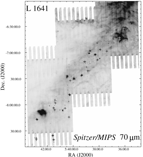
Figure 1: Spitzer/MIPS 70 $\mu$m map of L 1641. Crosses indicate the sample targets.

Figure 2: Continuum-normalised spectra, EFOSC and SofI Z band. Labels indicate the most prominent spectral features.

Figure 3: Continuum-normalised spectra, SofI J, H, and K bands. Labels indicate the most prominent spectral features.

4.2 Optical and NIR spectra

Optical and NIR continuum-normalised spectra of the sample are shown in Figures 2 and 3. The most prominent features observed in the spectra are emission lines, which have been indicated in the figures. The fluxes of the main lines, used for the analysis in this paper, are reported in Tables 4 and 4, along with the statistics on the detections. A complete list of all the detected lines in each spectrum, including fluxes, full width half maximum ($FWHM$), and equivalent widths ($W_{\lambda}$), is given in Appendix A (Tables LABEL:tab:ctf29–LABEL:tab:ctf245B1). The equivalent widths and line fluxes were calculated by integrating across the line, after subtracting the continuum, which was estimated by interpolating between two line-free adjacent regions.

The detected lines are circumstellar features and are mostly associated with YSO accretion activity or inner winds, as, e. g., H i, Ca ii, He i (see, e. g., Muzerolle et al., 1998; Natta et al., 2004; Edwards et al., 2003; Antoniucci et al., 2008), or ejection activity, as, e. g., [O i], [S ii], [Fe ii], H₂ (see, e. g., Hartigan et al., 1995; Nisini et al., 2002; Caratti o Garatti et al., 2006). A few YSOs, namely # 2, # 3, # 11, and # 18, also show permitted ionic emission lines (e. g., O i, Fe i, Fe ii, Na i, Mg ii, C i), which are characteristic of active young stars (see, e. g., Hamann & Persson, 1992a, b; Kelly et al., 1994; Hernández et al., 2004), and usually associated with chromospheric activity. In particular, the Fe i, and Fe ii emission lines have been observed in several young eruptive stars during their outburst activity (e. g. V1647 Ori, see, e. g., Fedele et al., 2007), or in YSOs showing high mass-accretion rates (e. g., Rossi et al., 1999).

The most commonly detected features are from H i recombination lines, H$\alpha$ in the optical spectra (11 out of 14, i. e. 79% detection rate), Paschen lines between 0.8 and 1.3 $\mu$m (e. g. Pa$\beta$ has a 69% detection rate - 10 out of 16), and Brackett lines between 1.5 and 2.2 $\mu$m (Br$\gamma$ has a 96% of detection rate - 26 out of 27). Other prominent bright emission lines are the Ca ii triplet between 0.85 and 0.87 $\mu$m (detected in 57% of the optical spectra), and the He i line at 1.08 $\mu$m (56% detection rate), which notably displays a clear P Cygni profile in four out of nine detections (namely source # 9, 10, 15, 18), usually indicative of inner winds in accretion disc systems (see, e. g., Edwards et al., 2003), with radial velocities larger than 300 km s^-1. Source # 2, namely [CTF93]50, only shows the blue-shifted He i line in absorption, and no indication of emission. Connelley & Greene (2010) suggest that this particular feature may be indicative of FU Orionis like stars, and might have a disc wind origin. According to Fang et al. (2009), the optical spectrum of [CTF93]50 (their source # 105) resembles those of FU Ori-like YSOs, however the typical absorption features of the CO band-head lines longward of 2.29 $\mu$m, also characteristic of FU-Ori objects, are not detected in our NIR spectrum.

Lines tracing the jet activity have also been identified in our sample, but with a detection rate lower than that of the accretion lines. Namely the [O i] line at 0.63 $\mu$m has been identified in 43% of the optical spectra, the [S ii] doublet at 0.68 $\mu$m in 36%, the [Fe ii] 1.64 $\mu$m and H₂ 2.12 $\mu$m lines in 19% and 32% of the NIR spectra, respectively. In total, jet-tracer emission lines have been observed in 14 out of 27 spectra, i. e. in 52% of the sample.

Our low resolution spectra mostly lack absorption lines on the photospheric continuum, also indicating the presence of veiling. Source # 7 and # 16 are an exception, and clearly show H i absorption features at optical and NIR wavelengths, indicating both early spectral types and lower veiling, likely indicating a more evolved stage. On the other hand, broad-band molecular absorption features, typical of cool objects, are clearly visible in both optical (VO and TiO bands) and NIR (H₂O bands) spectra. CO overtone bands have been detected in our spectra, both in absorption (sources # 8, # 11, # 18, # 24) and emission (# 14 and # 25). The CO bandheads in emission are usually believed to originate in the inner gaseous disc (see e. g. Carr et al., 1993; Antoniucci et al., 2008), and have been observed in YSOs that display strong jets and Herbig-Haro (HH) objects (see, e. g., Davis et al., 2011), whereas the CO bandheads in absorption may originate in cooler regions, like the YSO envelope (Davies et al., 2010) or the photosphere of cool YSOs (see e. g. Rayner et al., 2009).

Table 3: Main detected emission lines: accretion tracers.

Source	H$\alpha$		Ca ii 0.854/0.866 $\mu$m		He i 1.083 $\mu$m		Pa$\delta$		Pa$\gamma$		Pa$\beta$		Br$\gamma$
ID	(F $\pm$ $\Delta$ F)10-14	EW	(F $\pm$ $\Delta$ F)10-14	EW	(F $\pm$ $\Delta$ F)10-14	EW	(F $\pm$ $\Delta$ F)10-14	EW	(F $\pm$ $\Delta$ F)10-14	EW	(F $\pm$ $\Delta$ F)10-14	EW	(F $\pm$ $\Delta$ F)10-14	EW
	erg s-1 cm-2	Å	erg s-1 cm-2	Å	erg s-1 cm-2	Å	erg s-1 cm-2	Å	erg s-1 cm-2	Å	erg s-1 cm-2	Å	erg s-1 cm-2	Å
1	13$\pm$1	-11.0	$\cdots$	$\cdots$	$\cdots$	$\cdots$	0.8$\pm$0.3	-2.0	1.1$\pm$0.3	-2.8	1.8$\pm$0.4	-4.0	3.0$\pm$0.5	-5.0
2	0.99$\pm$0.04	-7	1.8$\pm$0.2/1.6$\pm$0.2	-6.4/-5.7	$\cdots$	$\cdots$	1.1$\pm$0.2	-2.5	2.0$\pm$0.4	-3.3	4.5$\pm$0.4	-4.4	7.4$\pm$0.8	-3.3
3	1330$\pm$1	-73.2	344$\pm$5/304$\pm$5	-26.6/-23.7	95$\pm$8	-5.1	152$\pm$8	-8	283$\pm$8	-16.2	386$\pm$8	-23.2	181$\pm$8	-13.0
4	82.3$\pm$0.2	-143.1	2.3$\pm$0.4/3.1$\pm$0.4	-4/-5.5	9$\pm$2	-8.5	6$\pm$2	-5.7	8$\pm$2	-8.1	10$\pm$1	-9.2	3.3$\pm$0.8	-4.5
5	0.13$\pm$0.05	$\cdots$	0.41$\pm$0.03/0.38$\pm$0.03	-19.0/-17.5	0.33$\pm$0.08	-3.7	$\cdots$	$\cdots$	0.89$\pm$0.08	-9.5	2.8$\pm$0.1	-12.7	3.8$\pm$0.4	-7.6
6	$\cdots$	$\cdots$	$\cdots$	$\cdots$	$\cdots$	$\cdots$	$\cdots$	$\cdots$	$\cdots$	$\cdots$	$\cdots$	$\cdots$	0.4$\pm$0.1	-6.5
7	18$\pm$1	-6.3	$\cdots$	$\cdots$	$\cdots$	$\cdots$	$\cdots$	$\cdots$	$\cdots$	$\cdots$	$\cdots$	$\cdots$	12$\pm$3	-3.1
8	$\cdots$	$\cdots$	$\cdots$	$\cdots$	$\cdots$	$\cdots$	$\cdots$	$\cdots$	$\cdots$	$\cdots$	$\cdots$	$\cdots$	140$\pm$10	-3.6
9	13.4$\pm$0.2	-17	$\cdots$	$\cdots$	3.8$\pm$0.8	-1.9	$\cdots$	$\cdots$	$\cdots$	$\cdots$	42$\pm$1	-1.6	10$\pm$1	-3.8
10	3.05$\pm$0.03	-96.1	1.2$\pm$0.1/1.1$\pm$0.1	-18.6/-14.1	0.89$\pm$0.08	-4.5	0.5$\pm$0.1	-3.3	1.3$\pm$0.2	-6.1	2.2$\pm$0.1	-8.5	2.2$\pm$0.4	-8.9
11	69.9$\pm$0.1	-88.2	26.4$\pm$0.4/23.0$\pm$0.4	-27.9/-24.4	28.8$\pm$0.7	-17.5	19$\pm$2	-14.7	27.0$\pm$0.8	-16.1	45$\pm$1	-21.2	30$\pm$1	-13.1
12	$\cdots$	$\cdots$	$\cdots$	$\cdots$	$\cdots$	$\cdots$	$\cdots$	$\cdots$	$\cdots$	$\cdots$	$\cdots$	$\cdots$	0.6$\pm$0.1	-4.3
13	$\cdots$	$\cdots$	$\cdots$	$\cdots$	$\cdots$	$\cdots$	$\cdots$	$\cdots$	$\cdots$	$\cdots$	$\cdots$	$\cdots$	0.2$\pm$0.1	$\cdots$
14	$\cdots$	$\cdots$	$\cdots$	$\cdots$	$\cdots$	$\cdots$	$\cdots$	$\cdots$	$\cdots$	$\cdots$	$\cdots$	$\cdots$	3.0$\pm$0.3	-11.1
15	5.18$\pm$0.05	-95.6	1.35$\pm$0.4/1.06$\pm$0.6	-21.1/-16.5	1.1$\pm$0.1	-8.7	0.5$\pm$0.1	-5.5	1.2$\pm$0.1	-9.5	2.0$\pm$0.2	-10.0	2.5$\pm$0.4	-7.2
16	$\cdots$	$\cdots$	$\cdots$	$\cdots$	$\cdots$	$\cdots$	$\cdots$	$\cdots$	$\cdots$	$\cdots$	$\cdots$	$\cdots$	7$\pm$1	-2.5
17	$\cdots$	$\cdots$	$\cdots$	$\cdots$	$\cdots$	$\cdots$	$\cdots$	$\cdots$	$\cdots$	$\cdots$	$\cdots$	$\cdots$	1.8$\pm$0.3	-6.9
18	403.0$\pm$0.5	-102.9	42.2$\pm$0.6/35.8$\pm$0.6	-44/-36	21.5$\pm$1	-9.7	29$\pm$1	-13.1	38$\pm$1	-17.6	45$\pm$1	-25.2	14.1$\pm$0.5	-16.5
19	$\cdots$	$\cdots$	$\cdots$	$\cdots$	$\cdots$	$\cdots$	$\cdots$	$\cdots$	$\cdots$	$\cdots$	$\cdots$	$\cdots$	0.3$\pm$0.1	-9.8
20	$\cdots$	$\cdots$	$\cdots$	$\cdots$	$\cdots$	$\cdots$	$\cdots$	$\cdots$	$\cdots$	$\cdots$	$\cdots$	$\cdots$	2.7$\pm$0.4	-7.1
21	$\cdots$	$\cdots$	$\cdots$	$\cdots$	$\cdots$	$\cdots$	$\cdots$	$\cdots$	$\cdots$	$\cdots$	$\cdots$	$\cdots$	0.7$\pm$0.1	-7.3
22	$\cdots$	$\cdots$	$\cdots$	$\cdots$	$\cdots$	$\cdots$	$\cdots$	$\cdots$	$\cdots$	$\cdots$	$\cdots$	$\cdots$	$<$0.1	$\cdots$
23	$\cdots$	$\cdots$	$\cdots$	$\cdots$	$\cdots$	$\cdots$	$\cdots$	$\cdots$	$\cdots$	$\cdots$	$\cdots$	$\cdots$	3.8$\pm$0.9	-5.0
24	$\cdots$	$\cdots$	$\cdots$	$\cdots$	$\cdots$	$\cdots$	$\cdots$	$\cdots$	$\cdots$	$\cdots$	$\cdots$	$\cdots$	1.74$\pm$0.08	-12.4
25	$\cdots$	$\cdots$	$\cdots$	$\cdots$	$\cdots$	$\cdots$	$\cdots$	$\cdots$	$\cdots$	$\cdots$	$\cdots$	$\cdots$	10$\pm$2	-3.6
26	$\cdots$	$\cdots$	$\cdots$	$\cdots$	0.40$\pm$0.09	-3.9	0.2$\pm$0.1	-3.8	0.4$\pm$0.1	-4.0	1.5$\pm$0.2	-5.5	4.1$\pm$0.6	-5.2
27	$\cdots$	$\cdots$	$\cdots$	$\cdots$	$\cdots$	$\cdots$	$\cdots$	$\cdots$	$\cdots$	$\cdots$	$\cdots$	$\cdots$	1.6$\pm$0.8	-11.1
Detections	11/14 - 79%		8/14 - 57%		9/16 - 56%		9/16 - 56%		10/16 - 62%		11/16 - 69%		26/27 - 96%

Table 4: Main detected emission lines: ejection tracers.

Source	[O i] 0.630 $\mu$m		[S ii] 0.672/3 $\mu$m		[Fe ii] 1.644 $\mu$m		H2 2.122 $\mu$m
ID	(F $\pm$ $\Delta$ F)10-14	EW	(F $\pm$ $\Delta$ F)10-14	EW	(F $\pm$ $\Delta$ F)10-14	EW	(F $\pm$ $\Delta$ F)10-14	EW
	erg s-1 cm-2	Å	erg s-2.3-1 cm-2	Å	erg s-1 cm-2	Å	erg s-1 cm-2	Å
2	0.77$\pm$0.02	-7.1	0.33$\pm$0.03/0.55$\pm$0.03	-2.1/-3.4	2.1$\pm$0.8	-1.1	$\cdots$	$\cdots$
4	1.3$\pm$0.1	-2.7	$\cdots$	$\cdots$	$\cdots$	$\cdots$	$\cdots$	$\cdots$
5	$\cdots$	$\cdots$	$\cdots$	$\cdots$	2.9$\pm$0.2	-1.9	1.4$\pm$0.4	-2.8
6	$\cdots$	$\cdots$	$\cdots$	$\cdots$	$\cdots$	$\cdots$	0.2$\pm$0.1	-5.4
9	$\cdots$	$\cdots$	$\cdots$	$\cdots$	$\cdots$	$\cdots$	3$\pm$1	-1.3
10	0.26$\pm$0.02	-17.2	0.07$\pm$0.03a/0.09$\pm$0.03	-2.6/-3.1	$\cdots$	$\cdots$	0.9$\pm$0.4	-3.5
11	2.0$\pm$0.1	-3.1	0.4$\pm$0.1	-0.5	$\cdots$	$\cdots$	$\cdots$	$\cdots$
12	$\cdots$	$\cdots$	$\cdots$	$\cdots$	$\cdots$	$\cdots$	0.7$\pm$0.1	-4.3
14	$\cdots$	$\cdots$	$\cdots$	$\cdots$	0.57$\pm$0.07	-6.6	$\cdots$	$\cdots$
15	0.54$\pm$0.05	-12.6	0.26$\pm$0.04/0.32$\pm$0.04	-4.5/-5.5	$\cdots$	$\cdots$	0.8$\pm$0.2	-2.5
18	9.1$\pm$0.4	-2.6	1.5$\pm$0.4/3.0$\pm$0.4	-0.4/-0.8	4$\pm$1	-3.2	$\cdots$	$\cdots$
22	$\cdots$	$\cdots$	$\cdots$	$\cdots$	$\cdots$	$\cdots$	0.2$\pm$0.1	-2.8
24	$\cdots$	$\cdots$	$\cdots$	$\cdots$	2.48$\pm$0.05	-45.8	0.7 $\pm$0.06	-4.9
Detections	6/14 - 43%		5/14 - 36%		5/27 - 19%		8/27 - 30%

4.3 Spitzer IRS spectra

Our IRS Spitzer spectra are shown in Figure 4. The flux densities for the Y-axes have been scaled and shifted for a better display. Moreover, the three panels have a different Y-axis range to properly fit the different steepness of the spectra. Such a variety already shows that the SED spectral index of our YSOs has a spread larger than originally expected (see Sect. 2), i. e. $\alpha>-1$, instead of $\alpha>-0.4$, as we will see later in Sect. 4.4.2.

There are a few emission features detected in the Spitzer spectra, mostly H₂ pure rotational lines (at 17.0 and 28.2 $\mu$m) (detected in 50%, i. e. 10/20), [Fe ii] (at 17.9, 22.9, 24.5, and 35.8 $\mu$m) (detected in 40%, i. e. 8/20), [Si ii] and [Si iii] (at 34.8 and 35.3 $\mu$m, and at 25.6 $\mu$m) (detected in 50% and 55%, respectively, i. e. 10/20 and 11/20), and [S iii] (at 33.5 $\mu$m) (detected in 65%, i. e. 13/20). There are also a few lines which we tentatively assign to [Fe i] (at 24, 28.5, and 36.5 $\mu$m) (detected in 30%, i. e. 6/20). These lines are quite common in Mid-IR YSO spectra (see, e. g., Forbrich et al., 2010; Lahuis et al., 2010; Baldovin-Saavedra et al., 2011), and mostly originate from both dissociative (e. g. [S iii], [Si ii], [Si iii], [Fe ii], [Fe i]) and non-dissociative (H₂) shocks along the YSOs jets (Lahuis et al., 2010), whereas a few lines may also originate from the discs, as H₂, [Si ii], [Si iii], [Fe i] (see, e. g., Lahuis et al., 2007). A complete list of all the detected lines is given in Appendix A (Tables LABEL:tab:ctf29-LABEL:tab:ctf245B1).

Several YSOs in our sample show prominent ice absorption features at 5–8 $\mu$m (H₂O) and 15.2 $\mu$m (CO₂) (79% of the sample) as well as the amorphous silicate absorption feature at 9.7 $\mu$m (observed in all the IRS Spitzer spectra). This last feature is detected in absorption in all sources except #7 and #18, where it is observed in emission, usually indicating more evolved objects (see, e. g., Watson et al., 2004). These broadband features are usually connected to dust and ice mantels on dust in the interstellar medium and in the YSO envelope, and their optical depths have been used in several works to compute extinction towards the protostellar photospheres (see, e. g., Alexander et al., 2003; Chiar et al., 2007).

Figure 4: Spitzer IRS spectra. Flux densities have been shifted and normalised by a constant value for a better display. Labels indicate the detected spectral features.

4.4 Derived stellar parameters

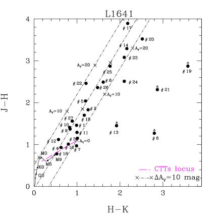
Figure 5: Top panel: $JH$ vs. $HK$ diagram for our L1641 targets. Dwarf MS and classical T Tauri loci (Meyer et al., 1997) are indicated by a continuous black line and a dashed magenta line, respectively. Black dotted dashed lines show the reddening vectors. Bottom panel: IRAC colour-colour diagram for the L1641 targets. The black dotted dashed rectangle delineates the domain of Class II YSOs (Allen et al., 2004), two parallel lines indicate the locus of reddened Class II sources (Megeath et al., 2004), and an average reddening vector for $A_{\mathrm{V}}$=30 mag is plotted, as well.

4.4.1 Reddening

To obtain correct estimates of important stellar parameters, such as the accretion luminosity ($L_{acc}$), bolometric and stellar luminosities ($L_{bol}$ and $L_{*}$), mass accretion and mass ejection rates ($\dot{M}_{acc}$, and $\dot{M}_{out}$), the observed line fluxes and photometry must be properly dereddened. Thus, deriving an accurate value of the visual extinction ($A_{\mathrm{V}}$) towards the stellar photosphere and its circumstellar region is a fundamental task. There are several independent methods to compute $A_{\mathrm{V}}$, and they are successfully applied to CTTs, that are usually less embedded. Determining the extinction towards more embedded protostars is particularly difficult, however, due to the high extinction and/or scattered light from the outflow cavities and reflection nebulae surrounding the YSOs (see, e. g., Whitney et al., 2003b; Beck, 2007; Connelley & Greene, 2010).

In this work, we have combined our multi-wavelength spectroscopy and photometry to obtain independent estimates of the visual extinction (see Table 5), namely:

i) Line ratios of transitions arising from the same upper level can be used to evaluate $A_{\rm V}$. Indeed the observed ratio depends only on the differential extinction, if the emission is optically thin, and once the theoretical value, which depends on the Einstein coefficients and frequencies of the transitions, is known.

We use the Br$\gamma$ to Pa$\delta$ ratio, assuming that the observed emission arises from optically thin gas. Results are reported in column 2 of Tab. 5. [Fe ii] line ratios are also used, in particular 1.644/1.257 $\mu$m (source #2, #5, and #18), 1.644/1.321 $\mu$m (source #5) or 1.71/1.60 $\mu$m (source #24), adopting the transition probabilities of Nussbaumer & Storey (1988). Results are reported in column 3 of Tab. 5.

ii) The optical depth of the 9.7 $\mu$m amorphous silicate absorption feature ($\tau_{9.7}$) and optical depth of the CO₂ ice feature at 15.2 $\mu$m ($\tau_{15.2}$) can also be used to estimate the extinction.

To measure the optical depths, the following steps were followed. First we determined the stellar continuum by fitting a low-order polynomial on a log-log scale to the spectral segments between 5 and 35 $\mu$m, which are not affected by absorption features (see e. g. Boogert et al., 2008). Then, we applied to derive $\tau_{\lambda}$, the following relationship (see, e. g., Alexander et al., 2003; Chiar et al., 2007):

$$\tau_{\lambda}=-ln(F_{source}(\lambda)/F_{cont}(\lambda))$$ (1)

where $F_{source}$ and $F_{continuum}$ are the flux densities of the source and of the continuum fit at $\lambda$, respectively. $\tau_{\lambda}$(CO₂)_ice can be converted to a column density, using the following relationship (see, e. g., Alexander et al., 2003):

$$N(CO_{2})=\frac{\int{\tau_{\lambda}d\lambda}}{\lambda^{2}_{peak}A}$$ (2)

where $\int{\tau_{\lambda}d\lambda}$ is the equivalent width, $\lambda_{peak}$ is the wavelength of the feature peak optical depth, and $A$ is the ice band strength ($1.1\times 10^{–17}$ cm molecule^-1) assuming pure CO₂ ice (Gerakines et al., 1995; Alexander et al., 2003).

The $A_{\mathrm{V}}$ value for the silicates is obtained from Rieke & Lebofsky (1985) as $A_{\mathrm{V}}$= $\tau_{9.7}\times 18$, and from the CO₂ column density using the relationships of  Bergin et al. (2005). Results from the CO₂ and silicate measurements are reported in Columns 4 and 5 of Tab. 5, respectively.

iii) Colour-colour diagrams from $J-$, $H-$, and $K-$band $2MASS$ photometry. Fig. 5 (top panel) shows the $J-H$ vs $H-K$ colours of our targets, along with the dwarf-MS and CTTs loci (Meyer et al., 1997), and the reddening vectors. Many of the sources are located along the reddening band extending from the CTTs locus, while there are a few objects positioned on the right side of the strip, indicating less evolved objects. Arrows on these objects indicate lower limits, because their $J-$band magnitude is an upper limit or has a S/N ratio $\leq$3. Derived $A_{\mathrm{V}}$ values are reported in column 6 of Tab. 5.

iv) Self-consistent method (SCM, see Sect. 4.4.5 and Antoniucci et al., 2008, for a detailed description). This method relies on the fact that there are two ways of determining the source stellar luminosity $L_{*}$, both depending on the actual extinction value: i) from the bolometric luminosity $L_{bol}$ (see Sect. 4.4.2) and the accretion luminosity $L_{acc}$ derived from the de-reddened Pa$\beta$ (and/or Br$\gamma$) flux (Sect. 4.4.3), assuming that $L_{*}=L_{bol}-L_{acc}$; ii) from the observed $K$ band magnitude of the source, considering the distance, the spectral type, and an estimate of the veiling in the relevant band (see Sect. 4.4.4). An average veiling value of $r_{K}$ = 1 for the whole sample is assumed. Because veiling dependence on magnitude is logarithmic, while extinction dependence is linear, the computation is less sensitive to veiling variations. For example, assuming $r_{K}$ = 5, instead of one, would increase $A_{\mathrm{K}}$ of $\sim$0.48, i. e. $\sim$5 mag in the $V$ band.

The best estimate of the extinction will be the one for which we obtain the same value of $L_{*}$ from both computations.

For comparison, additional extinction estimates retrieved from the literature (Strom et al., 1989; Fang et al., 2009; Connelley & Greene, 2010) are also reported in column 8 of Tab. 5.

The inferred $A_{\mathrm{V}}$ values range from 0 to $\sim$30 mag, although the different methods adopted here usually produce a wide range of results for each object. Indeed this is a well known problem for Class I sources (see e. g. Beck, 2007; Prato et al., 2009; Davis et al., 2011), and it is due to several reasons, as e. g.: i) the considered lines trace different regions of the YSO (e. g., the circumstellar region or the jet, the H i or the [Fe ii] lines, respectively), possibly with different extinctions; ii) scattering is not taken into account by any of the above methods, although those based on the [Fe ii] line ratios or on MIR optical depths should not be significantly affected; iii) a standard ISM law (Rieke & Lebofsky, 1985) has been assumed to correct for the differential extinction, without considering that it can vary, depending on the size and properties of the grains in the disc, envelope, or jet (see, e. g. Cardelli et al., 1989).

Despite these limitations, Tab. 5 shows a relatively good agreement among the different methods. In particular, the cross correlation coefficient between different sets of $A_{\mathrm{V}}$ ranges between $r=0.95$ (Si vs SCM) with an rms of $\sim$3 mag, to $r=0.66$ (CC vs SCM) with an rms of $\sim$6 mag. The average value is $r=0.86$. We then adopt an average $A_{\mathrm{V}}$ value for each object (column 9 of Tab. 5), after discarding those that deviate from the average by more than one sigma.

Table 5: Visual extinction values of the sample.

Source	$A_{\mathrm{V}}$(HI)	$A_{\mathrm{V}}$([Fe ii])	$A_{\mathrm{V}}$(CO2)	$A_{\mathrm{V}}$(Si)	$A_{\mathrm{V}}$-CC	$A_{\mathrm{V}}$-SCM	$A_{\mathrm{V}}$ pub	$A_{\mathrm{V}}$-adp
ID	(mag)	(mag)	(mag)	(mag)	(mag)	(mag)	(mag)	(mag)
1	8$\pm$3	$\cdots$	$\cdots$	1-2	4$\pm$0.5	1	4.22	2
2	9.5$\pm$1	5$\pm$5	11	8-9	8$\pm$0.5	8.6	91; 62	8.5
3	3.7$\pm$0.5	$\cdots$	$\cdots$	$\cdots$	2$\pm$0.4	0	1.7–91	2
4	1$\pm$0.5	$\cdots$	$\cdots$	3-6	1.5$\pm$0.6	4	0.21; 5.72	3
5	$\cdots$	11$\pm$4	6-9	5-7	10.5$\pm$0.4	9	121	10
6	$\cdots$	$\cdots$	25-30	20-22	$>$14	24	$\cdots$	24
7	$\cdots$	$\cdots$	$\cdots$	$<$1	0$\pm$0.5	0	91; 6$\pm^{(1.6)}_{(0.6)}\,{}^{3}$	0
8	$\cdots$	$\cdots$	$\cdots$	$\cdots$	19$\pm$0.5	$\cdots$	191	19
9	$\cdots$	$\cdots$	3	$\cdots$	4.5$\pm$0.4	1	4.71	2
10	8.3$\pm$1.2	$\cdots$	$\cdots$	5-7.2	6$\pm$0.5	11	$\cdots$	8.2
11	4.6$\pm$0.5	$\cdots$	$\cdots$	$\cdots$	2.5$\pm$0.5	1.5	71	2
12	$\cdots$	$\cdots$	$\cdots$	$\cdots$	4$\pm$1	12	$\cdots$	8
13	$\cdots$	$\cdots$	22-25	12-18	$>$8	36	$\cdots$	25
14	$\cdots$	$\cdots$	21-27	22-30	22$\pm$2	24	281; 25.43	24
15	8.7$\pm$0.7	$\cdots$	9.5	4.5-6.5	7.5$\pm$0.5	8	131; 5.82	8.5
16	$\cdots$	$\cdots$	4.5	3-6	2$\pm$0.4	$\cdots$	4.41; 6.72	4
17	$\cdots$	$\cdots$	23-26	11-15	28$\pm$2	16	201	23
18	0.5$\pm$0.5	3$\pm$2	4.5	1-2	0$\pm$0.4	2	51; 2.62	2
19	$\cdots$	$\cdots$	25	13-15	21$\pm$4	22	$\cdots$	20
20	$\cdots$	$\cdots$	25-32	14-20	23$\pm$4	13	261	23
21	$\cdots$	$\cdots$	20-35	17-20	$>$16	21	$>$4.53	22.5
22	$\cdots$	$\cdots$	$\cdots$	$\cdots$	14$\pm$2	10	$\cdots$	12
23	$\cdots$	$\cdots$	21	18-25	19$\pm$2	24	161	21
24	$\cdots$	20$\pm$10	$\cdots$	25-30	16$\pm$2	26	341; 13-243	25
25	$\cdots$	$\cdots$	26-30	14-16	18.5$\pm$2	16	$\cdots$	18
26	11.3$\pm$5	$\cdots$	$\cdots$	$\cdots$	13.0$\pm$0.5	6	$\cdots$	10
27	$\cdots$	$\cdots$	$\cdots$	$\cdots$	7.5$\pm$0.5	8	6.31	8

¹ Strom et al. (1989); ² Fang et al. (2009); ³ Connelley & Greene (2010).

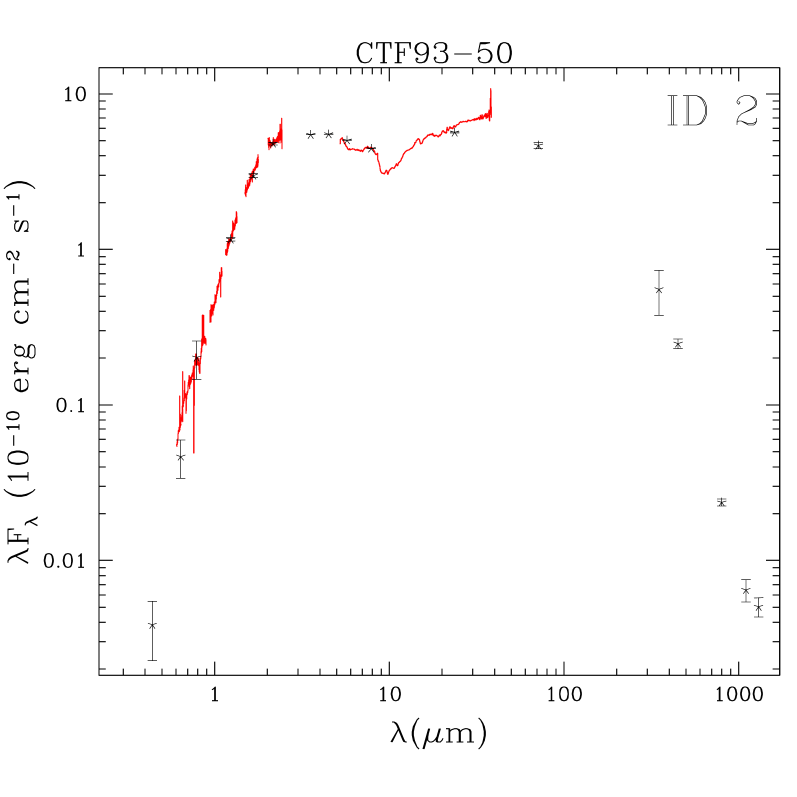
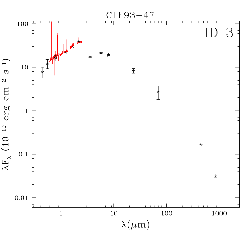
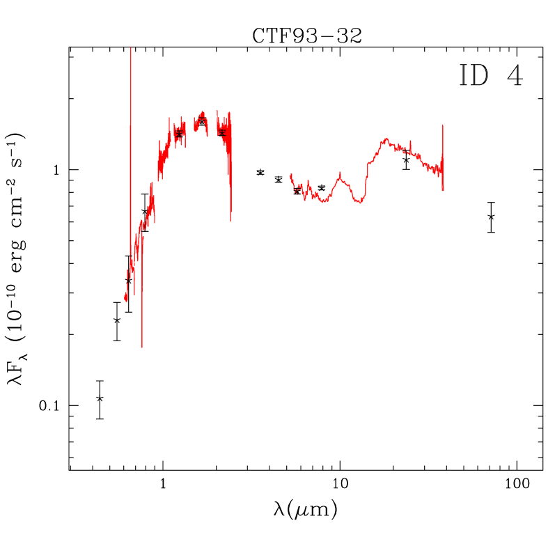
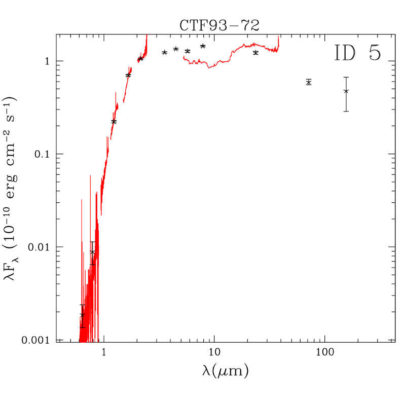
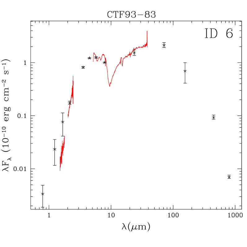
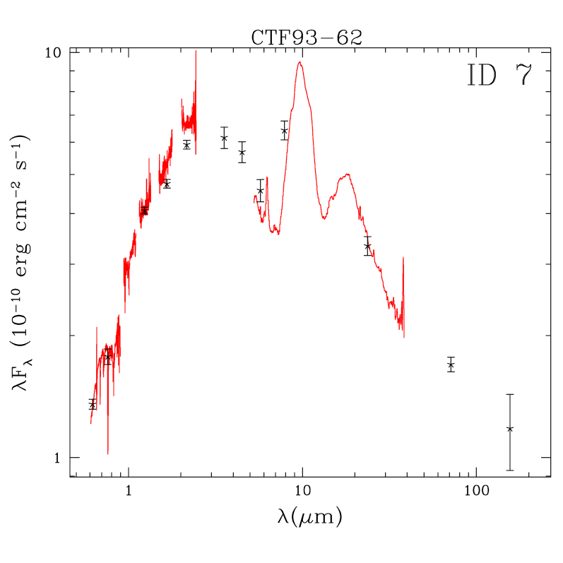
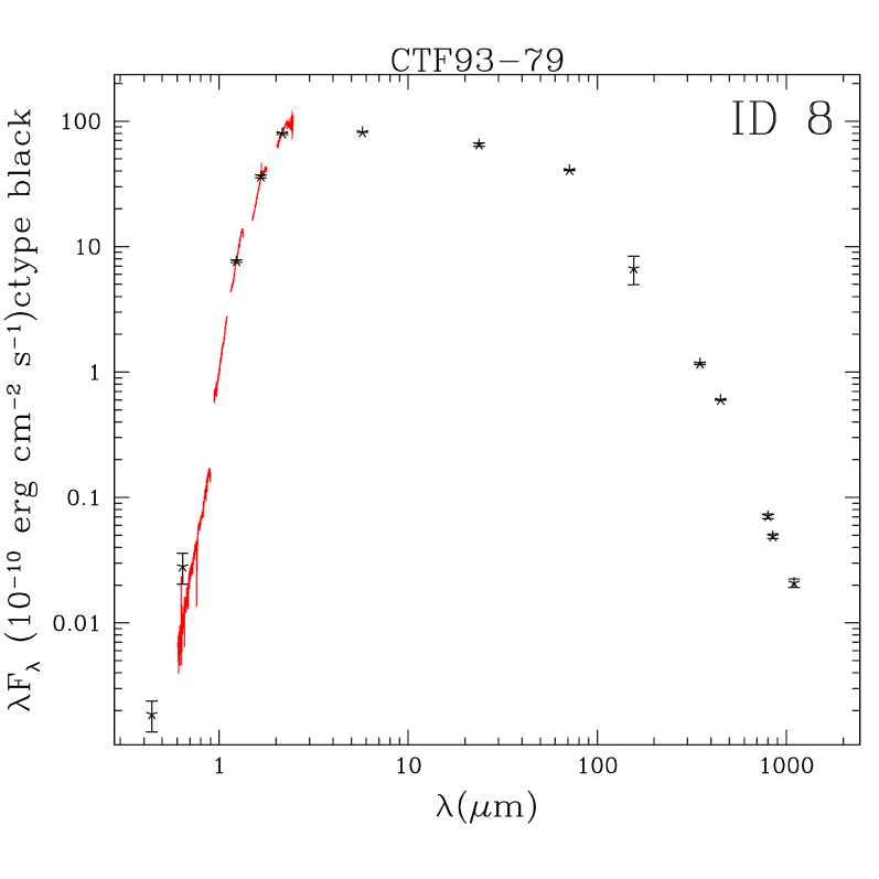
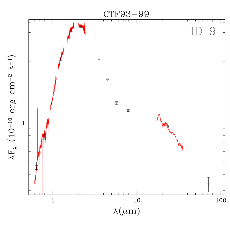
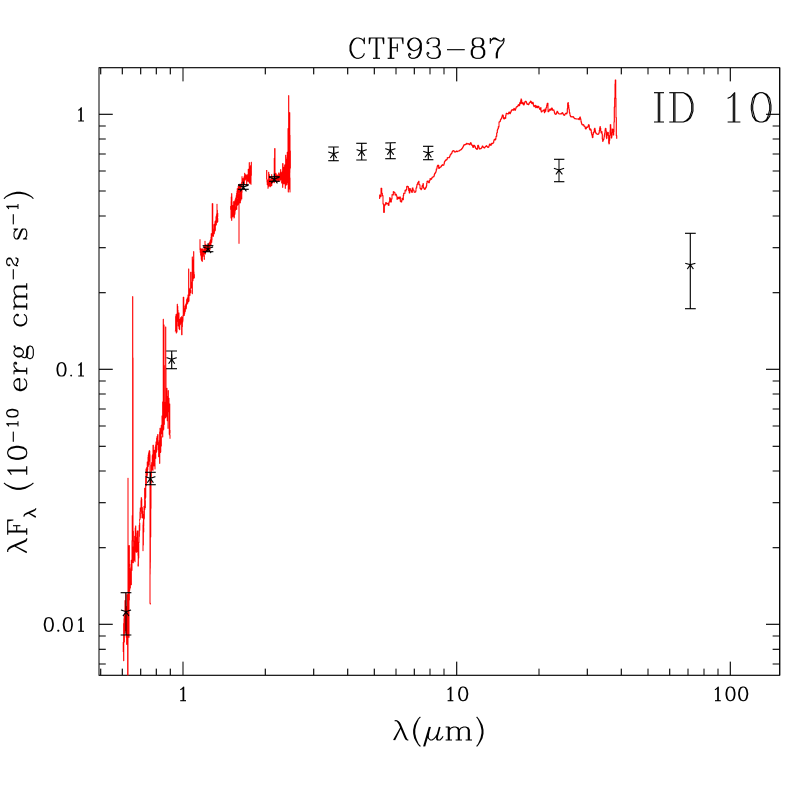
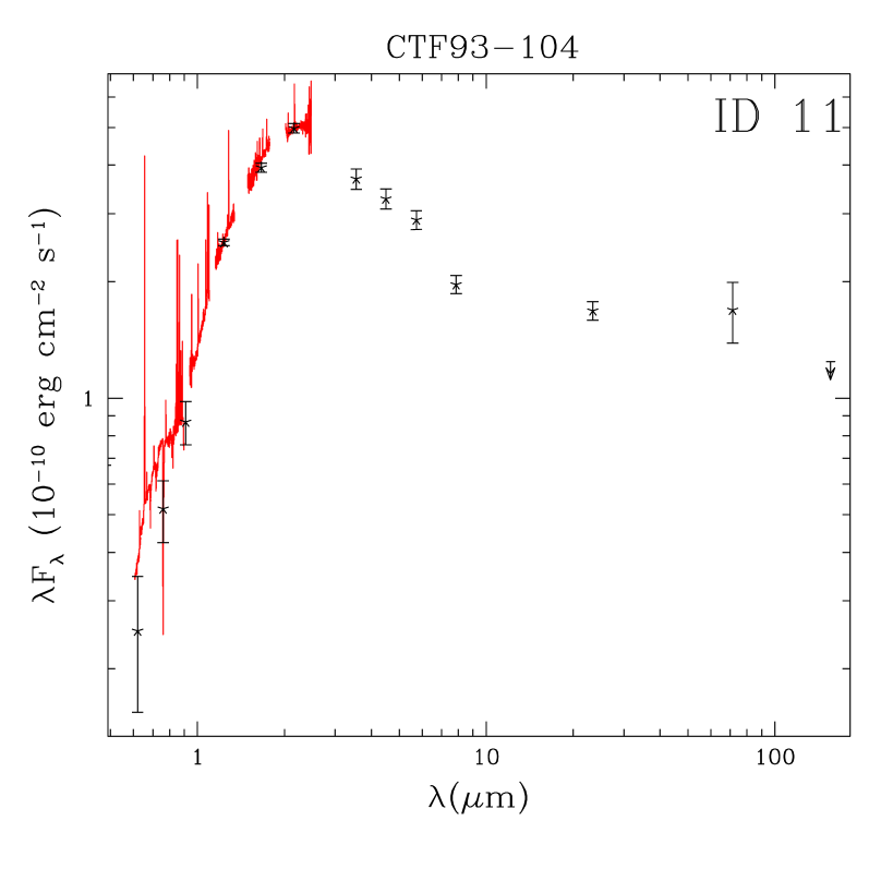
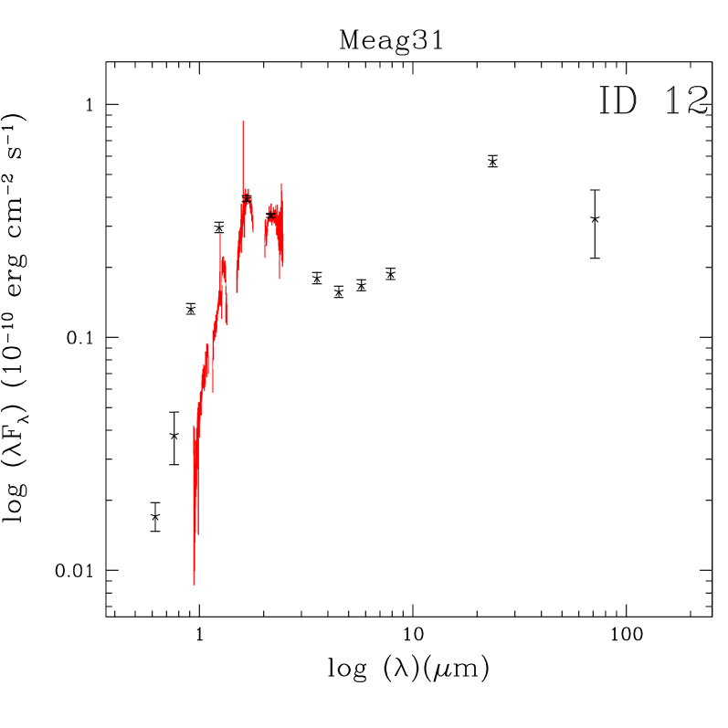
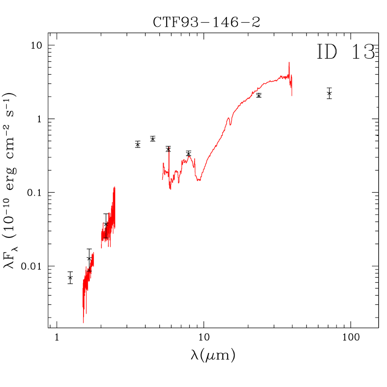
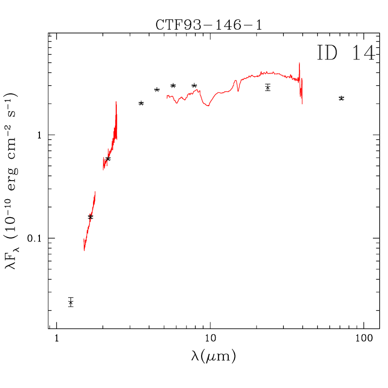
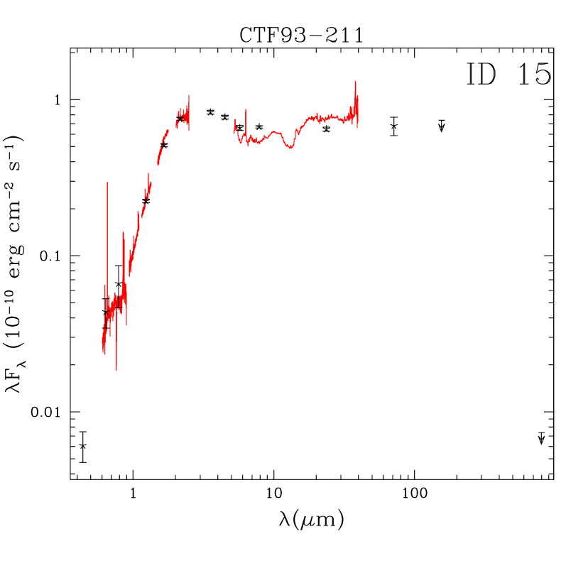
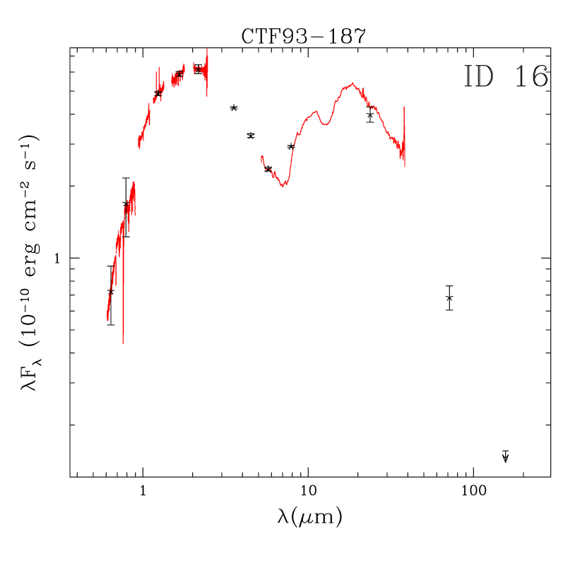
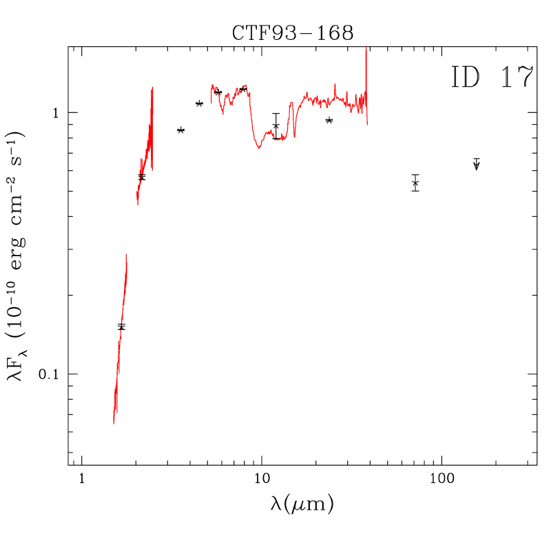
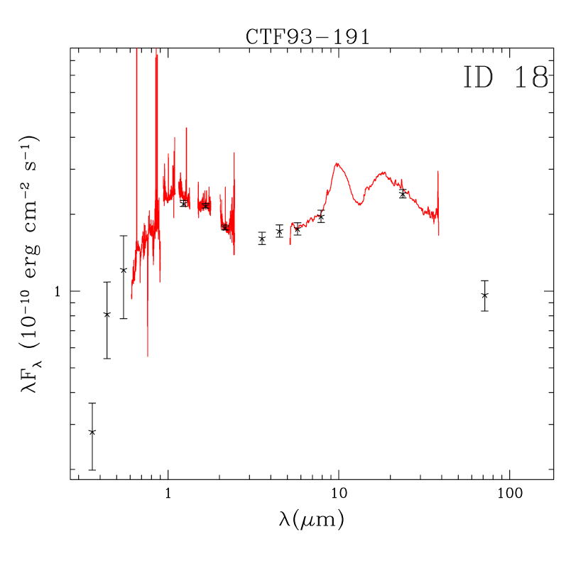
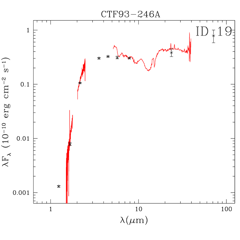
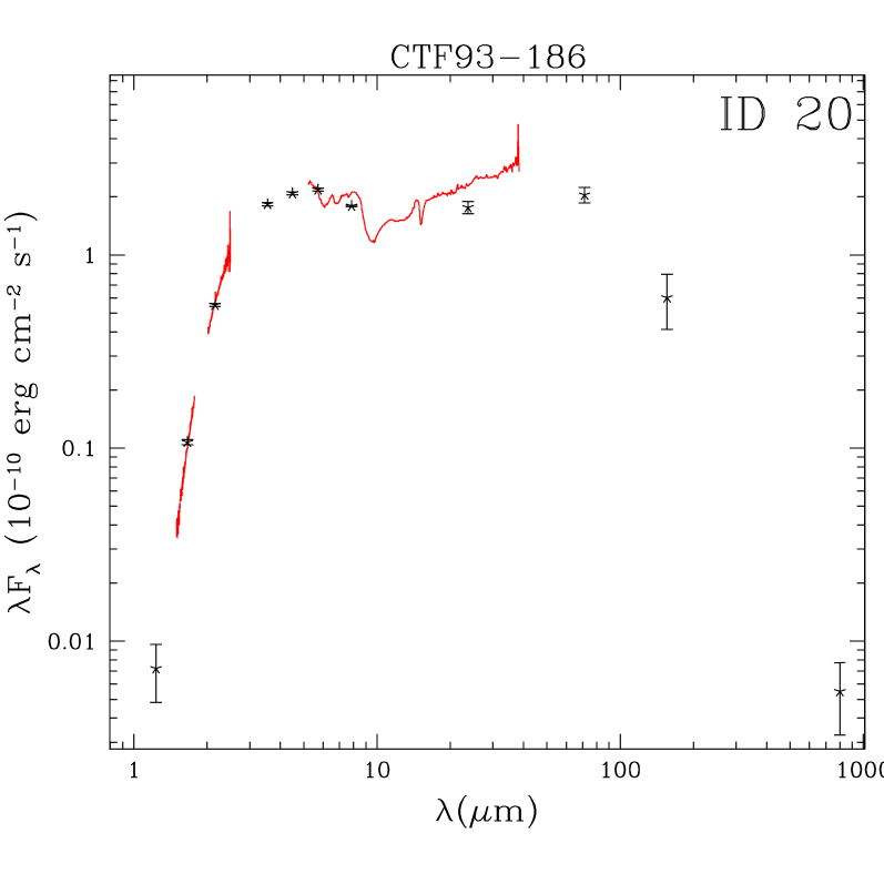
Figure 6: Target SEDs and spectra. Photometric data with error bars are in black, spectroscopic data (ESO-NTT and Spitzer) are in red. Target IDs and names are also reported. - to be continued

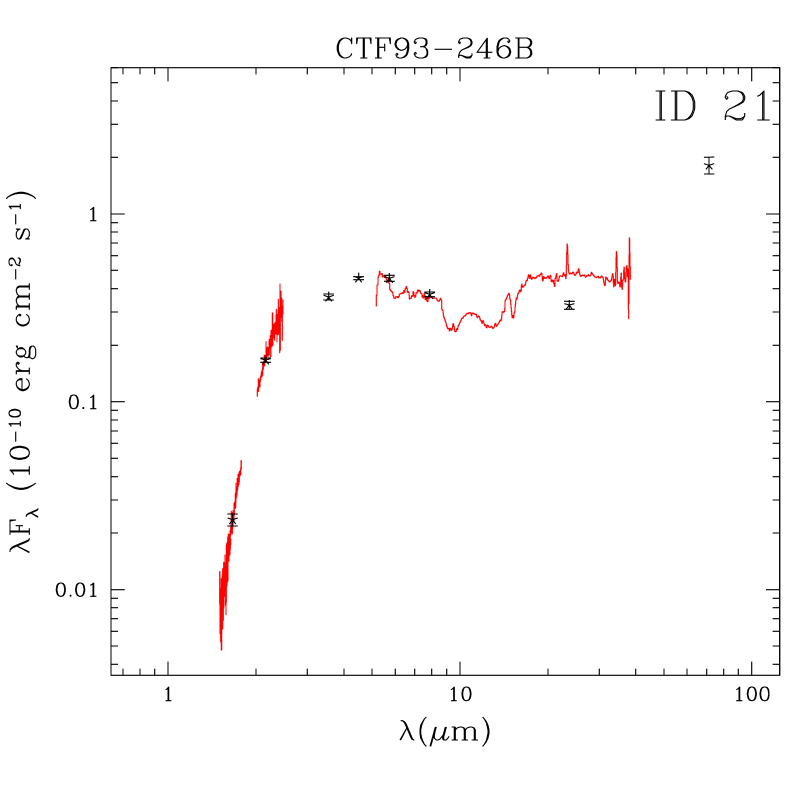
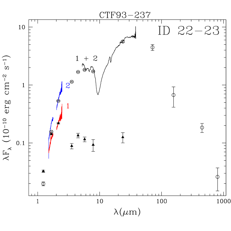
Figure 6: Target SEDs and spectra. Photometric data with error bars are in black, spectroscopic data (ESO-NTT and Spitzer) are in red. Target IDs and names are also reported. - continued

4.4.2 SEDs and $L_{bol}$

Both photometric and spectroscopic data of our sources are incorporated in the SEDs presented in Figure 6, where both target IDs and names are also reported. In general, there is an excellent agreement between observed optical-IR spectra and photometric points, independently obtained from images. However, there is a marginal discrepancy between the two datasets for a few objects, especially at short wavelengths (see, e. g., source # 6, # 13, # 19), which is likely due to scattering effects, and/or intrinsic YSO variability. Mismatches between Spitzer spectra and photometry are also observed in a few sources (see, e. g., # 5, # 10, # 14), and might be due to variability, as already observed in the literature (see, e. g., Morales-Calderón et al., 2009). Special mention is needed of source # 25 (or [CTF93]216-2), which underwent a strong outburst between 2007 and 2008 (Caratti o Garatti et al., 2011), increasing in brightness by $\sim$4.6, 4.0, 3.8, and 1.9 mag in the $J$, $H$, $K_{s}$ bands and at 24 $\mu$m. The panel in Figure 6 shows both pre- and outburst SEDs. Photometric pre-outburst and outburst values are reported in Tab. 10 and in Caratti o Garatti et al. (2011), respectively.

The YSO Class is determined from the SED slope ($\alpha$, or spectral index), which is calculated over all the available data points between 2.2 and 24 $\mu$m. The spectral index value is obtained from a linear fit to the logarithms, taking into account the uncertainties in the flux measurements. Depending on $\alpha$, our sources were classified as Class I ($\alpha\geq 0.3$), Flat spectrum ($−0.3\leq\alpha\leq 0.3$), or Class II ($−1.6\leq\alpha<−0.3$). $\alpha$ values of the sample range from 1.60 to -1.04, including 9 Class I, 11 Flat, and 7 Class II YSOs. Notably, as already observed for other outbursting sources (see, e. g., Kóspál et al., 2011, and references therein), source # 25 changed its colours and its SED slope (from 0.69 to 0.25, pre- and outburst phase, respectively). Despite its actual $\alpha$ values, in this paper we consider it as a Class I source.

The source ID, their $\alpha$ values and corresponding classifications are reported in Columns 1, 2, and 3 of Table 7, respectively. As already mentioned in Sect. 2, the $\alpha$ values (and thus the YSO classification) listed in Chen & Tokunaga (1994) often differ from ours, in some cases substantially as, e. g., for source #9 (-0.45 vs 1.1, our and their value, respectively) or for source #11 (-0.49 vs 1), indicating that IRAS fluxes should not be used for those objects located in crowded regions, as the resulting classification is not reliable.

The total bolometric luminosity ($L_{bol}$) of each source was derived by integrating the observed SED (see Figure 6), which includes data ranging from optical to mm wavelengths. The calculation was performed starting from the first available SED data point (which varies from source to source, see also Table 10), using straight line interpolation (in the $Log(\lambda)-Log(\lambda F_{\lambda})$ plot) between all the SED points, also including additional points from the observed spectra. A final correction at the longest wavelength was applied assuming that $F_{\lambda}$ decreases as $\lambda^{-2}$. A distance value of 450 pc was assumed for the entire sample (see, e. g., Allen & Davis, 2008). $L_{bol}$ inferred values for the sample range from $\sim$0.3 to 188 $L_{\sun}$, and are listed in column 4 of Table 7. For the outburst source #25, both pre- and outburst $L_{bol}$ and $\alpha$ values are reported.

It worths noting that no correction for geometrical effects has been applied to the inferred bolometric luminosities, because system inclinations are not well defined. On the other hand, SED models from Whitney et al. (2003b) indicate that, due to geometrical effects, the observed bolometric luminosities of embedded objects may differ from their intrinsic luminosities up to a factor of two between pole-on and edge-on systems. Another source of uncertainty for $L_{bol}$ may be given by the foreground extinction, which cannot be correctly estimated, because the inferred $A_{\mathrm{V}}$ values of Sect. 4.4.1 do not discriminate between foreground and circumstellar contribution. However, extinction maps can provide us with upper limits for the foreground extinction. From Rowles & Froebrich (2009) maps, we infer an average $A_{\mathrm{V}}$ value of $\sim$6 mag towards our targets, which would modify $L_{bol}$ values between 5 and 10%, because foreground extinction only affects the shortest wavelengths of the SED. As a consequence, estimates of $L_{bol}$ and other stellar parameters (i. e., $L_{*}$, $M_{*}$, $R_{*}$, age, and $\dot{M}_{acc}$), that will be later derived from it, might also be affected by such uncertainties.

4.4.3 Accretion luminosity

The accretion luminosity is the main indicator of YSO accretion activity. Many different techniques exist in the literature to derive it (see, e. g., Calvet et al., 2000), from the measurement of the U-band excess luminosity  (Gullbring et al., 1998) to the luminosity of optical and infrared emission lines (as, e. g., H$\alpha$, Ca ii, Pa$\beta$, Br$\gamma$; e. g., Muzerolle et al., 1998; Calvet et al., 2004; Natta et al., 2004, 2006), which are thought to be mainly produced in the magnetospheric accretion flow. The inferred relationships have been successfully tested for a wide range of YSO masses, from substellar-mass to intermediate-mass YSOs (Calvet et al., 2004; Natta et al., 2004; Garcia Lopez et al., 2006), but have been rarely tested simultaneously on the same YSO sample (Muzerolle et al., 1998; Rigliaco et al., 2011), because of the wide wavelength spread between the considered lines and the intrinsic YSO variability, which require simultaneous coverage of the optical and infrared spectral wavelength range.

In paper-1 we analysed various empirical line-$L_{acc}$ relationships from five different tracers, namely [O i] at 6300Å, H$\alpha$, Ca ii at 8542Å, Pa$\beta$, and Br$\gamma$, critically discussing the various determinations in the light of the source properties. As a result, we showed that the Br$\gamma$ and Pa$\beta$ lines give the smallest dispersion of $L_{acc}$ over the entire range of $L_{*}$, whereas the other tracers, especially the H$\alpha$ and [O i] lines, provide much more scattered $L_{acc}$ results, not expected for the homogeneous sample of targets observed.

Here, we use our 0.6-2.5 $\mu$m spectra to derive $L_{acc}$ simultaneously from the Ca ii, Pa$\beta$, Br$\gamma$ line luminosities.

As in paper-1, $L_{acc}$ from these lines is derived from the following empirical relationships (Herczeg & Hillenbrand, 2008; Calvet et al., 2000, 2004):

$$Log(L_{acc}/L_{\sun})=1.02\times Log(L_{CaII8542}/L_{\sun})+2.5$$ (3)

$$Log(L_{acc}/L_{\sun})=1.03\times Log(L_{Pa\beta}/L_{\sun})+2.80$$ (4)

$$Log(L_{acc}/L_{\sun})=0.90\times Log(L_{Br\gamma}/L_{\sun})+2.90$$ (5)

Line luminosities were obtained after de-reddening the observed fluxes by the adopted $A_{\mathrm{V}}$ (Table 5), using the standard  Rieke & Lebofsky (1985) extinction law, and assuming a distance of 450 pc. Results are reported in Table 6, where source ID, $L_{acc}$(Br$\gamma$), $L_{acc}$(Pa$\beta$), and $L_{acc}$(Ca ii_0.854) are listed. The derived values range from $\sim$0.1 to $\sim$60 L_☉. We assigned an upper limit to source # 23, computed from the upper limit for Br$\gamma$ emission.

In Figure 7 we compare the obtained results, plotting $Log(L_{acc}(Pa\beta))$ vs $Log(L_{acc}(Br\gamma))$ (black circles), and $Log(L_{acc}({Ca\textsc{ii}}))$ vs $Log(L_{acc}(Br\gamma))$ (red triangles). The dashed line indicates the equivalent locus. In the first case, Pa$\beta$ vs Br$\gamma$, there is a very good agreement with a correlation coefficient $r$ equal to 0.92, whereas the correlation of the second dataset (Ca ii vs Br$\gamma$) gives a worst match with $r=0.8$, as can also be noted from the larger scatter in the plot. Such a difference cannot be attributed to a wrong extinction estimate, with the possible exception of source # 11 (see also Tab. 6), otherwise, due to differential extinction, we would observe the data points below the dotted line with the circles positioned above the triangles (overestimated extinction), or the opposite (underestimated extinction). It is worth noting that our low resolution spectroscopy does not allow us to de-blend the Ca ii (0.854 $\mu$m) and the Pa 15 (0.855 $\mu$m) lines, thus the observed Ca ii flux at 0.854 $\mu$m might be overestimated up to $\sim$20%. As a consequence, we prefer to discard the values from the Ca ii lines. For each source we adopt an average $L_{acc}$ value, obtained by averaging the accretion luminosities inferred from the Br$\gamma$ and Pa$\beta$ lines. Results are reported in column 7 of Table 7.

Table 6: Accretion luminosity estimates from Br$\gamma$, Pa$\beta$, and Ca ii 0.854 $\mu$m lines.

Source	$L_{acc}$(Br$\gamma$)	$L_{acc}$(Pa$\beta$)	$L_{acc}$(Ca ii 0.854)
ID	(L☉)	(L☉)	(L☉)
1	0.6	0.2	$\cdots$
2	1.7	1.2	1.9
3	16.5	21.2	15.3
4	0.5	0.71	0.2
5	1.06	1.13	1.17
6	0.5	$\cdots$	$\cdots$
7	1.2	$\cdots$	$\cdots$
8	61.3	$\cdots$	$\cdots$
9	1.17	2.05	$\cdots$
10	0.57	0.55	1.34
11	3.23	2.21	1.00
12	0.15	$\cdots$	$\cdots$
13	0.3	$\cdots$	$\cdots$
14	3.1	$\cdots$	$\cdots$
15	0.63	0.47	1.43
16	1.0	$\cdots$	$\cdots$
17	1.78	$\cdots$	$\cdots$
18	1.70	2.44	2.11
19	0.31	$\cdots$	$\cdots$
20	2.5	$\cdots$	$\cdots$
21	0.8	$\cdots$	$\cdots$
22	$<$0.06	$\cdots$	$\cdots$
23	2.8	$\cdots$	$\cdots$
24	2.1	$\cdots$	$\cdots$
25	0.31	$\cdots$	$\cdots$
26	1.1	0.58	$\cdots$
27	0.18	$\cdots$	$\cdots$

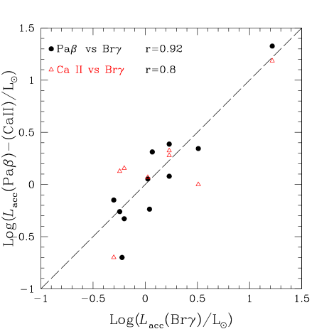
Figure 7: Comparison between the $L_{acc}$ values derived from different lines: Pa$\beta$ vs Br$\gamma$ (black circles), and Ca ii vs Br$\gamma$ (red open triangles). Correlation coefficients are also reported.

4.4.4 Stellar spectral types

We obtain the spectral types (SpTs) of our targets by combining various methods. The derived SpTs along with the method used and the effective temperatures ($T_{\rm eff}$) are reported in Table 7 (Columns 6 and 7, respectively). The adopted $T_{\rm eff}$ is converted from the spectral type adopting the relations given by Kenyon & Hartmann (1995) (for SpTs earlier than M0), and by Luhman et al. (2003) (for M0 or later SpTs).

For the 14 sources with optical spectra (see Sect. 3.1 and Tab. 1) we employ the spectral classification code SPTclass developed by Hernández et al. (2004). This code uses empirical relationships between the equivalent widths (EWs) of many atomic/molecular absorption/emission lines and $T_{\rm eff}$. As a result, this automated code can classify optical spectra to a precision of about one subtype. Additionally, spectral classifications for many of these optical sources (9 out of 14) already exist in the literature (Strom et al., 1989; Fang et al., 2009; Connelley & Greene, 2010). There is a good match ($\sim$1 subtype) with our results, except for the possible FU-Ori object [CTF93]50 (our source #2, see also Sect. 4.2), which shows a later spectral type (K6$\pm$1) with respect to previous measurements from Strom et al. (1989) (G5-G7, source KMS 31) and Fang et al. (2009) (K3-4.5, source #105 in their work). Indeed these differences are not surprising, because FU-Ori sources may show large spectral type variabilities (see e. g. Hartmann & Kenyon, 1996).

On the other hand, the thirteen remaining NIR spectra (i. e. sources # 6, 12, 13, 14, 17, 19, 20, 21, 22, 23, 24, 25, 27) show a steeply rising flat continuum that is almost featureless or with absorption water bands (in the $J$, $H$ and $K$ bands, between 1.3-1.5 $\mu$m, and 1.7-2.1 $\mu$m). These bands arise at $T_{eff}\leq$3800 K (M0 or later spectral types), and thus are typical of M type objects. Thus, these thirteen spectral types have been identified following the prescription given by Gorlova et al. (2010), i. e. dividing the spectra in two groups, which either show or do not the absorption water bands in the NIR.

H₂O broad band features are clearly detected in eight out of thirteen spectra (namely # 12, 13, 19, 21, 22, 23, 24, 25). The depth of these bands increases with decreasing temperatures, thus the values of their EWs, once corrected for the proper $A_{\mathrm{V}}$, can be related to the spectral subtype (see, e. g., Kleinmann & Hall, 1986; Greene & Lada, 1996; Luhman et al., 2003; Gorlova et al., 2010). Usually the 1.3-1.5 $\mu$m absorption feature is detected for $A_{V}<$20 mag, and the EW of the 1.7-2.1 $\mu$m feature decreases by about a factor of 2, as the visual extinction increases from 0 to 30 mag ($A_{V}$=25 mag is the maximum extinction value in our sample, see also Tab. 7, column 5). Along with the absorption water bands, source #12 (Meag31) also shows VO bands in absorption at $\sim$1.15 $\mu$m (typical of M6 or later SpTs; see, e. g., Cushing et al., 2005). On the other hand the lack of strong narrow band features, mostly due to the veiling and the low resolution of our spectra, prevents us from an accurate spectral classification. For these objects, the uncertainties on the SpT range from one to two subtypes, i. e. up to $\sim$200-300 K.

The five remaining spectra (namely sources # 6, 14, 17, 20, 27) are featureless with steeply rising SEDs, and without any sign of overturn in the $H$ or $K$ band, which means either SpT later than M0, or SpT earlier or equal to M0 and $A_{\mathrm{V}}$$>$30-40 mag (see, e. g., Greene & Lada, 1996; Gorlova et al., 2010). Our $A_{\mathrm{V}}$ estimates exclude the latter hypothesis, thus we safely classify them as K spectral types. One of them ([CTF93]245B-1, i.e. source #27) was already classified as K6 by Strom et al. (1989), thus we keep this classification. The lack of features in the remaining four sources precludes any detailed spectral analysis. Therefore, we use both our spectral and photometric data (see also Fig. 6) to model the four YSOs with the SED fitting tool from Robitaille et al. (2007) and provide some tighter constraints on the underlying stellar objects. Indeed, the SED fitting tool alone cannot confidently predict the stellar temperature in embedded sources. Even knowing the $L_{*}$ value, there is still degeneracy between $T_{*}$ and $R_{*}$ values. This degeneracy can be partially removed, given $L_{*}$, $L_{bol}$, extinction, and distance. In fact a substantial increase (decrease) of $T_{*}$ (500 K or more) produces a decrease (increase) of $R_{*}$, generating an older (younger) YSO and substantially modifying the SED shape.

Thus, as further constraints for the fitting tool, distance, extinction, and bolometric luminosity of each source were used (as listed in Tab. 7). An additional constraint is given by the YSO spectral type (K), and thus by the temperature range. Then, for each object, we obtained a grid of possible models, listed as a function of their $\chi^{2}$ values. We then select the best 50 models for each YSO, plot the output stellar temperature distribution, and infer the most likely temperature. The distribution spread gives us a rough estimate of the error. Our results are reported in Fig. 8, where, for each object, the stellar-temperature distribution (hashed histogram), normalised to its maximum, is plotted over the entire grid of models (in grey).

The derived spectral types for the entire sample are reported in Table 7 (column 6), and range from B7 to M7.5. Most of the objects ($\sim$74%) are low-mass YSOs with SpT between K5 and M7.5, four ($\sim$15%) are intermediate mass YSOs (F7 to K4), and three ($\sim$11%) are Herbig Ae/Be stars (A5 to B7).

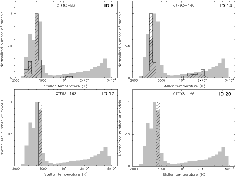
Figure 8: Temperatures inferred from SED fitting. For each YSO the stellar temperature distribution (hashed histogram), normalised to its maximum, is plotted over the entire grid of models (in grey).

4.4.5 H-R diagram and stellar parameters

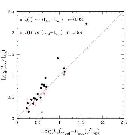
Figure 9: $L_{*}$ values derived from the $I_{J}$ and $J$ band photometry (red triangles and black dots, respectively) versus $L_{*}$ values obtained from $L_{*}=L_{bol}-L_{acc}$. The dashed line marks the equivalue locus.

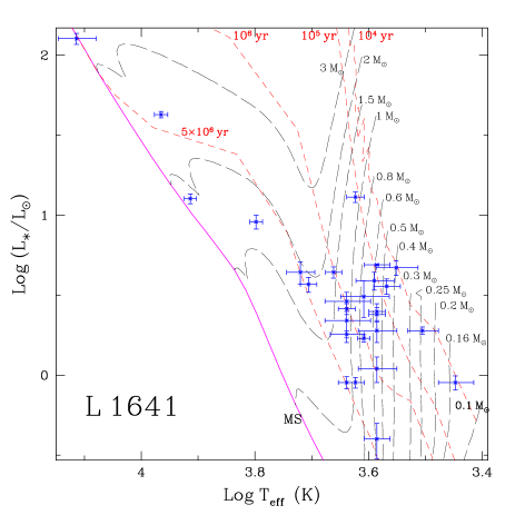
Figure 10: HR diagram for the whole sample. The evolutionary models of Siess et al. (2000) are shown with isochrones at 10⁴, 10⁵, 10⁶, and 5$\times$10⁶ yr (red dashed lines), and mass tracks from 0.1 to 3 M_☉ (black dashed lines).

Figure 11: Spectral index ($\alpha$) versus age. The two dashed lines delineate the Class I-Flat ($\alpha$ = 0.3) and Flat-Class II ($\alpha$ = -0.3) boundaries. The object IDs are also reported.

To characterise our YSOs it is necessary to derive the stellar parameters ($L_{*}$, $M_{*}$, $R_{*}$). $L_{*}$ of each source is inferred from $L_{*}=L_{bol}-L_{acc}$, i. e. assuming that the observed $L_{bol}$ is simply the sum of accretion and stellar luminosities. The resulting $L_{*}$ values are reported in Table 7 (column 8). Assuming that the YSO SED is well modelled by our data, i. e. that the derived $L_{bol}$ has a relatively small uncertainty, the error on $L_{*}$ is due to the uncertainty of the $L_{acc}$ estimates.

To test the consistency of these results we derive $L_{*}$ from the stellar bolometric magnitude (see, e. g., Gorlova et al., 2010), obtained from the dereddened $I_{J}$ and $J$ magnitudes (Table 10, Columns 5 and 6, respectively) for 22 out of 27 and 26 out of 27 objects of the sample:

$$Log(L_{*}/L_{\sun})=1.86-0.4(I-0.482A_{\mathrm{V}}+BC_{I}-5log(450)+5)$$ (6)

$$Log(L_{*}/L_{\sun})=1.86-0.4(J-0.265A_{\mathrm{V}}+BC_{J}-5log(450)+5)$$ (7)

where the bolometric correction in $I_{J}$ and $J$ ($BC_{I}$ and $BC_{J}$, respectively), for each SpT of Table 7, are inferred from the dwarf colours in Kenyon & Hartmann (1995).

Figure 9 compares in logarithmic scale $L_{*}$ values obtained from $I_{J}$ and $J$ magnitudes (red triangles and black dots, respectively) against $L_{*}=L_{bol}-L_{acc}$ values of our Table 7. The dashed line marks the equivalue locus. Both samples show some scattering around the equivalue locus, but, as expected, values derived from the $J$ band have a larger scatter and tend to be located above the dashed line. This is because eq. 7 does not take into account the infrared excess in the $J$ band, which is relevant in young stellar objects (see e. g. Cieza et al., 2005), thus $L_{*}$ is overestimated. On the other hand, the $I_{J}$ band should be much less affected by the infrared excess, and thus the derived $L_{*}$ value should be more reliable, if the extinction has been correctly estimated.

Our $L_{*}$ and $T_{eff}$ estimates can be plotted on a HR diagram to infer $M_{*}$, $R_{*}$, and age of each sampled source. We adopt the evolutionary tracks from Siess et al. (2000), with a metallicity of $Z=0.02$, and we use the on-line tool to infer these results and produce the HR diagram. The HR diagram for the sample is shown in Figure 10, and the inferred $M_{*}$, $R_{*}$, and age values are reported in Table 7 (Columns 9, 10 , and 11, respectively). For self-consistency, isochrones and ages down to $\sim$10⁴ yr are reported in both Figure 10 and Column 11 of Table 7, however, we stress that age estimates below $\sim$10⁵ yr are not reliable. Thus, the reader should consider these values more like a qualitative indication of stellar youth, rather than a real estimate. Moreover, it is worth noting that adopting different sets of evolutionary tracks would provide different values for the derived stellar masses and ages, up to a factor of 2-3 (see, e. g., Hillenbrand et al., 2008; Spezzi et al., 2008; Fang et al., 2009), where the largest discrepancies are in the age estimates of objects with age $\leq$1 Myr. For example, for low-mass objects, the morphology of Siess et al. (2000) tracks is quite similar to those of Baraffe et al. (1998), thus there is good agreement between ages, masses and radii given by the two models ($\sim$20-40 %). On the other hand, for example, tracks from D’Antona & Mazzitelli (1997) give, on average for our sample, lower mass and younger age estimates than Siess et al. (2000). As a consequence, these quantities and those later inferred, like, e. g., the mass accretion rate in Sect. 4.4.6, can differ up to a factor of 2-3, depending on the model.

According to the Siess et al. (2000) model, the sampled stellar masses range from 0.4 to 3.4 M_☉, with an average and median values of $\sim$1.1 and 0.9 M_☉, respectively. The average and median age of the sample is about 2 and 1 Myr, respectively, with values ranging from $\leq$10⁵ to 10⁷ yr. In Figure 11 the measured $\alpha$ values, derived in Sect. 4.4.2, are plotted against stellar ages, indicating that, on average, $\alpha$ decreases with stellar age. However, there is no straightforward correlation between spectral index and age. Six out of nine Class I YSOs have an age of $\sim$10⁵, while the remaining three (namely # 6, 19, and 20) appear to be older (5$\times$10⁵ to 10⁶ yr). The estimated age for the flat spectrum sources ranges from $\sim$10⁵ to $\sim$10⁷ yr, with an average value of 2 Myr, whereas the age of Class II sources spans from $\sim$10⁶ to $\sim$10⁷ yr, with an average value of 4 Myr. This indicates that the standard SED classification ($\alpha$ computed between 2.2 and 24 $\mu$m) might not properly reflect YSO age, i. e. that the SED slope might not be a good indicator of the stellar age. Indeed, geometrical effects may play a role in modelling the YSO SED (see, e. g., Whitney et al., 2003b; Robitaille et al., 2007), altering the slope and generating misclassifications. This is particularly clear when the SEDs show a double peak (at optical/NIR and MIR wavelengths), often indicative of edge-on discs or transitional discs (see, e. g., Cieza et al., 2007; Merín et al., 2010; Williams & Cieza, 2011, see also Fig. 6).

Finally, we also note that two massive sources, namely #7 and #16, are $\sim$10⁷ yr old. These are the only objects showing strong H i absorption lines in the optical/NIR sampled spectra (see Sect. 4.2 and Fig. 2 and 3). Since they seem to be older than L 1641 ($\sim$5$\times$10⁶ yr; e g., Allen & Davis, 2008), this might indicate that they are not part of this star forming region.

4.4.6 Mass accretion rates

Mass accretion rates ($\dot{M}_{acc}$) for the whole sample can be derived once the accretion luminosities and the stellar parameters have been inferred. Since the accretion luminosity corresponds to the energy released by the accreting matter onto the YSO, assuming that the free fall starts at the co-rotational radius ($R_{in}$), i. e. at $\sim$5 $R_{*}$ (Gullbring et al., 1998), $L_{acc}$ is then:

$$L_{acc}\sim GM_{*}\dot{M}_{acc}(1-R_{*}/R_{in})/R_{*}$$ (8)

and thus $\dot{M}_{acc}$ is given by:

$$\dot{M}_{acc}=L_{acc}*1.25R_{*}/GM_{*}$$ (9)

The derived $\dot{M}_{acc}$ values are reported in Table 7 (Column 14). These values span four orders of magnitude, ranging from 3.6$\times$10^-9 to 1.2$\times$10^-5 M_☉ yr^-1, with the highest $\dot{M}_{acc}$ given by the low-mass outbursting source # 25 ([CTF93]216-2; Caratti o Garatti et al., 2011), and the lowest value (source # 23) being an upper limit. Error estimates are particularly difficult, because they depend on both observational and theoretical uncertainties, namely on $L_{acc}$, $R_{*}$, and $M_{*}$. Therefore an error bar up to one order of magnitude can be expected.

Mass accretion estimates for five targets of the sample have been previously reported in literature (see also notes in Table 7). Fang et al. (2009) characterised four sources, namely # 1, # 2, # 4, and # 18, by means of optical spectroscopy. Estimates for two sources (# 1 and # 18) are in good agreement with our results, whereas the others (sources # 2, and # 4), differ of about one order of magnitude, possibly because of the different $A_{\mathrm{V}}$ and $L_{bol}$ estimates. On the other hand, source # 2 has also been analysed by Fischer et al. (2010), who modelled photometric and spectroscopic data (Spitzer and Herschel), infer an $\dot{M}_{acc}$ value very similar to ours. Finally, Hillenbrand et al. (1992) derive source # 3 (e. g. V* V380 Ori) stellar properties from optical and IRAS photometry, inferring a mass accretion rate of $\sim$ one order of magnitude higher than ours, likely because they obtain larger stellar mass and luminosity.

4.4.7 Jet detection and mass ejection rates

Accretion and ejection activity are complementary and interconnected processes of the stellar birth. In particular, part of the accreting material is ejected by the YSO in the form of a bipolar jet, which, in turn, sweeps up the circumstellar and interstellar medium, producing a molecular outflow (see, e. g., Reipurth & Bally, 2001). Strong accretion is usually accompanied by strong ejection processes, thus the detection and study of jets/outflows give us insights into YSO activity. The YSO outflow-activity is evinced from typical jet-tracing lines in the spectra (see also Sect. 4.2 and Tab. 4), narrow-band imaging centred on these lines, and/or CO maps tracing wider outflows.

With these ideas in mind we inspected our Spitzer images in search of possible signatures of jets from the sampled sources. Indeed, the IRAC bands contain both molecular hydrogen and ionic lines, which may be shock-excited in protostellar outflows. In particular, band 2 (4.5 $\mu$m) contains bright molecular hydrogen lines and can be used to detect shock spots (knots) (see, e. g., Peterson et al., 2011). To better identify these features in the IRAC/Spitzer mosaics, we thus constructed IRAC three-colour images, using 3.6 $\mu$m, 4.5 $\mu$m, and 8 $\mu$m (i. e. bands 1, 2, and 4, in blue green, and red, respectively), and identified the knots by means of their colours and morphologies. We detect jets from eleven sources (namely sources # 2, 3, 5, 6, 8, 10, 11, 15, 18, 24, 25), nine of them were already observed by Davis et al. (2009) in their H₂ survey of L 1641, whereas sources # 24, and # 25 were not covered by that survey. A faint H₂ emission was discovered by Connelley et al. (2007) around # 24. The two jets from # 24, and # 25 detected in the IRAC/Spitzer mosaics are described and shown in Appendix B. Spitzer images usually reveal bright jets emitting in the mid-IR, but, can fail to detect faint jets, only visible in narrow-band images. Therefore, we also searched the literature for indications of further jets/outflows from our YSOs. In Column 16 of Table 7 we indicate the presence of jets and outflows driven by our sources, as reported by Allen & Davis (2008); Davis et al. (2009); Connelley et al. (2007) (jets), by Morgan et al. (1991); Dent et al. (1998) (CO outflows), and by this paper, whereas in Column 17 we indicate the presence of jet-tracing lines in our optical/NIR spectra.

Additionally, to compare accretion and ejection activity in a statistical way, we also infer a crude estimate of the mass ejection rates from the different lines tracing jets (namely [O i], [S ii], [Fe ii], and H₂ lines reported in Tab. 4), and observed in our optical/NIR spectra (see Sect. 4.2). As these lines are optically thin, their luminosity gives us an estimate of the total mass ($M$). Thus the mass ejection rate ($\dot{M}_{out}$) can be inferred if the tangential velocity ($v_{\rm t}$) and jet extension ($l_{\rm t}$) are known, i. e. $\dot{M}_{out}=Mv_{\rm t}/l_{\rm t}$. Indeed our low resolution spectra do not allow us to measure the radial velocity, neither do we know the inclination angle of the jets, thus we assume an average $v_{\rm t}$ (150 km s^-1 and 50 km s^-1, for the atomic and H₂ lines, respectively; see, e. g., Hartigan et al., 1995; White & Hillenbrand, 2004; Caratti o Garatti et al., 2009). Moreover, the jet size is assumed equal to the measured seeing, projected to the L 1641 distance. This assumption rests on the fact that the aperture-extraction width in our spectra is defined by the seeing limited width of the stellar continuum, thus the jet is not spatially resolved, and on the fact that the spectroscopic absolute flux calibrations were done using the photometry.

For the atomic species we use the following relationship, $\dot{M}_{out}=\mu m_{\rm H}(N_{\rm H}V)v_{\rm t}/l_{\rm t}$ (e. g. Nisini et al., 2005b; Caratti o Garatti et al., 2009), with $N_{\rm H}V=L_{\rm X}(h\nu A_{\rm i}f_{\rm i}\frac{\rm X^{i}}{\rm X}\frac{\rm[X]}{\rm[H]})^{-1}$, where $L_{\rm X}$ is the luminosity of the element X, for the selected transition, $A_{\rm i}$ and $f_{\rm i}$ are the radiative rate and the fractional population of the upper level of the transition, $\frac{\rm X^{i}}{X}$ is the ionisation fraction of the considered species with a total abundance of $\rm\frac{[X]}{[H]}$ with respect to hydrogen. We assume that the element X is completely ionised, and element abundances for Orion from Esteban et al. (1998) and Esteban et al. (2004). For the [O i] (6300Å) and [S ii] (6731Å) lines, we follow prescriptions given by Hartigan et al. (1995), using their equations A8 and A10, respectively. To derive the [Fe ii] line (1.64 $\mu$m) intensities, for all the sources we assume an electron density of $n_{\rm e}$=10⁵ cm^-3, i. e. close to the [Fe ii] critical density. This particular value is typical of the jet base (Takami et al., 2006; Garcia Lopez et al., 2008, 2010), and it has been obtained from source # 24, using the different [Fe ii] line ratios observed (namely 1.64/1.53, 1.64/1.60, 1.64/1.66, and 1.64/1.68 $\mu$m), and adopting the technique used by Nisini et al. (2002) and Takami et al. (2006). Fluxes of optical and NIR lines were dereddened using the adopted $A_{\rm V}$ values reported in Tab. 7 and the dereddening law form Rieke & Lebofsky (1985).

In a similar way, the value of $\dot{M}_{\rm out}$(H₂) can be written as $\dot{M}_{out}(H_{2})=2\mu m_{\rm H}N_{\rm H_{2}}Av_{\rm t}/l_{\rm t}$ (e. g. Nisini et al., 2005b; Caratti o Garatti et al., 2009), where $\mu$ is the average atomic weight, $m_{\rm H}$ the proton mass, $N_{\rm H_{2}}$ the H₂ column density, A the area of the H₂ knot (i.ė. encompassed by the slit), $v_{\rm t}$ the tangential velocity, and $l_{\rm t}$ the projected length of the knot (in this case the slit width). The $N_{\rm H_{2}}$ value has been obtained from the dereddened intensity of the 1-0 S(1) line (2.12 $\mu$m), assuming a typical shock temperature of 2 000 K.

We infer an average $\dot{M}_{out}$ value for those sources with more than one mass-loss rate estimate. The derived $\dot{M}_{out}$ values are reported in Column 15 of Table 7. Because of the several assumptions made, these are very crude estimates with at least one dex uncertainties, and they should not be considered accurate for single sources. The $\dot{M}_{out}$ estimated values range from 4$\times$10^-10 to 6$\times$10^-9 M_☉ yr^-1, i. e. from one to two orders of magnitude lower than those of well known powerfull jets and HH objects (e. g., Podio et al., 2006; Antoniucci et al., 2008; Caratti o Garatti et al., 2009). The mass ejection rates estimated here are thus more consistent with less powerful outflows, driven by less powerful accretors, as also observed by Hartigan et al. (1995) in Taurus or by White & Hillenbrand (2004) in the Taurus and Auriga regions.

4.4.8 Statistics

Once we have derived the main physical parameters of the YSOs (Tab. 7), we can then analyse our sample in a statistical way, and investigate whether, and how, these quantities vary depending on different types of subsamples.

To this aim, we have selected six subsamples: a) three subsamples were selected according to the class of the sources (Class I, Flat, and Class II); b) a subsample called ‘Outflow YSOs’, that includes the sampled YSOs with an outflow/jet signature in the images (Col. 16 of Tab. 7) and/or in the optical/NIR spectra (Col. 17 of Tab. 7); c) a subsample called ‘Jetless YSOs’, that includes the sampled YSOs with no outflow/jet signature; d) a subsample called ‘Very young YSOs’, that includes the sampled YSOs with age $\leq$5$\times$10⁵ yr (Col. 11 of Tab. 7). The full sample as well as the subsamples do not include the outburst source # 25, because of its peculiar characteristics, which would affect the statistics. As main observables we take into account $\dot{M}_{acc}$, $\dot{M}_{out}$, $\dot{M}_{acc}/\dot{M}_{out}$ ratio, stellar age, $L_{acc}$/$L_{bol}$, $A_{\mathrm{V}}$, $\alpha$, and $M_{*}$, for which an average value is derived. The number of each subsample elements ($n$) is in round brackets, and it differs for $\dot{M}_{out}$, where values are reported according to Column 15 of Tab. 7 Although some of these parameters have large uncertainties (e. g., $\dot{M}_{out}$) when considering single objects, they are still significant for statistical purposes. Results are reported in Table 8. $\dot{M}_{acc}$, as well as $A_{\mathrm{V}}$, $\alpha$, and $M_{*}$ decrease with YSO class, whereas the average age increases, as expected. The mass ejection rate decreases from Class I to Flat, while it increases in the Class II sample. However, this value is computed from only two Class II sources (which show jet lines), thus it does not represent a proper statistical sample. Sources with outflows have mass accretion rates $\sim$1 dex higher than ‘jetless’ YSOs, which are older, indicating that accretion/ejection activity decreases with time. The $\dot{M}_{acc}/\dot{M}_{out}$ ratio seems to be constant ($\sim$0.01), although, due to the uncertainties, this value is not very indicative. On the other hand, the $L_{acc}$/$L_{bol}$ ratio is slightly higher in younger and active sources.

Table 7: Stellar Parameters

ID	$\alpha$	Class	$L_{bol}$	$A_{\mathrm{V}}$	SpT	$T_{\rm eff}$	$L_{*}$	$M_{*}$	$R_{*}$	Age	$L_{acc}$	$L_{acc}$/$L_{bol}$	$\dot{M}_{acc}$	$\dot{M}_{out}$	Jet/Outflow	Jet lines
			(L☉)	(mag)		(K)	(L☉)	(M☉)	(R☉)	(yr)	(L☉)		(M☉ yr-1)	(M☉ yr-1)
1	-1.04	II	1.3	2	K5$\pm$1	4350$\pm$150	0.9	1.17	1.95	4.71E+6	0.4	0.31	2.1E-8	$\cdots$	n	n
2	0.06	F	14.5	8.5	K6$\pm$1	4200$\pm$150	13.0	1.13	6.45	2.12E+5	1.5	0.10	2.7E-7	2E-09	y	y
3	-0.49	II	61.4	2	A1$\pm$1	9230$\pm$250	42.6	2.68	2.68	4.26E+6	18.8	0.31	6.0E-7	$\cdots$	y	n
4	0.04	F	3.1	3	M0$\pm$1	3850$\pm$130	2.5	0.55	3.42	5.19E+5	0.6	0.19	1.2E-7	5E-09	n	y
5	0.10	F	3.7	10	K5$\pm$1	4350$\pm$150	2.6	1.1	2.91	9.71E+5	1.1	0.3	9.3E-8	2E-09	y	y
6	0.57	I	3.6	24	K7$\pm$3	4060$\pm$400	3.1	0.69	3.56	6.36E+5	0.5	0.14	8.2E-8	4E-10	y	y
7	-0.37	II	13.1	0	A5$\pm$1	8200$\pm$200	11.9	1.88	1.84	1.00E+7	1.2	0.09	3.7E-8	$\cdots$	n	n
8	-0.08	F	188.3	19	B7$\pm$1	13000$\pm$1000	127	3.43	2.79	2.81E+6	61.3	0.33	1.6E-6	$\cdots$	y	n
9	-0.45	II	6	2	K4$\pm$1	4590$\pm$150	4.4	1.51	3.23	9.62E+5	1.6	0.27	1.1E-7	2E-09	y	y
10	0.28	F	3.0	8.2	M0$\pm$1	3850$\pm$130	2.4	0.55	3.69	4.13E+5	0.6	0.20	1.3E-7	8E-10	y	y
11	-0.49	II	7.1	2	K0$\pm$2	5250$\pm$300	4.4	1.89	2.39	5.01E+6	2.7	0.38	1.1E-7	2E-09	y	y
12	0.33	I	1.1	8	M7.5$\pm$1.5	2800$\pm$200	0.9	0.15	3.71	1.76E+4	0.2	0.18	1.6E-7	8E-10	n	y
13	1.60	I	3.9	25	M1$\pm$2	3705$\pm$300	3.6	0.47	4.40	5.01E+4	0.3	0.08	9.0E-8	$\cdots$	n	n
14	0.50	I	7.0	24	K7$\pm$3	3890$\pm$400	3.9	0.60	4.10	3.24E+5	3.1	0.44	6.8E-7	5E-09	y	y
15	-0.04	F	2.3	8.5	K7$\pm$1	4060$\pm$100	1.7	0.73	2.87	7.66E+5	0.6	0.26	7.5E-8	7E-10	y	y
16	-0.26	F	10.2	4	F7$\pm$2	6280$\pm$160	9.1	1.70	2.54	9.35E+6	1.1	0.11	5.2E-8	$\cdots$	n	n
17	0.16	F	4.7	23	K5$\pm$2	4350$\pm$300	2.9	1.12	2.94	8.93E+5	1.8	0.38	1.5E-7	$\cdots$	n	n
18	0.27	F	5.8	2	K1$\pm$1	5080$\pm$170	3.7	1.74	2.14	5.34E+6	2.1	0.36	8.3E-8	6E-09	y	y
19	0.39	I	1.4	20	M0$\pm$2	3850$\pm$300	1.1	0.56	2.25	1.00E+6	0.3	0.21	3.8E-8	$\cdots$	n	n
20	0.32	I	4.7	23	K5$\pm$2	4350$\pm$300	2.2	1.12	2.31	1.30E+6	2.5	0.53	2.1E-7	$\cdots$	n	n
21	0.23	F	2.0	22.5	M0$\pm$2	3850$\pm$300	1.25	0.56	2.39	8.52E+5	0.75	0.37	1.0E-7	$\cdots$	n	n
22	-0.14	F	0.32	12	M0$\pm$2	3850$\pm$300	0.26	0.59	1.09	6.00E+6	$<$0.06	0.19	$<$3.6E-9	$\cdots$	n	n
23	0.90	I	7.7	21	M0$\pm$2	3850$\pm$300	4.9	0.60	5.26	6.01E+4	2.8	0.36	7.9E-7	4E-09	n	y
24	0.93	I	6.8	25	M2$\pm$2	3560$\pm$300	4.7	0.4	5.73	1.06E+4	2.1	0.31	9.6E-7	6E-09	y	y
25	0.69/0.25	I/F	2/22	18	M5$\pm$1.5	3200$\pm$200	1.9	0.24	4.40	2.13E+4	20	0.91	1.2E-5	$\cdots$	y	n
26	-0.56	II	2.6	10	K5$\pm$2	4350$\pm$300	1.8	1.11	2.25	1.63E+6	0.8	0.31	6.3E-8	$\cdots$	y	n
27	-0.55	II	1.1	8	K6$\pm$1	4200$\pm$150	0.9	0.92	1.67	3.07E+6	0.2	0.18	1.1E-8	$\cdots$	n	n

Table 8: Statistics for the all sample and selected subsamples. The outbursting source # 25 has been excluded from any statistic.

ID	Avg. ($\dot{M}_{acc}$)	Avg. ($\dot{M}_{out}$)	Avg. ($\dot{M}_{out}/\dot{M}_{acc}$)	Avg. (Age)	Avg. ($L_{acc}$/$L_{bol}$)	Avg. ($A_{\mathrm{V}}$)	Avg. ($\alpha$)	Avg. ($M_{*}$)
(n)	10-7 (M☉ yr-1)	10-8 (M☉ yr-1) (n)		(Myr)		(mag)		M☉
All sample (26)	2.5	0.29 (13)	0.01	2.3	0.26	12	0.1	1.1
Class I (8)	3.8	0.34 (5)	0.01	0.4	0.3	21	0.7	0.6
Flat (11)	2.6	0.27 (6)	0.01	2.5	0.25	11	0.1	1.2
Class II (7)	1.3	0.20 (2)	0.03	4.2	0.25	4	-0.6	1.6
Outflow YSOs (18)	3.4	0.29 (13)	0.01	1.4	0.28	13	0.1	1.1
Jetless YSOs (8)	0.4	N/A	N/A	4.4	0.19	12	0	1.0
Very young YSOs (7)	4.5	0.32 (6)	0.01	0.2	0.28	17	0.7	0.5

5 Discussion

On the basis of the results from our spectral and photometric survey, we can characterise both stellar and cirumstellar properties of our flux-limited sample, addressing several issues related to the evolution of very young and embedded stellar objects, in particular their accretion and ejection activity.

5.1 Accretion properties of the sample

5.1.1 Accretion luminosities

Figure 12 shows the $L_{acc}$ values plotted as a function of $L_{*}$ for the whole sample. The various symbols indicate the different class of object, as derived from the standard SED classification (see Sect. 4.4.2 and Tab. 7), with Class I, Flat, and Class II represented as dots, squares, and triangles, respectively. As already observed by several authors (e. g., Muzerolle et al., 1998; Natta et al., 2006; Antoniucci et al., 2011), $L_{acc}$ increases with $L_{*}$. In our sample there is a large scatter of $L_{acc}/L_{*}$ values for objects with similar $L_{*}$ values, i. e. about one order of magnitude, excluding the outbursting source # 25. This spread is similar to what we observe in paper-1 for the Cha I and II sample, which have the same selection and observational constraints like ours. As a comparison, the Natta et al. (2006) sample of Class II and III YSOs in Ophiuchus shows a larger scatter, ranging over more than two orders of magnitude.

Excluding the outbursting source # 25, which stands out from the others with $L_{acc}/L_{*}\sim 10$, the $L_{acc}/L_{*}$ ratio for our sample ranges from $\sim$0.1 to $\sim$1, indicating that none of the observed objects, except source # 25 and, marginally, # 20 ($L_{acc}/L_{bol}\sim$0.53), is accretion dominated (i. e. has $L_{acc}>L_{*}$). This result confirms previous findings in other star forming regions (see e. g. Muzerolle et al., 1998; White & Hillenbrand, 2004; Nisini et al., 2005a; Antoniucci et al., 2008), which indicate that several Class I sources are not in the main accretion phase. Moreover, there is no clear trend between the $L_{acc}/L_{*}$ ratio and the YSO class, with the various classes randomly distributed between 0.1 and 1, indicating that high and low accretors are homogeneously present in Class I, Flat, and Class II YSOs. It is worth noting that three out of the four sources with $L_{acc}/L_{*}\lesssim 0.1$ (all except source # 2) do not show ejection activity in our spectra or images (Columns 16 and 17, Tab. 7), indicating that accretion and ejection activity are directly related, and confirming the expected trend that the higher the accretion rate the higher is the ejection rate.

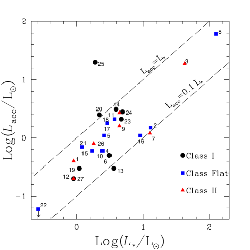
Figure 12: $L_{acc}$ values plotted as a function of $L_{*}$ for the all sample. The two dashed lines show the loci of $L_{acc}=L_{*}$ and $L_{acc}=0.1L_{*}$. The different symbols indicate the class of the objects: Class I, Flat, or Class II (dots, squares, and triangles, respectively). The object IDs are also reported.

5.1.2 Mass accretion rates and accretion evolution

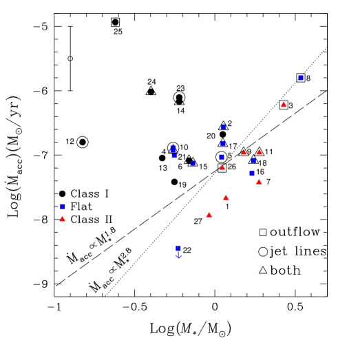
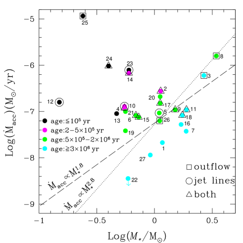
Figure 13: Top panel: Mass accretion rate versus stellar mass for the all sample. The different symbols indicate the class of the objects: Class I, Flat, or Class II (dots, squares, and triangles, respectively). The object ID is also reported. The presence of jets/outflows in the images, lines tracing jets in the spectra, or both are indicated by open squares, circles, or triangles, respectively. The dashed line shows the $\dot{M}_{acc}\propto M_{*}^{1.8}$ relationship obtained by Natta et al. (2006) for the Ophiuchus sample, whereas the dotted line displays the $\dot{M}_{acc}\propto M_{*}^{2.8}$ relationship obtained by Fang et al. (2009) for the L 1634 and the L 1641 samples. The lines are merely indicative and do not fit the data. Bottom panel: Same as top panel, with colours indicating the different age of the objects, ranging from $\leq$10⁵ to 10⁷ yr.

The top panel of Figure 13 shows the mass accretion rates of the sampled objects versus their stellar masses. Again, the various symbols indicate the different classification of the objects (Class I, Flat, and Class II are represented as dots, squares, and triangles, respectively), as also reported in Fig. 12. The presence of jets/outflows in the images, lines tracing jets in the spectra, or both is indicated by open squares, circles, or triangles, respectively, over-plotted on each object.

Several authors have pointed out the existence of an empirical relationship between the mass accretion rate and the stellar mass, i. e. $\dot{M}_{acc}\propto M_{*}^{k}$, with $k$ ranging from $\sim$2 (Calvet et al., 2004; Muzerolle et al., 2003; Natta et al., 2004, 2006) to $\sim$3 (Fang et al., 2009). Our data marginally indicate such a trend, because of the large spread in $\dot{M}_{acc}$ (more than 3 orders of magnitude) and YSO age, the small $M_{*}$ range, and the small number of objects, thus our data do not allow us to obtain a better estimate for $k$. In the figure we also show the $\dot{M}_{acc}\propto M_{*}^{1.8}$ relationship derived by Natta et al. (2006) (dashed line) for their Ophiuchus sample, and the $\dot{M}_{acc}\propto M_{*}^{2.8}$ relationship from Fang et al. (2009) (dotted line) for their L 1634 and L 1641 samples. The lines serve as a guide to the eye and are not intended to fit the data.

As mentioned in Sect. 4.4.6, the outbursting source # 25 shows the highest mass accretion rate, and, in general, when considering a power-law relationship, Class I objects have mass accretion rates higher than the other YSOs, being positioned mostly in the top-left area of the panel. The remaining Class I YSOs are located in the central part of the plot, together with the majority of Flat YSOs. Finally, moving towards the bottom-right part of the panel, there are Class II and a few Flat YSOs. The bottom end is occupied by YSOs, that do not show any evidence of outflow activity. In conclusion, there is a marginal trend between the mass accretion rate evolution and the YSO class. Indeed, this is related to the fact that YSO class is not strictly related to YSO age, as already shown in Sect. 4.4.5 and Fig. 11

On the other hand, there is a more clear correlation between the mass accretion evolution and the age of the YSOs, as shown in the bottom panel of Figure 13, which displays the same $\dot{M}_{acc}$ vs $M_{*}$ plot, with different colours indicating different age ranges. In this case a clear age stratification is visible in the figure, going from the top-left (youngest sources) to the bottom-right (oldest sources) of the panel. Moreover, if we consider objects in the same age range (i. e. YSOs with the same colour in the plot), we note some spread, with high accretors (i. e. with large $L_{acc}/L_{bol}$ ratio) usually positioned at the top-left of their group, and low accretors at the bottom-right. For example the black points (age$\lesssim$10⁵ yr) have source # 25 with $L_{acc}/L_{bol}\sim 0.9$ at one end, and source # 13 with $L_{acc}/L_{bol}\sim 0.1$ at the other. Notably, this low-accreting Class I source does not show any relevant ejection activity in our images and spectra. The violet subsample (age $\sim$2–5$\times$10⁵ yr) has source # 14 with $L_{acc}/L_{bol}\sim 0.4$ and source # 2 with $L_{acc}/L_{bol}\sim 0.1$, and so on. This spread is usually less than one order of magnitude for the various considered age-bins, except for the black points with the outbursting source # 25 ($\sim$ 2 orders of magnitude). Although the largest spread is due to the outburst, the small spreads ($\leq 1$ dex) might be attributed to several causes: i) uncertainties on both $\dot{M}_{acc}$ and $M_{*}$ values; ii) uncertainties on the stellar age; iii) short-time scale variability; iv) differences in the initial and environmental conditions (see, Natta et al., 2006, for a detailed discussion). As stated in Sect. 4.4.6, $\dot{M}_{acc}$ errors can be up to one dex and might cause the spread. There are large uncertainties on the determination of the stellar age, due to our uncertainties on $L_{*}$ and $T_{eff}$. On the other hand, Tab. 2 indicates that, with the exception of the outbursting source # 25, short-time scale variability cannot be responsible for such a large spread. Indeed, the maximum $\sim$10 yr variability in the $K_{s}$ band is $\lesssim$0.5 mag, and, on average, $<$0.2 mag. This type of variability is extremely common in YSOs (see, e. g., Beck, 2007). Even assuming that extinction has not changed and the observed variability in the $K_{s}$ band is entirely due to Br$\gamma$ variation (i. e. to accretion), this translates into a Br$\gamma$ flux change of $\sim$1.6, i. e. less than a factor of 4 in $\dot{M}_{acc}$, that is well below the desired one dex.

Despite the large uncertainties on $\dot{M}_{acc}$, $M_{*}$, and age, Figure 13 (bottom panel) indicates that the large scatter can be, at least partially, explained in terms of YSO age and long-time scale variability. Mass accretion evolution has been studied for T Tauri discs (Hartmann et al., 1998), and mass accretion rates are thought to decrease with time as $\dot{M}_{acc}\propto t^{-\eta}$, consistently with the evolution of a viscous disc (Hartmann et al., 1998; Muzerolle et al., 2000; Sicilia-Aguilar et al., 2006, 2010). According to these viscous disc models, the main infall process from envelope to disc is over, thus the envelope is not providing a significant amount of mass and angular momentum to the disc. Additionally, from this stage on, the quantity of angular momentum removed by the jet/wind is considered irrelevant. Therefore, the disc evolution is mostly driven by viscous processes, which control the mass accretion rate. Once the initial disc mass ($M_{d}$) and viscosity parameter are set, these models predict that the mass accretion decreases exponentially with time. Top panel of Figure 14 shows the accretion rates of the sampled objects as a function of the stellar age, with different colours indicating different mass ranges. Again, the data show a clear trend of the mass accretion decaying with time. This trend matches well the results of other works (Hartmann et al., 1998; Sicilia-Aguilar et al., 2006, 2010), with our data having a smaller $\dot{M}_{acc}$ spread for a given mass interval. For comparison, the black dashed line shows the fiducial model of Hartmann et al. (1998) viscous disc. The model assumes a stellar mass $M_{*}$ of 0.5 $M_{\sun}$, a disc temperature at 100 AU of 10 K, an initial disc mass $M_{d}$ of 0.1 $M_{\sun}$, a viscosity parameter $\alpha$ = 10^-2, and viscosity exponent $\gamma=1$, i. e. $\eta=1.5$ in the $\dot{M}_{acc}\propto t^{-\eta}$ relationship. The curve reproduces well the distribution of our YSOs with $0.4\leq M_{*}\leq 1.2$ $M_{\sun}$ (i. e. violet and red dots). Additionally, more massive and less massive YSOs are positioned above and below the curve, respectively. This is expected, since we observe a correlation between $\dot{M}_{acc}$ and $M_{*}$. The Hartmann et al. (1998) model would probably better match our data using a slightly smaller initial disc mass, which would shift the curve downwards, and a slightly smaller $\eta$ value, which would decrease the curve steepness (-$\eta$ is the curve slope). This last parameter is particularly important, because it regulates the accretion rate, giving us indication of the disc lifetime. To get a better estimate of the $\eta$ parameter, we then fit those data points with age $t>10^{5}$ yr, i. e. in a temporal range where the viscous processes likely control the mass accretion rate. Additionally, we constrain our sample to stellar masses $0.4\leq M_{*}\leq 1.2$ $M_{\sun}$, to be consistent with models and data from the literature. The red dotted line shows the best linear fit to the considered data points (namely violet and red dots with $t>10^{5}$ yr), giving $\eta$ = 1.2$\pm$0.4. An identical result ($\eta\sim 1.2$) was obtained by Sicilia-Aguilar et al. (2010) from their Cep OB2 sample. The authors remark that the mass accretion decay appears to be slower than previously assumed in the models, where $\eta$ values range from 1.5 to 2.8 (Hartmann et al., 1998). To take into account the $\dot{M}_{acc}$ dependence from $M_{*}$ and reduce the scatter in the plot, we normalise $\dot{M}_{acc}$ dividing by $M_{*}^{2}$. The results are shown in the bottom panel of Figure 14. The data scatter is smaller, although the most massive stars are still positioned well above the average. Considering the data points with $t>10^{5}$ yr, we obtain $\eta$=1.0$\pm$0.3, or, discarding the most massive objects ($M_{*}\geq$1.5 $M_{\sun}$, i. e. yellow and green data points), $\eta$=1.3$\pm$0.2.

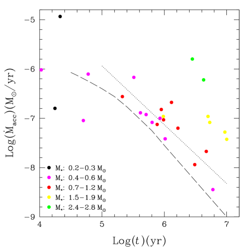
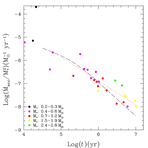
Figure 14: Top panel: Mass accretion rate as a function of stellar age for the observed sample. The various colours indicate different mass values. The dashed line displays one of the viscous models of Hartmann et al. (1998), for a $M_{*}=0.5$ $M_{\sun}$, an initial disc mass $M_{d}=0.1$ $M_{\sun}$, viscosity parameter $\alpha$ = 10^-2, and viscosity exponent $\gamma=1$, i. e. $\eta=1.5$ in the $\dot{M}_{acc}\propto t^{-\eta}$ relationship. The red dotted line shows the best linear fit for data points with $0.4\leq M_{*}\leq 1.2$ $M_{\sun}$ and $t>10^{5}$ yr, i. e. $\dot{M}_{acc}\propto t^{-1.2}$. Bottom panel: Same as top panel, but with the $\dot{M}_{acc}$ values normalised to the stellar $M_{*}^{2}$, to take into account $\dot{M}_{acc}$ dependence from $M_{*}$.

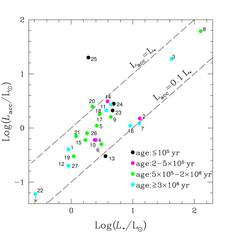
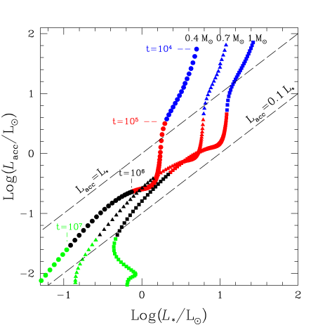
Figure 15: Top panel: $L_{acc}$ vs $L_{*}$ as in Fig. 12, with colours indicating the different age of the objects as bottom panel of Fig. 13. Bottom panel: Simulation of the $L_{acc}$ vs $L_{*}$ temporal evolution for YSOs of different masses (0.4, 0.7, and 1 $M_{\sun}$), derived considering the evolutionary tracks from Siess et al. (2000) and a viscous disc evolution with $\dot{M}_{acc}\propto t^{-\eta}$, with $\eta$=1.2. Different colours indicate different age, ranging from 10⁴ to 10⁷ yr.

Finally, on the basis of our previous results, it is reasonable to question whether the scatter observed in the $L_{acc}$ vs $L_{*}$ plot of Figure 12 might be related to the inferred mass accretion evolution. Naively, we might expect an age stratification in the plot similar to what we observe in the $\dot{M}_{acc}$ vs $M_{*}$, with younger objects showing larger $L_{acc}/L_{*}$ ratios and the older YSOs with smaller ratios. However, if we plot $L_{acc}$ vs $L_{*}$ as a function of the age as in Fig. 13, bottom panel, there is not any stratification (see Fig. 15, top panel). Besides the uncertainties on $L_{*}$ and $L_{acc}$, which indeed affect our results, this is because $L_{acc}$ does not depend only on $\dot{M}_{acc}$, but also on the $M_{*}/R_{*}$ ratio, which is not linear.

To clarify this point, we simulate the temporal evolution of $L_{acc}$ vs $L_{*}$, for YSOs with 0.4, 0.7, and 1 $M_{\sun}$ stellar masses, using Siess et al. (2000) evolutionary tracks, and assuming an $\dot{M}_{acc}$ evolution with $\dot{M}_{acc}\propto t^{-1.2}$. The bottom panel of Figure 15 shows the results of our simulation, with different colours and labels indicating various age bins, from 10⁴ to 10⁷ yr. According to this plot, objects with the same age but with different stellar mass usually have different $L_{acc}/L_{*}$ values, which increase with $M_{*}$. More notably, for a given $M_{*}$, the $L_{acc}/L_{*}$ ratio does not decrease monotonically with time, but, between 10⁵ and 10⁶ yr, the function shows a local minimum (coloured red in the plot), which appears at earlier times with increasing stellar mass (see Figure 15, bottom panel). Indeed, our oversimplified simulation does not take into account other important factors like mass accretion variability, and different environmental and initial conditions, which may strongly affect the $L_{acc}$ value, producing a more confused outcome. Nevertheless, it might explain, at least partially, the $L_{acc}/L_{*}$ spreads so far observed in the literature and here.

5.1.3 Mitigating the luminosity problem?

Several observational studies have already shown that a significant discrepancy exists between the accretion rates observed in embedded YSOs and those predicted by theoretical models. This inconsistency was first noted by Kenyon et al. (1990), and it is also known as the luminosity problem (Kenyon & Hartmann, 1995), because the early-YSO luminosities, which should be accretion dominated, appear to be fainter than expected. The latest Spitzer Space Telescope surveys (see, e. g., Evans et al., 2009; Enoch et al., 2009) support these findings, revealing that more than 50% of the embedded YSOs have bolometric luminosities, and thus inferred mass accretion rates, considerably lower than those predicted by the free-fall theoretical models (i. e. $\dot{M}_{acc}<<$10^-6 $M_{\sun}$ yr^-1 vs $\sim$2$\times$10^-6 $M_{\sun}$ yr^-1, for a Class I YSO with M$\sim$1 $M_{\sun}$; Shu, 1977; Terebey et al., 1984). More evidence comes from recent NIR spectral studies of Class I YSOs (White & Hillenbrand, 2004; Nisini et al., 2005a; Doppmann et al., 2005; Antoniucci et al., 2008; Beck, 2007; Prato et al., 2009), aimed at measuring both stellar and accretion luminosities, and at estimating the stellar age. These studies have shown that, on average, a large fraction of Class I YSOs has mass accretion and ejection rates lower than theoretically expected (from one to two orders of magnitude), i. e. more similar to the accretion rates of the classical T Tauri stars ($\sim$10⁶ yr). To reconcile theory with observations, these studies provide various motivations.

For example, misclassification might be one of the causes, and some Class I objects are likely to be misclassified Class II YSOs, seen through optically thick discs. Indeed, geometrical effects can easily modify the SED shape and thus the observed spectral index (see, e. g., Whitney et al., 2003b). Nevertheless, radiative transfer models of Whitney et al. (2003b) clearly indicate that misclassified objects are about five times fainter than real Class I YSOs, and we actually observe these difference in our sample (see, e. g., source # 19 vs # 23 in Table 7). White et al. (2007) suggest that at least one-third of Class I YSOs in Taurus have been misclassified, and we find the same result in our small sample, i. e. three (namely # 6, # 19, and # 20) out of nine Class I YSOs have ages $\sim$1 Myr, i. e. they are likely edge-on CTT stars.

However, results from this and other works indicate that several Class I YSOs are genuine young stellar objects ($\leq$5$\times$10⁵ yr) with accretion rates ranging from $\sim$$\dot{M}_{acc}\sim$10^-6 to 10^-8 $M_{\sun}$ yr^-1. Therefore, to reach their final masses, these YSOs cannot accrete mass in a steady way, but they need to acquire most of their mass through short episodic outbursts, during which $\dot{M}_{acc}$ increases by some order of magnitudes up to $\dot{M}_{acc}$$\sim$10^-5 $M_{\sun}$ yr^-1 for YSOs with $\sim$1 $M_{\sun}$.

The results of our survey, although biased by the relatively small number of targets and by the sample selection criteria, are consistent with this picture. A small number of very young objects (‘true’ Class I YSOs) shows high mass accretion rates. Among them we detected an outbursting YSO (source # 25), which has recently increased its mass accretion rate by $\sim$2 orders of magnitude (Caratti o Garatti et al., 2011), whereas the remaining sources have, on average, $\dot{M}_{acc}\sim$5$\times$10^-7 $M_{\sun}$ yr^-1 (six objects with $M_{*}\lesssim$1 $M_{\sun}$) and $\dot{M}_{acc}\sim$10^-7 $M_{\sun}$ yr^-1 (one object with $M_{*}\sim$0.1 $M_{\sun}$). Considering different ranges of masses, these $\dot{M}_{acc}$ values are almost one order of magnitude higher than those reported by White et al. (2007), implying that these young objects should spend $\sim$5% of their time in an outburst state to reach typical CTT masses, i. .e. this percentage is slightly smaller than White et al. (2007) estimates. Therefore, statistically, we should observe that among ‘true’ Class I sources about $\sim$5% of these objects are in a outburst phase, while the remaining are quiescent, and thus ‘under-luminous’. So far our statistics is pretty limited and a larger number of deep-NIR imaging surveys is needed. Nevertheless, the results of the latest NIR surveys, which discovered several embedded outbursting YSOs (see, e. g., Covey et al., 2011; Kóspál et al., 2011; Caratti o Garatti et al., 2011), seem to point in this direction.

6 Conclusions

As part of the POISSON project (Protostellar Optical-Infrared Spectral Survey On NTT), we present the results of a multi-wavelength spectroscopic and photometric survey of 27 embedded YSOs in the L 1641 star forming region, aimed at deriving the stellar parameters and evolutionary stage, as well as inferring their accretion and ejection properties. Our multi-wavelength database includes low-resolution optical-IR spectra from NTT and Spitzer (0.6-40 $\mu$m), as well as photometric data covering a spectral range from 0.4 to 1100 $\mu$m, which allow us to construct the YSOs spectral energy distributions (SEDs) and to characterise the object parameters (visual extinctions, spectral types, accretion and bolometric luminosities, mass accretion and ejection rates).

The main observational results of this work are the following:

1. Photometric variability of $\Delta m_{K}\geq$0.3 mag is detected in $\sim$22% of the YSOs ($\sim$10 yr baseline).

2. The optical-NIR spectra show several emission lines, mostly associated with YSO accretion and ejection activity (e. g., H i, Ca ii, He i, [S ii], [Fe ii], H₂), as well as other emission lines (e. g. O i, Fe i Na i, Mg ii, C i) characteristic of active young stars, broad-band molecular absorption features, typical of cool objects (VO, TiO and H₂O bands) and CO overtone bands both in absorption and emission. Also Spitzer spectra show emission lines, mostly H₂ pure rotational lines, [Fe ii], [Si ii] and [Si iii], and [S iii], largely originating from shocks along the YSOs jets, or tracing the disc. Ice absorption features at 5 to 8 $\mu$m (H₂O) and 15.2 $\mu$m (CO₂), as well as the amorphous silicate absorption feature at 9.7 $\mu$m have been also detected in some of the sources.

3. SEDs were constructed using both photometric and spectroscopic data, allowing to classify the 27 targets as nine Class I, eleven Flat, and seven Class II YSOs. The inferred $L_{bol}$ values range from $\sim$0.3 to 180 $L_{\sun}$.

4. The spectral types for the sample range from B7 to M7.5, with 74% of the objects being low-mass YSOs (SpT$\geq$K5). The average and median age of the sample are about 2 and 1 Myr, respectively, with values ranging from $\leq$10⁵ to 10⁷ yr. The average ages of Class I YSOs, Flat, and Class II YSOs are 0.4, 2, and 4 Myr. Six out of nine Class I YSOs have an age of $\sim$10⁵, while the remaining three appear to be older (5$\times$10⁵ to 10⁶ yr). Also among the Flat sources there are three objects (out of eleven) with age $\geq$5$\times$10⁶ yr, i. e. consistent with more evolved sources.

5. Accretion luminosities, obtained by averaging luminosities from Pa$\beta$, and Br$\gamma$ lines, range from $\sim$0.1 to $\sim$60 $L_{\sun}$, whereas mass accretion rates range from 3.6$\times$10^-9 to 1.2$\times$10^-5 M_☉ yr^-1.

From these results we draw the following conclusions:

1. Geometrical effects can significantly modify the SED shapes, and the standard SED classification ($\alpha$ computed between 2.2 and 24 $\mu$m) may not properly reflect YSO age.

2. Mass accretion and ejection rates, extinction, and spectral indices decrease with YSO age. The youngest YSOs have the highest mass accretion rates, whereas the oldest YSOs do not show detectable jet activity in both images and spectra. Nevertheless, apart from the outbursting source # 25 and, marginally, source # 20, none of the remaining YSOs is accretion dominated (i. e. having $L_{acc}>L_{*}$).

3. There is a marginal trend between the mass accretion rate evolution and the YSO class, whereas there is a more clear correlation between the mass accretion evolution and the age of the YSOs. Despite the large uncertainties on $\dot{M}_{acc}$, $M_{*}$, and age, our analysis indicates that the large spread of mass accretion rates can be mostly explained in terms of YSO age and long-time scale (non-periodic) variability.

4. We obtain a clear correlation between $\dot{M}_{acc}$ and age ($\dot{M}_{acc}\propto t^{-\eta}$, with $\eta$=1.2), for YSOs with $t>10^{5}$ yr, consistent with the mass accretion evolution in viscous disc models. These results indicate that the mass accretion decay appears to be slower than previously assumed in the classical models (Hartmann et al., 1998) (where the $\eta$ value ranges from 1.5 to 2.8) and coincides with the latest results.

5. The majority of very young objects in our sample (‘true’ Class I YSOs, $t\leq$5$\times$10⁵ yr) shows, on average, high mass accretion rates. Among them, we detected an outbursting YSO (source # 25), which has recently increased its mass accretion rate by $\sim$2 orders of magnitude, whereas the remaining sources have, on average, $\dot{M}_{acc}\sim$5$\times$10^-7 $M_{\sun}$ yr^-1 (six objects with $M_{*}\lesssim$1 $M_{\sun}$) or $\dot{M}_{acc}\sim$10^-7 $M_{\sun}$ yr^-1 when considering less massive objects ($M_{*}\sim$0.1 $M_{\sun}$). Considering different ranges of masses, these $\dot{M}_{acc}$ values are almost one order of magnitude higher than those previously studied, e. g. in Taurus and Auriga star forming regions, implying that these young objects should spend 1–5% of their lifetime in an outburst state, to reach typical CTTs masses.

Appendix A Photometry & Spectroscopy

Table 9: Available photometry from 0.44 $\mu$m to 8 $\mu$m (Jy)

Source	B	V	R	IB	IJ	J	H	Ks	IRAC 1	IRAC 2	IRAC 3	IRAC 4
ID	0.44 $\mu$m	0.55 $\mu$m	0.64 $\mu$m	0.79 $\mu$m	0.9 $\mu$m	1.25 $\mu$m	1.65 $\mu$m	2.2 $\mu$m	3.6 $\mu$m	4.5 $\mu$m	5.8 $\mu$m	8.0 $\mu$m
1	$\cdots$	$\cdots$	0.003$\pm$0.001	0.004$\pm$0.001	0.021$\pm$0.005	0.0224$\pm$0.0009	0.066$\pm$0.002	0.089$\pm$0.002	0.122$\pm$0.007	0.115$\pm$0.006	0.103$\pm$0.006	0.097$\pm$0.005
2	6e-5$\pm$2e-5	$\cdots$	0.001$\pm$0.0003	0.005$\pm$0.001	0.0055$\pm$0.0005	0.048$\pm$0.001	0.166$\pm$0.005	0.347$\pm$0.007	0.651$\pm$0.006	0.83$\pm$0.001	0.97$\pm$0.01	1.17$\pm$0.01
3	0.12$\pm$0.03	0.23$\pm$0.05	$\cdots$	0.43$\pm$0.06	0.25$\pm$0.03	0.91$\pm$0.02	1.68$\pm$0.04	2.79$\pm$0.06	2.09$\pm$0.09	$\cdots$	4.1$\pm$0.1	5.0$\pm$0.1
4	0.0016$\pm$0.0003	0.0043$\pm$0.0008	0.007$\pm$0.0019	0.018$\pm$0.003	0.018$\pm$0.003	0.059$\pm$0.002	0.089$\pm$0.003	0.104$\pm$0.003	0.116$\pm$0.002	0.137$\pm$0.004	0.156$\pm$0.004	0.221$\pm$0.006
5	$\cdots$	$\cdots$	4e-5$\pm$1e-5	23e-5$\pm$6e-5	0.0004$\pm$0.0002	0.0092$\pm$0.0003	0.03911$\pm$0.0009	0.076$\pm$0.002	0.147$\pm$0.003	0.203$\pm$0.004	0.245$\pm$0.007	0.382$\pm$0.007
6	$\cdots$	$\cdots$	$\cdots$	$<$9e-5	2e-5$\pm$1e-5	0.0010$\pm$0.0005	0.004$\pm$0.002	0.0128$\pm$0.0008	0.097$\pm$0.004	0.184$\pm$0.003	0.240$\pm$0.007	0.266$\pm$0.005
7	0.003$\pm$0.002	$\cdots$	0.028$\pm$0.001	0.045$\pm$0.002	0.19$\pm$0.005	0.169$\pm$0.003	0.265$\pm$0.007	0.43$\pm$0.01	0.73$\pm$0.04	0.86$\pm$0.05	0.88$\pm$0.05	1.70$\pm$0.09
8	3e-5$\pm$1e-5	$\cdots$	0.0006$\pm$0.0002	$\cdots$	0.00024$\pm$0.00007	0.317$\pm$0.007	2.02$\pm$0.06	5.8$\pm$0.1	$\cdots$	$\cdots$	15.7$\pm$0.1	$\cdots$
9	$\cdots$	$\cdots$	0.010$\pm$0.001	0.022$\pm$0.002	0.032$\pm$0.005	0.128$\pm$0.003	0.289$\pm$0.007	0.41$\pm$0.01	0.372$\pm$0.007	0.324$\pm$0.006	0.274$\pm$0.007	0.323$\pm$0.006
10	$\cdots$	$\cdots$	0.00023$\pm$0.00004	0.00095$\pm$0.00005	0.0008$\pm$0.0003	0.0123$\pm$0.0003	0.0290$\pm$0.0006	0.040$\pm$0.001	0.084$\pm$0.005	0.108$\pm$0.008	0.14$\pm$0.01	0.19$\pm$0.01
11	$\cdots$	$\cdots$	0.005$\pm$0.002	0.013$\pm$0.002	0.050$\pm$0.003	0.105$\pm$0.002	0.220$\pm$0.003	0.36$\pm$0.01	0.44$\pm$0.03	0.49$\pm$0.03	0.55$\pm$0.03	0.52$\pm$0.03
12	$\cdots$	$\cdots$	35e-5$\pm$5e-5	0.0010$\pm$0.0002	0.0004$\pm$0.0002	0.0123$\pm$0.0006	0.0220$\pm$0.0006	0.0242$\pm$0.0006	0.021$\pm$0.001	0.0236$\pm$0.001	0.032$\pm$0.002	0.050$\pm$0.003
13	$\cdots$	$\cdots$	$\cdots$	$\cdots$	$\cdots$	0.00029$\pm$0.0001	0.0007$\pm$0.0002	0.0027$\pm$0.0009	0.054$\pm$0.005	0.081$\pm$ 0.006	0.075$\pm$0.006	0.090$\pm$0.007
14	$\cdots$	$\cdots$	$\cdots$	$\cdots$	$\cdots$	0.0010$\pm$0.0001	0.0089$\pm$0.0002	0.042$\pm$0.001	0.241$\pm$0.004	0.413$\pm$0.004	0.576$\pm$0.009	0.793$\pm$0.009
15	9e-5$\pm$2e-5	$\cdots$	0.0009$\pm$0.0002	0.0018$\pm$0.0005	0.0031$\pm$0.0005	0.0093$\pm$0.0002	0.0285$\pm$0.0007	0.055$\pm$0.001	0.099$\pm$0.003	0.116$\pm$0.003	0.127$\pm$0.005	0.177$\pm$0.003
16	0.0013$\pm$0.0003	$\cdots$	0.0156$\pm$0.004	0.04$\pm$0.01	0.045$\pm$0.005	0.202$\pm$0.004	0.329$\pm$0.008	0.45$\pm$0.02	0.507$\pm$0.005	0.490$\pm$0.009	0.453$\pm$0.008	0.774$\pm$0.007
17	$\cdots$	$\cdots$	$\cdots$	$\cdots$	$\cdots$	37e-5$\pm$4e-5	0.0084$\pm$0.0002	0.0410$\pm$0.0009	0.102$\pm$0.002	0.163$\pm$0.004	0.230$\pm$0.006	0.325$\pm$0.006
18	0.012$\pm$0.004	0.022$\pm$0.008	$\cdots$	$\cdots$	0.07$\pm$0.01	0.091$\pm$0.002	0.120$\pm$0.003	0.129$\pm$0.003	0.19$\pm$0.01	0.26$\pm$0.01	0.34$\pm$0.02	0.52$\pm$0.03
19	$\cdots$	$\cdots$	$\cdots$	$\cdots$	2e-5$\pm$1e-5	5e-5$\pm$1e-5	0.0004$\pm$2e-5	0.0076$\pm$0.0002	0.036$\pm$0.001	0.049$\pm$0.001	0.060$\pm$0.003	0.080$\pm$0.003
20	$\cdots$	$\cdots$	$\cdots$	$\cdots$	$\cdots$	0.0003$\pm$0.0001	0.0060$\pm$0.0002	0.0399$\pm$0.0007	0.218$\pm$0.004	0.314$\pm$0.006	0.419$\pm$0.008	0.474$\pm$0.008
21	$\cdots$	$\cdots$	$\cdots$	$\cdots$	$\cdots$	$<$0.0003	0.0013$\pm$0.0001	0.0121$\pm$0.0003	0.043$\pm$ 0.002	0.069$\pm$0.001	0.087$\pm$0.003	0.099$\pm$0.003
22	$\cdots$	$\cdots$	$\cdots$	$\cdots$	2e-5$\pm$1e-5	0.0013$\pm$6e-5	0.0079$\pm$0.0002	0.0158$\pm$0.0004	0.0106$\pm$0.001	0.020$\pm$0.002	0.022$\pm$0.002	0.025$\pm$0.006
23	$\cdots$	$\cdots$	$\cdots$	$\cdots$	2e-5$\pm$1e-5	0.0008$\pm$6e-5	0.0087$\pm$0.0002	0.0386$\pm$0.0004	0.136$\pm$0.003	0.253$\pm$0.005	0.352$\pm$0.007	0.45$\pm$0.01
24	$\cdots$	$\cdots$	$\cdots$	$\cdots$	3e-5$\pm$1e-5	86e-5$\pm$6e-5	0.0056$\pm$0.0002	0.0250$\pm$0.0006	0.090$\pm$0.002	0.167$\pm$0.003	0.302$\pm$0.008	0.386$\pm$0.007
25	$\cdots$	$\cdots$	$\cdots$	$\cdots$	1e-5$\pm$1e-5	0.00044$\pm$4e-5	0.0040$\pm$0.0001	0.0132$\pm$0.0004	0.121$\pm$0.007	0.18$\pm$0.01	0.20$\pm$0.01	0.23$\pm$0.01
26	$\cdots$	$\cdots$	$\cdots$	9e-5$\pm$1e-5	0.0002$\pm$1e-5	0.0107$\pm$0.0002	0.061$\pm$0.001	0.154$\pm$0.003	0.22$\pm$0.01	0.29$\pm$0.02	0.32$\pm$0.02	0.32$\pm$0.02
27	5e-5$\pm$1e-5	$\cdots$	30e-5$\pm$7e-5	0.0011$\pm$0.0003	0.0019$\pm$0.0009	0.0120$\pm$0.0002	0.0324$\pm$0.0006	0.0479$\pm$0.0009	0.042$\pm$0.002	0.045$\pm$0.002	0.030$\pm$0.002	0.024$\pm$0.002

Table 10: Available photometry from 24 $\mu$m to 1100 $\mu$m (Jy)

Source	MIPS 1	MIPS 2	MIPS 3	UKT14	SCUBA	UKT14	SCUBA	UKT14
ID	24 $\mu$m	70 $\mu$m	160 $\mu$m	350 $\mu$m	450 $\mu$m	800 $\mu$m	850 $\mu$m	1100 $\mu$m
1	0.172$\pm$0.005	$\cdots$	$\cdots$	$\cdots$	$\cdots$	$\cdots$	$\cdots$	$\cdots$
2	4.5$\pm$0.3	11.2$\pm$0.5	$\cdots$	6.52$\pm$2.1	3.75$\pm$0.27	0.635$\pm$0.032	$\cdots$	0.239$\pm$0.039
3	6.6$\pm$0.8	6.5$\pm$2.2	$\cdots$	$\cdots$	2.540$\pm$0.06	0.9$\pm$0.06	$\cdots$
4	0.88$\pm$0.08	1.5$\pm$0.2	$\cdots$	$\cdots$	$\cdots$	$\cdots$	$\cdots$	$\cdots$
5	0.97$\pm$0.04	1.4$\pm$0.1	2.5$\pm$1	$\cdots$	$\cdots$	$\cdots$	$\cdots$	$\cdots$
6	1.2$\pm$0.1	5.2$\pm$0.6	4$\pm$1	$\cdots$	1.42$\pm$0.13	0.19$\pm$0.014	$\cdots$	$\cdots$
7	2.6$\pm$0.1	4.1$\pm$0.2	6$\pm$1	$\cdots$	$\cdots$	$\cdots$	$\cdots$	$\cdots$
8	52$\pm$2	97$\pm$1	35$\pm$9	13.7$\pm$0.29	9.04$\pm$0.06	1.90$\pm$0.087	1.40$\pm$0.06	0.767$\pm$0.06
9	0.74$\pm$0.02	0.8$\pm$0.1	$\cdots$	$\cdots$	$\cdots$	$\cdots$	$\cdots$	$\cdots$
10	0.48$\pm$0.05	0.6$\pm$0.1	$\cdots$	$\cdots$	$\cdots$	$\cdots$	$\cdots$	$\cdots$
11	1.32$\pm$0.07	4.0$\pm$0.7	$<$6	$\cdots$	$\cdots$	$\cdots$	$\cdots$	$\cdots$
12	0.45$\pm$0.03	0.8$\pm$0.2	$\cdots$	$\cdots$	$\cdots$	$\cdots$	$\cdots$	$\cdots$
13	1.7$\pm$0.1	5.4$\pm$0.9	5.3$\pm$2.2	$\cdots$	$\cdots$	$\cdots$	$\cdots$	$\cdots$
14	2.3$\pm$0.2	5.4$\pm$0.2	5$\pm$1	$\cdots$	$\cdots$	$\cdots$	$\cdots$	$\cdots$
15	0.51$\pm$0.02	1.6$\pm$0.2	$<$4	$\cdots$	$\cdots$	$<$0.2	$\cdots$	$\cdots$
16	3.2$\pm$0.2	1.6$\pm$0.2	$<$0.8	$\cdots$	$\cdots$	$<$0.2	$\cdots$	$\cdots$
17	0.74$\pm$0.05	1.3$\pm$0.1	3.5$\pm$1	$\cdots$	$\cdots$	0.450$\pm$0.022	$\cdots$	$\cdots$
18	1.91$\pm$0.07	2.3$\pm$0.3	$\cdots$	$\cdots$	$\cdots$	$\cdots$	$\cdots$	$\cdots$
19	0.31$\pm$0.05	1.9$\pm$0.5	$\cdots$	$\cdots$	$\cdots$	$\cdots$	$\cdots$	$\cdots$
20	1.4$\pm$0.1	4.9$\pm$0.5	3$\pm$1	$\cdots$	$\cdots$	0.148$\pm$0.06	$\cdots$	$\cdots$
21	0.26$\pm$0.01	4.4$\pm$0.4	$\cdots$	$\cdots$	$\cdots$	$\cdots$	$\cdots$	$\cdots$
22	0.1$\pm$0.02	$\cdots$	$\cdots$	$\cdots$	$\cdots$	$\cdots$	$\cdots$	$\cdots$
23	4.5$\pm$0.2	10.7$\pm$1.2	3.5$\pm$1.3	$\cdots$	2.3$\pm$0.5	0.7$\pm$0.3	$\cdots$	$\cdots$
24	2.9$\pm$0.2	10.7$\pm$0.6	5.5$\pm$1.4	$\cdots$	2.79$\pm$0.64	$\cdots$	0.7$\pm$0.011	0.289$\pm$0.030
25	0.73$\pm$0.08	1.4$\pm$0.2	0.5$\pm$0.1	$\cdots$	0.2$\pm$0.1	$\cdots$	$\cdots$	$\cdots$
26	0.26$\pm$0.01	0.5$\pm$0.2	$\cdots$	$\cdots$	$\cdots$	$\cdots$	$\cdots$	$\cdots$
27	0.148$\pm$0.008	0.96$\pm$0.22	$\cdots$	$\cdots$	$\cdots$	$\cdots$	$\cdots$	$\cdots$

Table 11: Observed emission lines in [CSH2001]13811 - ID 1.

Line id.	$\lambda$	F	$\Delta$F	FWHM	Wλ
	($\mu$m)	(erg cm-2 s-1)		Å	Å
EFOSC & SofI - NTT
H$\alpha$	0.656	9.53e-14	1.00e-14	11.0	-11.01
Pa $\delta$	1.005	8e-15	3e-15	16.8	-2.0
C i	1.069	7.42e-15	2.00e-15	18.0	-18.0
Pa $\gamma$	1.094	1.09e-14	0.30e-14	19.1	-2.8
Pa $\beta$	1.282	1.8e-14	0.30e-14	21.6	-4.0
Br $\gamma$	2.166	2.96e-14	0.50e-14	55.0	-5.1
Line id.	$\lambda$	F	$\Delta$F	FWHM	Wλ
	($\mu$m)	(Jy $\mu$m)		($\mu$m)	($\mu$m)
IRS - Spitzer
H2	17.0	0.010	0.002	0.25	-0.07
[Fe ii]	22.9	0.014	0.003	0.24	-0.08
[Fe ii]	24.5	0.007	0.003	0.30	-0.04
[Si iii]	25.6	0.028	0.005	0.40	-0.16
H2	28.2	0.031	0.005	0.40	-0.16
[S iii]	33.5	0.053	0.008	0.6	-0.27
[Fe ii]	35.8	0.023	0.007	0.24	-0.09
[Fe i]	36.5	0.068	0.008	0.36	-0.27

Table 11: continued.

Table 12: Observed emission lines in [CTF93] 50 - ID 2.

Line id.	$\lambda$	F	$\Delta$F	FWHM	Wλ
	($\mu$m)	(erg cm-2 s-1)		Å	Å
EFOSC & SofI - NTT
[O i] 1D${}_{2}-^{3}$P2	0.630	7.66e-15	0.16e-15	8.322	-7.065
Fe ii	0.635	0.96e-15	0.30e-15	11.8	-0.87
[O i] 1D${}_{2}-^{3}$P1	0.636	2.66e-15	0.30e-15	9.8	-2.343
Fe ii	0.646	0.78e-15	0.30e-15	8.90	-0.564
Fe i	0.649	1.06e-15	0.40e-15	12.80	-0.857
Fe ii	0.651	1.10e-15	0.40e-15	11.00	-0.6
[N i] 1D${}_{2}-^{3}$P0	0.653	4.43e-14	0.50e-14	11.8	-1.246
H$\alpha$	0.656	9.87e-15	0.40e-15	6.76	-6.96
H$\alpha$ PCygni	0.655	-1.6e-15		4.5	1.1
[S ii] 2D${}_{5/2}-^{4}$S3/2	0.672	3.30e-15	0.30e-15	12.08	-2.14
[S ii] 2D${}_{3/2}-^{4}$S3/2	0.673	5.49e-15	0.25e-15	9.71	-3.4
He i  3Po${}_{2}-0-^{3}$S1	0.706	8.36e-15	0.30e-14	36.2	-4.845
Fe ii	0.707	1.01e-14	0.50e-14	12.2	-0.296
?	0.710	1.00e-14	0.30e-15	35.13	-6.16
?	0.713	1.27e-13	1.00e-14	12.4	-4.45
?	0.715	0.93e-14	0.30e-15	23.64	-5.12
?	0.733	1.60e-15	0.4e-15	14.9	-0.87
?	0.737	2.70e-15	0.4e-15	14.8	-1.424
Pa 20	0.839	2.22e-15	0.10e-14	15.1	-0.77
Pa 19	0.842	2.48e-14	1.00e-14	11.1	-2.619
Pa 18 +	0.844
O i 3P${}_{0}-^{3}$S${}_{1}^{*}$	0.845	5.55e-15	0.10e-14	11.3	-2.07
O i 3P${}_{2}-^{3}$S${}_{1}^{*}$
O i 3P${}_{1}-^{3}$S${}_{1}^{*}$
Pa 16 +	0.850
Ca ii 2P${}_{3/2}-^{2}$D3/2	0.850	1.86e-14	0.20e-14	9.9	-6.66
Ca ii 2P${}_{3/2}-^{2}$D5/2 +	0.854	1.82e-14	0.20e-14	9.9	-6.42
Pa 15	0.855
Pa 14	0.860	2.86e-15	0.10e-14	12.40	-1.0
	0.860	2.00e-15	0.10e-14	9.90	-0.70
N i	0.863	3.88e-15	0.20e-14	20.90	-1.34
Ca ii 2P${}_{1/2}-^{2}$D3/2	0.866	1.65e-14	0.20e-14	10.15	-5.70
Pa 13	0.867	4.43e-15	0.20e-14	16.41	-1.52
Pa 12	0.875	4.92e-15	0.20e-14	17.9	-1.70
Mg i	0.881	4.07e-15	0.20e-14	18.6	-1.43
Pa $\delta$	1.005	2.92e-13	0.10e-13	21.78	-13.1
C i (1)	1.069	1.71e-14	0.40e-14	20.2	-2.92
He iPCygni	1.083	-2.8e-14		15.8	4.64
Si ior Fe ii	1.087	5.31e-14	1.00e-14	20.4	-2.418
Pa $\gamma$	1.094	2.02e-14	0.40e-14	24.3	3.271
C i (24)	1.175	1.23e-14	0.80e-14	19.3	1.53
[P ii] 3P2-1D2 or C i	1.189	2.11e-14	0.80e-14	18.0	2.56
Si i?	1.205	2.46e-14	0.80e-14	21.1	-2.86
[Fe ii] a4D7/2-a6D${}_{9/2}^{*}$	1.257	1.76e-14	0.70e-14	26.9	-1.76
He i?	1.270	3.61e-14	0.80e-14	16.5	-3.59
Pa $\beta$	1.282	4.5e-14	0.40e-14	18.04	-4.4
[Fe ii] a4D7/2-a4F9/2	1.644	2.11e-14	0.80e-14	44.0	-1.156
Br $\gamma$	2.166	7.41e-14	0.80e-14	45.62	-3.33
Line id.	$\lambda$	F	$\Delta$F	FWHM	Wλ
	($\mu$m)	(Jy $\mu$m)		($\mu$m)	($\mu$m)
IRS - Spitzer
[S iii]	33.5	0.18	0.06	0.4	-0.24
[Si ii]	35.3	0.13	0.06	0.2	-0.17
[Fe ii]	35.8	0.19	0.07	0.3	-0.24
[Fe i]	36.5	0.22	0.07	0.3	-0.26

Table 12: continued.

Table 13: Observed emission lines in [CTF93] 47 - ID 3.

Line id.	$\lambda$	F	$\Delta$F	FWHM	Wλ
	($\mu$m)	(erg cm-2 s-1)		Å	Å
EFOSC & SofI - NTT
Fe ii	0.615	3.17e-13	0.10e-13	9.77	-1.755
Fe ii	0.625	6.69e-13	0.10e-13	14.4	-3.68
Fe ii	0.635	3.13e-13	0.10e-13	13.10	-1.781
Fe ii	0.637	3.17e-13	0.10e-13	13.00	-1.754
Fe ii	0.642	2.32e-13	0.10e-13	11.10	-1.27
Fe i	0.643	3.04e-13	0.10e-13	11.80	-1.67
Fe ii	0.646	6.78e-13	0.10e-13	10.00	-3.725
Fe i	0.649	1.81e-13	0.10e-13	16.6	-1.585
Fe i	0.651	4.56e-13	0.10e-13	10.58	-2.502
H$\alpha$	0.656	1.33e-11	1.00e-14	9.68	-73.17
He i 3Po${}_{2}-0-^{3}$S1	0.667	9.35e-14	1.00e-14	11.48	-0.508
Fe i?	0.697	1.26e-13	2.00e-14	16.3	-0.68
Fe ii	0.746	2.89e-13	3.00e-14	12.8	-1.76
Fe ii	0.751	1.98e-13	3.00e-14	12.4	-1.22
Fe ii	0.771	3.64e-13	4.00e-14	12.0	-2.42
O i 5P${}_{0}-^{5}$S${}_{1}^{*}$	0.777	5.36e-13	4.00e-14	10.79	-3.567
Mg ii	0.787	2.22e-13	5.00e-14	17.7	-1.54
Mg ii	0.789	2.72e-13	5.00e-14	12.6	-1.91
Si i	0.794	1.78e-13	5.00e-14	10.6	-1.285
Pa 22	0.836	1.53e-13	5.00e-14	14.1	-1.198
Pa 19	0.842	1.30e-13	5.00e-14	10.6	-1.0
Pa 18 +	0.844
O i 3P${}_{0}-^{3}$S${}_{1}^{*}$	0.845	8.22e-13	5.00e-14	11.00	-6.37
O i 3P${}_{2}-^{3}$S${}_{1}^{*}$
O i 3P${}_{1}-^{3}$S${}_{1}^{*}$
Pa 17	0.847	1.89e-13	5.00e-14	10.0	-1.46
Pa 16 +	0.850
Ca ii 2P${}_{3/2}-^{2}$D3/2	0.850	3.13e-12	5.00e-14	10.0	-24.2
Ca ii 2P${}_{3/2}-^{2}$D5/2 +	0.854	3.44e-12	5.00e-14	10.3	-26.6
Pa 15	0.855
Pa 14	0.860	2.80e-13	0.40e-13	12.0	-2.15
Ca ii 2P${}_{1/2}-^{2}$D3/2 +	0.866	3.04e-12	5.00e-14	10.32	-23.67
Pa 13	0.867
Pa 12	0.875	3.39e-13	5.00e-14	12.7	-2.77
Mg i	0.881	3.57e-13	5.00e-14	14.7	-3.13
Fe i	0.882	2.20e-13	5.00e-14	16.7	-1.95
Pa 11	0.887	3.63e-13	5.00e-14	10.0	-3.24
Ca ii 2F${}^{0}_{5/2}-^{2}$D3/2	0.891	2.55e-13	5.00e-14	13.0	-2.3
Pa 10	0.902	4.02e-13	1.00e-13	12.9	-4.7
Pa 9	0.923	8.79e-13	1.00e-13	26.0	-10.42
Pa 8	0.955	1.06e-12	0.80e-13	17.91	-5.67
Fe ii	1.000	1.25e-12	0.80e-13	17.0	-5.35
Pa $\delta$	1.005	1.52e-12	0.80e-13	16.00	-8.24
Fe ii	1.051	7.83e-13	0.80e-13	20.8	-5.35
C i (1)	1.069	5.91e-13	0.80e-13	20.50	-3.19
C i (1)	1.074	1.33e-13	8.00e-14	21.8	-0.71
He i	1.083	9.48e-13	0.80e-13	18.4	-5.08
Si ior Fe ii	1.087	5.93e-13	8.00e-14	17.8	-3.171
Pa $\gamma$	1.094	2.83e-12	0.80e-13	22.7	-16.2
[P ii]?	1.114	4.91e-13	8.00e-14	18.8	-2.68
Ca ii 2P${}_{3/2}-^{2}$S1/2	1.184	7.63e-13	1.50e-13	18.8	-3.29
He i?	1.270	2.61e-13	0.80e-13	19.2	-1.713
Pa $\beta$	1.282	3.86e-12	0.80e-13	22.1	-23.2
Mg i 3P${}^{0}-^{3}$S1(m)	1.505	6.55e-13	1.00e-13	29.4	-3.18
Br 16	1.556	2.27e-13	0.80e-13	38.6	-1.11
Na i 2S${}_{1/2}-^{2}$P0(m) Mg i	1.576	5.53e-13	0.80e-13	52.6	-2.72
Br 14	1.588	6.47e-13	0.80e-13	47.00	-3.12
Br 13	1.611	6.29e-13	0.80e-13	31.17	-3.04
Br 12	1.641	9.12e-13	0.80e-13	47.35	-6.905
Br 11	1.681	1.02e-12	0.80e-13	46.15	-4.93
Na i 2D${}_{3/2-5/2}-^{2}$P0(m) C i?	1.689	6.76e-13	0.80e-13	40.8	-3.3
?	1.734	4.07e-13	0.80e-13	29.5	-2.01
Br 10 + ?	1.737	7.67e-13	0.80e-13	31.19	-3.683
?	1.742	3.58e-13	0.80e-13	29.5	-1.77
Br $\gamma$	2.166	1.81e-12	0.80e-13	35.00	-13.0
Na i 2D${}_{3/2-5/2}-^{2}$P0(m)	2.207	2.13e-13	0.80e-13	40.60	-1.24

Table 13: continued.

Table 14: Observed emission lines in [CTF93] 32 - ID 4.

Line id.	$\lambda$	F	$\Delta$F	FWHM	Wλ
	($\mu$m)	(erg cm-2 s-1)		Å	Å
EFOSC & SofI - NTT
[O i] 1D${}_{2}-^{3}$P2	0.630	1.30e-14	0.15e-14	9.28	-2.728
[O i] 1D${}_{2}-^{3}$P1	0.636	5.85e-15	1.50e-15	13.90	-1.164
H$\alpha$	0.656	8.23e-13	0.20e-14	10.4	-143.1
He i 3Po${}_{2}-0-^{3}$S1	0.667	7.15e-15	0.20e-14	11.50	-1.35
Pa 18 +	0.844
O i 3P${}_{0}-^{3}$S${}_{1}^{*}$	0.845	1.28e-14	0.40e-14	10.4	-2.274
O i 3P${}_{2}-^{3}$S${}_{1}^{*}$
O i 3P${}_{1}-^{3}$S${}_{1}^{*}$
Pa 16 +	0.850
Ca ii 2P${}_{3/2}-^{2}$D3/2	0.850	2.26e-14	0.40e-14	11.0	-4.0
Ca ii 2P${}_{3/2}-^{2}$D5/2 +	0.854	2.26e-14	0.40e-14	10.5	-4.0
Pa 15	0.855
Ca ii 2P${}_{1/2}-^{2}$D3/2 +	0.866	3.1e-14	0.40e-14	11.9	-5.5
Pa 13	0.867
Pa $\delta$	1.005	1.00e-14	0.30e-14	24.65	-5.69
He i	1.083	1.53e-14	0.30e-14	20.1	-8.55
Pa $\gamma$	1.094	1.18e-14	0.30e-14	20.9	-8.14
Pa $\beta$	1.282	1.65e-14	0.30e-14	25.18	-9.2
Br $\gamma$	2.166	3.96e-15	0.13e-15	41.72	-4.54
Line id.	$\lambda$	F	$\Delta$F	FWHM	Wλ
	($\mu$m)	(Jy $\mu$m)		($\mu$m)	($\mu$m)
IRS - Spitzer
[Fe ii]	22.9	0.016	0.006	0.30	-0.02
[Fe ii]	24.5	0.038	0.006	0.30	-0.02
H2	28.2	0.025	0.006	0.38	-0.02
[S iii]	33.5	0.053	0.01	0.5	-0.14

Table 14: continued.

Table 15: Observed emission lines in [CTF93] 72 - ID 5.

Line id.	$\lambda$	F	$\Delta$F	FWHM	Wλ
	($\mu$m)	(erg cm-2 s-1)		Å	Å
EFOSC & SofI - NTT
H$\alpha$	0.656	1.33e-15	0.20e-15	7.75
Pa 20	0.839	1.58e-15	0.30e-15	11.9	-24.5
Pa 18	0.844	1.46e-15	0.30e-15	15.14	-26.3
Pa 16	0.850	4.53e-16	0.30e-15	10.7	-5.7
Ca ii 2P${}_{3/2}-^{2}$D3/2	0.850	4.15e-15	0.30e-15	10.6	-19.0
Ca ii 2P${}_{3/2}-^{2}$D5/2 +	0.854	4.41e-15	0.30e-15	11.1	-54.5
Pa 15	0.855	3.77e-16	0.30e-16	12.1	-4.5
Ca ii 2P${}_{1/2}-^{2}$D3/2	0.866	3.84e-15	0.30e-15	10.42	-17.5
Pa 12	0.875	1.51e-15	0.40e-15	9.7	-15.07
[S ii] 2P${}_{1/2}-^{2}$D3/2	1.033	3.08e-15	0.80e-15	18.1	-4.8
C i (1)	1.069	4.31e-15	1.00e-15	19.30	-8.16
He i+ PCygni	1.083	3.28e-15	0.80e-15	20.1	-3.7
Si ior Fe ii	1.087	2.92e-15	0.80e-15	20.1	-3.2
Pa $\gamma$	1.094	8.93e-15	0.80e-15	20.5	-9.46
C i (24)	1.175	4.70e-15	1.00e-15	19.4	-3.43
Ca ii 2P${}_{3/2}-^{2}$S1/2	1.184	4.54e-15	1.00e-15	17.0	-3.37
[P ii] 3P2-1D2 or C i	1.189	4.60e-15	1.00e-15	22.6	-3.14
Mg i 1P${}_{1}-^{1}$D2 or Si i	1.198	3.06e-15	1.00e-15	23.3	-3.6
Si i?	1.205	3.05e-15	1.00e-15	20.0	-1.95
Si i?	1.218	1.06e-14	1.00e-15	17.0	-1.95
[Fe ii] a4D7/2-a6D${}_{9/2}^{*}$	1.257	8.82e-15	1.00e-15	21.7	-4.6
He i?	1.270	4.87e-15	1.00e-15	16.1	-2.38
Pa $\beta$	1.282	2.79e-14	0.10e-14	20.09	-12.7
[Fe ii]  ?	1.321	6.03e-15	1.50e-15	19.0	-2.53
[Fe ii]  ?	1.325	6.01e-15	1.50e-15	24.9	-2.53
Mg i 3P${}^{0}-^{3}$S1(m)	1.505	2.20e-14	0.40e-14	25.3	-5.51
[Fe ii] a4D7/2-a4F9/2	1.644	2.90e-14	2.00e-15	26.2	-1.86
H2	1.735	1.16e-14	0.40e-14	28.5	-2.38
H2	1.748	1.63e-14	0.50e-14	33.5	-3.78
H2	2.121	1.40e-14	0.40e-14	40.23	-2.8
Br $\gamma$	2.166	3.754e-14	0.40e-14	43.5	-7.6
Na i 2D${}_{3/2-5/2}-^{2}$P0(m)	2.207	9.00e-15	0.40e-14	59.00	-1.809
Line id.	$\lambda$	F	$\Delta$F	FWHM	Wλ
	($\mu$m)	(Jy $\mu$m)		($\mu$m)	($\mu$m)
IRS - Spitzer
H2	28.2	0.028	0.009	0.39	-0.02
[S iii]	33.5	0.042	0.01	0.4	-0.03
[Si ii]	34.8	0.062	0.01	0.4	-0.04
[Fe ii]	35.8	0.050	0.01	0.3	-0.03

Table 15: continued.

Table 16: Observed emission lines in [CTF93] 83 - ID 6.

Line id.	$\lambda$	F	$\Delta$F	FWHM	Wλ
	($\mu$m)	(erg cm-2 s-1)		Å	Å
EFOSC & SofI - NTT
H2 1–0 S(1)a	2.122	2e-15	1e-15	36.00	-5.4
Br $\gamma$	2.166	4e-15	1e-15	82.35	-6.5
Line id.	$\lambda$	F	$\Delta$F	FWHM	Wλ
	($\mu$m)	(Jy $\mu$m)		($\mu$m)	($\mu$m)
IRS - Spitzer
[Si iii]	25.6	0.067	0.02	0.53	-0.04
H2	28.2	0.041	0.01	0.36	-0.02
[S iii]+ ?	33.5	0.12	0.02	0.56	-0.06
[Si ii]	35.3	0.14	0.03	0.47	-0.06

Table 16: continued.

Table 17: Observed emission lines in [CTF93] 62 - ID 7.

Line id.	$\lambda$	F	$\Delta$F	FWHM	Wλ
	($\mu$m)	(erg cm-2 s-1)		Å	Å
EFOSC & SofI - NTT
H$\alpha$	0.656	1.18e-13	1.00e-14	9.2	-5.7
Br $\gamma$	2.166	8.47e-14	1.70e-14	53.4	-3.1
Line id.	$\lambda$	F	$\Delta$F	FWHM	Wλ
	($\mu$m)	(Jy $\mu$m)		($\mu$m)	($\mu$m)
IRS - Spitzer
[Si iii]	25.6	0.057	0.009	0.36	-0.02
H2	28.2	0.05	0.01	0.37	-0.02
[S iii]	33.5	0.05	0.02	0.32	-0.06
[Si ii]	34.8	0.06	0.02	0.4	-0.03
[Fe i]	36.5	0.11	0.03	0.5	-0.04

Table 17: continued.

Table 18: Observed emission lines in [CTF93] 79 - ID 8.

Line id.	$\lambda$	F	$\Delta$F	FWHM	Wλ
	($\mu$m)	(erg cm-2 s-1)		Å	Å
EFOSC & SofI - NTT
He i	2.058	1.04e-12	0.30e-13	34.60	-3.346
Br $\gamma$	2.166	1.38e-12	1.00e-13	45.42	-3.639

Table 18: continued.

Table 19: Observed emission lines in [CTF93] 99 - ID 9.

Line id.	$\lambda$	F	$\Delta$F	FWHM	Wλ
	($\mu$m)	(erg cm-2 s-1)		Å	Å
EFOSC & SofI - NTT
H$\alpha$	0.656	1.34e-13	0.02e-13	9.02	-16.99
C i (1)	1.069	3.92e-14	1.00e-14	33.2	-2.097
He i	1.083	3.81e-14	0.80e-14	14.95	-1.93
He iPCygni	1.082	-2.30e-14		10.2	1.2
C i?	1.167	3.11e-14	1.00e-14	19.05	-1.359
C i (24)	1.175	3.08e-14	1.00e-14	16.0	-1.349
?	1.263	5.06e-14	1.20e-14	36.2	-1.99
He i?	1.276	3.14e-14	1.00e-14	17.5	-1.22
Pa $\beta$	1.282	4.20e-13	1.20e-14	28.03	-1.64
He i	2.058	5.42e-14	1.00e-14	28.86	-2.02
H2 1–0 S(1)	2.122	3.05e-14	1.00e-14	28.86	-1.3
Br $\gamma$	2.166	9.80e-14	1.20e-14	64.21	-3.79
Line id.	$\lambda$	F	$\Delta$F	FWHM	Wλ
	($\mu$m)	(Jy $\mu$m)		($\mu$m)	($\mu$m)
IRS - Spitzer
[Fe ii]	22.9	0.05	0.01	0.37	-0.04

Table 19: continued.

Table 20: Observed emission lines in [CTF93] 87 - ID 10.

Line id.	$\lambda$	F	$\Delta$F	FWHM	Wλ
	($\mu$m)	(erg cm-2 s-1)		Å	Å
EFOSC & SofI - NTT
[O i] 1D${}_{2}-^{3}$P2	0.630	2.64e-15	0.20e-15	4.2	-17.25
PCygni	0.629	-1.50e-15		4.9	7.75
[O i] 1D${}_{2}-^{3}$P1	0.636	7.61e-16	2.00e-16	4.40	-4.14
PCygni	0.635	-3.40e-16		3.6	1.75
H$\alpha$	0.656	3.05e-14	0.03e-14	10.12	-96.09
He i 3Po${}_{2}-0-^{3}$S1	0.667	6.00e-16	3.00e-16	9.6	-2.18
[S ii] 2D${}_{5/2}-^{4}$S3/2 +	0.672	0.72e-15	0.30e-15	10.00	-2.561
[S ii] 2D${}_{3/2}-^{4}$S3/2	0.673	0.88e-15	0.30e-15	9.80	-3.124
He i  3Po${}_{2}-0-^{3}$S1 +	0.706	1.69e-14	0.14e-14	11.3	-1.852
Pa 18 +	0.844
O i 3P${}_{0}-^{3}$S${}_{1}^{*}$	0.845	2.39e-15	0.80e-15	10.12	-3.55
O i 3P${}_{2}-^{3}$S${}_{1}^{*}$
O i 3P${}_{1}-^{3}$S${}_{1}^{*}$
Pa 16 +	0.850
Ca ii 2P${}_{3/2}-^{2}$D3/2	0.850	1.28e-14	0.80e-15	10.2	-18.92
Ca ii 2P${}_{3/2}-^{2}$D5/2 +	0.854	1.29e-14	0.80e-15	10.4	-18.64
Pa 15	0.855
Pa 14	0.860	1.60e-15	0.80e-15	11.80	-2.237
N i	0.863	2.70e-15	0.80e-15	18.18	-3.76
Ca ii 2P${}_{1/2}-^{2}$D3/2	0.866	1.06e-14	0.80e-15	9.9	-14.12
Pa 13	0.867	2.00e-15	0.80e-15	17.0	-2.63
Pa $\delta$	1.005	5.25e-15	0.80e-15	15.45	-3.3
C i (1)	1.069	6.43e-15	0.80e-15	16.73	-3.39
He i	1.083	8.94e-15	0.80e-15	13.2	-4.48
He i+ PCygni	1.082	-1.95e-15		8	1
Pa $\gamma$	1.094	1.27e-14	0.16e-14	20.5	-6.08
C i (24)	1.175	4.70e-15	0.90e-15	19.8	-2.00
Pa $\beta$	1.282	2.19e-14	0.11e-13	21.0	-8.53
He i	2.058	1.64e-14	0.30e-14	33.09	-5.163
H2 1–0 S(1)a	2.122	9e-15	4e-15	49.00	-3.5
Br $\gamma$	2.166	2.24e-14	0.40e-14	25.91	-8.87
Line id.	$\lambda$	F	$\Delta$F	FWHM	Wλ
	($\mu$m)	(Jy $\mu$m)		($\mu$m)	($\mu$m)
IRS - Spitzer
[Si iii]	25.6	0.04	0.008	0.4	-0.05
H2	28.2	0.03	0.008	0.4	-0.02
[S iii]	33.5	0.04	0.01	0.5	-0.05
[Si ii]	34.8	0.07	0.02	0.5	-0.07

Table 20: continued.

Table 21: Observed emission lines in [CTF93] 104 - ID 11.

Line id.	$\lambda$	F	$\Delta$F	FWHM	Wλ
	($\mu$m)	(erg cm-2 s-1)		Å	Å
EFOSC & SofI - NTT
Fe ii	0.615	2.70e-15	1.00e-15	11.3	-0.462
[O i] 1D${}_{2}-^{3}$P2	0.630	2.00e-14	0.10e-14	9.61	-3.142
[O i] 1D${}_{2}-^{3}$P1	0.636	6.47e-15	1.20e-15	12.00	-0.937
Fe ii	0.646	3.77e-15	1.20e-15	10.00	-0.522
Fe ii	0.651	2.90e-15	1.00e-15	12.00	-0.376
H$\alpha$	0.656	6.99e-13	0.01e-13	11.08	-88.21
He i 3Po${}_{2}-0-^{3}$S1	0.667	1.69e-14	0.11e-14	10.95	-2.037
[S ii] 2D${}_{5/2}-^{4}$S3/2 +	0.672
[S ii] 2D${}_{3/2}-^{4}$S3/2	0.673	3.80e-15	1.0e-15	14.1	-0.456
He i  3Po${}_{2}-0-^{3}$S1 +	0.706	1.69e-14	0.14e-14	11.3	-1.852
Fe ii	0.707
?	0.733	8.60e-15	1.4e-15	14.9	-0.87
?	0.737	4.60e-15	1.4e-15	14.9	-0.468
?	0.743	5.40e-15	1.4e-15	13.0	-0.541
Fe ii	0.746	7.70e-15	2.0e-15	17.0	-0.766
Fe ii	0.771	6.20e-14	2.00e-14	11.6	-2.122
O i 5P${}_{0}-^{5}$S${}_{1}^{*}$	0.777	3.46e-14	0.12e-14	11.06	-3.504
Pa 22	0.836	1.20e-14	0.40e-14	14.0	-1.324
Pa 21	0.837	1.40e-14	0.40e-14	14.3	-1.345
Pa 20	0.839	1.49e-14	0.40e-14	10.1	-1.583
Pa 19	0.842	2.48e-14	0.40e-14	11.1	-2.619
Pa 18 +	0.844
O i 3P${}_{0}-^{3}$S${}_{1}^{*}$	0.845	7.21e-14	0.40e-14	13.14	-7.634
O i 3P${}_{2}-^{3}$S${}_{1}^{*}$
O i 3P${}_{1}-^{3}$S${}_{1}^{*}$
Pa 17	0.847	2.63e-14	0.40e-14	10.8	-2.755
Pa 16 +	0.850
Ca ii 2P${}_{3/2}-^{2}$D3/2	0.850	2.50e-13	0.40e-14	10.8	-26.5
Ca ii 2P${}_{3/2}-^{2}$D5/2 +	0.854	2.64e-13	0.40e-14	10.8	-27.86
Pa 15	0.855
Pa 14	0.860	5.10e-14	0.40e-14	12.40	-5.521
N i	0.863	9.50e-15	0.40e-14	15.90	-0.984
Ca ii 2P${}_{1/2}-^{2}$D3/2 +	0.866	2.3e-13	0.40e-14	10.89	-24.4
Pa 13	0.867
Pa 12	0.875	6.99e-14	0.40e-14	11.7	-6.23
Mg i	0.881	1.29e-14	0.40e-14	14.6	-1.231
?	0.884	1.80e-14	0.40e-14	14.9	-1.815
Pa 11	0.887	7.00e-14	0.40e-14	10.9	-7.031
Pa 10	0.902	6.76e-14	2.00e-14	10.9	-8.238
Pa 9	0.923	8.30e-14	2.00e-14	12.0	-10.2
Pa 8	0.955	1.59e-13	0.20e-13	22.25	-13.04
Pa $\delta$	1.005	1.94e-13	0.20e-13	19.45	-14.69
C i (1)	1.069	1.70e-13	0.08e-13	21.20	-10.72
C i (1)	1.073	3.44e-14	0.60e-14	23.2	-1.656
He i	1.083	2.88e-13	0.07e-13	17.6	-17.55
Pa $\gamma$	1.094	2.70e-13	0.08e-13	19.9	-16.14
C i (24)	1.175	6.80e-14	0.87e-14	16.7	-3.478
[P ii] 3P2-1D2 or C i	1.189	3.75e-14	0.80e-14	18.0	-1.90
Si i?	1.210	2.59e-14	0.80e-14	21.8	-1.313
He i?	1.270	3.67e-14	0.80e-14	14.2	-1.713
Pa $\beta$	1.282	4.50e-13	0.11e-13	23.88	-21.2
Br 18	1.535	3.17e-14	0.70e-14	21.62	-1.397
Br 17	1.544	4.81e-14	0.70e-14	29.65	-2.039
Br 16	1.556	6.55e-14	0.70e-14	28.73	-2.836
Br 15	1.570	4.40e-14	0.70e-14	29.10	-1.9
Br 14	1.588	7.90e-14	0.64e-14	30.00	-3.335
Br 13	1.611	1.11e-13	0.07e-13	31.54	-4.671
Br 12	1.641	1.44e-13	0.09e-13	36.6	-5.878
Br 11	1.681	1.72e-13	0.09e-13	35.61	-6.905
Na i 2D${}_{3/2-5/2}-^{2}$P0(m)	1.689	3.20e-14	0.70e-14	32.7	-1.288
Br 10 + ?	1.737	1.87e-13	0.07e-13	33.19	-7.461
?	1.742	6.23e-14	0.70e-14	42.5	-2.48
?	1.748	4.49e-14	0.70e-14	25.5	-1.88
He i	2.058	1.31e-13	0.30e-13	33.09	-5.163
Br $\gamma$	2.166	3.01e-13	0.13e-13	41.72	-13.14

Table 21: continued.

Table 22: Observed emission lines in Meag 31 - ID 12.

Line id.	$\lambda$	F	$\Delta$F	FWHM	Wλ
	($\mu$m)	(erg cm-2 s-1)		Å	Å
EFOSC & SofI - NTT
H2 1–0 S(1)	2.122	7.2e-15	1.5e-15	33.0	-4.8
Br $\gamma$	2.166	6.4e-15	1.5e-15	30.2	-4.3

Table 22: continued.

Table 23: Observed emission lines in [CTF93] 146-2 - ID 13.

Line id.	$\lambda$	F	$\Delta$F	FWHM	Wλ
	($\mu$m)	(erg cm-2 s-1)		Å	Å
EFOSC & SofI - NTT
Br $\gamma$a	2.166	2.00e-15	1.00e-15	?	?
Line id.	$\lambda$	F	$\Delta$F	FWHM	Wλ
	($\mu$m)	(Jy $\mu$m)		($\mu$m)	($\mu$m)
IRS - Spitzer
[Fe ii]	23.3	0.03	0.01	0.25	-0.02
H2	28.2	0.05	0.01	0.4	-0.02
[S iii]	33.5	0.15	0.02	0.4	-0.04
[Si ii]	35.3	0.15	0.02	0.5	-0.05
[Fe ii]	35.8	0.16	0.01	0.4	-0.04
[Fe i]	36.5	0.14	0.07	0.3	-0.03
a S/N ratio below 3$\sigma$

Table 23: continued.

Table 24: Observed emission lines in [CTF93] 146-1 - ID 14.

Line id.	$\lambda$	F	$\Delta$F	FWHM	Wλ
	($\mu$m)	(erg cm-2 s-1)		Å	Å
EFOSC & SofI - NTT
[Fe ii] $a^{4}\!D_{7/2}-a^{4}\!F_{9/2}$	1.644	5.69e-15	0.70e-15	36.66	-6.626
[Fe ii] $a^{4}\!D_{1/2}-a^{4}\!F_{5/2}$a	1.664	1.91e-15	0.70e-15	33.23	-2.074
[Fe ii] $a^{4}\!D_{5/2}-a^{4}\!F_{7/2}$	1.677	3.6e-15	0.50e-15	39.0	-3.8
He i	2.058	1.71e-14	0.50e-14	46.45	-6.946
Br $\gamma$	2.166	3.05e-14	0.30e-14	45.68	-11.06
[Ti i]?	2.185	6.65e-15	2.50e-15	32.10	-2.375
Na i 2D${}_{3/2-5/2}-^{2}$P0(m)	2.207	1.60e-14	2.50e-15	43.30	-5.63
CO (2-0)	2.294	4.06e-14	1.00e-14	63.10	-12.85
CO (3-1)a	2.323	1.95e-14	0.70e-14	26.10	-5.93
Line id.	$\lambda$	F	$\Delta$F	FWHM	Wλ
	($\mu$m)	(Jy $\mu$m)		($\mu$m)	($\mu$m)
IRS - Spitzer
[Si iii]	25.6	0.09	0.01	0.5	-0.03
H2	28.2	0.05	0.01	0.4	-0.02
[S iii]	33.5	0.15	0.02	0.4	-0.04
[Si ii]	34.8	0.1	0.03	0.5	-0.3
[Fe ii]	35.8	0.09	0.03	0.4	-0.02
[Fe i]	36.5	0.12	0.03	0.4	-0.03
a S/N ratio below 3$\sigma$

Table 24: continued.

Table 25: Observed emission lines in [CTF93] 211 - ID 15.

Line id.	$\lambda$	F	$\Delta$F	FWHM	Wλ
	($\mu$m)	(erg cm-2 s-1)		Å	Å
EFOSC & SofI - NTT
[O i] 1D${}_{2}-^{3}$P2	0.630	5.44e-15	0.50e-15	7.81	-12.59
[O i] 1D${}_{2}-^{3}$P1	0.636	2.66e-15	0.50e-15	10.44	-5.7
H$\alpha$	0.656	5.18e-14	0.05e-14	11.11	-95.61
[N i] 1D${}_{2}-^{3}$P2	0.659	2.95e-15	0.50e-15	15.1	-4.81
[S ii] 2D${}_{5/2}-^{4}$S3/2 +	0.672	2.63e-15	0.40e-15	9.8	-4.49
[S ii] 2D${}_{3/2}-^{4}$S3/2	0.673	3.22e-15	0.40e-15	12.1	-5.51
Pa 18 +	0.844
O i 3P${}_{0}-^{3}$S${}_{1}^{*}$	0.845	2.22e-15	0.50e-15	9.1	-3.4
O i 3P${}_{2}-^{3}$S${}_{1}^{*}$
O i 3P${}_{1}-^{3}$S${}_{1}^{*}$
Pa 16 +	0.850
Ca ii 2P${}_{3/2}-^{2}$D3/2	0.850	1.24e-14	0.50e-15	10.9	-19.3
Ca ii 2P${}_{3/2}-^{2}$D5/2 +	0.854	1.35e-14	0.40e-15	11.8	-21.1
Pa 15	0.855
Pa 14	0.860	1.86e-15	0.60e-15	18.80	-2.89
N i	0.863	2.26e-15	0.60e-15	21.00	-2.26
Ca ii 2P${}_{1/2}-^{2}$D3/2	0.866	1.06e-14	0.60e-15	10.73	-16.5
Pa 13	0.867	1.56e-15	0.60e-15	10.2	-2.57
Pa $\delta$	1.005	5.52e-15	1.00e-15	18.4	-5.45
He i	1.083	1.12e-14	0.10e-14	12	-8.68
He iPCygni	1.080	-1.5e-15		22.4	1.1
Pa $\gamma$	1.094	1.22e-14	0.10e-14	30.9	-9.46
Pa $\beta$	1.282	1.97e-14	0.20e-14	26.14	-10.04
?	1.745	7.27e-15	0.20e-15	40.14	-2.05
H2 1–0 S(1)	2.122	8e-15	2e-15	32.29	-2.5
Br $\gamma$	2.166	2.50e-14	0.40e-15	55.91	-7.2
CO ?	2.280	9.97e-15	3.00e-15	20.00	-1.9
Line id.	$\lambda$	F	$\Delta$F	FWHM	Wλ
	($\mu$m)	(Jy $\mu$m)		($\mu$m)	($\mu$m)
IRS - Spitzer
H2	28.2	0.02	0.006	0.6	-0.03
[Si ii]+	34.8	0.1	0.03	0.6	-0.1
[Si ii]	35.3

Table 25: continued.

Table 26: Observed emission lines in [CTF93] 187 - ID 16.

Line id.	$\lambda$	F	$\Delta$F	FWHM	Wλ
	($\mu$m)	(erg cm-2 s-1)		Å	Å
EFOSC & SofI - NTT
Br $\gamma$	2.166	7.00e-14	1.00e-14	43.2	-2.5
Line id.	$\lambda$	F	$\Delta$F	FWHM	Wλ
	($\mu$m)	(Jy $\mu$m)		($\mu$m)	($\mu$m)
IRS - Spitzer
[S ii]?	25.2	0.2	0.06	0.8	-0.07
[Si iii]	25.6	0.2	0.06	0.6	-0.05
?	26.9	0.3	0.06	0.9	-0.08
[Si ii]	34.8	0.13	0.04	0.4	-0.04
[Si ii]	35.3	0.13	0.04	0.5	-0.04

Table 26: continued.

Table 27: Observed emission lines in [CTF93] 168 - ID 17.

Line id.	$\lambda$	F	$\Delta$F	FWHM	Wλ
	($\mu$m)	(erg cm-2 s-1)		Å	Å
EFOSC & SofI - NTT
Br $\gamma$	2.166	1.80e-14	0.30e-14	45.6	-6.9
Line id.	$\lambda$	F	$\Delta$F	FWHM	Wλ
	($\mu$m)	(Jy $\mu$m)		($\mu$m)	($\mu$m)
IRS - Spitzer
[S ii]?	25.2	0.05	0.01	0.3	-0.05
?	29.7	0.06	0.02	0.4	-0.01
[S iii]	33.5	0.09	0.02	0.5	-0.08
[Si ii]	34.8	0.13	0.04	0.4	-0.04

Table 27: continued.

Table 28: Observed emission lines in [CTF93] 191 - ID 18.

Line id.	$\lambda$	F	$\Delta$F	FWHM	Wλ
	($\mu$m)	(erg cm-2 s-1)		Å	Å
EFOSC & SofI - NTT
Fe ii	0.615	1.16e-13	5.00e-15	21.3	-3.432
Fe ii	0.617	3.55e-14	5.00e-15	11.5	-1.053
Fe i	0.619	1.92e-13	5.00e-15	11.5	-1.053
Fe ii	0.625	8.67e-14	5.00e-15	21.0	-4.95
[O i] 1D${}_{2}-^{3}$P2	0.630	9.12e-14	0.40e-14	11.42	-2.649
[O i] 1D${}_{2}-^{3}$P1	0.636	2.98e-14	0.40e-14	11.30	-0.871
Fe i	0.643	6.61e-14	0.40e-14	10.8	-1.926
Fe ii	0.646	8.07e-14	0.40e-14	9.11	-2.354
Fe i	0.649	5.44e-14	0.40e-14	14.6	-1.585
Fe i	0.651	1.00e-13	0.40e-14	9.46	-2.892
[N i] 1D${}_{2}-^{3}$P0	0.653	4.43e-14	0.50e-14	11.8	-1.246
H$\alpha$	0.656	4.03e-12	0.50e-14	9.93	-102.9
[N i] 1D${}_{2}-^{3}$P2	0.659	3.84e-14	0.50e-14	11.4	-0.984
He i 3Po${}_{2}-0-^{3}$S1	0.667	3.92e-14	0.40e-14	10.34	-1.043
[S ii] 2D${}_{5/2}-^{4}$S3/2	0.672	1.46e-14	0.40e-14	14.1	-0.395
[S ii] 2D${}_{3/2}-^{4}$S3/2	0.673	3.04e-14	0.40e-14	12.3	-0.825
?	0.692	3.14e-14	0.60e-14	16.1	-1.039
Fe i?	0.697	3.74e-14	0.70e-14	20.3	-1.068
Si i	0.700	2.80e-14	0.70e-14	13.0	-0.845
He i  3Po${}_{2}-0-^{3}$S1	0.706	3.76e-14	0.50e-14	13.3	-1.107
Fe ii	0.707	1.01e-14	0.50e-14	12.2	-0.296
?	0.721	1.21e-13	1.00e-14	21.9	-4.27
?	0.725	1.27e-13	1.00e-14	12.4	-4.45
?	0.733	1.31e-13	1.00e-14	18.4	-4.51
?	0.737	5.30e-14	1.00e-14	21.6	-1.81
Fe ii	0.746	3.75e-14	1.00e-14	11.2	-1.248
Fe ii	0.771	6.20e-14	2.00e-14	11.6	-2.122
O i 5P${}_{0}-^{5}$S${}_{1}^{*}$	0.777	5.98e-14	1.50e-14	9.53	-2.047
Si i	0.794	4.40e-14	1.00e-14	10.7	-1.696
Pa 22	0.836	2.94e-14	1.00e-14	9.8	-1.339
Pa 20	0.839	6.74e-14	1.00e-14	10.5	-3.03
Pa 19	0.842	2.48e-14	1.00e-14	11.1	-2.619
Pa 18 +	0.844
O i 3P${}_{0}-^{3}$S${}_{1}^{*}$	0.845	1.21e-13	1.00e-14	12.14	-5.27
O i 3P${}_{2}-^{3}$S${}_{1}^{*}$
O i 3P${}_{1}-^{3}$S${}_{1}^{*}$
Pa 17	0.847	6.86e-14	1.00e-14	12.1	-3.08
Pa 16 +	0.850
Ca ii 2P${}_{3/2}-^{2}$D3/2	0.850	8.70e-13	1.00e-14	9.82	-40.67
Ca ii 2P${}_{3/2}-^{2}$D5/2 +	0.854	4.22E-13	1.39E-15
Pa 15	0.855
Pa 14	0.860	1.13e-13	0.20e-13	16.0	-5.14
Ca ii 2P${}_{1/2}-^{2}$D3/2 +	0.866	3.58E-13	5.97E-15
Pa 13	0.867
Pa 12	0.875	9.88e-14	1.00e-14	9.9	-3.07
Mg i	0.881	6.32e-14	2.00e-14	11.5	-3.24
Pa 11	0.887	9.94e-14	2.00e-14	10.3	-5.29
Pa 10	0.902	1.00e-13	5.00e-14	13.4	-3.9
Pa 9	0.923	1.60e-13	5.00e-14	18.0	-10.2
Pa 8	0.955	2.84e-13	0.30e-13	26.71	-11.9
Fe ii	1.000	3.25e-14	1.00e-14	18.0	-5.35
Pa $\delta$	1.005	2.92e-13	0.10e-13	21.78	-13.1
[S ii] 2P${}_{1/2}-^{2}$D3/2	1.033	4.57e-14	1.00e-14	23.1	-2.1
?	1.046	6.48e-14	1.00e-14	25.4	-2.9
?	1.059	4.51e-14	1.00e-14	33.1	-2.0
C i (1)	1.069	1.81e-13	0.10e-13	25.20	-8.16
?	1.072	4.58e-14	1.00e-14	25.3	-2.04
C i (1)	1.073 3.44e-14	1.00e-14	23.2	-1.656
He i	1.083	2.15e-13	0.10e-13	17.1	-9.7
He iPCygni	10810.6	-5.80e-14		2.6	11.6
Si ior Fe ii	1.087	5.31e-14	1.00e-14	20.4	-2.418
Pa $\gamma$	1.094	3.8e-13	0.10e-13	20.5	-17.6
C i (24)	1.175	7.60e-14	2.00e-14	21.4	-3.799
Ca ii 2P${}_{3/2}-^{2}$S1/2	1.184	8.64e-14	2.00e-14	17.5	-4.37
[P ii] 3P2-1D2 or C i	1.189	6.96e-14	2.00e-14	17.0	-3.54
Mg i 1P${}_{1}-^{1}$D2 or Si i	1.198	6.96e-14	2.00e-14	17.0	-3.54
Si i?	1.199	7.06e-14	2.00e-14	23.3	-3.6
Si i?	1.205	4.82e-14	1.00e-14	18.6	-2.37
Mg i 1P${}_{1}-^{1}$D2 ?	1.203
Si i?	1.210	3.45e-14	1.00e-14	23.3	-1.79
Si i?	1.227	3.80e-14	1.00e-14	25.0	-1.55
Na i 2P${}_{3/2}-^{2}$S${}_{1/2}^{*}$	1.227
Na i 2P${}_{1/2}-^{2}$S${}_{1/2}^{*}$
[Fe ii] a4D7/2-a6D${}_{9/2}^{*}$	1.257	3.80e-14	1.00e-14	25.0	-1.55
He i? + PCygni	1.270	5.24e-14	1.00e-14	15.2	-2.88
Pa $\beta$	1.282	4.5e-13	0.10e-13	24.88	-25.2
Mg i 3P${}^{0}-^{3}$S1(m)	1.505	1.09e-13	1.00e-14	26.6	-7.83
Br 20	1.519	2.30e-14	1.00e-14	30.9	-1.67
Br 17	1.544	2.06e-14	1.00e-14	34.24	-1.55
Br 16	1.556	1.64e-14	1.00e-14	22.24	-1.25
Na i 2S${}_{1/2}-^{2}$P0(m) Mg i	1.576	7.53e-14	1.00e-14	60.6	-5.72
Br 14	1.588	5.08e-14	1.00e-14	35.50	-3.84
?	1.600	3.40e-14	1.00e-14	32.10	-2.6
Br 13	1.611	6.70e-14	1.00e-14	34.54	-4.671
Br 12	1.641	4.21e-14	0.10e-13	27.9	-3.2
[Fe ii] a4D7/2-a4F9/2	1.644	3.81e-14	0.10e-13	33.7	-3.2
?	1.667	2.53e-14	0.40e-14	31.20	-1.966
Br 11	1.681	6.19e-14	0.40e-14	35.61	-5.93
?	1.684	2.43e-14	0.40e-14	31.00	-1.91
Na i 2D${}_{3/2-5/2}-^{2}$P0(m) ?	1.689
Br 10 + ?	1.737	1.26e-13	0.07e-13	52.29	-10.65
?	1.742	2.78e-14	0.70e-14	28.5	-2.38
He i	2.058	9.07e-14	0.30e-13	35.23	-10.38
Br $\gamma$	2.166	1.41e-13	0.05e-13	36.8	-16.54
Na i 2D${}_{3/2-5/2}-^{2}$P0(m)	2.202	2.53e-14	0.50e-14	42.16	-3.29
Na i 2D${}_{3/2-5/2}-^{2}$P0(m)	2.207	4.07e-14	0.50e-14	50.00	-5.309
Line id.	$\lambda$	F	$\Delta$F	FWHM	Wλ
	($\mu$m)	(Jy $\mu$m)		($\mu$m)	($\mu$m)
IRS - Spitzer
[Si iii]	25.6	0.06	0.01	0.5	-0.03
H2	28.2	0.028	0.01	0.3	-0.01
[S iii]	33.5	0.09	0.02	0.4	-0.04
[Si ii]	34.8	0.07	0.02	0.4	-0.03
[Fe ii]	35.8	0.1	0.02	0.4	-0.04

Table 28: continued.

Table 29: Observed emission lines in [CTF93] 246 A - ID 19.

Line id.	$\lambda$	F	$\Delta$F	FWHM	Wλ
	($\mu$m)	(erg cm-2 s-1)		Å	Å
EFOSC & SofI - NTT
Br $\gamma$	2.166	3.0e-15	1.00e-15	46.3	-9.8
Line id.	$\lambda$	F	$\Delta$F	FWHM	Wλ
	($\mu$m)	(Jy $\mu$m)		($\mu$m)	($\mu$m)
IRS - Spitzer
[Si iii]	25.6	0.05	0.01	0.4	-0.12
[S iii]	33.5	0.04	0.01	0.5	-0.08
[Fe i]	36.5	0.06	0.02	0.4	-0.13

Table 29: continued.

Table 30: Observed emission lines in [CTF93] 186 - ID 20.

Line id.	$\lambda$	F	$\Delta$F	FWHM	Wλ
	($\mu$m)	(erg cm-2 s-1)		Å	Å
EFOSC & SofI - NTT
Br $\gamma$	2.166	1.90e-14	0.30e-14	54.2	-7.1
Line id.	$\lambda$	F	$\Delta$F	FWHM	Wλ
	($\mu$m)	(Jy $\mu$m)		($\mu$m)	($\mu$m)
IRS - Spitzer
[S iii]	33.5	0.15	0.02	0.5	-0.05

Table 30: continued.

Table 31: Observed emission lines in [CTF93] 246 B - ID 21.

Line id.	$\lambda$	F	$\Delta$F	FWHM	Wλ
	($\mu$m)	(erg cm-2 s-1)		Å	Å
EFOSC & SofI - NTT
Br $\gamma$	2.166	7.5e-15	1.00e-15	51.7	-7.3
Line id.	$\lambda$	F	$\Delta$F	FWHM	Wλ
	($\mu$m)	(Jy $\mu$m)		($\mu$m)	($\mu$m)
IRS - Spitzer
[Si iii]	25.6	0.015	0.02	0.3	-0.03
[Si ii]	34.8	0.09	0.02	0.3	-0.2

Table 31: continued.

Table 32: Observed emission lines in [CTF93] 237-2 - ID 22.

Line id.	$\lambda$	F	$\Delta$F	FWHM	Wλ
	($\mu$m)	(erg cm-2 s-1)		Å	Å
EFOSC & SofI - NTT
H2 1–0 S(1)	2.122	2.0e-15	1.0e-15	38.0	-2.8
Br $\gamma$a	2.166	$<$1.0e-15	$\cdots$	$\cdots$	$\cdots$
a S/N ratio below 3$\sigma$

Table 32: continued.

Table 33: Observed emission lines in [CTF93] 237-1 - ID 23.

Line id.	$\lambda$	F	$\Delta$F	FWHM	Wλ
	($\mu$m)	(erg cm-2 s-1)		Å	Å
EFOSC & SofI - NTT
H2 1–0 S(1)	2.122	8.1e-15	2.5e-15	38.0	-3.4
Br $\gamma$	2.166	1.20e-14	0.30e-14	29.0	-5.0

Table 33: continued.

Table 34: Observed emission lines in [CTF93] 216-1 - ID 24.

Line id.	$\lambda$	F	$\Delta$F	FWHM	Wλ
	($\mu$m)	(erg cm-2 s-1)		Å	Å
EFOSC & SofI - NTT
[Fe ii] $a^{4}\!D_{5/2}-a^{4}\!F_{9/2}$	1.534	7.09e-15	0.60e-15	33.11	-15.3
[Fe ii] $a^{4}\!D_{3/2}-a^{4}\!F_{7/2}$	1.600	8.00e-15	0.80e-15	33.11	-15.3
[Fe ii] $a^{4}\!D_{7/2}-a^{4}\!F_{9/2}$	1.644	2.48e-14	0.50e-15	29.43	-45.8
[Fe ii] $a^{4}\!D_{1/2}-a^{4}\!F_{5/2}$	1.664	3.34e-15	0.40e-15	27.12	-6.03
[Fe ii] $a^{4}\!D_{5/2}-a^{4}\!F_{7/2}$	1.677	7.46e-15	0.50e-15	33.01	-13.2
[Fe ii] $a^{4}\!D_{3/2}-a^{4}\!F_{5/2}$	1.712	3.01e-15	0.50e-15	35.21	-4.89
H2 1–0 S(8)a	1.714	1.00e-15	0.40e-15	17.00	-4.89
[Fe ii] $a^{5}\!P_{2}-a^{3}\!F_{4}$ ?	1.739	1.36e-15	0.40e-15	31.60	-1.81
[Fe ii] $a^{4}\!D_{1/2}-a^{4}\!F_{3/2}$ +	1.745
H2 1–0 S(7)	1.749	1.51e-15	0.40e-15	27.30	-1.95
[Fe ii] $a^{4}\!D_{5/2}-a^{4}\!F_{5/2}$a	1.800	5.36e-15	2.00e-15	30.60	-5.88
H2 1–0 S(1)	2.122	6.86e-15	0.60e-15	29.40	-4.90
[Fe ii] $a^{2}\!P_{3/2}-a^{4}\!P_{3/2}$	2.133	2.11e-15	0.60e-15	33.90	-1.5
Br $\gamma$	2.166	1.74e-14	0.80e-15	49.06	-12.42
[Ti i]	2.179	3.20e-15	0.80e-15	29.2	-2.26
[Fe ii] $a^{2}\!H_{9/2}-a^{2}\!G_{7/2}$	2.254	7.02e-15	1.50e-15	38.59	-4.6
C0 (2-0)	2.294	2.15e-14	0.50e-14	52.11	-12.92
CO (3-1)	2.323	2.13e-14	0.50e-14	37.83	-12.2
IRS - Spitzer
[S iii]	33.5	0.16	0.02	0.4	-0.02
[Si ii]	35.3	0.13	0.03	0.3	-0.2
a S/N ratio below 3$\sigma$

Table 34: continued.

Table 35: Observed emission lines in [CTF93] 216-2 - ID 25.

Line id.	$\lambda$	F	$\Delta$F	FWHM	Wλ
	($\mu$m)	(erg cm-2 s-1)		Å	Å
EFOSC & SofI - NTT
Br $\gamma$	2.166	9.6e-14	1.0e-14	59.05	-3.6

Table 35: continued.

Table 36: Observed emission lines in [CTF93] 245 B-2 - ID 26.

Line id.	$\lambda$	F	$\Delta$F	FWHM	Wλ
	($\mu$m)	(erg cm-2 s-1)		Å	Å
EFOSC & SofI - NTT
[Fe ii] $a^{4}\!D_{7/2}-a^{4}\!F_{9/2}$	1.644	2.32e-14	0.50e-15	28.00	-41.21
[Fe ii] $a^{4}\!D_{1/2}-a^{4}\!F_{5/2}$	1.664	3.58e-14	0.50e-15	28.93	-6.50
[Fe ii] $a^{4}\!D_{5/2}-a^{4}\!F_{7/2}$	1.677	6.67e-15	0.50e-15	29.87	-11.59
[Fe ii] $a^{4}\!D_{3/2}-a^{4}\!F_{5/2}$	1.712	2.94e-15	0.50e-15	36.17	-4.685
H2 1–0 S(8)a	1.714	1.00e-15	0.40e-15	17.00	-4.685
[Fe ii] $a^{4}\!D_{1/2}-a^{4}\!F_{3/2}$ +	1.745
H2 1–0 S(7)	1.749	1.68e-15	0.50e-15	30.90	-2.166
H2 1–0 S(1)	2.122	6.35e-15	0.60e-15	26.60	-4.51
[Fe ii] $a^{2}\!P_{3/2}-a^{4}\!P_{3/2}$	2.133	2.12e-15	0.60e-15	36.72	-1.498
Br $\gamma$a	2.166	1.56e-14	0.80e-14	44.72	-11.06
a S/N ratio below 3$\sigma$

Table 36: continued.

Table 37: Observed emission lines in [CTF93] 245 B-1 - ID 27.

Line id.	$\lambda$	F	$\Delta$F	FWHM	Wλ
	($\mu$m)	(erg cm-2 s-1)		Å	Å
EFOSC & SofI - NTT
Pa $\delta$	1.005	2.31e-15	0.80e-15	24.25	-3.78
He i	1.083	3.96e-15	0.90e-15	20.5	-3.94
Pa $\gamma$	1.094	3.13e-15	1.00e-15	24.1	-2.96
?	1.135	4.56e-15	1.00e-15	23.17	-3.37
C i?	1.166	4.25e-15	1.00e-15	28.19	-2.76
C i	1.175	2.97e-15	1.00e-15	20.0	-1.88
?	1.278	8.24e-15	2.00e-15	29.5	-3.3
Pa $\beta$	1.282	1.43e-14	2.00e-15	28.33	-5.5
Br $\gamma$	2.166	4.37e-14	0.60e-14	58.97	-5.2

Table 37: continued.

Appendix B Spitzer-IRAC flows in [CTF93] 216

Figure 16 shows the Spitzer/IRAC three-colour image (3.6, 4.5, and 8.0 $\mu$m - blue, red, and green, respectively) of the [CTF93] 216 binary flow system. The two precessing jets from source # 24 ([CTF93] 216-1), and # 25 ([CTF93] 216-2) are visible in green, and they are roughly E-W, and NE-SW oriented, respectively.

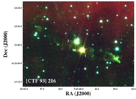
Figure 16: Spitzer/IRAC three-colour image (3.6, 4.5, and 8.0 $\mu$m - blue, red, and green, respectively) of the [CTF93] 216 system, sources # 24 (-1), and # 25 (-2), along with their jets (in green). These images were taken in 2006, before the outburst of source # 25.